

Abstract
Purpose
Quantitative Cone Beam CT (CBCT) imaging is increasing in demand for precise image‐guided radiotherapy because it provides a foundation for advanced image‐guided techniques, including accurate treatment setup, online tumor delineation, and patient dose calculation. However, CBCT is currently limited only to patient setup in the clinic because of the severe issues in its image quality. In this study, we develop a learning‐based approach to improve CBCT's image quality for extended clinical applications.
Materials and methods
An auto‐context model is integrated into a machine learning framework to iteratively generate corrected CBCT (CCBCT) with high‐image quality. The first step is data preprocessing for the built training dataset, in which uninformative image regions are removed, noise is reduced, and CT and CBCT images are aligned. After a CBCT image is divided into a set of patches, the most informative and salient anatomical features are extracted to train random forests. Within each patch, alternating RF is applied to create a CCBCT patch as the output. Moreover, an iterative refinement strategy is exercised to enhance the image quality of CCBCT. Then, all the CCBCT patches are integrated to reconstruct final CCBCT images.
Results
The learning‐based CBCT correction algorithm was evaluated using the leave‐one‐out cross‐validation method applied on a cohort of 12 patients’ brain data and 14 patients’ pelvis data. The mean absolute error (MAE), peak signal‐to‐noise ratio (PSNR), normalized cross‐correlation (NCC) indexes, and spatial nonuniformity (SNU) in the selected regions of interest (ROIs) were used to quantify the proposed algorithm's correction accuracy and generat the following results: mean MAE = 12.81 ± 2.04 and 19.94 ± 5.44 HU, mean PSNR = 40.22 ± 3.70 and 31.31 ± 2.85 dB, mean NCC = 0.98 ± 0.02 and 0.95 ± 0.01, and SNU = 2.07 ± 3.36% and 2.07 ± 3.36% for brain and pelvis data.
Conclusion
Preliminary results demonstrated that the novel learning‐based correction method can significantly improve CBCT image quality. Hence, the proposed algorithm is of great potential in improving CBCT's image quality to support its clinical utility in CBCT‐guided adaptive radiotherapy.
Keywords: adaptive radiotherapy, alternating random forest, CBCT correction, feature selection
Short abstract

1. Introduction
Quantitative Cone Beam CT (CBCT) imaging is on increasing demand for precise image‐guided radiation therapy because it provides a foundation for advanced image‐guided radiotherapy.1 With more precise treatment monitoring from accurate CBCT images, dose delivery errors can be significantly reduced in each fraction and further compensated for in subsequent fractions using adaptive radiation therapy. However, the applications of CBCT in clinical practice of radiotherapy are still limited by its image quality, which is not as good as that of planning CT (or diagnostic CT henceforth).2, 3 One major reason underlying the inferior image quality in CBCT is the distortion caused by severe Compton scatter, such as streaking and cupping artifacts, which adversely affects the visibility and uniformity of soft tissues and degrades the accuracy of dose calculation in treatment planning.4
Recently, many scatter correction techniques have been proposed to improve CBCT image quality and facilitate the use of CBCT in radiation therapy.4, 5, 6, 7, 8, 9, 10, 11 These techniques can be roughly grouped by two types: preprocessing‐based methods12, 13, 14, 15, 16 and postprocessing‐based methods.5, 6, 7, 10, 17, 18, 19, 20, 21, 22, 23, 24, 25, 26, 27 The preprocessing‐based methods suppress scatter during projection data acquisition, of which the anti‐scatter‐grid‐based and air‐gap‐based methods are the two most popular ones.2 The anti‐scatter‐grid‐based methods use grids that are customized for CBCT detectors to remove the scattered photons from the beam in projection data acquisition.9, 28, 29, 30, 31 One major disadvantage of these methods is their limited efficacy in scatter correction. Siewerdsen et al.13 reported that the anti‐scatter‐grid‐based method was effective only in improving the contrast‐to‐noise ratio of low resolution CT images. Another drawback is the increase in x‐ray dose to make up for the loss of primary photons due to grid's attenuation. Kyriakou et al.9 reported that the dose increase can be significant while the scatter is intense. The air‐gap‐based methods are well known in improving the contrast resolution in x‐ray images by reducing scattered radiation incident on the detector.32 These air‐gap‐based methods are advantageous in implementation — no additional hardware or algorithm is required. However, these methods need to increase the distance between the imaged target and the CBCT detectors, which may not be feasible in some clinical situations because of limited space and safety regulations. In addition, due to a large distance between the subject and CBCT detector, the x‐ray power has to escalate to maintain the flux at the detector. Therefore, the efficacy of scatter reduction by preprocessing‐based methods is limited.
The postprocessing‐based methods first estimate the scatter based on prior knowledge or statistical distribution modeling, then remove the estimated scatter from projection data, and finally reconstruct CBCT images from corrected projection data. These methods can be grouped into the following four categories: (a) measurement‐based methods,33, 34, 35 (b) software‐based methods,10, 22, 36, 37, 38, 39, 40, 41, 42, 43, 44 (c) hardware‐based decomposition methods,6, 25, 26 and (d) hybrid methods.39, 40 More details about these postprocessing‐based methods can be found in the review paper by Niu et al.2 These postprocessing‐based methods may either simplify the nonlinear scattering process with deterministic modeling or need multiple scans to recover the projection data contaminated by scatter, which may lengthen the scan time, suffer from involuntary patient motion, and increase patient dose. In addition, these methods share a main disadvantage — the difficulty in suppressing the statistical noise caused by the scatter's high‐frequency components.
In this work, we develop an iteratively refined, anatomical signature‐based, alternating random forest (ARF) method to derive a CCBCT from original CBCT. We aim not only to mitigate the artifacts on CBCT images to the level as that on planning CT images, but also to restore the HU numbers from CBCT to CT images for dose calculation. To the best of our knowledge, the work presented in this paper is the first of such an attempt, which may make contributions to the field in the following aspects: (a) Automatic selection of attributes in features that are the most relevant to the correction modeling using the least absolute shrinkage and selection operator (LASSO) and fuzzy c‐means labeling. (b) Joint information gain (JIG) for selection of splitting function by reducing both CBCT features’ and planning CT targets’ uncertainty. The intuition of JIG is that the binary splitting procedure not only requires putting training data in a leaf node that has similar CT targets, but also restricts the similarity between those data, which thus enhances the inference ability in the leaf. (c) Application of ARF method in the training model by introducing global loss to optimize the threshold of the splitting function while splitting the data from a parent node to child nodes. (d) Application of auto‐context model (ACM) for iteratively refining ARF's performance by incorporating the contextual information of CCBCT image and combining the originally selected CBCT signatures.
The paper is organized as follows. In methods, we first give an overview of the proposed CBCT correction framework, followed by detailed description of the LASSO‐based anatomical feature selection, ARF construction with a JIG, and ACM for ARF iterative refinement. We evaluate the proposed method with state‐of‐the‐art dictionary‐learning‐based (DL) method and verify its performance experimentally using clinical data. Finally, along with an extended discussion, we conclude the presentation of our novel anatomical signature and ACM based ARF CBCT correction method and framework.
2. Materials and methods
2.A. Overview
We first build a training dataset consisting of multiple paired CBCT and CT images. The CT images were acquired using a Siemens SOMATOM Definition AS CT scanner at 120 kVp with the patient in treatment position. The image spacing was 0.586 mm × 0.586 mm × 0.6 mm and 0.98 mm × 0.98 mm × 2.0 mm for brain and pelvis patients, respectively. The CBCT images were acquired using the Varian On‐Board Imager CBCT system at 125 kVp. The image spacing was 1.17 mm × 1.17 mm × 2.5 mm for brain patients and 0.908 mm × 0.908 mm × 2.0 mm for pelvis patients. The CBCT used in this study was acquired from the first fraction of treatment for each patient, which is closest to the planning CT. Given the paired CBCT and planning CT images, the CT image serves as the regression target of CBCT. Before training, image preprocessing, including denoising and suppressing nonuniformity by a nonlocal means method,45 is performed to improve the training's performance. Then, a rigid registration is performed to establish an alignment of subjects between the paired CBCT and CT images, followed by aligning all subjects onto a common space via rigid‐body inter‐subject registration. The inter‐subject registration is performed between two subjects to roughly bring all subjects onto a common space. All the training pairs are further registered to the new CBCT image. In the training phase, given a CBCT image, we initially extract the features at multi‐levels, that is discrete cosine transform (DCT), local binary pattern (LBP), and pair‐wise voxel difference features at multi‐scales, including coarse, medium, and original resolutions. The 3D patch‐based DCT features are extracted to characterize patches in frequency space.46 The 3D patch‐based LBP features are extracted by using rotation invariant LBP extractors.47 The pair‐wise voxel difference features are extracted by computing the intensity difference from a pair of randomly chosen voxels at different locations within 3D patch.48
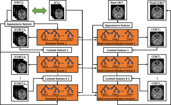
Second, we introduce a logistic LASSO‐based feature selection method for high‐dimensional and nonselective feature sets, and then use it in combination with corresponding CT labels to select the most relevant and informative subset of signatures. Third, the selected informative features with the corresponding CT targets are used to train a sequence of improved random forests (RF) under the framework of ACM. In contrast to the traditional RF, which is usually trained in a depth‐first manner without control over the regressor, a breadth‐first ARF,49 which has a major advantage of checking the state of the training model by measuring its performance against a global loss, is used for training the RF. In order to reduce the ambiguity caused by purely reducing the uncertainty of CT targets in training the model, a JIG considering both CBCT and CT images is introduced for selecting the adaptive splitting function of ARF. In the testing phase, we extract selected anatomical features50 from the new CBCT and then feed into the well‐trained ARF sequence for correction in CBCT image. Figure 1 shows a brief workflow of the proposed method.
Figure 1.
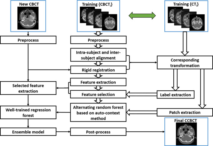
The schematic flow diagram of the proposed method. [Color figure can be viewed at wileyonlinelibrary.com]
2.B. Feature selection
We first introduce the notation to be used in this subsection. denotes the feature set in CBCT image patches centered at each voxel , and denotes the set of corresponding CT central voxels that are regarded as the targets of the training model. In each CBCT image patch, we have an extremely high‐dimensional signature that has presented a serious disadvantage to a learning model. One major problem is that the high‐dimensional signature may contain noisy and redundant information that could overfit the learning models, leading to degraded performance in estimation accuracy and correction.51
Since feature selection can be regarded as a binary regression task about each dimension of the original feature,52, 53 a logistic regression function is used to denote a conditional probability model with the form defined by
| (1) |
where represents the original feature signature of voxel , and is the binary coefficient with 1 indicating that the corresponding features are relevant to the anatomical classification, and 0 denoting that the nonrelevant features are eliminated during the classifier learning process. l(·) is an anatomical binary labeling function. Two‐step feature selection is applied by using l(·) to label air and non‐air materials in first round and then to label bone and soft tissue in the second round. In the paired CBCT‐CT images for training, the fuzzy C‐means clustering method is used to roughly classify the CT image into three segments: air, soft tissue, and bone. Moreover, the goal of feature selection was to pick up a small subset of the most informative features as anatomical signature, which can be accomplished by implementing the sparsity constraint in the logistic regression, that is minimizing the following LASSO energy loss function:
| (2) |
where denotes the sparse coefficient vector, the intercept scalar, the optimization scalar and the regularization parameter, denotes the number of voxel samples and denotes the length of vector . is computed by discriminative power, that is Fisher's score54 for each feature of feature vector. The optimization tries to penalize the features that have smaller discriminative power, that is, uninformative features being eliminated for training the learning‐based model. To implement this penalty, is divided by .
Denoted as , the informative features corresponding to the nonzero entries in are selected, which have superior discriminatory power in distinguishing bone, air, and soft tissue.
An example is given in Fig. 2, in which (a) shows a CBCT image with two types of samples. The samples coming from the bone are indicated by red asterisk while those from the soft tissue by green circles. And (b) shows a scattered plot of the samples corresponding to the randomly selected two features (located in LBP features) without feature selection, while (c) shows that of the samples corresponding to the two top‐ranked features (located in DCT features), which are evaluated by Fisher's score,54 after feature selection.55 It is observed that, with feature selection, the bone is well separated from the soft tissues.
Figure 2.
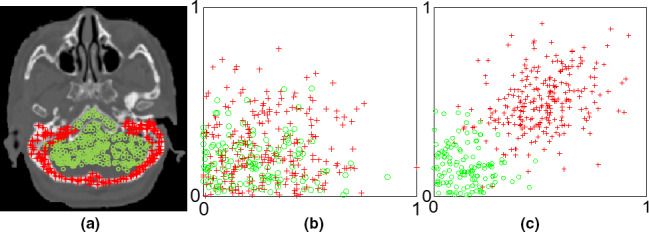
An example illustrates the benefit of feature selection in material separation. [Color figure can be viewed at wileyonlinelibrary.com]
2.C. Alternating regression forest
Recent studies have used the RF to train regression models, due to its efficacy in tackling medical image processing challenges.48, 56 RF trains a bag of decision trees, each of which is provided with a random subset of training data and trained independently. Specifically, in this work, the training data are composed of selected features , as proposed in Section 2.B, and CT targets . Given a subset of training data , the training of decision tree involves recursively splitting a node (denoted by parent node) into two disjoint partitions (denoted by left and right child nodes), such that the uncertainty of CT targets in the resultant subsets is minimized. In particular, the splitting procedure is carried out firstly by randomly choosing ‐th feature and then randomly sampling a set of splitting functions to separate the given data into two disjoint subsets. Corresponding to each feature, each splitting function is a binary decision function parameterized by the feature's position and threshold . The CT target is then separated into and , where denotes the sample set including paired extracted CBCT features and corresponding CT central voxel in the parent node of decision tree. Subsequently, given each splitting function, the information gained in the separating procedure is measured as , where H(·) is entropy over the targets and usually represented by the variance of all target values . denotes the mean value of target voxels’ value in . Then, the splitting function with the highest information gain is fixed for this node and splits the training data accordingly into two subsets and . This procedure continues until some stopping criteria are met, for example the maximum tree depth or a minimum number of training data left in the splitting node. Once the criteria are fulfilled, a leaf node is created by storing the training data at this node. For a new CBCT feature arriving at each leaf node followed by the previous splitting rules, in order to infer its correspondence to the CT target, a median ensemble model generates the final estimation by computing the median of all the nodes within each decision tree, and then computing the median of all the decision trees. The median ensemble can avoid the potential bias, because CBCT images can be roughly grouped in three regions (bone, air, and soft tissue) with significant different intensity values, the use of median can guarantee the prediction result to be either air, bone or soft tissue. Thus, even if there are some positioning difference in pair‐wise CBCT and CT patches, the median prediction can avoid the potential bias.
However, due to intensity and resolution difference between CBCT and CT image structures, the conventional RF‐based CBCT correction may become unstable. The splitting function of growing a decision tree is purely decided according to CT targets while the training data are composed of both CBCT features and CT targets, and thus the uncertainty of CBCT features with more complicated and diverse variation is ignored. A simple example is shown in Fig. 3, in which the red and yellow squares denote the CBCT image patches and their counterparts in the CT image, while the circles denote the center voxels of each image patch. In Fig. 3(b), the two CBCT patches have dissimilar structures that would result in diversity in their extracted features, while in Fig. 3(a) the central voxels of the corresponding CT patches are of similar intensity. If a subset of training data includes these two pairs of CBCT features and CT targets for an internal node, the uncertainty of only CT targets is minimized with different CBCT structures distributed in a uniform partition, regardless of the feature that would be chosen for separation and the splitting function that would be applied for separation. Thus, the splitting procedure with respect to reduction of CT targets’ uncertainty may induce ambiguity to the training of decision tree.
Figure 3.
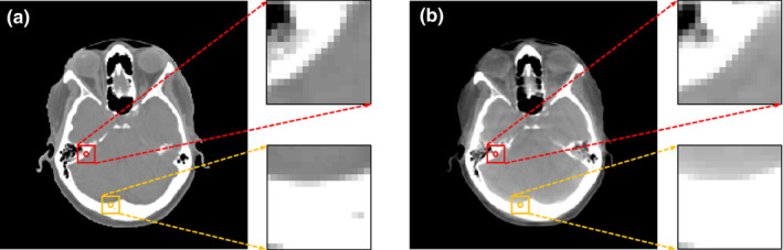
An example of a CT‐CBCT pair. (a) is the CT image and (b) is the corresponding CBCT image. [Color figure can be viewed at wileyonlinelibrary.com]
In training a bag of binary decision trees, the RF for CBCT correction makes a local decision at each node level on how the data are further split by measuring information gain without considering the regressors’ state. Given a subset of training data, the information gain of each splitting function is minimized greedily and independently via reducing the uncertainty of CT targets. Although these characteristics can result in fast and parallel training capabilities and thus higher computational efficiency, the training procedure of RF is not globally controlled by an appropriate metric of the regressors’ performance, and the entire state of training model cannot be promptly checked and improved at each node. This makes the training procedure theoretically difficult and unintuitive to comprehend the success of a learning method.
In practice, there is no guarantee that all thresholds of splitting functions have been learned properly. Moreover, it is difficult to apply the RF in CBCT correction, since the extracted CBCT features are usually in a high‐dimensional representation space and only a small fraction of randomly chosen features could be used for binary splitting. This would compromise the performance of training, thus weaken the inference ability when a new CBCT feature arrives. In order to solve these two issues, we introduce a JIG by combining the information from both CBCT and CT for the splitting function at each node and use an ARF to formulate the training procedure as solving a stage‐wise risk minimization problem for regression tasks, as described in detail below.
- Joint information gain: the conventional RF uses a threshold to split the feature variable to left and right nodes by maximizing the information gain of CT target. As per the definition of information gain, it aims to group the similar CT central voxels to a subset and thus reduces the uncertainty of training data in each child node. However, the CT voxels with similar intensities could be of dissimilar CBCT structural patches, as shown in Fig. 3. The central voxels of the bone near the soft tissue [yellow circle in Fig. 3(b)] and those near the air [red circle in Fig. 3(b)] are similar in intensity, but differ in the structures in CBCT patches, which can become a negatively biased voting of the most adaptive splitting function used for separation and may degrade the performance of regression. Thus, one needs to consider both feature and target into the definition of JIG:
where is a smoothing parameter, denotes the mean over feature vectors, denotes the mean value of target voxels’ value . The first term in Eq. (3) utilizes CT targets’ information, while the second term enforces the similarity in feature space via balancing parameter . The intuition of this regularization is that binary splitting requires both similarity of CT targets and CBCT features. After setting the best splitting function based on Eq. (3), the data of current node are divided into the left and right child nodes. The splitting procedure continues until a preset stopping criteria is met.(3) - Alternating Random Forest: The conventional RF pays no attention to information loss while data are split from parent node to child node. Inspired by the idea of introducing a global loss in recent ARF studies,49 we propose a novel splitting procedure considering both global and local optimization. First, the global loss function can be written as a breadth‐first missing error measured by all weak inference learners at each depth:
where is the training dataset of both CT targets and CBCT features. Loss(·) is a differentiable loss function and denotes the regressor that is already trained from the root node to depth . is collection of the thresholds that are fixed by the last depth of splitting. denotes the regressor at current depth , and θ d is the set of splitting thresholds to be trained at the current depth by minimizing Eq. (4).(4)
Together with our previous study in JIG, the splitting function can be further optimized by maximizing JIG and minimizing the global loss at the current depth:
| (5) |
The first term of Eq. (6) is the JIG specified in Eq. (3), the second term is the global loss regularization specified Eq. (4), while is a parameter to balance the need for regression. At the root node, we start with an initial regressor , with its splitting function being selected by maximizing Eq. (3) and then add a depth regressor that is decided by optimizing the splitting threshold in Eq. (6), to the forest. At each depth, a previous regressor generates the training CBCT targets as by a median ensemble model according to the stored training data at corresponding nodes. These corrections yield a corresponding loss which should be minimized by Eq. (4). After the threshold optimization in Eq. (6), the regressor can be determined at the current depth according to JIG maximizing criterion. Since the splitting function at each node and each depth is chosen by jointly reducing the uncertainty of training data and minimizing the whole regressors’ global loss, unlike the conventional RF whose path of splitting training data is independent beforehand for each node, our proposed ARF allows the splitting path to be optimized globally and locally as we have a hierarchical splitting structure. Thus, the feedback at each depth reasonably reduces the uncertainty of binary decision tree and enhances the accuracy of inference. Figure 4 briefly shows the framework of our proposed learning method, with the default parameters listed in Table 1.
Figure 4.
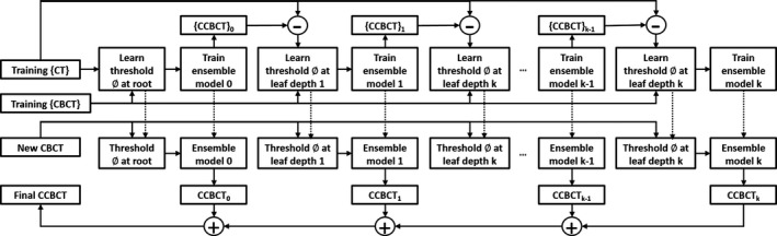
Algorithmic architecture of the alternating regression forest approach.
Table 1.
Default parameter setting
| Parameter | Default value |
|---|---|
| Number of trees | 20 |
| Maximum number of training data in leaf node | 5 |
| Maximum depth of tree | 20 |
| Smoothing parameter λ of information gain (3) | 0.05 |
| Balancing parameter Ƴ used in Eq. (6) | 0.05 |
2.D. Auto‐context model
Since RF is a collection of weak learners, ACM,57, 58 with its framework presented in Fig. 5, is used in the proposed method to enhance its performance by leveraging the surrounding information in regard to the object of interest. We use the initial ARF and feature selection to create contextual features for all training data, which are then utilized in combination with the initial anatomic signature to train an improved ARF. The process is repeated to train a series of ARFs until the criterion of correction accuracy is met. In the testing stage, a new CBCT image can follow the same sequence of ACM to generate the final CCBCT. The proposed method is summarized in Framework 1.
Figure 5.
Algorithmic architecture of auto‐context modeling. [Color figure can be viewed at wileyonlinelibrary.com]
Framework 1. CBCT correction using anatomic signature and auto‐context alternating random forest
|
3. Results
3.A. Datasets and quantitative measurements
In order to test its performance, we applied our method on the planning CT and CBCT data of 12 patients’ brain images and 14 patients’ pelvis images. The leave‐one‐out cross‐validation approach was used in performance evaluation, in which the obtained CCBCT images were compared with their counterparts in planning CT images. The mean absolute error (MAE), peak signal‐to‐noise ratio (PSNR), and normalized cross‐correlation (NCC) indexes were used to quantify the results. MAE, PSNR, and NCC are used to measure the absolute difference, relative difference, and image similarity, which are defined as follows,
| (6) |
| (7) |
| (8) |
where is HU of planning CT, is that of the CCBCT, the maximum intensity of and , and the number of voxels. and are the mean of CT and CCBCT image, while and are the standard division. The unit of MAE is HU and the unit of PSNR is decibel (dB). Spatial nonuniformity (SNU) is also calculated, defined/formulated as Ref. 41, 59.
| (9) |
and are the maximum and the minimum of the mean CT number values of regions of interest (ROIs), respectively. Different ROIs were selected in the CBCT image at both the center and the periphery.
In addition to image quality, we also evaluated the dosimetric accuracy of our results. We applied the original treatment plan on the uncorrected/corrected CBCT images to calculate dose and compared them with that on original planning CT. Clinical relevant dose‐volume histogram (DVH) metrics were selected for comparison.60
3.B. Parameter performance
In general, the performance of correction can be improved with more decision trees and larger maximum depth of each decision tree. However, computation complexity (enlarged by larger number of decision trees and larger maximum depth of decision tree) and algorithm accuracy is a trade‐off in our learning‐based CBCT correction. We first fixed the maximum tree depth and tested the number of trees. Figures 6(a1)–6(a3) visualize the MAE, PSNR and NCC metrics with different number of trees, where other parameters are fixed as the default values in Table 1. It is observed that 24 trees are adequate for our CBCT correction application. In addition to the number of decision trees, the performance of the proposed CBCT correction method also depends on the maximum depth in the decision tree. Figures 6(b1)–6(b3) visualize the performance as assessed in MAE, PSNR and NCC as function of the maximum depth of decision trees, in which other parameters are set at the default values (Table 1). Those plots show that 22 is an adequate maximum tree depth for the proposed CBCT correction method. We set = 0.5 in Eq. (2), = 0.05 in Eq. (3) and = 0.05 in Eq. (6). is a regularization parameter in feature selection; it is used to balance the two terms in LASSO energy loss function. Determining the optimal value for the regularization parameter is an important part of ensuring that the feature selection performs well, and it is typically chosen using cross‐validation.61 We test the parameter from 0.1 to 1.0 by 4‐fold cross‐validation, the performance is stable when = 0.5. is a balancing parameter in computing the information gain, and is designed based on its performance on balancing the information energy of CT target and MR features.62 In fact the MR features’ length is much bigger than CT target, which means the MR features have more information energy than CT target. Thus, should be very small, and we set it to 0.05. is also a balancing parameter to balance the information gain and global loss in optimization of splitting procedure of each decision tree.49 Because the splitting procedure of earlier depth, such as the first splitting procedure from a root node to it child nodes, is mainly affected by information gain. Thus should be small. After several depths of splitting procedure, the information gain is minimized and the global loss has a main effect to converge the training. We found that = 0.05 is good in this study. We also set the maximum number of training data in leaf node to 5 as recommended in the guidance of regression forest.
Figure 6.
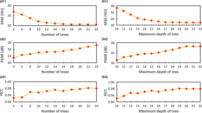
(a1–a3) show the performance of the proposed CBCT correction method assessed by mean absolute error (MAE), peak signal‐to‐noise ratio (PSNR) and normalized cross‐correlation (NCC), as function of the number of decision trees. (b1–b3) show the performance of the proposed CBCT correction method assessed by (a) MAE, (b) PSNR, and (c) NCC, as function of the maximum depth in decision tree. [Color figure can be viewed at wileyonlinelibrary.com]
3.C. Contribution of feature selection
We tested the influence of feature selection on performance of the proposed CBCT correction and the results are presented in Fig. 7, in which the RF method without feature selection is denoted by RF, whereas that with feature selection is denoted by RF + FS. It is observed that RF + FS outperforms RF, since the former reserves the informative anatomical features in the training stage. Table 2 lists results of the leave‐one‐out experiments, which quantitatively reinforces the observation in Fig. 7.
Figure 7.
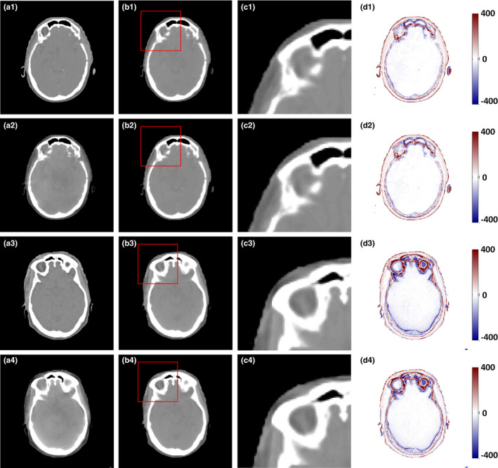
Comparison of the results with and without feature selection. (a1) and (a3) are the planning CT, (a2) and (a4) are the corresponding CBCT images, (b1–d1) and (b3–d3) are the CCBCT images, zoomed regions indicated by red boxes, and difference images between planning CT and CCBCT given by RF; (b2–d2) and (b4–d4) are CCBCT images, zoomed regions indicated by red boxes, difference images between planning CT and CCBCT given by RF + FS. Display windows are [−400, 400] HU for all the subfigures. [Color figure can be viewed at wileyonlinelibrary.com]
Table 2.
Quantitative performance evaluation over the RF‐based CBCT correction method with and without feature selection
| Method | MAE (HU) | PSNR (dB) | NCC |
|---|---|---|---|
| RF | 18.027 ± 3.660 | 38.762 ± 3.387 | 0.984 ± 0.016 |
| RF + FS | 16.777 ± 3.232 | 39.247 ± 3.449 | 0.984 ± 0.016 |
3.D. Contribution of the proposed random forest based on ARF and JIG
We tested our proposed ARF method with the RF + FS method. Fig. 8 provides a detailed visual comparison among RF + FS and RF + FS method with JIG (RF + FS + JIG) and ARF + FS method with JIG (ARF + FS + JIG). The RF + FS + JIG and ARF + FS + JIG methods show better performance than the RF + FS method, since the combined CBCT and CT information and breadth‐first global loss are used in our proposed methods. Figures 8(c1)–8(c6) presents zoomed view of regions adjacent to the bone and soft tissue. Table 3 confirms the above observations quantitatively through the leave‐one‐out experiments. The ARF + FS + JIG‐based method can significantly decrease MAE and improve PSNR compared with RF + FS‐based (P < 0.001 for MAE; P < 0.01 for PSNR) and RF + FS + JIG‐based (P < 0.001 for MAE; P < 0.01 for PSNR) methods.
Figure 8.
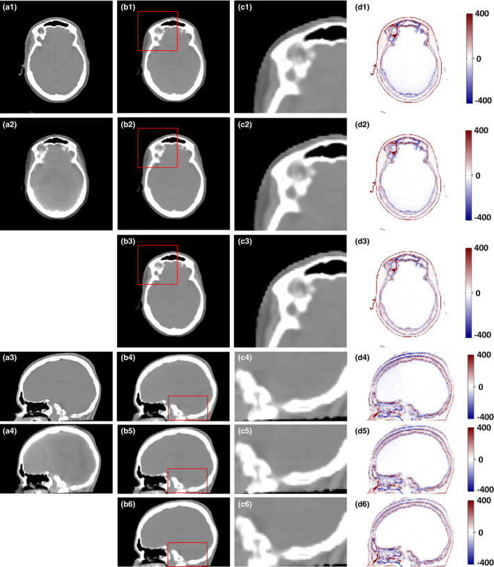
Comparison of the results with different methods. (a1) and (a3) are the planning CT, (a2) and (a4) are the original CBCT images, (b1–d1) and (b4–d4) are the CCBCT images, zoomed regions indicated by red boxes, and difference images between planning CT and CCBCT given by RF + FS; (b2–d2) and (b5–d5) are the CCBCT image, zoomed regions indicated by red boxes, and difference images between planning CT and CCBCT given by RF + FS + JIG; (b3–d3) and (b6–d6) are the CCBCT image, zoomed regions indicated by red boxes, and difference images between planning CT and CCBCT given by ARF + FS + JIG. Display windows are [−400, 400] HU for all the subfigures. [Color figure can be viewed at wileyonlinelibrary.com]
Table 3.
Quantitative performance evaluation over the RF + FS, RF + FS + JIG and ARF + FS + JIG methods
| Method | MAE (HU) | PSNR (dB) | NCC |
|---|---|---|---|
| RF + FS | 16.777 ± 3.232 | 39.247 ± 3.449 | 0.985 ± 0.016 |
| RF + FS + JIG | 15.659 ± 2.834 | 39.526 ± 3.509 | 0.985 ± 0.016 |
| ARF + FS + JIG | 14.744 ± 2.489 | 39.598 ± 3.592 | 0.985 ± 0.016 |
3.E. Contribution of ACM
The improvement of ACM in the proposed method was showed by testing the ARF with four repeating refinement iterations. Along with the iterative enhancement by comparing the structural detail in the sagittal view of CCBCT images in Figs. 9(b1)–9(e1), 9(b2)–9(e2), 10 quantitatively confirms the improvement in the performance over iteration.
Figure 9.
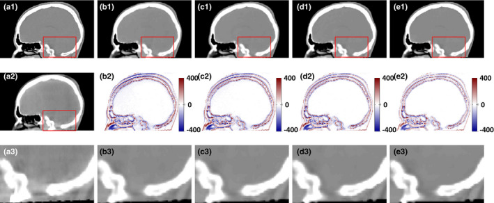
Improvement in the performance over iterations. (a1) planning CT, (a2) CBCT, (b1–e1) CCBCT results corresponding to 1, 2, and 3 iteration of; (a2–e2) corresponding difference images between planning CT and CCBCT (b1–e1). (a3) shows the zoomed regions indicated by red boxes in (a2). (b3–e3) show the zoomed regions indicated by red boxes in (b1–e1). Display windows are [−400, 400] HU for all the subfigures. [Color figure can be viewed at wileyonlinelibrary.com]
Figure 10.
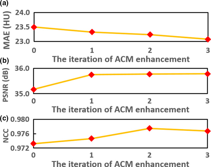
(a) Improvement in the performance as assessed by (a) mean absolute error, (b) PSNR, and (c) normalized cross‐correlation, over iteration of refinement. [Color figure can be viewed at wileyonlinelibrary.com]
3.F. Comparison with conventional scatter correction method
To evaluate the performance, we conducted a study to compare the performance of our proposed method, that is, ARF + FS + JIG combined with ACM (denoted by ARF + ACM + FS + JIG) against a state‐of‐art conventional scatter correction method44 on both pelvic phantom and patient data. The main idea of this scatter correction method is estimating a map of nonuniformity by segmenting images into basic materials. On phantom data, we used odd CBCT image slices and associated CT images to train our learning‐based method and performed the evaluation on even image slices. For each input image, we generated a “duplicate” image that was shifted, zoomed in/out, rotated, and flipped. Figure 11 shows the comparison between these two methods. Compared with conventional scatter correction method, our method shows comparable image quality and better quantitative results on phantom study, and a significant improvement in image quality on patient data. As shown in Figs. 11(a3)–11(a4), both methods can enhance the image quality of CBCT phantom very well. On patient data, our ARF + ACM + FS + JIG can degenerate the beam artifact in CCBCT image much better than the conventional correction method, which can be seen in Fig. 11(b3)–11(b4). The metric comparison is shown in Table 4, where MAE, PSNR, NCC, and SNU computed by selected eight ROIs as shown in solid rectangles in Figs. 11(a1) and 11(b1) are used. Table 4 demonstrates that our ARF + ACM + FS + JIG quantitatively outperforms the conventional scatter correction method.
Figure 11.
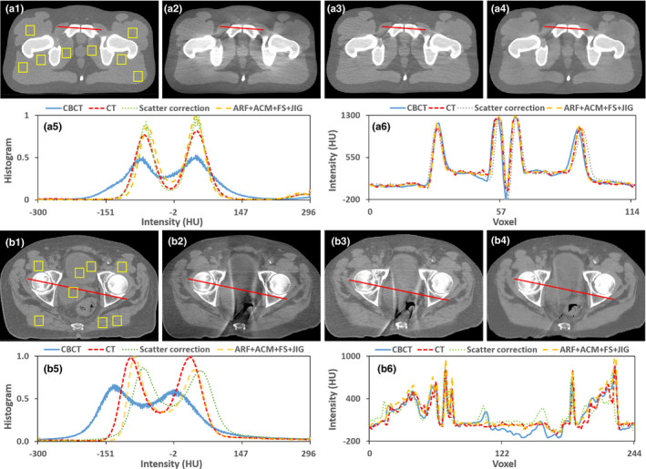
Comparison of the proposed algorithm and a conventional correction method44 with pelvic patient and phantom data. (a1–a6) are the phantom CT, CBCT image without correction, the result obtained by a conventional correction method, the result generated by our ARF + ACM + FS + JIG, the histogram plots in (a1–a4) and the profiles through the red solid line in (a1–a4), respectively. (b1–b6) are the patient planning CT, CBCT image without correction, the result obtained by this conventional correction method, the result generated by our ARF + ACM + FS + JIG, the histogram plots in (b1–b4) and the profiles through the red solid line in (b1–b4), respectively. Display windows are [−400, 400] HU for (a1–a4) and (b1–b4). [Color figure can be viewed at wileyonlinelibrary.com]
Table 4.
Quantitative performance evaluation over the conventional scatter correction method and ARF + ACM + FS + JIG methods on both pelvic phantom and patient data
| Method | Phantom data | Patient data | ||||||
|---|---|---|---|---|---|---|---|---|
| MAE (HU) | PSNR (dB) | NCC | SNU (%) | MAE (HU) | PSNR (dB) | NCC | SNU (%) | |
| Conventional method 44 | 15.526 | 38.340 | 0.969 | 9.120 | 38.576 | 34.736 | 0.938 | 15.774 |
| Our method | 10.228 | 41.886 | 0.989 | 5.001 | 12.324 | 39.768 | 0.973 | 7.561 |
3.G. Comparison with machine learning‐based method
In order to further evaluate and verify the performance, we conducted a study to compare the performance of our proposed ARF + ACM + FS + JIG method against that of state‐of‐art dictionary‐learning (DL)‐based approach.63, 64 The DL‐based method is one of popularly used method to improve CBCT image quality including artifact correction and HU restoration. Both of DL‐based method and our learning‐based method use patch‐based concept, so they are very comparable at this point. The main idea in the DL‐based method is that each local patch of new CBCT can be linearly and sparsely represented by the training CBCT patches. The resultant sparse coefficients are then used to generate new CCBCT patch from corresponding planning CT patches in the training dataset. The results are shown in Fig. 12, in which the CCBCT image generated by ARF + ACM + FS + JIG is quite similar to that of the planning. As can be seen, the DL‐based method results in blurred and erroneous correction. Table 5 shows that ARF + ACM + FS + JIG outperforms the DL‐based method in terms of MAE, PSNR and NCC. ARF + ACM + FS + JIG achieves: an averaged MAE of 12.809 HU, which is significantly better than 20.891 HU obtained by the DL‐based method (P < 0.001); an averaged PSNR of 40.215 dB, better than 38.059 dB obtained by the DL‐based method (P < 0.001); and an averaged NCC of 0.987, better than 0.982 obtained by DL‐based method (P < 0.005). The plots in Fig. 13 show the performance of the proposed CBCT correction method over patients. As reference, the CBCT images without correction (WC) are presented in Fig. 13, as well as the associated quantitative performance indexes in Fig. 12 and Table 5, respectively.
Figure 12.
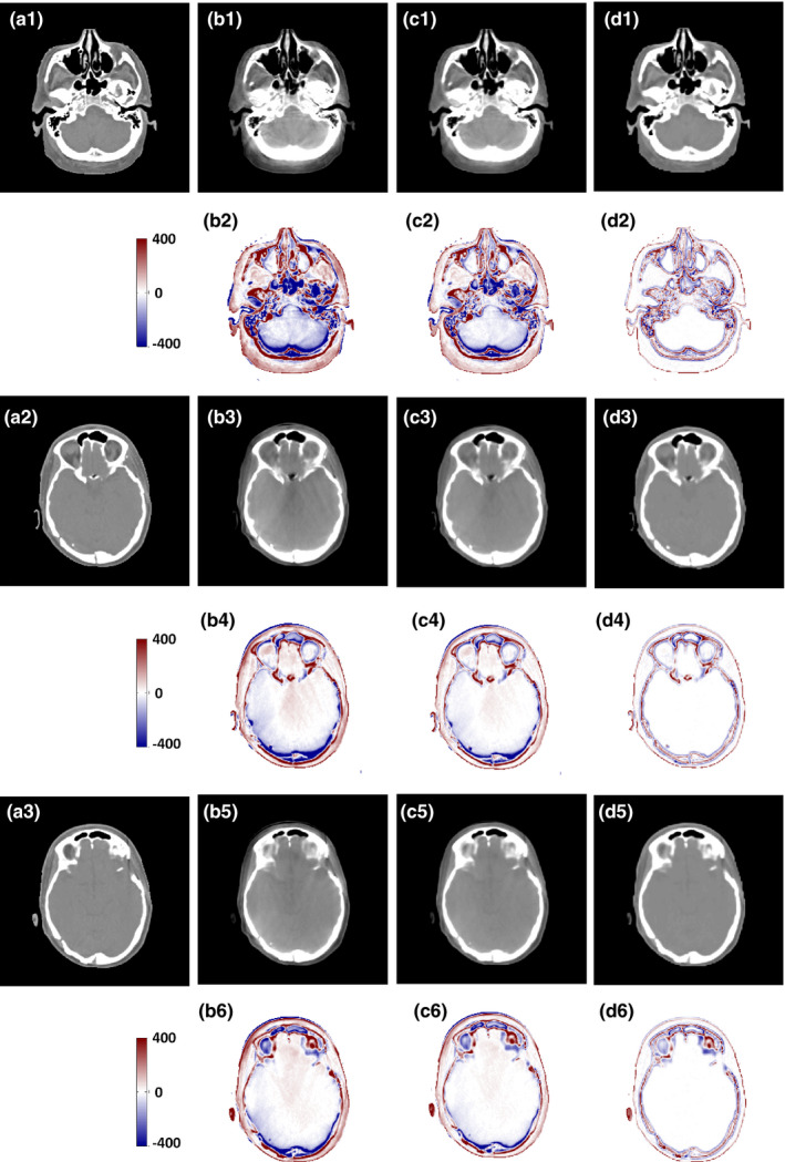
Comparison of the results with the DL‐based method, (a1–a3) are planning CT, (b1), (b3), and (b5) are the CBCT images without correction, (b2), (b4), and (b6) are the difference images between the planning CT and the CBCT without correction; (c1), (c3), and (c5) are the CCBCT results of the DL‐based method, (c2), (c4), and (c6) are the difference images between the CT and the CCBCT results achieved by DL‐based method, (d1) (d3) and (d5) are the CCBCT results of ARF + ACM + FS + JIG, (d2), (d4), and (d6) are the difference images between the planning CT and the CCBCT results obtained by ARF + ACM + FS + JIG. Display windows are [−400, 400] HU for all the subfigures. [Color figure can be viewed at wileyonlinelibrary.com]
Table 5.
Quantitative performance evaluation over the WC, DL and ARF + ACM + FS + JIG methods
| Method | MAE (HU) | PSNR (dB) | NCC |
|---|---|---|---|
| WC | 27.815 ± 6.640 | 35.639 ± 3.265 | 0.976 ± 0.017 |
| DL | 20.891 ± 4.582 | 38.059 ± 3.913 | 0.982 ± 0.016 |
| ARF + ACM + FS + JIG | 12.809 ± 2.041 | 40.215 ± 3.695 | 0.987 ± 0.016 |
Figure 13.
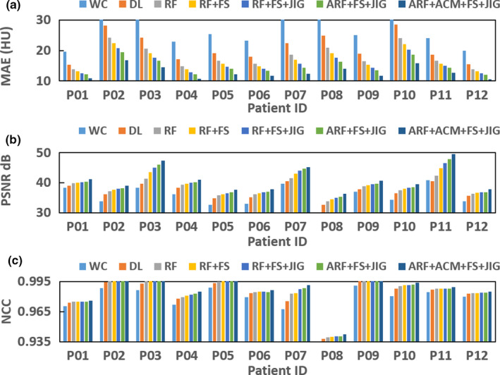
(a–c) show the mean absolute error, peak signal‐to‐noise ratio, normalized cross‐correlation of different methods for each patient's brain data. [Color figure can be viewed at wileyonlinelibrary.com]
3.H. Correction on pelvis and brain data
As the field of view in cranial region is relatively small, scatter contamination is of much less concern as compared to regions of the large field of view, such as pelvic region. Thus, we also included pelvic data in the study, and compared CCBCT with the proposed final algorithm to CBCT without any correction, as shown in Fig. 14. Also, we selected eight ROIs and six ROIs, as shown in solid red rectangles in Figs. 14(a1) and 14(c1), and computed their SNU. The SNU for brain CBCT is 6.959 ± 4.932%, and reduced to 2.070 ± 3.355% with our proposed correction algorithm. The SNU for pelvic CBCT is 27.243 ± 14.088%, and reduced to 15.609 ± 7.766% with correction. The numerical metric comparison on pelvic data is shown in Table 6.
Figure 14.
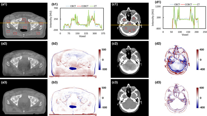
Evaluation of proposed algorithm with pelvic and cranial data, (a1) and (c1) are the planning CT, (a2) and (c2) are the CBCT images without correction, (b2) and (d2) are the difference images between the planning CT and the CBCT without correction; (a3) and (c3) are the CCBCT results of our ARF + ACM + FS + JIG, (b3) and (d3) are the difference images between the planning CT and the CCBCT results obtained by our ARF + ACM + FS + JIG. (b1) and (d1) are the histogram plot of orange solid line in (a1) and (c1). Display windows are [−500, 500] HU for (a1–a3) and (b2–b3), and [−400, 400] HU for (c1–c3) and (d2–d3). [Color figure can be viewed at wileyonlinelibrary.com]
Table 6.
Quantitative performance evaluation over the WC and ARF + ACM + FS + JIG methods on pelvic data
| Method | MAE (HU) | PSNR (dB) | NCC | SNU (%) |
|---|---|---|---|---|
| WC | 45.466 ± 12.265 | 26.706 ± 2.885 | 0.942 ± 0.010 | 27.243 ± 14.088 |
| ARF + ACM + FS + JIG | 19.937 ± 5.441 | 31.311 ± 2.846 | 0.952 ± 0.008 | 15.609 ± 7.766 |
Dose differences using the CBCT occur mostly around streaking artifacts, which are largely mitigated in the CCBCT. The corresponding DVH curves of PTVs and relevant organs at risk (OARs) shown in Fig. 15 indicate that the dose differences in target and avoidance structures are minimal. For pelvic radiotherapy plans, the mean dose error for PTV, bladder, and rectum are significantly reduced, from around 1.0% to 0.3% by our CCBCT.
Figure 15.
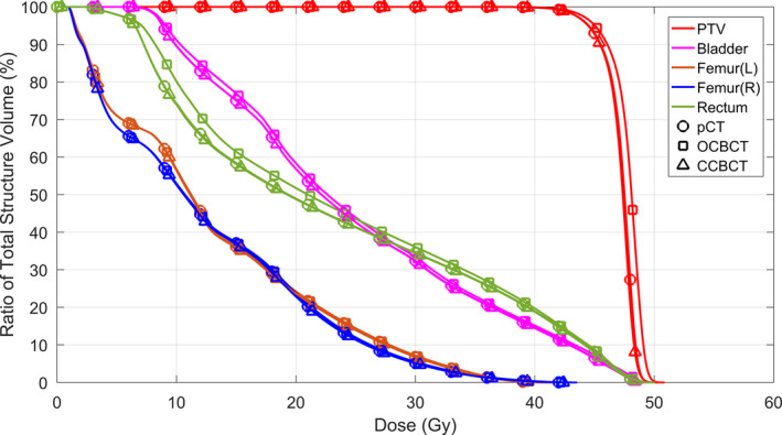
The DVH curves of PTVs and related OARs for pelvic case. OARs for pelvis are bladder, rectum, left femur [Femur(L)], and right femur [Femur(R)]. [Color figure can be viewed at wileyonlinelibrary.com]
4. Discussions
We have proposed a new CBCT correction method that integrates an ACM into a machine learning framework to iteratively improve the image quality of CBCT. An anatomical feature selection and ARF framework were used for CBCT artifact correction. Several mechanisms were incorporated to boost the performance such as ACM and JIG. Our proposed method was evaluated using cranial and pelvic datasets and compared with the performance of advanced DL‐based approach. In summary, this proposed ARF regression with patch‐based anatomical signatures and ACM tries to effectively capture the relationship between CBCT features and target CT. When features of new CBCT are fed into well‐trained RF, corrected CBCT images can be generated with similar image quality (HU intensity) as CT images. The high quality CBCT images can be used to perform quantitative analysis including accurate treatment setup, online tumor delineation, and patient dose calculation.
High‐dimensional signatures contain noisy and redundant features that would overfit the learning models, which may adversely affect the estimation accuracy and degenerate the correction performance. By preselecting the informative anatomical signatures corresponding to segmented labels, the final CBCT correction becomes more accurate. The averaged MAE is 16.777 HU in RF + FS, which is lower than that of RF (averaged MAE = 18.027 HU). The efficacy of feature selection was demonstrated in Fig. 7 and Table 2, showing that the feature selection performed well in correction visually and quantitatively. The proposed JIG remarkably improves the image quality of CCBCT because the binary splitting process in RF using this JIG includes both similarity of CBCT samples and CT targets. The efficacy of using this JIG was demonstrated through Figs. 9(b2)–9(d2), 9(b5)–9(d5) and Table 3, in which the MAE of RF + FS + JIG is 15.659 HU, which was better than that of the RF + FS method. The proposed ARF with the splitting threshold optimization specified in Eq. (6) notably enhances the performance of RF by maximizing JIG and minimizing the introduced global loss simultaneously. The efficiency of ARF + FS + JIG was demonstrated in Figs. 8(b3)–8(d3), 8(b6)–8 (d6) and Table 3. The correction is significantly improved in comparison with the RF+FS method, since ACM iteratively improves the ability of inference in ARF by the contextual information and the original selected signature, as demonstrated in Fig. 9(b)–9(e) and Fig. 10.
With the introduction of the discriminative feature selection, the JIG combining both CBCT and planning CT information, the ARF not only considering the global loss of whole training model but also reducing the uncertainty of training data falling into the child nodes, and the iterative refinement strategy, the proposed method is significantly better than advanced DL‐based method. As shown in Fig. 12, our method can reduce the artifacts and recover true HU in CBCT images, thus significantly improve the image quality of CBCT to a level approaching that of planning CT images, as shown in Table 5 and Fig. 13. In comparison with conventional scatter correction method, as shown in Table 4 and Fig. 11, our proposed method can reduce the artifacts on CBCT images to a similar level as that on planning CT images.
However, although the proposed join information gain and ARF can enhance the performance, the optimization of proposed binary splitting procedure is more complex than traditional binary splitting, and takes more computation time. In addition, we tested our algorithm on 12 patients’ brain data and 14 patients’ pelvis data, in the future we will need to enroll more patients to further evaluate the robustness of our algorithm.
5. Conclusions
In this paper, we proposed an ARF‐based method that integrates anatomical feature selection and ACM to improve CBCT image quality. In the training stage, at multi‐level with multi‐scale sensitivity features derived from each CBCT image, we first extract image information about the local texture, edges, and spatial features. Second, the corresponding CT labels are obtained automatically using fuzzy C‐means labeling. Together with the features and CT labels, we select the most relevant features for modeling of correction by the LASSO operator. The selected features and the corresponding CT targets are used to train a sequence of improved ARFs under the framework of ACM that incorporates the original selected anatomical signatures with the contextual information of the previous CCBCT to train ARFs. In order to reduce the ambiguity caused by the uncertainty in CT targets in model training, a JIG considering both CBCT and CT images is introduced for selecting the adaptive splitting function in ARF. In the testing stage, the selected anatomical features are extracted from new CBCT image and then fed into the well‐trained sequence of ARFs for performing CCBT correction. Experimental results have shown that our method can accurately obtain a CCBCT with high image quality and outperform the advanced DL‐based methods. The proposed method is of great potential in improving CBCT image quality to a level approaching that of planning CT image quality and allowing its quantitative use in CBCT‐guided adaptive radiotherapy.
Conflict of Interest
The authors have no conflicts to disclose.
Acknowledgments
This research is supported in part by the National Cancer Institute of the National Institutes of Health under Award Number R01CA215718 and the Department of Defense (DoD) Prostate Cancer Research Program (PCRP) Award W81XWH‐13‐1‐0269. The authors would like to extend their appreciation to Leonardo Tang for his proofreading of this manuscript.
References
- 1. Xing L, Thorndyke B, Schreibmann E, et al. Overview of image‐guided radiation therapy. Med Dosim. 2006;31:91–112. [DOI] [PubMed] [Google Scholar]
- 2. Niu TY, Zhu L. Overview of x‐ray scatter in cone‐beam computed tomography and its correction methods. Curr Med Imaging Rev. 2010;6:82–89. [Google Scholar]
- 3. Zhu L, Xie YQ, Wang J, Xing L. Scatter correction for cone‐beam CT in radiation therapy. Med Phys. 2009;36:2258–2268. [DOI] [PMC free article] [PubMed] [Google Scholar]
- 4. Xing L, Wang J, Zhu L. Noise suppression in scatter correction for cone‐beam CT. Med Phys. 2009;36:741–752. [DOI] [PMC free article] [PubMed] [Google Scholar]
- 5. Siewerdsen JH, Daly MJ, Bakhtiar B, et al. A simple, direct method for x‐ray scatter estimation and correction in digital radiography and cone‐beam CT. Med Phys. 2006;33:187–197. [DOI] [PubMed] [Google Scholar]
- 6. Zhu L, Bennett NR, Fahrig R. Scatter correction method for x‐ray CT using primary modulation: theory and preliminary results. IEEE T Med Imaging. 2006;25:1573–1587. [DOI] [PubMed] [Google Scholar]
- 7. Ning R, Tang XY, Conover D. X‐ray scatter correction algorithm for cone beam CT imaging. Med Phys. 2004;31:1195–1202. [DOI] [PubMed] [Google Scholar]
- 8. Rinkel J, Gerfault L, Esteve F, Dinten JM. A new method for x‐ray scatter correction: first assessment on a cone‐beam CT experimental setup. Phys Med Biol. 2007;52:4633–4652. [DOI] [PubMed] [Google Scholar]
- 9. Kyriakou Y, Kalender W. Efficiency of antiscatter grids for flat‐detector CT. Phys Med Biol. 2007;52:6275–6293. [DOI] [PubMed] [Google Scholar]
- 10. Kyriakou Y, Riedel T, Kalender WA. Combining deterministic and Monte Carlo calculations for fast estimation of scatter intensities in CT. Phys Med Biol. 2006;51:4567–4586. [DOI] [PubMed] [Google Scholar]
- 11. Niu TY, Sun MS, Star‐Lack J, Gao HW, Fan QY, Zhu L. Shading correction for on‐board cone‐beam CT in radiation therapy using planning MDCT images. Med Phys. 2010;37:5395–5406. [DOI] [PubMed] [Google Scholar]
- 12. Shen SZ, Bloomquist AK, Mawdsley GE, Yaffe MJ, Elbakri I. Effect of scatter and an antiscatter grid on the performance of a slot‐scanning digital mammography system. Med Phys. 2006;33:1108–1115. [DOI] [PubMed] [Google Scholar]
- 13. Siewerdsen JH, Moseley DJ, Bakhtiar B, Richard S, Jaffray DA. The influence of antiscatter grids on soft‐tissue detectability in cone‐beam computed tomography with flat‐panel detectors. Med Phys. 2004;31:3506–3520. [DOI] [PubMed] [Google Scholar]
- 14. Schmidt TG, Fahrig R, Pelc NJ, Solomon EG. An inverse‐geometry volumetric CT system with a large‐area scanned source: a feasibility study. Med Phys. 2004;31:2623–2627. [DOI] [PubMed] [Google Scholar]
- 15. Krol A, Bassano DA, Chamberlain CC, Prasad SC. Scatter reduction in mammography with air gap. Med Phys. 1996;23:1263–1270. [DOI] [PubMed] [Google Scholar]
- 16. Neitzel U. Grids or air gaps for scatter reduction in digital radiography: a model calculation. Med Phys. 1992;19:475–481. [DOI] [PubMed] [Google Scholar]
- 17. Wagner FC, Macovski A, Nishimura DG. Dual‐energy X‐ray projection imaging: two sampling schemes for the correction of scattered radiation. Med Phys. 1988;15:732–748. [DOI] [PubMed] [Google Scholar]
- 18. Yaffe MJ, Johns PC. Scattered radiation in diagnostic‐radiology ‐ magnitudes, effects, and methods of reduction. J Appl Photogr Eng. 1983;9:184–195. [Google Scholar]
- 19. Boone JM, Seibert JA. An analytical model of the scattered radiation distribution in diagnostic‐radiology. Med Phys. 1988;15:721–725. [DOI] [PubMed] [Google Scholar]
- 20. Seibert JA, Boone JM. X‐ray scatter removal by deconvolution. Med Phys. 1988;15:567–575. [DOI] [PubMed] [Google Scholar]
- 21. Zellerhoff M, Scholz B, Ruhrnschopf EP, Brunner T. Low contrast 3D‐reconstruction from C‐arm data. Med Imaging 2005. 2005;5745:646–655. [Google Scholar]
- 22. Li H, Mohan R, Zhu XR. Scatter kernel estimation with an edge‐spread function method for cone‐beam computed tomography imaging. Phys Med Biol. 2008;53:6729–6748. [DOI] [PubMed] [Google Scholar]
- 23. Colijn AP, Beekman FJ. Accelerated simulation of cone beam x‐ray scatter projections. IEEE Trans Med Imaging. 2004;23:584–590. [DOI] [PubMed] [Google Scholar]
- 24. Hansen VN, Swindell W, Evans PM. Extraction of primary signal from EPIDs using only forward convolution. Med Phys. 1997;24:1477–1484. [DOI] [PubMed] [Google Scholar]
- 25. Close RA, Shah KC, Whiting JS. Regularization method for scatter‐glare correction in fluoroscopic images. Med Phys. 1999;26:1794–1801. [DOI] [PubMed] [Google Scholar]
- 26. Bani‐Hashemi A, Blanz E, Maltz J, Hristov D, Svatos M. Cone beam x‐ray scatter removal via image frequency modulation and filtering. Med Phys. 2005;32:2093. [DOI] [PubMed] [Google Scholar]
- 27. Love LA, Kruger RA. Scatter estimation for a digital radiographic system using convolution filtering. Med Phys. 1987;14:178–185. [DOI] [PubMed] [Google Scholar]
- 28. Schafer S, Stayman JW, Zbijewski W, Schmidgunst C, Kleinszig G, Siewerdsen JH. Antiscatter grids in mobile C‐arm cone‐beam CT: effect on image quality and dose. Med Phys. 2012;39:153–159. [DOI] [PMC free article] [PubMed] [Google Scholar]
- 29. Sisniega A, Zbijewski W, Badal A, et al. Monte Carlo study of the effects of system geometry and antiscatter grids on cone‐beam CT scatter distributions. Med Phys. 2013;40:051915. [DOI] [PMC free article] [PubMed] [Google Scholar]
- 30. Stankovic U, van Herk M, Ploeger LS, Sonke JJ. Improved image quality of cone beam CT scans for radiotherapy image guidance using fiber‐interspaced antiscatter grid. Med Phys. 2014;41:061910. [DOI] [PubMed] [Google Scholar]
- 31. Usui K, Inoue T, Kurokawa C, Sugimoto S, Sasai K, Ogawa K. Monte Carlo study on a cone‐beam computed tomography using a cross‐type carbon fiber antiscatter grid. Med Phys. 2016;43:3422. [Google Scholar]
- 32. Daartz J, Engelsman M, Paganetti H, Bussiere MR. Field size dependence of the output factor in passively scattered proton therapy: influence of range, modulation, air gap, and machine settings. Med Phys. 2009;36:3205–3210. [DOI] [PubMed] [Google Scholar]
- 33. Maltz JS, Gangadharan B, Vidal M, et al. Focused beam‐stop array for the measurement of scatter in megavoltage portal and cone beam CT imaging. Med Phys. 2008;35:2452–2462. [DOI] [PubMed] [Google Scholar]
- 34. Yan H, Mou XQ, Tang SJ, Xu QO, Zankl M. Projection correlation based view interpolation for cone beam CT: primary fluence restoration in scatter measurement with a moving beam stop array. Phys Med Biol. 2010;55:6353–6375. [DOI] [PubMed] [Google Scholar]
- 35. Huang KD, Shi WL, Wang XY, et al. Scatter measurement and correction method for cone‐beam CT based on single grating scan. Opt Eng. 2017;56:064106. [Google Scholar]
- 36. Mettivier G, Russo P, Lanconelli N, Lo Meo S. Evaluation of Scattering in cone‐beam breast computed tomography: a Monte Carlo and experimental phantom study. IEEE Trans Nucl Sci. 2010;57:2510–2517. [Google Scholar]
- 37. Poludniowski G, Evans PM, Hansen VN, Webb S. An efficient Monte Carlo‐based algorithm for scatter correction in keV cone‐beam CT. Phys Med Biol. 2009;54:3847–3864. [DOI] [PubMed] [Google Scholar]
- 38. Sisniega A, Abella M, Lage E, Desco M, Vaquero JJ. Automatic Monte‐Carlo based scatter correction for x‐ray cone‐beam ct using general purpose graphic processing units (GP‐GPU): a feasibility study. In: IEEE Nuclear Science Symposium and Medical Imaging Conference (Nss/Mic): 3705‐3709; 2011.
- 39. Watson P, Mainegra‐Hing E, Soisson E, El Naqa I, Seuntjens J. Implementation of a fast Monte Carlo scatter correction for cone‐beam computed tomography. Med Phys. 2012;39(6):3625–3625. [DOI] [PubMed] [Google Scholar]
- 40. Thing RS, Bernchou U, Mainegra‐Hing E, Brink C. Patient‐specific scatter correction in clinical cone beam computed tomography imaging made possible by the combination of Monte Carlo simulations and a ray tracing algorithm. Acta Oncol. 2013;52:1477–1483. [DOI] [PubMed] [Google Scholar]
- 41. Xu Y, Bai T, Yan H, et al. A practical cone‐beam CT scatter correction method with optimized Monte Carlo simulations for image‐guided radiation therapy. Phys Med Biol. 2015;60:3567–3587. [DOI] [PMC free article] [PubMed] [Google Scholar]
- 42. Min J, Pua R, Kim I, Han B, Cho S. Analytic image reconstruction from partial data for a single‐scan cone‐beam CT with scatter correction. Med Phys. 2015;42:6625–6640. [DOI] [PubMed] [Google Scholar]
- 43. Liu J, Bourland J. An analytical model for fast computation of scatter estimation in KV cone‐beam CT images. Med Phys. 2013;40:125–125. [Google Scholar]
- 44. Wang TH, Zhu L. Image‐domain non‐uniformity correction for cone‐beam CT. In: IEEE International Symposium on Biomedical Imaging (ISBI); 2017:680‐683.
- 45. Zhang H, Zeng D, Zhang H, Wang J, Liang Z, Ma J. Applications of nonlocal means algorithm in low‐dose x‐ray CT image processing and reconstruction: a review. Med Phys. 2017;44:1168–1185. [DOI] [PMC free article] [PubMed] [Google Scholar]
- 46. Senapati RK, Prasad PMK, Swain G, Shankar TN. Volumetric medical image compression using 3D listless embedded block partitioning. SpringerPlus. 2016;5:2100. [DOI] [PMC free article] [PubMed] [Google Scholar]
- 47. Guo Z, Zhang L, Zhang D. Rotation invariant texture classification using LBP variance (LBPV) with global matching. Patt Recogn. 2010;43:706–719. [Google Scholar]
- 48. Huynh T, Gao YZ, Kang JY, et al. Estimating CT image from MRI data using structured random forest and auto‐context model. IEEE Trans Med Imaging. 2016;35:174–183. [DOI] [PMC free article] [PubMed] [Google Scholar]
- 49. Schulter S, Leistner C, Wohlhart P, Roth PM, Bischof H. Alternating regression forests for object detection and pose estimation. In: IEEE International Conference on Computer Vision; 2013. 10.1109/iccv.2013.59:417-424 [DOI]
- 50. Lei Y, Shu H‐K, Tian S, et al. Magnetic resonance imaging‐based pseudo computed tomography using anatomic signature and joint dictionary learning. J Med Imaging. 2018;5:034001. [DOI] [PMC free article] [PubMed] [Google Scholar]
- 51. Menard S. Logistic Regression: From Introductory to Advanced Concepts and Applications. Thousand Oaks, CA: SAGE Publications; 2010. [Google Scholar]
- 52. Aseervatham S, Antoniadis A, Gaussier E, Burlet M, Denneulin Y. A sparse version of the ridge logistic regression for large‐scale text categorization. Patt Recogn Lett. 2011;32:101–106. [Google Scholar]
- 53. Avalos M, Pouyes H, Grandvalet Y, Orriols L, Lagarde E. Sparse conditional logistic regression for analyzing large‐scale matched data from epidemiological studies: a simple algorithm. BMC Bioinform. 2015;16:S1. [DOI] [PMC free article] [PubMed] [Google Scholar]
- 54. Widyaningsih P, Saputro DRS, Putri AN. Fisher scoring method for parameter estimation of geographically weighted ordinal logistic regression (GWOLR) model. J Phys Conf Ser. 2017;855:012060. [Google Scholar]
- 55. Ayech MW, Ziou D. Automated feature weighting and random pixel sampling in k‐means clustering for Terahertz image segmentation. In: IEEE Computer Society Conference; 2015. 10.1109/CVPRW.2015.7301294 [DOI]
- 56. Andreasen D, Edmund JM, Zografos V, Menze BH, Van Leemput K. Computed tomography synthesis from magnetic resonance images in the pelvis using multiple random forests and auto‐context features. Proc SPIE. 2016;9784:978417. [Google Scholar]
- 57. Tu ZW, Bai XA. Auto‐context and its application to high‐level vision tasks and 3D brain image segmentation. IEEE Trans Patt Anal Mach Intell. 2010;32:1744–1757. [DOI] [PubMed] [Google Scholar]
- 58. Tu ZW. Auto‐context and its application to high‐level vision tasks. IEEE Conf Comput Vis Patt Recogn. 2008;1:735–742. [Google Scholar]
- 59. Fan QY, Lu B, Park JC, et al. Image‐domain shading correction for cone‐beam CT without prior patient information. J Appl Clin Med Phys. 2015;16:65–75. [DOI] [PMC free article] [PubMed] [Google Scholar]
- 60. Wang T, Manohar N, Lei Y, et al. MRI‐based treatment planning for brain stereotactic radiosurgery: dosimetric validation of a learning‐based pseudo‐CT generation method. Med Dosim. 2018; [Epub ahead of print]. 10.1016/j.meddos.2018.06.008 [DOI] [PMC free article] [PubMed] [Google Scholar]
- 61. Lei Y, Tang XY, Higgins K, et al. Improving image quality of cone‐beam ct using alternating regression forest. Proc SPIE. 2018;10573:1057345. [DOI] [PMC free article] [PubMed] [Google Scholar]
- 62. Yang X, Lei Y, Higgins KA, et al. A leaning‐based method to improve cone beam ct image quality for adaptive radiation therapy. Int J Radiat Oncol Biol Phys. 2017;99:S224. [Google Scholar]
- 63. Andreasen D, Van Leemput K, Hansen RH, Andersen JAL, Edmund JM. Patch‐based generation of a pseudo CT from conventional MRI sequences for MRI‐only radiotherapy of the brain. Med Phys. 2015;42(4):1596–1605. [DOI] [PubMed] [Google Scholar]
- 64. Torrado‐Carvajal A, Herraiz JL, Alcain E, et al. Fast patch‐based pseudo‐CT synthesis from T1‐weighted MR images for PET/MR attenuation correction in brain studies. J Nucl Med. 2016;57:136–143. [DOI] [PubMed] [Google Scholar]