Abstract
Background
As a consequence of global warming, heat waves are expected to become more frequent, more intense, and longer. The elderly and persons with chronic diseases are especially vulnerable to health problems due to heat. This article is devoted to the question of the extent to which the effects of heat waves in Germany are changing over time, and whether preventive health measures are working.
Methods
We use a statistical model to quantify the effect of high mean temperatures on mortality. Within this model, different exposure-response curves for the three temporal intervals 1992–2000, 2001–2010, and 2011–2017 are estimated. Attention is also paid to the delayed effect on mortality of high mean temperatures in the preceding week.
Results
Our analysis reveals a clear, systematic association of the mean temperature in the current week, as well as the mean temperature in the preceding week, with weekly mortality. This association is more pronounced for higher age groups and decreases over the years under analysis, with the exception of a relatively weak effect of heat in southern Germany in 1992–2000. The strongest effects were related to the heat waves in 1994 and 2003, with approximately 10 200 and 9600 fatalities, respectively. Approximately 7800 fatalities were estimated for the summer of 2006, and 4700 and 5200 for 2010 and 2015, respectively.
Conclusion
In Germany, as elsewhere, climate change has been causing more frequent, more intense, and longer periods of heat in the summer. The harmful effect of heat on health is reduced by adaptive processes, presumably including successful preventive measures. Such measures should be extended in the future, and perhaps complemented by other measures in order to further diminish the effect of heat on mortality.
Numerous studies have identified heatwaves as a significant risk factor for human health (1– 5). The elderly and those who are already ill are especially severely affected (6, 7). A higher than average number of heatwaves have occurred in Europe in the period since 2000 (8). Anthropogenic climate change has been identified as contributing to several of the major heatwaves in recent years (9– 11). More frequent, more intensive, and longer-lasting heatwaves are anticipated in Central Europe due to the effects of climate change (12– 15).
Climate change also constitutes a major challenge for public health services (16– 18). It affects health directly via extreme weather events, such as heatwaves, but also indirectly, e.g., through altered conditions for vector-transmitted diseases (19– 21).
Long-term exposure to high temperatures can lead to heat-related illness (22). However, deaths related to heat are rarely ascribed to heat exposure; rather, death is usually recorded as occurring due to pre-existing severe illness(es) linked to age-related degeneration, e.g., cardiovascular disease (23). Against this backdrop, statistical procedures have to be used to estimate the number of deaths that occur due to a heatwave.
Various authors used statistical models to help verify the systematic connection between mean weekly temperature and mortality (24– 28). The non-linear influence of temperature on the mortality rate can be quantified with the aid of an exposure–response curve. The aim of our study was to estimate the number of heat-related deaths on the basis of weekly data, taking into account both immediate and delayed effects of high temperatures on mortality. Moreover, we sought to determine whether the impact of heatwaves in Germany has changed over time.
Method
Data
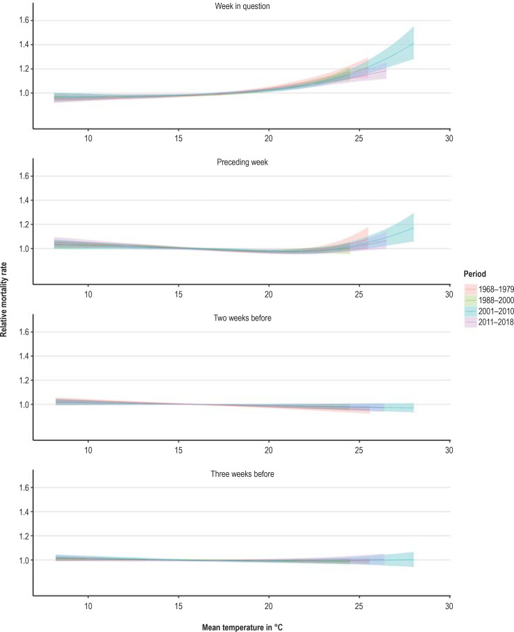
Epidemiological data: We used weekly aggregated data from the Federal Statistical Office on overall mortality in the period 1992 to 2017. The data were aggregated by age group (<65 years, 65–74, 75–84, ≥ 85) and by federal state. Germany was divided into three regions: “northern” (comprising the states Bremen, Hamburg, Mecklenburg–Western Pomerania, Lower Saxony, and Schleswig-Holstein), “central” (Berlin, Brandenburg, North Rhine–Westphalia, Rheinland–Palatinate, Saarland, Hesse, Saxony, Saxony–Anhalt, and Thuringia), and “southern” (Baden–Württemberg and Bavaria). To take account of longer time series, we analyzed data from Baden–Württemberg for the period 1968 to 2018 (eFigure 1a + eFigure 1b).
eFigure 1a.
Course of relative mortality rate (exposure–response curves) in Baden–Württemberg depending on mean temperature in current and foregoing weeks by region in the age group ≥ 85 years. Data: Deaths between the 15th and 40th calendar weeks of the years 1968 to 1979 and 1988 to 2017
Analysis of an extended time series of mortality for Baden–Württemberg
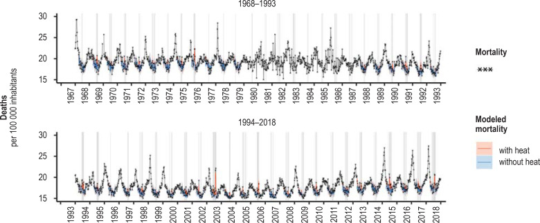
The Statistical Office of Baden-Württemberg has recorded the exact day of decease for all deaths in Baden–Württemberg since 1968. However, analysis of this time series revealed the presence of artifacts for the period 1980 to 1987, so the data from these years had to be removed. Extension of our model to the northern, central, and southern regions of Germany for this longer time series confirms the special role of the years 2001 to 2010, with the heatwave of 2003 constituting a high point for Baden–Württemberg. The foregoing periods show a similar exposure–response curve but without such high mean weekly temperatures. The exposure–response curve is somewhat lower for the period 2011 to 2018—as in the southern region as a whole.
eFigure 1b.
Adaptation of the statistical model to the data on weekly mortality, Baden–Württemberg, 1968–2018. The years 1980 to 1987 were not included in the modeling due to irregularities in the data. Shading shows weeks with a mean temperature of more than 20 °C. Only the weeks in the summer half-year (calendar weeks 15 to 40) were modeled.
Population data: We used the official population statistics of the Federal Statistical Office by federal state and age group for the period 1992 to 2017.
Weather data: The weather data we used were obtained from the ground-level monitoring system of the Deutscher Wetterdienst (Germany’s National Meteorological Service, DWD). For each federal state we selected four to six weather stations located in the main population centers; the sole exception was Mecklenburg–Western Pomerania, where two weather stations were used (Schwerin and Waren [Müritz]).
Modeling
The model describes the time series of observed weekly mortality (number of deaths per number of inhabitants in the target age group) over time, with the aid of three essential components:
An annually recurring seasonal figure that describes the course of mortality through the different times of year
A term for the long-term trend that describes, for example, the increase in life expectancy
The exposure–response curve, which quantifies the effect of heatwaves on mortality
We used the weekly mean temperature as indicator for heat. An der Heiden et al. (1) showed that the weekly mean temperature reflects the observed course of mortality better than the weekly minimum or maximum temperature, the minimum temperature during the warmest night of the week, or comparable measures of humidity or the humidex.
Within the model, all components were estimated separately for the different age groups. To stabilize the model, the model parameter that determined the extent of the random errors was estimated uniformly for the different age groups.
To analyze how the exposure–response curve changed over time, we determined an exposure–response curve for each of the three time segments 1992–2000, 2001–2010, and 2011–2017. To aid comprehension of the influence of dividing the study period in this way, sensitivity analyses were used to evaluate other divisions of the whole period (1992–2017) (etable 1).
eTable 1. Estimated number of heat-related deaths in Germany, 1992–2017 [95% confidence interval]*.
| Year | Primary model, segments: 1992–2000, 2001–2010, 2011–2017 | Alternative model, segments: 1992–2001, 2002–2009, 2010–2017 | Model with short segments: 1992–1997, 1998–2003, 2004–2008, 2009–2013, 2014–2017 | Model with uniform exposure–response curve (1992–2017) | Model with segments as in primary model, but more flexible trend |
| 1992 | 2800 [700; 5000] | 2600 [300; 4900] | 2800 [500; 4700] | 2400 [300; 4800] | 2500 [200; 4700] |
| 1993 | 0 [–2100; 2100] | 100 [–1800; 2200] | 0 [–2200; 1900] | –0 [–1700; 2200] | –100 [–2100; 2200] |
| 1994 | 10 200 [8000; 12 300] | 9700 [7500; 11 900] | 10 500 [8300; 13 000] | 8700 [6700; 10 900] | 9900 [7500; 12 100] |
| 1995 | 2900 [700; 5100] | 2800 [500; 4800] | 2800 [600; 4700] | 2500 [700; 4600] | 2600 [400; 4500] |
| 1996 | 100 [–2100; 2200] | 100 [–2200; 2000] | 100 [–2100; 2500] | 100 [–1700; 2100] | 0 [–2000; 2200] |
| 1997 | 2000 [–200; 4000] | 1900 [–200; 3900] | 2100 [–200; 4500] | 1700 [–100; 3900] | 1900 [–100; 4100] |
| 1998 | 700 [–1300; 2800] | 700 [–1100; 2600] | 600 [–1400; 2300] | 700 [–1500; 3100] | 700 [–1400; 2800] |
| 1999 | 800 [–1200; 2900] | 900 [–1200; 2900] | 900 [–700; 3400] | 900 [–800; 2800] | 900 [–1200; 2900] |
| 2000 | 400 [–1800; 2400] | 500 [–1300; 2400] | 500 [–1300; 2500] | 300 [–1900; 2400] | 200 [–1600; 2000] |
| 2001 | 2300 [200; 4400] | 2600 [700; 4700] | 2700 [800; 5300] | 2300 [0; 4700] | 2400 [300; 4600] |
| 2002 | 1300 [–700; 3400] | 1400 [–500; 3400] | 1700 [–400; 3500] | 1500 [–500; 3500] | 1200 [–800; 3200] |
| 2003 | 9600 [7500; 11 600] | 9600 [7100; 11 500] | 10 200 [8000; 12 300] | 9900 [8000; 12 000] | 9500 [7600; 12 000] |
| 2004 | 1300 [–700; 3200] | 1200 [–800; 3100] | 1100 [–900; 3300] | 1300 [–800; 3400] | 1300 [–500; 3200] |
| 2005 | 1400 [–600; 3400] | 1400 [–300; 3300] | 1200 [–900; 3000] | 1500 [–600; 3600] | 1300 [–500; 3100] |
| 2006 | 7800 [5700; 9800] | 7800 [5800; 9800] | 6200 [4100; 8800] | 8100 [6100; 10 000] | 7800 [5600; 9600] |
| 2007 | 500 [–1700; 2500] | 500 [–1400; 2500] | 500 [–1500; 2500] | 500 [–1500; 2600] | 500 [–1500; 2500] |
| 2008 | 1100 [–800; 3300] | 1100 [–900; 3000] | 1200 [–700; 3200] | 1400 [–700; 3400] | 1200 [–800; 3300] |
| 2009 | 800 [–1300; 2800] | 700 [–1100; 3100] | 800 [–1000; 2800] | 900 [–1400; 3100] | 800 [–1700; 2700] |
| 2010 | 4700 [2700; 6800] | 3400 [1500; 5400] | 3900 [1700; 5800] | 4800 [2400; 6900] | 4600 [2700; 6700] |
| 2011 | 200 [–1800; 2200] | 200 [–1900; 1900] | 200 [–2000; 2500] | –100 [–2200; 2000] | 200 [–2000; 2100] |
| 2012 | 900 [–1200; 3100] | 1200 [–700; 2900] | 1300 [–700; 3100] | 1000 [–1100; 3300] | 1100 [–900; 3300] |
| 2013 | 2600 [600; 4900] | 3100 [1200; 5100] | 3300 [1200; 5200] | 3900 [1600; 5700] | 2700 [700; 4900] |
| 2014 | 1100 [–1000; 3200] | 1100 [–700; 2700] | 1200 [–800; 3500] | 1600 [–500; 3700] | 1300 [–600; 3400] |
| 2015 | 5200 [2900; 7400] | 5900 [3400; 7800] | 5800 [3400; 8500] | 7800 [5400; 10 300] | 5300 [3200; 7600] |
| 2016 | 1700 [–600; 3900] | 1900 [100; 3900] | 1900 [–300; 4100] | 2100 [0; 4000] | 1800 [–300; 4100] |
| 2017 | 1400 [–600; 3600] | 1700 [–400; 3600] | 1600 [–600; 3800] | 1700 [–700; 3900] | 1700 [–300; 3700] |
*The years in bold type are those with a statistically significant number of estimated heat-related deaths.
Sensitivity analysis
In the sensitivity analysis, in addition to the primary model, which permitted different exposure–response curves in the time segments 1992–2000, 2001–2010, 2011–2017, we considered the following models with slightly varying assumptions:
An alternative model with the study period divided into the segments 1992–2001, 2002–2009, 2010–2017
A model with shorter segments: 1992–1997, 1998–2003, 2004–2008, 2009–2013, 2014–2017
A model with a uniform exposure–response curve 1992–2017
A model with segments as in the primary model, but a more flexible trend
A further aspect we assessed was the extent to which the depiction of observed mortality distinctly improved when the influence of the weekly mean temperatures for the preceding weeks was taken into account. To this end we assigned exposure–response curves to these foregoing weeks as well. For a heatwave that causes high temperatures at the end of a calendar week, it is plain even with a delay of only 1 or 2 days that the mean temperature of the previous week has an impact on mortality in the week in question.
In order to define a heatwave on the basis of the mean temperature for a given week, we determined a threshold value for this temperature based on the results of the model. This threshold was then used to estimate the number of heat-related deaths. For this purpose we considered a hypothetical temperature curve that resembles the real progression of temperature but sticks at the threshold when the actual temperature rises higher (capped weekly mean temperature). Only when the real temperature sinks below the threshold is it again tracked by the hypothetical temperature. We then calculated for this capped temperature curve the course of mortality anticipated on the basis of the model. The estimated number of heat-related deaths was then the difference between the modeled numbers of deaths for the actual and the capped temperature curve. As reference value we used the excess mortality during heatwaves, defined as the difference between the observed number of deaths and the number of deaths modeled for the capped temperature curve. The uncertainty of these estimates was determined by sampling from the estimated joint distribution of the model parameters to simulate different model realizations.
To determine whether the impact of weekly mean temperature on mortality is modulated by the weekly mean temperature of the preceding week, we utilized a complicated model that considered the influence of the combination of these two temperatures on mortality and then verified whether this led to distinctly improved adaptation of the model. Details of the modeling process can be found in the eMethods.
Exposure–response curve
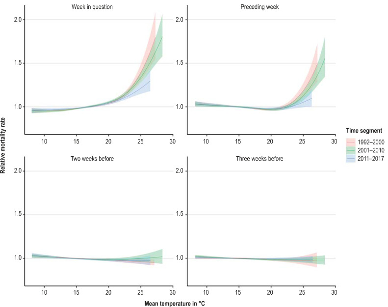
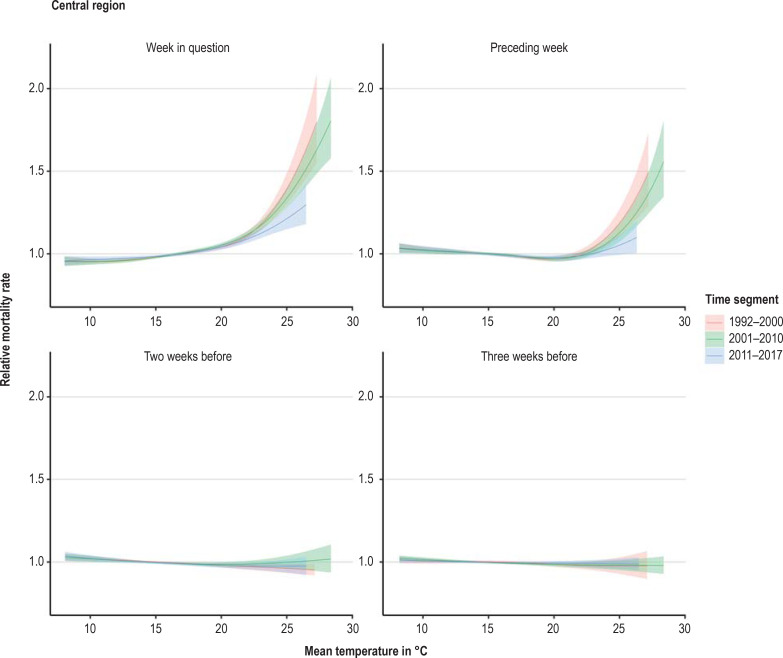
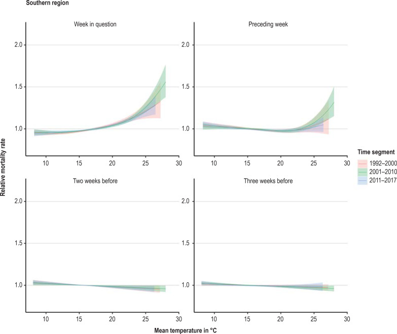
The exposure–response curve estimated in the statistical model showed a clear association of both the mean temperature of the week in question and the mean temperature of the week before with the weekly mortality rate (figure 1). The monotony of the exposure–response curve showed that there was not only a statistical association but also a dose–response effect: in each case, the relative mortality climbed higher with each increase of the weekly mean temperature above a threshold. This effect was more pronounced in older age groups and decreased over the successive time segments—with the exception of a relatively weak impact of heat in the southern region in 1992 to 2000. In the northern and central regions, taking account of this altered impact led to better adaptation of the model to the mortality data with regard to the Akaike information criterion (AIC) (29, 30). In the southern region, however, the best model adaptation resulted from a constant exposure–response curve over the whole period 1992 to 2017. Nevertheless, for the sake of enhanced comparability and further analysis of the differences we present for all three regions the model with exposure–response curves changing over time.
Figure 1.
Course of relative mortality rate (exposure–response curves) in central Germany depending on the mean temperature in the current and foregoing weeks in the age group ≥ 85 years. Data: Deaths between the 15th and 40th calendar weeks of the years 1992 to 2017
We tested for possible interactions between the mean temperatures of the week in question and the foregoing week, but this did not lead to any relevant improvement in adaptation to the mortality data with regard to the AIC or the bayesian information criterion (BIC) (29, 30). The temperature during the preceding week therefore seemed not to greatly effect the impact of temperature on mortality in the week under examination. Thus we found no evidence that especially high temperatures in the previous week increased the impact of heat in the week in question.
Short-term displacement of time of death and changes in exposure–response curve
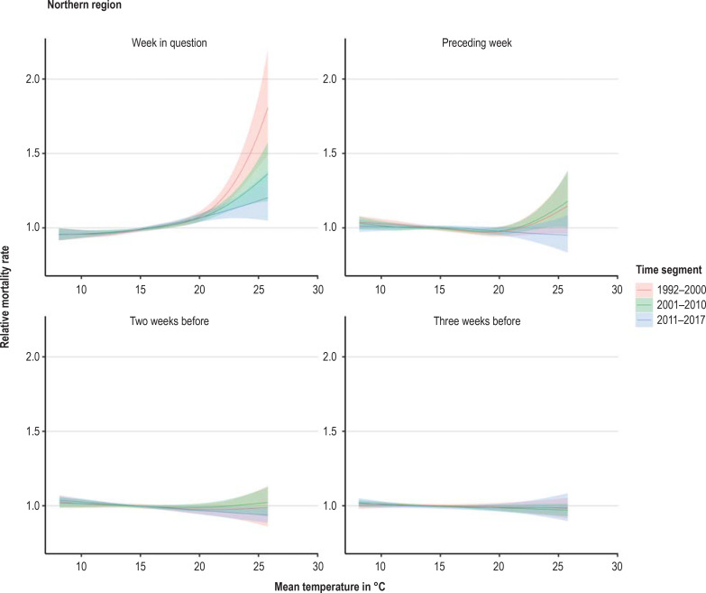
High mean temperatures 2 weeks and 3 weeks before the week in question exhibited only a minor influence on the (subsequent) mortality rate: addition of the effect of the temperature yet another week earlier led to no further improvement in model adaptation. The exposure–response curves of weeks 2 and 3 before the week concerned each showed a slightly negative effect on the mortality rate after a heatwave. This indicates that for a small proportion of deaths the time of death was merely changed by 2 or 3 weeks. For week 2 before the week in question, there was sometimes a statistically significant reduction in mortality of up to 6% (Figure 1, eFigure 2a – c). For week 3 beforehand there were no statistically significant decreases: the point estimators were up to 4% or lower. In contrast, the mortality rates in the age group ≥ 85 years in the week in question increased by up to 110% over the years 1992 to 2000 (95% confidence interval [65%; 170%]), up to 79% in 2001 to 2010 [57%; 105%], and up to 43% in 2011 to 2017 [21%; 70%]. In each time segment the highest increase was in the central region.
eFigure 2a.
Course of relative mortality rate (exposure–response curves) in northern Germany depending on the mean temperature in the current and foregoing weeks in the age group ≥ 85 years. Data: Deaths between the 15th and 40th calendar weeks of the years 1992 to 2017
eFigure 2b.
Course of relative mortality rate (exposure–response curves) in central Germany depending on the mean temperature in the current and foregoing weeks in the age group ≥ 85 years. Data: Deaths between the 15th and 40th calendar weeks of the years 1992 to 2017
Definition of a heatwave by means of threshold values
The weekly mean temperature of the week in question and the preceding week were relatively closely correlated with one another (average correlation in the summer weeks: 70%); therefore, they tended to show opposing trends in the exposure–response curve. Only from a certain temperature upwards did they both lead to an increase in the mortality rate. This temperature thus seems an apt threshold for definition of a heatwave. Comparison of threshold values obtained in this way by age group and region (provided the exposure–response curve for the mean temperature of the previous week did not have a monotonic course and thus exhibited a local minimum) revealed that the threshold was lower for older age groups and also decreased from south to north. For example, the threshold for the ≥ 85 years age group was 19.0 °C in the northern, 19.8 °C in the central, and 20.3 °C in the southern region of Germany. This reflected the higher sensitivity of older persons to heat and simultaneously showed that typically warmer regions have a higher threshold for heat (etable 1).
Estimating the number of heat-related deaths
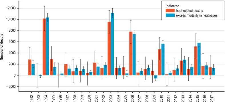
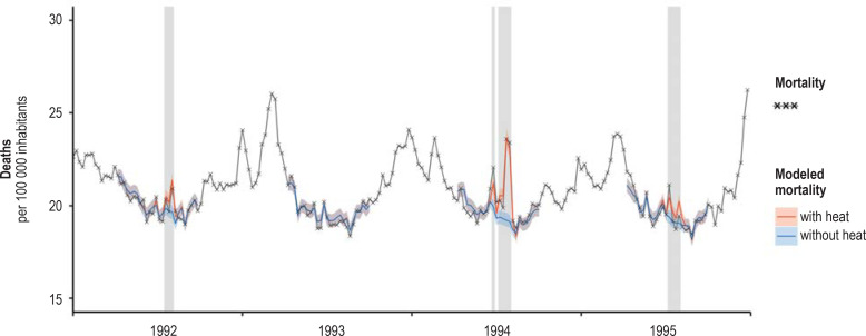
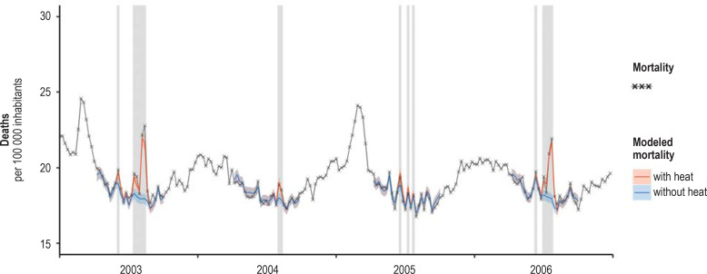
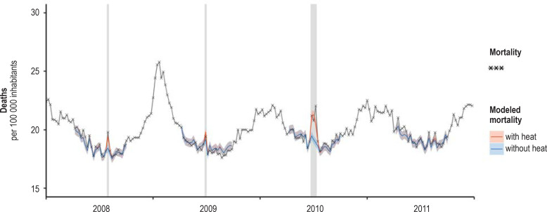
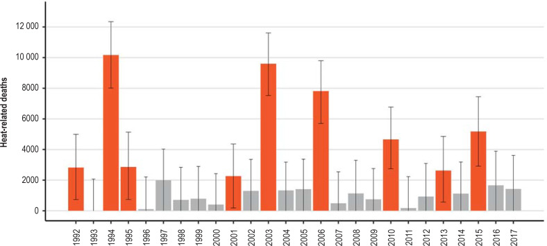
The strongest effects were exerted by the heatwaves in 1994, with approximately 10 200 heat-related deaths, and in 2003, when the number was around 9600. About 7800 deaths were estimated for the summer of 2006, 4700 deaths for 2010, and 5200 deaths for 2015. The model also estimated statistically significant numbers of heat-related deaths for the years 1992, 1995, 2001, and 2013, with point estimators between 2000 and 3000 deaths in each case (Figures 2 and 3, Table, eFigures 3a – d and 4).
Figure 2.
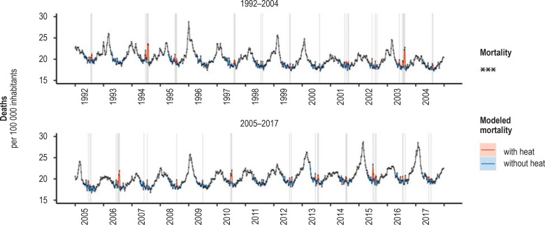
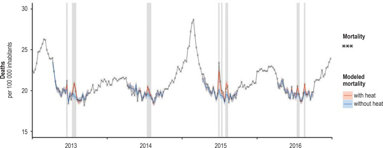
Adaptation of the statistical model to the data on weekly mortality, Germany, 1992–2017. Shading shows weeks with a mean temperature of more than 20 °C. Only the weeks in the summer half-year (calendar weeks 15 to 40) were modeled.
Figure 3.
Comparison of the estimated number of heat-related deaths (red) and excess mortality (blue) in heatwaves in Germany between 1992 and 2017
Table 1. Estimated number of heat-related deaths in Germany, 1992 to 2017*.
| Year |
Estimated number of heat-related deaths [95% confidence interval] |
| 1992 | 2800 [700; 5000] |
| 1993 | 0 [–2100; 2100] |
| 1994 | 10 200 [8000; 12 300] |
| 1995 | 2900 [700; 5100] |
| 1996 | 100 [–2100; 2200] |
| 1997 | 2000 [–200; 4000] |
| 1998 | 700 [–1300; 2800] |
| 1999 | 800 [–-1200; 2900] |
| 2000 | 400 [–1800; 2400] |
| 2001 | 2300 [200; 4400] |
| 2002 | 1300 [–700; 3400] |
| 2003 | 9600 [7500; 11 600] |
| 2004 | 1300 [–700; 3200] |
| 2005 | 1400 [–600; 3400] |
| 2006 | 7800 [5700; 9800] |
| 2007 | 500 [–1700; 2500] |
| 2008 | 1100 [–-800; 3300] |
| 2009 | 800 [–1300; 2800] |
| 2010 | 4700 [2700; 6800] |
| 2011 | 200 [–1800; 2200] |
| 2012 | 900 [–1200; 3100] |
| 2013 | 2600 [600; 4900] |
| 2014 | 1100 [–1000; 3200] |
| 2015 | 5200 [2900; 7400] |
| 2016 | 1700 [–600; 3900] |
| 2017 | 1400 [–600; 3600] |
* The years with statistically significant numbers of estimated heat-related deaths are 1992, 1994, 1995, 2001, 2003, 2006, 2010, 2013, and 2015 (bold type)
eFigure 2c.
Course of relative mortality rate (exposure–response curves) in southern Germany depending on the mean temperature in the current and foregoing weeks in the age group ≥ 85 years. Data: Deaths between the 15th and 40th calendar weeks of the years 1992 to 2017
eFigure 3a.
Adaptation of the statistical model to the data on weekly mortality, Germany, 1992–1995. Shading shows weeks with a mean temperature of more than 20 °C. Only the weeks in the summer half-year (calendar weeks 15 to 40) were modeled.
The quality of model adaptation
The quality of model adaptation can be appreciated by juxtaposing the observed excess mortality during heatwaves and the modeled number of heat-related deaths—see also the comparison of the two parameters by an der Heiden et al. (31). Figure 3 shows that the model underestimated mortality somewhat in the years 2003, 2010, and 2015, corresponded very precisely in 1994, and overestimated mortality slightly in 2006.
Discussion
By taking into account the delayed impact of heat on the mortality rate, the observed mortality over time—particularly the peaks during heatwaves—could be depicted more precisely than with the model used by an der Heiden et al. (1). In contrast, the use of interactions between the mean temperatures of the week in question and the preceding week did not lead to improved adaptation to the mortality data with regard to the information criteria AIC and BIC. This indicates that indeed only a delayed impact of the heat in the preceding week might be relevant; the influence of the mean temperature in the week in question does not seem to be strongly affected by the level of the mean temperature in the preceding week.
Consideration of different exposure–response curves for the time segments 1992 to 2000, 2001 to 2010, and 2011 to 2017 led to better depiction of the data with regard to the AIC. The influence of heat was weaker in 2011 to 2017 than in 2001 to 2010. In the segment 1992 to 2000, the greatest impact of heat for the week in question was seen in the northern region of Germany and that for the preceding week in the northern and central regions. In the southern region, in contrast, the impact of heat in the segment 1992 to 2000 was similar to that in 2011 to 2017 (efigure 5). One possible reason for the relatively weak response particularly to the heatwave in the summer of 1994 is that this heatwave with peak temperatures reached at the end of July had been preceded in the southern region by similar peak temperature values at the end of June, leading to a better handling of the situation. In the northern and central regions, in contrast, the maximum temperatures during the heatwave in late July 1994 clearly exceeded those at the end of June.
eFigure 5.
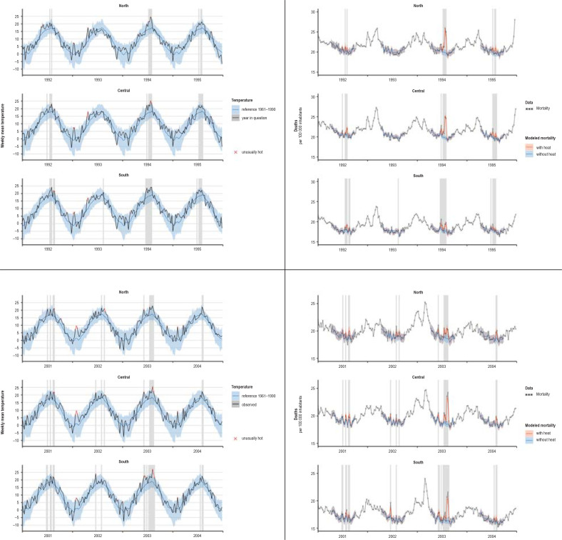
Mean temperature and modeled mortality in the northern, central, and southern regions for the heatwaves in 1994 and 2003 with adjacent years. For reference the corresponding temperature for the years 1961 to 1990 is given with 95% prediction interval. Shading shows weeks with a mean temperature of more than 20 °C. Weeks with weekly mean temperature beyond the 95% prediction interval are marked as unusually hot.
Response to heat in the southern region between 1992 and 2000
To enhance comprehension of the less pronounced response to heat in the southern region between 1992 and 2000, we look again especially at the heatwaves in 1994 and 2003. Comparing the mean temperatures in the three regions of Germany with the reference temperature (the mean for the years 1961 to 1990), it is striking that the temperatures during the 1994 heatwave in the south were still at the upper limit of the prediction interval, while in the central and northern regions they were clearly above the prediction interval. In all three regions the first peak in the temperature curve came in the last week of June. This peak is reflected in the mortality curve, before the maximum temperature in the last week of July. However, while in the south the main peak was only slight (24.2 °C, previously 23.5 °C, difference 0.7 °C), the temperatures in the central and northern regions rose much more (central: 25.1 °C versus 22.3 °C, difference 2.8 °C; north: 24.7 °C versus 19.9 °C, difference 4.8 °C).
In 2003, in contrast, the limit of the prediction interval was exceeded in central and southern Germany, while in the north the summer stayed within the normal range.
Taking into account the delayed effects of the temperature in the preceding week on mortality led to higher estimated numbers of heat-related deaths in the years 2003, 2006, and 2010. For later years, consideration of the trend in the exposure–response curve led to lower estimates overall.
Although most analyses estimate heat-related mortality on the basis of data giving the day of death, a clear systematic association is also seen when weekly data are used. Models based on precise daily data enable very accurate description of the interactions between exposure and effect, but have to be relatively complex in construction if they are to portray the interplay of the individual days (especially at the beginning of a heatwave), possible effects of the days of the week, and delays between heat exposure and death. In this regard, weekly aggregated data have the advantage of reacting immediately to the level of the heatwaves, and essentially it suffices to describe the impact on mortality of heat in the week in question and the week before.
Future studies should use similar models based on exact daily data to investigate the extent to which similar results emerge when, instead of calendar weeks, time units of between 1 and 6 days are used.
The temperature above which the exposure–response curves of the week in question and the preceding week both rise can be used as a threshold for the definition of a heatwave. It shows plausible trends with regard to age group and region. For validation of this definition, temperature thresholds derived in this way from analyses of mortality data from various parts of the world should be determined and compared.
Gasparrini et al. (26) used the thermal optimum as heatwave threshold. Using summation of delayed impacts to form the thermal optimum for the weekly analysis of the German data yielded thresholds of between 14.5 °C and 18.5 °C. These temperatures seem too low and also do not show the expected trends regarding age group and region. Thus our threshold appears more appropriate, particularly in the context of weekly data. Other studies have used, for example, the 90th percentile of the mean temperature as threshold and arrived at threshold values that are plausible but appear to have little foundation in theory (32). Hajat et al. (33) used thresholds calculated by means of simple linear threshold models and arrived at 23.4 °C for Milan, 20.5 °C for London, and 19.6 °C for Budapest.
Overall, the effect of heat on the mortality rate became weaker decade by decade over the period under consideration. This points to adjustment processes, which may rest on physiological adaptation (34), but are probably due above all to behavioral changes subsequent to the experience with earlier heatwaves and as a reaction to heat warnings and other preventive measures, which have been put in place particularly to protect the elderly. Such an effect has also been observed in other countries. Fouillet et al. (36) attributed the decreased excess mortality in France after 2003 partly to preventive measures implemented in the framework of the nationwide heat action plan instituted in 2004. In Switzerland, too, comparisons have shown less pronounced effects of high summer temperatures on the risk of death since 2003, again attributed to the introduction of heat warning systems (37). A study in Japan (38) found adaptation of the population to recent heatwaves over an extended period (1972–2010).
Most European countries have installed a heat-health action plan for overall coordination of the measures implemented after a heat warning (39). In Germany, only a small number of the federal states (e.g., Hesse) have enacted such plans. In contrast to other European nations, heat-health action plans seem to be perceived as primarily a matter for local government, with no need for state- or nationwide coordination (40). At the federal level, the Deutscher Wetterdienst provides heat warnings for individual districts.
Supplementary Material
eMethods
Modeling
We modeled the observed weekly number of deaths as a negative binomial distribution with overdispersion parameter. This parameter regulates the size of the variance in dependence of the expected value of the distribution. We used a generalized additive model (e1) to describe the non-linear effect of the weekly mean temperature (mean temperature) on the mortality rate. Additional terms were used to explicitly model the delay of this effect by up to 3 weeks. To describe any change in the impact of heatwaves on mortality, we estimated separate exposure–response curves for three segments of the period concerned: 1992 to 2000, 2001 to 2010, and 2011 to 2017.
The model equation for the observed number of deaths ![]() and its modeled expected value
and its modeled expected value ![]() took account of (a) the age groups, (t) the week in question, (wt) the calendar week, (pt) the observation period,
took account of (a) the age groups, (t) the week in question, (wt) the calendar week, (pt) the observation period, ![]() the population size, and (mt) the weekly mean temperature. The following then applied to each of the regions independently:
the population size, and (mt) the weekly mean temperature. The following then applied to each of the regions independently:
The smooth functions were selected as penalized B-splines (“P-splines”). The functions  and
and ![]() modeled the yearly periodicity and the long-term trend of age-specific mortality. To avoid fluctuation of the trend, no more than one degree of freedom for each 2 years of observation was permitted. Thus, a maximum of 13 degrees of freedom were possible for the period 1992 to 2017.
modeled the yearly periodicity and the long-term trend of age-specific mortality. To avoid fluctuation of the trend, no more than one degree of freedom for each 2 years of observation was permitted. Thus, a maximum of 13 degrees of freedom were possible for the period 1992 to 2017.
The functions  modeled the non-linear influence of the mean temperature of the week in question (i=0) and the preceding 3 weeks (i=1, 2, 3) on the mortality rate. This influence varied among the age groups and among the time segments (pt). The number of degrees of freedom for temperature dependency was limited to eight, especially in order to ensure a stable association at the extremes of the temperature range. No limitation was imposed on the numbers of degrees of freedom for the seasonal components.
Based on the results of the model we determined a heatwave using a threshold weekly mean temperature. This threshold was defined by us as the weekly mean temperature above which the exposure–response curves of the week in question and the preceding week both rise. We had to consider that, of course, a definition in terms of, say, a threshold daily mean temperature would have led to somewhat different heatwaves. We estimated the number of heat-related deaths as the difference between the modeled number of deaths and the hypothetical number of deaths for a temperature course that did not exceed the selected threshold but remained constant at that level until the end of the heatwave (capped mean temperature).
The quality of model adaptation can be assessed by comparing the modeled number of heat-related deaths with the observed excess mortality during heatwaves. We estimated the latter as the difference between observed deaths and the hypothetical course of modeled mortality for the capped mean temperature.
Maximum number of degrees of freedom in the spline components of the model
The outcome of model adaptation was effectively that far fewer degrees of freedom were used in all spline components, suggesting that a stable solution had been found within the predetermined framework.
Estimating the number of heat-related deaths from data on overall mortality
In principle, peaks in the numbers of deaths over time coinciding with heatwaves could be explained by factors other than “additional” deaths (i.e., deaths that would not have occurred in the following few weeks without exposure). The heat might systematically lead to slight advancement of the time of death. This, however, would result in decreased mortality after the end of the heatwave. To a certain extent we found evidence for such an effect in the exposure–response curves for weeks 2 and 3 before the week in question. We took account of this small decrease in mortality when estimating the number of heat-related deaths.
Theoretically, these small-scale advancements of the time of death could persist for many months after the end of the heatwave. In our view, however, it seems biologically implausible that a heatwave causes such forward displacement of the time of death by a few days not only in the days and weeks immediately thereafter but also in the following fall or winter—and in such a way that the overall mortality figures show excess mortality only directly after the heatwave, with no systematic excess or decreased mortality at any later time.
Armstrong et al. (e2) have shown that in various studies heatwaves led to an increase in the overall number of deaths over a 12-month period (always beginning in May) that corresponded to the greater part of the acute excess mortality at the time of the high temperatures. This cannot be explained by slight advancement of the time of death in the summer months. For this reason, altogether it seems biologically implausible that the observed excess mortality is essentially caused by such forward displacement.
Estimating shortening of life span due to heatwaves
Adjustment for the pre-existing comorbidities of the deceased persons when estimating the shortening of life span due to heatwaves is plainly only possible when the comorbidities are known. This was, however, not the case, because only overall mortality was analyzed. Even taking cause of death records into account would have provided only an incomplete solution.
The estimated number of heat-related deaths therefore cannot simply be added to separate estimates of deaths from other causes.
Key Messages.
The heatwaves in 1994 and 2003 had the greatest impact, with around 10 000 deaths in each year. Around 8000 deaths are estimated for the summer of 2006, and for the the years 2010 and 2015 approximately 5000 deaths.
The model also estimates statistically significant numbers of heat-related deaths for 1992, 1995, 2001, and 2013, with a point estimate between 2000 and 3000 deaths for each of these four years.
The effect of heat on mortality decreases over the decades under consideration. This suggests that adaptive processes have occurred: apart from physiological adaptation, these comprise in particular behavioral changes subsequent to the experience with earlier heatwaves and as a reaction to heat warnings and other preventive measures, which have been put in place particularly to protect the elderly.
The resolution of weekly data is sufficient to estimate heat-related deaths and to allow for a definition of heat waves by means of a threshold when the weekly mean temperature is surpassed.
The mean temperature of the preceding week does not seem to alter the effect of the mean temperature of the current week on mortality. Thus, we did not find evidence that high temperatures in the preceding week lead to a stronger effect of heat in the current week.
eFigure 3b.
Adaptation of the statistical model to the data on weekly mortality, Germany, 2003–2006. Shading shows weeks with a mean temperature of more than 20 °C. Only the weeks in the summer half-year (calendar weeks 15 to 40) were modeled.
eFigure 3c.
Adaptation of the statistical model to the data on weekly mortality, Germany, 2008–2011. Shading shows weeks with a mean temperature of more than 20 °C. Only the weeks in the summer half-year (calendar weeks 15 to 40) were modeled.
eFigure 3d.
Adaptation of the statistical model to the data on weekly mortality, Germany, 2013–2016. Shading shows weeks with a mean temperature of more than 20 °C. Only the weeks in the summer half-year (calendar weeks 15 to 40) were modeled.
eFigure 4.
Estimated number of heat-related deaths in Germany, 1992–2017. The years with a statistically significant estimated number of heat-related deaths are 1992, 1994, 1995, 2001, 2003, 2006, 2010, 2013, and 2015 (in red).
eTable 2. Heat threshold and thermal optimum by region and age group (mean for the segments 1992–2000, 2001–2010, and 2011–2017)*.
| Age group | ||||
| Region | < 65 | 65–74 | 75–84 | 85+ |
| Thermal optimum | ||||
| Northern | 15.1 | 16.4 | 16.9 | 16.0 |
| Central | 17.4 | 18.3 | 18.5 | 17.3 |
| Southern | 14.5 | 17.6 | 17.5 | 17.2 |
| Heat threshold | ||||
| Northern | – | – | 19.2 | 19.0 |
| Central | 20.9 | 20.4 | 20.0 | 19.8 |
| Southern | – | 20.8 | 20.5 | 20.3 |
* For some combinations no threshold for heat can be determined, because the corresponding exposure–response curve for the mean temperature of the preceding week is monotonic and therefore features no local minimum.
Acknowledgments
Translated from the original German by David Roseveare
Footnotes
Conflict of interest statement The authors declare that no conflict of interest exists.
References
- 1.an der Heiden M, Muthers S, Niemann H, Buchholz U, Grabenhenrich L, Matzarakis A. Schätzung hitzebedingter Todesfälle in Deutschland zwischen 2001 und 2015. Bundesgesundheitsblatt Gesundheitsforschung Gesundheitsschutz. 2019;62:571–579. doi: 10.1007/s00103-019-02932-y. [DOI] [PubMed] [Google Scholar]
- 2.Kovats RS, Kristie LE. Heatwaves and public health in Europe. Eur J Public Health. 2006;16:592–599. doi: 10.1093/eurpub/ckl049. [DOI] [PubMed] [Google Scholar]
- 3.Mora C, Dousset B, Caldwell IR, et al. Global risk of deadly heat. Nat Clim Chang. 2017;7:501–506. [Google Scholar]
- 4.Muthers S, Laschewski G, Matzarakis A. The summers 2003 and 2015 in South-West Germany: Heat waves and heat-related mortality in the context of climate change. Atmosphere. 2017;8 [Google Scholar]
- 5.Steul K, Schade M, Heudorf U. Mortality during heatwaves 2003-2015 in Frankfurt-Main—the 2003 heatwave and its implications. Int J Hyg Environ Health. 2018;221:81–86. doi: 10.1016/j.ijheh.2017.10.005. [DOI] [PubMed] [Google Scholar]
- 6.Flynn A, McGreevy C, Mulkerrin E. Why do older patients die in a heatwave? Qjm. 2005;98:227–229. doi: 10.1093/qjmed/hci025. [DOI] [PubMed] [Google Scholar]
- 7.Hajat S, Kovats RS, Lachowycz K. Heat-related and cold-related deaths in England and Wales: who is at risk? Occup Environ Med. 2007;64:93–100. doi: 10.1136/oem.2006.029017. [DOI] [PMC free article] [PubMed] [Google Scholar]
- 8.Russo S, Sillmann J, Fischer EM. Top ten European heatwaves since 1950 and their occurrence in the coming decades. Environ Res Lett. 2015;10 [Google Scholar]
- 9.Otto FE, Massey N, Van Oldenborgh G, Jones R, Allen M. Reconciling two approaches to attribution of the 2010 Russian heat wave. Geophys Res Lett. 2012 [Google Scholar]
- 10.Sippel S, Otto FE, Flach M, van Oldenborgh GJ. The role of anthropogenic warming in 2015 central European heat waves. Bull Am Meteorol Soc. 2016;97:S51–S56. [Google Scholar]
- 11.Stott PA, Stone DA, Allen MR. Human contribution to the European heatwave of 2003. Nature. 2004;432:610–614. doi: 10.1038/nature03089. [DOI] [PubMed] [Google Scholar]
- 12.Christidis N, Jones GS, Stott PA. Dramatically increasing chance of extremely hot summers since the 2003 European heatwave. Nat Clim Chang. 2015;5 [Google Scholar]
- 13.Fischer EM, Schär C. Future changes in daily summer temperature variability: driving processes and role for temperature extremes. Climate Dynamics. 2009;33 [Google Scholar]
- 14.Guerreiro SB, Dawson RJ, Kilsby C, Lewis E, Ford A. Future heat-waves, droughts and floods in 571 European cities. Environ Res Lett. 2018;13 034009. [Google Scholar]
- 15.Lhotka O, Kyselý J, Farda A. Climate change scenarios of heat waves in Central Europe and their uncertainties. Theor Appl Climatol. 2018;131:1043–1054. [Google Scholar]
- 16.Nowak D. Global warming—the German picture. Dtsch Arztebl Int. 2019;116:519–520. doi: 10.3238/arztebl.2019.0519. [DOI] [PMC free article] [PubMed] [Google Scholar]
- 17.Watts N, Adger WN, Agnolucci P, et al. Health and climate change: policy responses to protect public health. Lancet. 2015;386:1861–1914. doi: 10.1016/S0140-6736(15)60854-6. [DOI] [PubMed] [Google Scholar]
- 18.World Health Organisation. WHO calls for urgent action to protect health from climate change. www.who.int/globalchange/global-campaign/cop21/en/ (last accessed on 29 January 2020) [Google Scholar]
- 19.Campbell-Lendrum D, Manga L, Bagayoko M, Sommerfeld J. Climate change and vector-borne diseases: what are the implications for public health research and policy? Philos Trans R Soc Lond B Biol Sci. 2015;370 doi: 10.1098/rstb.2013.0552. 20130552. [DOI] [PMC free article] [PubMed] [Google Scholar]
- 20.Ogden NH. Climate change and vector-borne diseases of public health significance. FEMS Microbiol Lett. 2017;364 doi: 10.1093/femsle/fnx186. doi: 10.1093/femsle/fnx186. [DOI] [PubMed] [Google Scholar]
- 21.Stark K, Niedrig M, Biederbick W, Merkert H, Hacker J. Die Auswirkungen des Klimawandels. Bundesgesundheitsblatt Gesundheitsforschung Gesundheitsschutz. 2009;52:699–714. doi: 10.1007/s00103-009-0874-9. [DOI] [PubMed] [Google Scholar]
- 22.Leyk D, Hoitz J, Becker C, Glitz KJ, Nestler K, Piekarski C. Health risks and interventions in exertional heat stress. Dtsch Arztebl Int. 2019;116:537–544. doi: 10.3238/arztebl.2019.0537. [DOI] [PMC free article] [PubMed] [Google Scholar]
- 23.Eis D, Helm D, Laußmann D, Stark K. Klimawandel und Gesundheit. Ein Sachstandsbericht. Berlin: Robert Koch-Institut. 2010 [Google Scholar]
- 24.Basu R, Malig B. High ambient temperature and mortality in California: exploring the roles of age, disease, and mortality displacement. Environ Res. 2011;111:1286–1292. doi: 10.1016/j.envres.2011.09.006. [DOI] [PubMed] [Google Scholar]
- 25.Braga AL, Zanobetti A, Schwartz J. The effect of weather on respiratory and cardiovascular deaths in 12 US cities. Environ Health Perspect. 2002;110:859–863. doi: 10.1289/ehp.02110859. [DOI] [PMC free article] [PubMed] [Google Scholar]
- 26.Gasparrini A, Guo Y, Hashizume M, et al. Mortality risk attributable to high and low ambient temperature: a multicountry observational study. Lancet. 2015;386:369–375. doi: 10.1016/S0140-6736(14)62114-0. [DOI] [PMC free article] [PubMed] [Google Scholar]
- 27.Monteiro A, Carvalho V, Oliveira T, Sousa C. Excess mortality and morbidity during the July 2006 heat wave in Porto, Portugal. Int J Biometeorol. 2013;57:155–167. doi: 10.1007/s00484-012-0543-9. [DOI] [PubMed] [Google Scholar]
- 28.Zanobetti A, Wand M, Schwartz J, Ryan L. Generalized additive distributed lag models: quantifying mortality displacement. Biostatistics. 2000;1:279–292. doi: 10.1093/biostatistics/1.3.279. [DOI] [PubMed] [Google Scholar]
- 29.Akaike H. Information theory and an extension of the maximum likelihood principle. Second International Symposium on Information Theory. 1973:267–281. [Google Scholar]
- 30.Schwarz G. Estimating the dimension of a model. Ann Statist. 1978;6:461–464. [Google Scholar]
- 31.an der Heiden M, Buchholz U, Uphoff H. Schätzung der Zahl hitzebedingter Sterbefälle infolge der Hitzewelle 2018. Epidemiologisches Bulletin. 2019;23:193–197. [Google Scholar]
- 32.Scortichini M, de’Donato F, De Sario M, et al. The inter-annual variability of heat-related mortality in nine European cities (1990-2010) Environ Health. 2018;17:1–10. doi: 10.1186/s12940-018-0411-0. [DOI] [PMC free article] [PubMed] [Google Scholar]
- 33.Hajat S, Armstrong B, Baccini M, et al. Impact of high temperatures on mortality: is there an added heat wave effect? Epidemiology. 2006;17:632–638. doi: 10.1097/01.ede.0000239688.70829.63. [DOI] [PubMed] [Google Scholar]
- 34.Gekle M, Singer D, Jessen C. Klinke R, Pape H-C, Silbernagl S, editors. Temperaturregulation und Wärmehaushalt Lehrbuch Physiologie. Georg Thieme Verlag. 2005:493–508. [Google Scholar]
- 35.Matzarakis A, Laschewski G, Muthers S. The heat health warning system in Germany—application and warnings for 2005 to 2019. Atmosphere. 2020;11 [Google Scholar]
- 36.Fouillet A, Rey G, Wagner V, et al. Has the impact of heat waves on mortality changed in France since the European heat wave of summer 2003? A study of the 2006 heat wave. Int J Epidemiol. 2008;37:309–317. doi: 10.1093/ije/dym253. [DOI] [PMC free article] [PubMed] [Google Scholar]
- 37.Ragettli MS, Vicedo-Cabrera AM, Schindler C, Röösli M. Exploring the association between heat and mortality in Switzerland between 1995 and 2013. Environ Res. 2017;158:703–709. doi: 10.1016/j.envres.2017.07.021. [DOI] [PubMed] [Google Scholar]
- 38.Ng CFS, Boeckmann M, Ueda K, et al. Heat-related mortality: effect modification and adaptation in Japan from 1972 to 2010. Global environmental change. 2016;39:234–243. [Google Scholar]
- 39.Casanueva A, Burgstall A, Kotlarski S, et al. Overview of existing heat-health warning systems in Europe. Int J Environ Res Public Health. 2019;16 doi: 10.3390/ijerph16152657. [DOI] [PMC free article] [PubMed] [Google Scholar]
- 40.Blättner B, Janson D, Grewe HA. Hitzeaktionspläne in den Parlamenten der Bundesländer. Präv Gesundheitsf. 2020;15:296–302. [Google Scholar]
- E1.Wood SN. Chapman and Hall/CRC. New York: 2006. Generalized additive models: an introduction with R. [Google Scholar]
- E2.Armstrong B, Bell ML, de Sousa Zanotti Stagliorio Coelho M, et al. Longer-term impact of high and low temperature on mortality: an international study to clarify length of mortality displacement. Environ Health Perspect. 2017;125 doi: 10.1289/EHP1756. 107009. [DOI] [PMC free article] [PubMed] [Google Scholar]
Associated Data
This section collects any data citations, data availability statements, or supplementary materials included in this article.
Supplementary Materials
eMethods
Modeling
We modeled the observed weekly number of deaths as a negative binomial distribution with overdispersion parameter. This parameter regulates the size of the variance in dependence of the expected value of the distribution. We used a generalized additive model (e1) to describe the non-linear effect of the weekly mean temperature (mean temperature) on the mortality rate. Additional terms were used to explicitly model the delay of this effect by up to 3 weeks. To describe any change in the impact of heatwaves on mortality, we estimated separate exposure–response curves for three segments of the period concerned: 1992 to 2000, 2001 to 2010, and 2011 to 2017.
The model equation for the observed number of deaths ![]() and its modeled expected value
and its modeled expected value ![]() took account of (a) the age groups, (t) the week in question, (wt) the calendar week, (pt) the observation period,
took account of (a) the age groups, (t) the week in question, (wt) the calendar week, (pt) the observation period, ![]() the population size, and (mt) the weekly mean temperature. The following then applied to each of the regions independently:
the population size, and (mt) the weekly mean temperature. The following then applied to each of the regions independently:
The smooth functions were selected as penalized B-splines (“P-splines”). The functions  and
and ![]() modeled the yearly periodicity and the long-term trend of age-specific mortality. To avoid fluctuation of the trend, no more than one degree of freedom for each 2 years of observation was permitted. Thus, a maximum of 13 degrees of freedom were possible for the period 1992 to 2017.
modeled the yearly periodicity and the long-term trend of age-specific mortality. To avoid fluctuation of the trend, no more than one degree of freedom for each 2 years of observation was permitted. Thus, a maximum of 13 degrees of freedom were possible for the period 1992 to 2017.
The functions  modeled the non-linear influence of the mean temperature of the week in question (i=0) and the preceding 3 weeks (i=1, 2, 3) on the mortality rate. This influence varied among the age groups and among the time segments (pt). The number of degrees of freedom for temperature dependency was limited to eight, especially in order to ensure a stable association at the extremes of the temperature range. No limitation was imposed on the numbers of degrees of freedom for the seasonal components.
Based on the results of the model we determined a heatwave using a threshold weekly mean temperature. This threshold was defined by us as the weekly mean temperature above which the exposure–response curves of the week in question and the preceding week both rise. We had to consider that, of course, a definition in terms of, say, a threshold daily mean temperature would have led to somewhat different heatwaves. We estimated the number of heat-related deaths as the difference between the modeled number of deaths and the hypothetical number of deaths for a temperature course that did not exceed the selected threshold but remained constant at that level until the end of the heatwave (capped mean temperature).
The quality of model adaptation can be assessed by comparing the modeled number of heat-related deaths with the observed excess mortality during heatwaves. We estimated the latter as the difference between observed deaths and the hypothetical course of modeled mortality for the capped mean temperature.
Maximum number of degrees of freedom in the spline components of the model
The outcome of model adaptation was effectively that far fewer degrees of freedom were used in all spline components, suggesting that a stable solution had been found within the predetermined framework.
Estimating the number of heat-related deaths from data on overall mortality
In principle, peaks in the numbers of deaths over time coinciding with heatwaves could be explained by factors other than “additional” deaths (i.e., deaths that would not have occurred in the following few weeks without exposure). The heat might systematically lead to slight advancement of the time of death. This, however, would result in decreased mortality after the end of the heatwave. To a certain extent we found evidence for such an effect in the exposure–response curves for weeks 2 and 3 before the week in question. We took account of this small decrease in mortality when estimating the number of heat-related deaths.
Theoretically, these small-scale advancements of the time of death could persist for many months after the end of the heatwave. In our view, however, it seems biologically implausible that a heatwave causes such forward displacement of the time of death by a few days not only in the days and weeks immediately thereafter but also in the following fall or winter—and in such a way that the overall mortality figures show excess mortality only directly after the heatwave, with no systematic excess or decreased mortality at any later time.
Armstrong et al. (e2) have shown that in various studies heatwaves led to an increase in the overall number of deaths over a 12-month period (always beginning in May) that corresponded to the greater part of the acute excess mortality at the time of the high temperatures. This cannot be explained by slight advancement of the time of death in the summer months. For this reason, altogether it seems biologically implausible that the observed excess mortality is essentially caused by such forward displacement.
Estimating shortening of life span due to heatwaves
Adjustment for the pre-existing comorbidities of the deceased persons when estimating the shortening of life span due to heatwaves is plainly only possible when the comorbidities are known. This was, however, not the case, because only overall mortality was analyzed. Even taking cause of death records into account would have provided only an incomplete solution.
The estimated number of heat-related deaths therefore cannot simply be added to separate estimates of deaths from other causes.


