Brain-inspired classical conditioning model

Summary

Classical conditioning plays a critical role in the learning process of biological brains, and many computational models have been built to reproduce the related classical experiments. However, these models can reproduce and explain only a limited range of typical phenomena in classical conditioning. Based on existing biological findings concerning classical conditioning, we build a brain-inspired classical conditioning (BICC) model. Compared with other computational models, our BICC model can reproduce as many as 15 classical experiments, explaining a broader set of findings than other models have, and offers better computational explainability for both the experimental phenomena and the biological mechanisms of classical conditioning. Finally, we validate our theoretical model on a humanoid robot in three classical conditioning experiments (acquisition, extinction, and reacquisition) and a speed generalization experiment, and the results show that our model is computationally feasible as a foundation for brain-inspired robot classical conditioning.

Graphical abstract

Highlights

• •Classical conditioning (CC) is crucial in biological and embodied robot learning
• •A spiking neural network incorporates existing biological findings of CC in one model
• •BICC can explain a broader set of findings than other existing computational models
• •BICC ensures a robot gets similar biological behavior and speed generalization capability

Neuroscience; cognitive neuroscience; artifical intelligence; robotics

Introduction

Classical conditioning is regarded as a basic learning method for animals in which an association is built between a conditioned stimulus ($CS$) and a conditioned response ($CR$). The best-known experiment of classical conditioning was performed by Pavlov (1927). When a dog is presented with food (unconditioned stimulus, $US$), it will start to salivate (unconditioned response, $UR$). In Pavlov's research, a dog would hear a tone ($CS$) before being presented with food every time. After a number of trials, the dog started to salivate ($CR$) upon hearing a tone.

Computational model

Classical conditioning has attracted the interest of many researchers, and attempts have been made to build a computational model to reveal its mechanism. Rescorla and Wagner (1972) presented the first computational model of classical conditioning, which is named the Rescorla-Wanger model. This model can predict some important classical phenomena of classical conditioning, and it has led to a great deal of research, including modifications and alternative models. The Sutton-Barto (SB) model (Sutton and Barto, 1981) is a temporally refined extension of the Rescorla-Wanger model. This model learns to increase its response rate in anticipation of increased stimulation, and it can account for more phenomena observed in classical conditioning than the Rescorla-Wanger model can; furthermore, it has served as the precursor of many later models. The temporal difference (TD) model (Sutton and Barto, 1987) is an extension of the SB model. This model takes the form of a temporal difference prediction method and can successfully model the inter-stimulus interval (ISI) effect, which is regarded as a primary real-time effect of classical conditioning. Harry Klopf (1988) proposed a neuronal model that is modified from the Hebbian model to be more consistent with animal learning phenomena; this model can predict a wide range of classical conditioning phenomena. Schmajuk and DiCarlo (1992) presented a multilayer neural network called the S-D model. They mapped the nodes and connections onto regional cerebellar, cortical, and hippocampal circuits to obtain a model that can correctly describe the effects of hippocampal and cortical lesions on conditioning. Balkenius and Moren (1999) described a computational model of classical conditioning that is built on the assumption that the goal of learning is the prediction of a temporally discounted reward or punishment based on the current stimulus situation; notably, this model is well suited for robotic implementation. Johansson and Lansner (2002) presented an associative model of classical conditioning that is composed of a number of interconnected Bayesian confidence propagation neural networks (BCPNNs) implemented on the basis of Hebbian learning, and the output of this model fits the results of classical conditioning experiments. Zuo et al. (2005) introduced a spiking-neuron-based cognitive model. This model can simulate the learning process of classical conditioning with a reflex arc structure and a reinforcement learning method based on the Hebb rule, and an inverted pendulum experiment validated the effectiveness of this model. Liu et al. (2008) built a model with classical conditioning behaviors based on a Bayesian network (CRMBBN). This model constructs cause-effect relationships between classical sensing and nonclassical conditional sensing by means of a Bayesian network, and it can successfully simulate many phenomena, such as acquisition, inter-stimulus effects, and extinction. Liu and Ding (2008) presented a dynamic policy adaptation framework inspired by classical conditioning. This model can successfully realize the self-learning process of classical conditioning and achieve adaptive network policy management. Antonietti et al. (2017) developed a detailed spiking cerebellar microcircuit model that can reproduce eyeblink classical conditioning and successfully fits real experimental datasets from humans.

Here, we build a brain-inspired classical conditioning (BICC) model that integrates and adopts existing biological findings of classical conditioning. With a quaternionic-rate-based synaptic learning rule, which is equivalent to spike-timing-dependent plasticity (STDP) (Bi and Poo, 2001) on a timescale of seconds, the BICC model could predict the majority of classical conditioning phenomena. The computational model of biological classical conditioning enables a robot gets similar learning behavior and the capability of speed generalization. Furthermore, the changes in synaptic weights in this model may hint at the biological mechanism of classical conditioning.

Classical experiments

There are several classical conditioning experiments that can be used to verify the effectiveness of computational models. To enable reasonable comparisons with other well-known computational models, we follow the classical conditioning experiments outlined by Balkenius and Moren (1998). The stimulus before the $+$ presents first, and the stimulus after the $+$ presents later. The parenthesis indicates that the stimuli are presented and end simultaneously. The $\Rightarrow$ indicates the result of training. The $\to$ indicates the result of the stimulus.

Acquisition

Acquisition is the ability to establish an association between a stimulus and a response, and it is the most fundamental process in classical conditioning. In an acquisition experiment, a $CS$ is presented first and a $US$ is presented subsequently after a small time interval for several trials; then, the response will be induced when the $CS$ is presented on its own. This acquisition progress can be described as follows. For an acquisition experiment involving an eyelid response in the albino rabbit, the response level forms an S-shaped curve similar to a sigmoid function (Balkenius and Moren, 1998; Schneiderman et al., 1962).

$$CS+US\Rightarrow CS\to R$$

Inter-stimulus interval effect

The ISI effect is a primary real-time effect of classical conditioning (Sutton, 1990). The ISI represents the time interval between the presentation of the $CS$ and $US$, and it can be divided into three types (Balkenius and Moren 1999): delay conditioning A, delay conditioning B, and trace conditioning (Figure S1). In delay conditioning A, the $US$ is presented immediately when the $CS$ terminates. In delay conditioning B, the $CS$ is still present when the $US$ is presented, and the CS and US terminate simultaneously. In trace conditioning, the CS and US have fixed lengths, and the CS terminates before the onset of the US. In empirical studies conducted by Schneiderman and Gormezano (1964) and Smith et al. (1969), the ISI-CR frequency function revealed a concave-down shape during the acquisition and extinction process.

Extinction

In an extinction experiment, the acquired response will disappear gradually if only a $CS$ is presented without the subsequent $US$. The extinction process can be described as follows:

$$CR\Rightarrow CS\to noR$$

Reacquisition effect

The reacquisition effect is demonstrated when an animal relearns a previously extinguished association, and the relearning phase is faster than the initial learning phase.

Blocking

Blocking refers to the following phenomenon: when a first stimulus $C{S}_1$ has been associated with a response and a second stimulus $C{S}_2$ then is presented and ends simultaneously with $C{S}_1$, the attempt to associate the second stimulus $C{S}_2$ with the response will be blocked. Blocking experiments show that the association of a stimulus with a response is not independent of earlier learning. The blocking process can be described as follows, where the parentheses are used to indicate that $C{S}_1$ and $C{S}_2$ are presented and end simultaneously.

$$\begin{array}{ll}\hfill & C{S}_1+US\Rightarrow C{S}_1\to R\hfill \\ \hfill & \left(C{S}_1+C{S}_2\right)+US\Rightarrow C{S}_2\to noR\hfill \end{array}$$

Secondary conditioning

In a secondary conditioning experiment, $C{S}_1$ has been associated with the response induced by the $US$, and $C{S}_1$ is then used as the $US$ for $C{S}_2$ to build an association to the response. The effect of such secondary conditioning is typically weak, and $C{S}_1$ will undergo extinction, whereas $C{S}_2$ is reinforced. The secondary conditioning progress can be described as follows:

$$\begin{array}{ll}\hfill & C{S}_1+US\Rightarrow C{S}_1\to R\hfill \\ \hfill & C{S}_2+C{S}_1\Rightarrow C{S}_2\to R\hfill \end{array}$$

Conditioned inhibition

In a conditioned inhibition experiment, $C{S}_2$ and $C{S}_0$ have been associated with the response, and then a third stimulus $C{S}_1$ is presented and ends simultaneously with one of the previously conditioned stimuli $C{S}_0$ without the $US$. In the test phase, $C{S}_1$ will inhibit the ability of $C{S}_2$ to induce the response. The conditioned inhibition process can be described as follows, where the parentheses are used to indicate that the stimuli are presented and end simultaneously.

$$\begin{array}{ll}PhaseI\hfill & C{S}_2+US\hfill \\ PhaseII\hfill & C{S}_0+US\hfill \\ \hfill & \left(C{S}_0+C{S}_1\right)+noUS\hfill \\ Test\hfill & \left(C{S}_1+C{S}_2\right)\to noR\hfill \end{array}$$

Facilitation by an intermittent stimulus

Under normal acquisition conditions, the conditioning to $C{S}_1$ is weak in the case of trace conditioning due to the long ISI. Under conditions of facilitation, the conditioning to $C{S}_1$ is facilitated by an additional $C{S}_2$. The facilitation process can be described as follows:

$$\begin{array}{ll}Normal\hfill & C{S}_1+US\Rightarrow C{S}_1\to weakR\hfill \\ Facilitated\hfill & C{S}_1+C{S}_2+US\Rightarrow C{S}_1\to strongR\hfill \end{array}$$

Overshadowing

The $C{S}_1$ and $C{S}_2$ are presented and ended simultaneously under the conditions of overshadowing; the associative strength acquired by $C{S}_1$ and $C{S}_2$ are weaker than the $C{S}_1$ or $C{S}_2$ conditioned alone in the normal acquisition condition (Angulo et al., 2020). The overshadowing process can be described as follows:

$$\begin{array}{ll}Normal\hfill & C{S}_1+US\Rightarrow C{S}_1\to strongR\hfill \\ \hfill & C{S}_2+US\Rightarrow C{S}_1\to strongR\hfill \\ Overshadowing\hfill & \left(C{S}_1+C{S}_2\right)+US\Rightarrow C{S}_1\to weakR\hfill \\ \hfill & \left(C{S}_1+C{S}_2\right)+US\Rightarrow C{S}_2\to weakR\hfill \end{array}$$

Overexpectation

The $C{S}_1$ and $C{S}_2$ have been associated with the response, respectively, then the following $C{S}_1$-$CS2$ presentations result in a weight decrement (Rescorla and Wagner, 1972). The overexpectation process can be described as follows:

$$\begin{array}{ll}PhaseI\hfill & C{S}_1+US\Rightarrow C{S}_1\to R\hfill \\ PhaseII\hfill & C{S}_2+US\Rightarrow C{S}_2\to R\hfill \\ Test\hfill & \left(C{S}_1+C{S}_2\right)+US\Rightarrow weightdecrement\hfill \end{array}$$

Recovery from overshadowing

In the overshadowing experiment, the extinction of the $C{S}_1$ will lead to an increased responding to the $C{S}_2$ (Matzel et al., 1985). The recovery from overshadowing process can be described as follows:

$$\begin{array}{ll}\hfill & \left(C{S}_1+C{S}_2\right)+US\Rightarrow \left(C{S}_1+C{S}_2\right)\to weakR\hfill \\ \hfill & C{S}_2+US\Rightarrow C{S}_2\to strongR\hfill \end{array}$$

Recovery from forward blocking

In the forward blocking experiment, the extinction of the blocker $C{S}_1$ will lead to an increased response to the blocked $C{S}_2$ (PinenO et al., 2005). The recovery from forward blocking process can be described as follows:

$$\begin{array}{ll}\hfill & C{S}_1+US\Rightarrow C{S}_1\to R\hfill \\ \hfill & \left(C{S}_1+C{S}_2\right)+US\Rightarrow C{S}_2\to noR\hfill \\ \hfill & C{S}_2+US\Rightarrow C{S}_2\to R\hfill \end{array}$$

Results

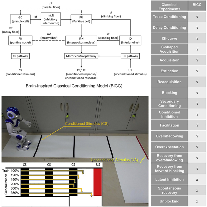
The neural circuit underlying delay eyeblink conditioning has been well described in (Hansel et al., 2001; Ten Brinke et al., 2019; Wang et al., 2018; Hogri et al., 2015; Takehara-Nishiuchi, 2018), and we propose our BICC model based on these findings. The architecture of the BICC model is shown in Figure 1.

Figure 1.

The architecture of the BICC model

The arrows and dots represent excitatory and inhibitory synapses, respectively, and the dotted lines represent excitatory or inhibitory synapses depending on the results of synaptic plasticity. The CS pathway and the US pathway are used for recognizing the CS and US through traditional pattern recognition methods and for transferring the information to the PN and IO, respectively. The PN projects the information on the CS to the IPN and GC via an mf. The IO projects the information on the US to the IPN and PU via a cf. The GC transfers the stimulus from the PN to the PU and Int.N via a pf. The PU receives inhibitory stimulation from the Int.N, excitatory stimulation from the IO via a cf, and stimulation from the GC via a pf. The IPN receives inhibitory stimulation from the PU and excitatory stimulation from the IO via a cf and from the PN via an mf. The motor control pathway receives excitatory stimulation from the IPN if the IPN is activated and then induces the CR, or it receives excitatory stimulation from the US pathway and then induces the UR.

Model evaluation

In this section, we use the changes in synaptic weight between the PN (pontine nuclei) and the IPN (interpositus nucleus) to evaluate this model; $N{P}_{C{S}_i}$ represents the neuron population of the corresponding $CS$in the PN, and $N{P}_R$ represents the neuron population that controls the response in the IPN. The PN deliver the information from the $CS$, and the IPN generates the $CR$ via the motor control pathway, as introduced in the Methods section.

Inter-stimulus interval effects

We use both delay and trace conditioning experiments to test our model, and the variation in the synaptic weight between $N{P}_{CS}$ and $N{P}_R$ is shown in Figure 2A. The curves initially show a marked increase and then exhibit a concave-down shape, which is consistent with the results of the rabbit experiment presented in Schneiderman and Gormezano (1964) and Smith et al. (1969). There is an optimal interval time for learning under every condition in this model, being 1.3 s for trace conditioning and 3.1 s for both types of delay conditioning.

Figure 2.

The results of inter-stimulus interval effects, learning curves, acquisition and extinction, and reacquisition experiments

(A) The inter-stimulus interval effects in delay and trace conditioning experiments. (1) In the delay conditioning A, the duration of the $CS$ varies from 0 to 6 s, and then the $US$ is presented immediately after the $CS$ and continues for 2 s. The ISI is equal to the length of the $CS$. (2) In the delay conditioning B, the duration of the CS varies from 1 to 7 s, whereas the $US$ continues for 1 s, and the $CS$ and $US$ end simultaneously. The ISI is equal to the difference between the length of the $CS$ and the length of the $US$. (3) In trace conditioning, the $CS$ and $US$ each continue for 2 s. The ISI is equal to the difference between the start time of the $CS$ and the start time of the $US$, and it varies from 0 to 6 s.

(B) The learning curves in the model. (1) In delay conditioning A, the $CS$ and $US$ each continue for 2 s, so the interval time is 2 s. (2) In delay conditioning B, the $CS$ continues for 3 s and the $US$ continues for 1 s, so the interval time is 2 s. (3) In trace conditioning, the $CS$ is presented at 0 s and continues for 2 s, and the $US$ is presented at 2.5 s and continues for 2 s, so the interval time is 2.5 s.

(C) The variations in synaptic weight between $N{P}_{CS}$ and $N{P}_R$. $W_{Acquisition1}$ and $W_{Acquisition2}$ represent the weight variations in the acquisition experiment when the initial weight is 0 and 0.5, respectively. $W_{Extinction}$ represents the weight variations in the extinction experiment, where there is only a $CS$.

(D) Reacquisition experiment. It is easy to see that fewer trials are needed in the reacquisition condition (fewer than 10 trials) than in the acquisition condition (approximately 25 trials) to achieve the same weight.

Learning curves

Figure 2B shows the results for the learning curves in the model. Under each condition, the curve is an S-shaped acquisition curve. With fewer than eight trials, the synaptic weight between $N{P}_{CS}$ and $N{P}_R$ is greater in the case of delay conditioning B than in the case of delay conditioning A, and the smallest weight is observed in the trace conditioning case. As the number of trials increases, the synaptic weight increases to a stable constant; ultimately, the synaptic weight under delay conditioning A is greater than that under trace conditioning, and the smallest final weight is observed in the case of delay conditioning B. We therefore select delay conditioning A for the remainder of the experiments unless otherwise stated, with both the $CS$ and the $US$ continuing for 2 s.

Acquisition, extinction, and reacquisition experiments

Figure 2C shows the variations in synaptic weight between $N{P}_{CS}$ and $N{P}_R$ in the acquisition and extinction experiments. In the acquisition experiment, the $CS$ is presented at 0 s and ends at 2 s and the $US$ is presented at 2 s and ends at 4 s. In the extinction experiment, only a $CS$ is presented at 0 s and ends at 2 s, without a $US$. The results of the reacquisition experiment are shown in Figure 2D. It is easy to see that in the reacquisition experiment, fewer trials are required to achieve a higher synaptic weight between $N{P}_{CS}$ and $N{P}_R$ than in the acquisition experiment. This is because during acquisition or extinction, not only the synaptic weight but also the number of synapses involved changes. In the reacquisition experiment, more synapses are involved in the synaptic weight changes, so the learning rate is faster than in the acquisition stage. We combine the acquisition, extinction, and reacquisition experiments into a single overall experiment. The results are shown in Figure S2.

Blocking experiment

Figure 3A shows the results of the blocking experiment. It is easy to see that the synaptic weight between $N{P}_{C{S}_2}$ and $N{P}_R$ is too small to induce a response. In the blocking stage, the changes in single synaptic weights between $N{P}_{C{S}_1}$ and $N{P}_R$ and between $N{P}_{C{S}_2}$ and $N{P}_R$ are identical because of the synchronization of $C{S}_1$ and $C{S}_2$, but there are many more synapses involved in $N{P}_{C{S}_1}$ than in $N{P}_{C{S}_2}$, which causes the change in $W_{R,C{S}_1}$ to be much greater than that in $W_{R,C{S}_2}$.

Figure 3.

The results of blocking, secondary conditioning, conditioned inhibition, and facilitation experiments

(A) Blocking experiment. In the first 10 trials, only $C{S}_1$ and $US$ are presented to build a conditioned response. In the remainder of the trials, $C{S}_1$ and $C{S}_2$ are presented and end simultaneously, and then the $US$ is presented subsequently.

(B) Secondary conditioning experiment. In the first 25 trials, $C{S}_1$ is presented first and $US$ is presented subsequently, as in the normal acquisition experiment. In the last 25 trials, $C{S}_1$ is treated as the unconditioned stimulus and is presented after $C{S}_2$.

(C) Conditioned inhibition experiment. In the first 25 and second set of 25 trials, $C{S}_2$ and $C{S}_0$, respectively, are combined with $US$ for conditioning on the response. In the subsequent 25 trials, $C{S}_0$ and $C{S}_1$ are presented and end simultaneously, without $US$. In the last 25 trials, only $C{S}_1$ and $C{S}_2$ are presented.

(D) Facilitation experiment. $C{S}_1$ continues for 2 s, $C{S}_2$ continues for 3 s, and the $US$ continues for 1 s. During normal acquisition, $C{S}_1$ is presented first, and 2 s later, the $US$ is presented. During facilitated acquisition, $C{S}_1$ is presented first, $C{S}_2$ is presented immediately when $C{S}_1$ ends, and 2 s after $C{S}_1$ ends, the $US$ is presented. $C{S}_2$ and the $US$ end simultaneously.

Secondary conditioning experiment

Figure 3B shows the results of the secondary conditioning experiment. Here, $C{S}_1$ is treated as the $US$ to build an association between $C{S}_2$ and the response, and the corresponding synaptic weight is typically weak because the synaptic weight between $N{P}_{CS1}$ and $N{P}_R$ exhibits an extinction effect at the same time.

Conditioned inhibition experiment

Figure 3C shows the results of the conditioned inhibition experiment. In the first and second sets of 25 trials, excitatory synapse connections to $N{P}_R$ are built for $N{P}_{C{S}_2}$ and $N{P}_{C{S}_0}$, respectively. In the third set of 25 trials, $N{P}_{C{S}_0}$ exhibits an extinction effect, whereas$N{P}_{C{S}_1}$ builds inhibitory synapse connections to $N{P}_R$ because of synchronism. In the last 25 trials, the number of synapses between $N{P}_{C{S}_1}$ and $N{P}_R$ increase because of the inhibitory connections and the negative weight changes. At the beginning of the last set of 25 trials, the inhibition effect from $C{S}_1$ is not sufficient to completely inhibit the excitatory input from $C{S}_2$, so $C{S}_2$ can still induce the response. With the enhancement of the inhibition effect from $C{S}_1$, at the end of the last set of 25 trials, $C{S}_1$ can inhibit the response induced by $C{S}_2$. In the extinction experiment, more than 50 trials are needed for $C{S}_2$ to lose the ability to induce the response, whereas in the conditioned inhibition experiment, fewer than 25 trials are needed because of the inhibition effect from $C{S}_1$.

Facilitation experiment

Figure 3D shows the results of the facilitation experiment. It is easy to see that the synaptic weight between $N{P}_{C{S}_1}$ and $N{P}_R$ is stronger under facilitated acquisition than under normal acquisition. Under normal acquisition, the synaptic weight is weak because of the long ISI. Under facilitated acquisition, $C{S}_2$ is conditioned on the response, and the response will be induced twice, by $C{S}_2$ and the $US$, thus causing $C{S}_1$ to build stronger synaptic connections.

Overshadowing experiment

Figure 4A shows the results of the overshadowing experiment. The synaptic weights between $N{P}_{C{S}_1}$ and $N{P}_R$ and $N{P}_{C{S}_2}$ and $N{P}_R$ are identical because of the synchronization of $C{S}_1$ and $C{S}_2$. It is easy to see that the synaptic weight in the overshadowing condition is weaker than that in the normal acquisition condition. In the overshadowing condition, the $N{P}_R$ is stimulated by $C{S}_1$ and $C{S}_2$ simultaneously, and they contribute equally to build an association to response. So, the synaptic weight in the overshadowing condition is weaker, and it is about half of that in the normal acquisition condition.

Figure 4.

The results of overshadowing, overexpectation, recovery from overshadowing, and recovery from forward blocking experiments

(A) Overshadowing experiment. In the normal acquisition condition, the $C{S}_1$ and $C{S}_2$ build a conditioned response with the $US$. In the overshadowing condition, the $C{S}_1$ and $C{S}_2$ are presented and end simultaneously and then the $US$ is presented subsequently. The dotted line shows the weight changing in the normal acquisition condition. The solid line shows the weight changing in the overshadowing condition.

(B) Overexpectation experiment. In the first 25 trials, the $C{S}_1$ is presented first and the $US$ is presented subsequently. In the subsequent 25 trials, the $C{S}_2$ is presented first and the $US$ is presented subsequently. In the last 25 trials, the $C{S}_1$ and $C{S}_2$ are presented and end simultaneously, and then the $US$ is presented subsequently.

(C) Recovery from overshadowing experiment. The first 25 trials are the overshadowing process, the $C{S}_1$ and $C{S}_2$ are presented and end simultaneously, and then the $US$ is presented subsequently. The last 25 trials are the recovery process, the $C{S}_1$ is ended, and the $C{S}_2$ presented first and the $US$ is presented subsequently.

(D) Recovery from forward blocking experiment. The first 30 trials are the blocking process. In the first 10 trials, the $C{S}_1$ is presented first and the $US$ is presented subsequently. In the subsequent 20 trials, the $C{S}_1$ and $C{S}_2$ are presented and end simultaneously, and then the $US$ is presented subsequently. The last 20 trials are the recovery process, wherein the $C{S}_1$ is ended, and the $C{S}_2$ presented first and the $US$ is presented subsequently.

Overexpectation experiment

Figure 4B shows the results of the overexpectation experiment. The synaptic weight between $N{P}_{C{S}_1}$ and $N{P}_R$ and $N{P}_{C{S}_2}$ and $N{P}_R$ have decreased in the last 25 trials, and it provided that the following $C{S}_1$-$CS2$ presentations result in a weight decrement. In the first and subsequent 25 trials, the $C{S}_1$ and $C{S}_2$ build a $CR$ with US, respectively. In the last 25 trials, the $C{S}_1$ and $C{S}_2$ stimulate the $N{P}_R$ simultaneously. So, the firing rate of the response neuron increases faster and lasts longer, and it makes an extinction effect until the model is stable again.

Recovery from overshadowing experiment

Figure 4C shows the results of the recovery from overshadowing experiment. The synaptic weight between $N{P}_{C{S}_2}$ and $N{P}_R$ has increased when the $C{S}_1$ ended, and it provided that the extinction of the $C{S}_1$ will lead to an increased respondse to the $C{S}_2$. The $N{P}_R$ is only stimulated by $C{S}_2$ when the $C{S}_1$ ended, and there is an acquisition effect when the $US$ is presented.

Recovery from forward blocking experiment

Figure 4D shows the results of the recovery from forward blocking experiment. The synaptic weight between $N{P}_{C{S}_2}$ and $N{P}_R$ has increased when the $C{S}_1$ ended, and it provided that the extinction of the blocker $C{S}_1$ will lead to an increased response to the blocked $C{S}_2$. Similar to the recovery from overshadowing experiment, the $N{P}_R$ is only stimulated by $C{S}_2$ when the $C{S}_1$ ended, and there is an acquisition effect when the $US$ is presented.

The results of the presented model in the various experiments and the comparison results with existing models are summarized in Table 1.

Table 1.

Comparison results with existing models

Classical experiments	SB	TD	Klopf	SD	Balkenius	BCPNN	CRMMBBN	Liu	BICC
Trace conditioning	∗	∗	∗	∗	∗	∗	–	–	∗
Delay conditioning	–	∗	o	∗	∗	∗	–	–	∗
ISI curve	–	∗	o	∗	o	o	–	–	∗
S-shaped acquisition	–	–	∗	–	∗	∗	–	–	∗
Acquisition	∗	∗	∗	∗	∗	∗	∗	∗	∗
Extinction	∗	∗	∗	∗	∗	∗	∗	∗	∗
Reacquisition	–	–	o	∗	–	–	∗	∗	∗
Blocking	∗	∗	∗	∗	∗	∗	–	∗	∗
Secondary conditioning	o	o	∗	–	∗	∗	–	∗	∗
Conditioned inhibition	∗	∗	∗	∗	∗	∗	–	–	∗
Facilitation	∗	∗	∗	∗	∗	o	–	–	∗
Overshadowing	–	–	∗	∗	∗	–	–	–	∗
Overexpectation	–	–	∗	–	–	–	–	–	∗
Recovery from overshadowing	–	–	–	–	–	–	–	–	∗
Recovery from forward blocking	–	–	–	–	–	–	–	–	∗
Latent inhibition	–	–	–	–	–	–	–	–	–
Spontaneous recovery	–	–	–	–	–	–	–	–	–
Unblocking	–	–	–	–	–	–	–	–	–

This table is adapted from Johansson and Lansner (2002) and Balkenius and Moren (1998). An ∗ means that the model could reproduce the correlation feature, o means that the model could reproduce partially, and - means that it is not mentioned or was unable to reproduce.

SB (Sutton and Barto 1981), TD (Sutton and Barto 1987), Klopf (Harry Klopf 1988), SD (Schmajuk and DiCarlo 1992), Balkenius (Balkenius and Moren 1999), BCPNN (Johansson and Lansner 2002), CRMBBN (Liu et al., 2008), Liu (Liu and Ding 2008).

Robotic classical conditioning experiments

We use acquisition, extinction, and reacquisition experiments and speed generalization experiment to evaluate this model on a humanoid robot.

Acquisition, extinction, and reacquisition experiments

We selected three classical conditioning experiments—acquisition, extinction, and reacquisition—to evaluate this model on a humanoid robot. A red robot was used as the participant robot, and the various stimuli used in the experiments are shown in Figure 5A. We use template matching to identify different stimuli. The sequences of stimuli in these experiments are shown in Figure 5B. In the acquisition experiment, the participant robot first was shown a red fist toy ($CS$), then was shown a blue robot ($US$), and subsequently took an avoidance action ($UR$). After learning, the participant robot would take an avoidance action ($CR$) when it saw the red fist toy ($CS$). In the extinction experiment, only the $CS$was presented; after several trials, the participant robot did not perform the $CR$ upon seeing the red fist toy ($CS$). In the reacquisition experiment, the participant robot could establish the $CR$ in fewer trials than in the acquisition experiment. The experimental results are shown in Figures 5C and 5D.

Figure 5.

The acquisition, extinction, and reacquisition experiments on humanoid robot

(A) The stimuli used in the experiments. (a) The blue robot is an unconditioned stimulus that can be regarded as the participant robot's natural enemy; therefore, the participant robot will take an avoidance action upon seeing the blue robot. (b) The red fist toy is a conditioned stimulus. (c) The yellow duck is an interference stimulus used to prove that only the learned stimulus can induce the response. (d) Nothing detected means that there is no stimulus.

(B) The sequences of stimuli for acquisition (upper) and extinction (below).

(C and D) (C) Dynamic changes of weight in robotic classical conditioning experiments. (D) Dynamic changes of response in robotic classical conditioning experiments. The red line indicates the response threshold. The total number of trials is 16, consisting of 3 acquisition trials, 8 extinction trials, 1 reacquisition trial, and 2 extinction trials in addition to 2 interference stimuli (in trials 4 and 7) in the first extinction experiment.

Speed generalization experiment

The speed generalization experiment is that the robot trained at a slow speed on a navigation task; then it could navigate the track at a higher speed without training (Herreros et al., 2013). The humanoid robot Nao is a biped robot. According to its documentation, the speed parameter is the fraction of the maximum speed, such as 100% means the full speed. According to our verification, may be due to the aging problem, the robot cannot move accurately at a given speed, and often deviates from the direction when walking in a straight line. So, we test the speed generalization capabilities of the model in both real and simulation environments.

The real environment is shown as Figure 6A. In the real environment, the robot is trained at 50% speed and tested at 100% speed. We use simple image recognition algorithms to recognize the CS (black line, Figure 6B) and the US (red line, Figure 6C). For the black line recognition, we retain the central area of the image, then convert the image to a binary image according to the given threshold value, delete the small-area object, and finally perform horizontal line detection to complete the recognition. For the red line recognition, we extract the matching color area by setting the threshold value and then detect the horizontal line to complete the recognition. The result of the real environment is shown as Figure 7.

Figure 6.

Speed generalization experiment in real environment

(A) The real environment. The white runway is the track for the robot to navigate. The red line is the US, which means the robot needs to turn right to avoid leaving the runway, and the black line is the CS.

(B) The CS perceived in robot vision.

(C) The US perceived in robot vision.

Figure 7.

The result of speed generalization experiment in real environment

(A–D) The $V_{CR}$ is the firing rate of response neuron when it receives CS. For easy comparison, we show the firing rate of response neuron when it receives only US ($V_{UR}$). The red line indicates the response threshold. Compared with (A and B), with the increase of speed, the density of CS increased, so the $V_{CS}$ is stronger. (C) The firing rate of CR and UR at 50% speed. It is easy to see that after training, the robot could perform CR before UR. (D) The firing rate of CR and UR at 100% speed. It is easy to see that without training, the robot could perform CR before UR.

The simulation environment is shown as Figure 8A. In the simulation environment, we use two experiments to test the speed generalization capacity of the model. In the first experiment, we test the induced time of CR and UR at a given speed in the range of 100%–200% with 10% speed increments. The result is shown as Figure 8B. In the second experiment, we test the induced distance of CR at a given speed at 100%, 120%, 150%, 200%, 300%, 350%, and 400%. The result is shown as Figure 8C. And if the speed is greater than 350%, the robot experiment fails.

Figure 8.

Speed generalization experiment in simulation environment

(A) Simulation environment. The black square is the CS, and the red square is the US. The US indicates that the robot should turn right to avoid leaving the runway.

(B) The induced time of CR and UR at different speeds. It easy to see that the robot could perform CR before UR.

(C) The induced distance of CR at different speeds. The robot successfully passed the experiment with a maximum speed of 350%. When the speed reached 400%, the CS could not induce the CR, and the experiment failed.

The results of real and simulation environments show that the proposed model has the capacity of speed generalization.

Discussion

The BICC model exhibits long-term depression (LTD) at GC (granule cell)-PU (Purkinje cell) synapses and long-term potentiation (LTP) at PN-IPN synapses, which is consistent with the findings from electrophysiological experiments on eyeblink conditioning presented in Koekkoek et al. (2003) and Steuber et al. (2007) and Pugh and Raman, (2006, 2008), respectively. LTD is also exhibited at PN-IPN synapses in this model, representing another mechanism of synaptic plasticity that is consistent with the electrophysiological experiments reported in Zhang and Linden (2006), but there have been fewer reports of this mechanism than of the former.

LTD at GC-PU synapses

If only the $CS$ is presented before learning, the GC (granule cell) receives the $CS$ from the PN and then projects it to an Int.N (inhibitory interneuron). The inhibitory input from the Int.N will inhibit the excitatory input from the GC and the spontaneous firing of the PU, so the firing rate of the PU will immediately drop to zero; in other words, the firing of the PU will be paused. The synaptic weight between the GC and PU will not change because the postsynaptic neurons in the PU is not fired.

If only the $US$ is presented before learning, the $US$ is projected to the motor control pathway and induces the $UR$. In parallel, the IO (inferior olive) receives the $US$ from the US pathway and then projects it to the IPN and PU via the cf (climbing fiber). The excitatory input from the IO to the PU will enhance the inhibition from the PU to the IPN. The synaptic weight between the GC and PU remains unchanged because the presynaptic neuron in the GC is not fired.

In the acquisition experiment, the firing rate of the PU will gradually decay to zero because of the additional excitatory input from the $US$. With the increased firing rate of the presynaptic neurons in the GC and the decreasing firing rate of the postsynaptic neurons in the PU, the synaptic weight between the GC and PU will decrease and exhibit LTD. An intuitive explanation of how spike-based STDP can influence synaptic efficiency through a rate-based mechanism can be found in Bengio et al. (2017). In short, the synaptic weight is updated in proportion to the product of the presynaptic firing rate and the temporal rate of change in activity on the postsynaptic side. The synaptic weight is updated in our model based on more factors, as well, as detailed in Qiao et al. (2017). The synaptic weight between the GC and PU will decrease with repeated pairings of the $CS$ and $US$, whereas the inhibitory input from the Int.N and the excitatory input from the IO remain unchanged, so the Purkinje cell will pause spontaneous firing. This phenomenon is consistent with the electrophysiological experiments on eyeblink conditioning presented in Wetmore et al. (2014) and Hansel et al. (2001).

LTP and LTD at PN-IPN synapses

The single synaptic weight changes in a single trial in the acquisition and extinction experiments are shown in Figure 9A, and the firing rates of the neurons in the acquisition and extinction experiments are shown in Figures 9B and 9C, respectively. In the acquisition experiment, the change in the synaptic weight is negative because the temporal rate of change of the postsynaptic neurons in the IPN, which is represented as $V_R$ in Figures 9B, is smaller than that of the presynaptic neuron in the PN, which is represented as $V_{CS}$ in Figure 9B, from 0 to 2 s. The $CS$ ends at 2 s; then the $US$ is presented, continues for 2 s, and finally ends at 4 s. From 2 to 4 s, the firing rate of the presynaptic neuron decreases because the $CS$ has ended, whereas the firing rate of the postsynaptic neuron increases because the $US$ is being presented. The change in the synaptic weight is positive because of the decreasing firing rate of the presynaptic neuron and the increased firing rate of the postsynaptic neuron. This model exhibits the acquisition effect if the positive term is greater than the negative term and exhibits the extinction effect if the positive term is less than the negative term, and the model reaches a steady state when the positive term is equal to the negative term.

Figure 9.

The synaptic weight changing and firing rates of neurons in acquisition and extinction experiments

(A) Single synaptic weight changes in a single trial in the acquisition and extinction experiments.

(B) Firing rates of neurons in the acquisition experiment. The $CS$ is presented at 0 s and ends at 2 s. The $US$ is presented at 2 s and ends at 4 s.

(C) The $CS$ is presented at 0 s and ends at 2 s and there is no $US$.

In the acquisition experiment, the number of excitatory synapses between the PN and IPN increases, which is consistent with the electrophysiological experiments on eyeblink conditioning presented in Kleim et al. (2002) and Weeks et al. (2007).

Our model suggests that the cerebellar cortex, especially the IPN, plays a critical role in classical conditioning. In our model, the LTD at GC-PU synapses leads to a reduction in the excitatory input from the GC. Although there is an excitatory input from the IO when the $US$ is presented, the PU will be paused due to the loss of excitatory input from the GC. In the BICC model, classical conditioning can be achieved without the PU but not without the IPN, which is consistent with Lavond and Steinmetz (1989).

In this article, we propose a BICC model and use 11 classical conditioning experiments to validate this model. The results of experimental validations in a simulation environment and on a humanoid robot indicate that this model can handle almost all classical conditioning experiments and endows the robot with the ability to establish a $CR$.

Limitations of the study

Our model cannot reproduce the experiment of latent inhibition (Lubow and Moore, 1959), spontaneous recovery (Pavlov, 1927), and unblocking (Bradfield and Mcnally, 2008). The latent inhibition effect is that a familiar stimulus takes longer to build an association to response than a new stimulus. Our model cannot reproduce the latent inhibition experiment because the model doesn't distinguish between familiar stimulus and new stimulus. The spontaneous recovery effect is the reappearance of a response that had been extinguished. Our model cannot reproduce this experiment, and we think that the spontaneous recovery effect may require involvement of more brain regions. The unblocking effect is that the responding of the blocked $C{S}_2$ increases by increase in the intensity or duration of the $US$, or increase in the number of the $US$. Our model failed in the unblocing effect experiment, if the $C{S}_1$ has built an association to response, the $C{S}_2$ cannot build the association, no matter how the $US$ changes. In the future, we will improve our model to reproduce more experiments.

Resource availability

Lead contact

Further information and requests for resources should be directed to and will be fulfilled by the Lead Contact, Yi Zeng (yi.zeng@ia.ac.cn).

Materials availability

This study did not generate new unique reagents.

Data and code availability

The MATLAB scripts can be downloaded from the GitHub repository of the Brain-Inspired Cognitive Engine at Research Center for Brain-inspired Intelligence, Institute of Automation, Chinese Academy of Sciences: https://github.com/Brain-Inspired-Cognitive-Engine/BICC.

Methods

All methods can be found in the accompanying Transparent methods supplemental file.

Published: January 22, 2021

References

- Angulo R., Bustamante J., Estades V., Ramirez V., Jorquera B. Sex differences in cue competition effects with a conditioned taste aversion preparation. Front. Behav. Neurosci. 2020;14:107. doi: 10.3389/fnbeh.2020.00107. [DOI] [PMC free article] [PubMed] [Google Scholar]
- Antonietti A., Casellato C., D’Angelo E., Pedrocchi A. Model-driven analysis of eyeblink classical conditioning reveals the underlying structure of cerebellar plasticity and neuronal activity. IEEE Trans. Neural Netw. Learn. Syst. 2017;28:2748–2762. doi: 10.1109/TNNLS.2016.2598190. [DOI] [PubMed] [Google Scholar]
- Balkenius C., Moren J. Computational models of classical conditioning: a comparative study. From Anim. Animats. 1998;5:348–353. [Google Scholar]
- Balkenius C., Morén J. Dynamics of a classical conditioning model. Auton. Robots. 1999;7:41–56. [Google Scholar]
- Bengio Y., Mesnard T., Fischer A., Zhang S., Wu Y. Stdp-compatible approximation of backpropagation in an energy-based model. Neural Comput. 2017;29:555–577. doi: 10.1162/NECO_a_00934. [DOI] [PubMed] [Google Scholar]
- Bi G., Poo M. ‘Synaptic modification by correlated activity: Hebb’s postulate revisited’. Annu. Rev. Neurosci. 2001;24:139–166. doi: 10.1146/annurev.neuro.24.1.139. [DOI] [PubMed] [Google Scholar]
- Bradfield L., Mcnally G.P. Unblocking in pavlovian fear conditioning. J. Exp. Psychol. Anim. Behav. Process. 2008;34:256. doi: 10.1037/0097-7403.34.2.256. [DOI] [PubMed] [Google Scholar]
- Hansel C., Linden D.J., D’Angelo E. Beyond parallel fiber ltd: the diversity of synaptic and non-synaptic plasticity in the cerebellum. Nat. Neurosci. 2001;4:467–475. doi: 10.1038/87419. [DOI] [PubMed] [Google Scholar]
- Harry Klopf A. A neuronal model of classical conditioning. Psychobiology. 1988;16:85–125. [Google Scholar]
- Herreros I., Maffei G., Brandi S., Sánchez-Fibla M., Verschure P.F.M.J. 2013 IEEE/RSJ International Conference on Intelligent Robots and Systems. IEEE; 2013. Speed generalization capabilities of a cerebellar model on a rapid navigation task; pp. 363–368. [Google Scholar]
- Hogri R., Bamford S.A., Taub A.H., Magal A., Del Giudice P., Mintz M. A neuro-inspired model-based closed-loop neuroprosthesis for the substitution of a cerebellar learning function in anesthetized rats. Sci. Rep. 2015;5:8451. doi: 10.1038/srep08451. [DOI] [PMC free article] [PubMed] [Google Scholar]
- Johansson C., Lansner A. Dept. Numerical Analysis and Computing Science, KTH; 2002. An Associative Neural Network Model of Classical Conditioning. [Google Scholar]
- Kleim J.A., Freeman J.H.,J., Bruneau R., Nolan B.C., Cooper N.R., Zook A., Walters D. Synapse formation is associated with memory storage in the cerebellum. Proc. Natl. Acad. Sci. U S A. 2002;99:13228–13231. doi: 10.1073/pnas.202483399. [DOI] [PMC free article] [PubMed] [Google Scholar]
- Koekkoek S.K., Hulscher H.C., Dortland B.R., Hensbroek R.A., Elgersma Y., Ruigrok T.J., De Zeeuw C.I. Cerebellar ltd and learning-dependent timing of conditioned eyelid responses. Science. 2003;301:1736–1739. doi: 10.1126/science.1088383. [DOI] [PubMed] [Google Scholar]
- Lavond D.G., Steinmetz J.E. Acquisition of classical conditioning without cerebellar cortex. Behav. Brain Res. 1989;33:113–164. doi: 10.1016/s0166-4328(89)80047-6. [DOI] [PubMed] [Google Scholar]
- Liu S., Ding Y. 2008 7th World Congress on Intelligent Control and Automation. IEEE; 2008. An adaptive network policy management framework based on classical conditioning; pp. 3336–3340. [Google Scholar]
- Liu J., Lu Y., Chen J. 2008 Fourth International Conference on Natural Computation. IEEE; 2008. A conditional reflex model based bayesian network (crmbbn) pp. 3–8. [Google Scholar]
- Lubow R.E., Moore A.U. Latent inhibition: the effect of nonreinforced pre-exposure to the conditional stimulus. J. Comp. Physiol. Psychol. 1959;52:415–419. doi: 10.1037/h0046700. [DOI] [PubMed] [Google Scholar]
- Matzel L.D., Schachtman T.R., Miller R.R. Recovery of an overshadowed association achieved by extinction of the overshadowing stimulus. Learn. Motiv. 1985;16:398–412. [Google Scholar]
- Pavlov I.P. Oxford University Press; 1927. Conditioned Reflexes: An Investigation of the Physiological Activity of the Cerebral Cortex. [DOI] [PMC free article] [PubMed] [Google Scholar]
- PinenO O., Urushihara K., Miller R.R. Spontaneous recovery from forward and backward blocking. J. Exp. Psychol. Anim. Behav. Process. 2005;31:172. doi: 10.1037/0097-7403.31.2.172. [DOI] [PubMed] [Google Scholar]
- Pugh J.R., Raman I.M. Potentiation of mossy fiber epscs in the cerebellar nuclei by nmda receptor activation followed by postinhibitory rebound current. Neuron. 2006;51:113–123. doi: 10.1016/j.neuron.2006.05.021. [DOI] [PubMed] [Google Scholar]
- Pugh J.R., Raman I.M. Mechanisms of potentiation of mossy fiber epscs in the cerebellar nuclei by coincident synaptic excitation and inhibition. J. Neurosci. 2008;28:10549–10560. doi: 10.1523/JNEUROSCI.2061-08.2008. [DOI] [PMC free article] [PubMed] [Google Scholar]
- Qiao G., Du H., Zeng Y. Advances in Neural Networks - ISNN 2017. Springer International Publishing; 2017. A quaternionic rate-based synaptic learning rule derived from spike-timing dependent plasticity; pp. 457–465. [Google Scholar]
- Rescorla R.A., Wagner A.R. Classical Conditioning: Current Research and Theory. Vol. 2. Appleton-Century-Crofts; 1972. A theory of pavlovian conditioning: variations in the effectiveness of reinforcement and nonreinforcement; pp. 64–99. [Google Scholar]
- Schmajuk N.A., DiCarlo J.J. Stimulus configuration, classical conditioning, and hippocampal function. Psychol. Rev. 1992;99:268. doi: 10.1037/0033-295x.99.2.268. [DOI] [PubMed] [Google Scholar]
- Schneiderman N., Fuentes I., Gormezano I. Acquisition and extinction of the classically conditioned eyelid response in the albino rabbit. Science. 1962;136:650–652. doi: 10.1126/science.136.3516.650. [DOI] [PubMed] [Google Scholar]
- Schneiderman N., Gormezano I. Conditioning of the nictitating membrane of the rabbit as a function of cs-us interval. J. Comp. Physiol. Psychol. 1964;57:188. doi: 10.1037/h0043419. [DOI] [PubMed] [Google Scholar]
- Smith M.C., Coleman S.R., Gormezano I. ‘Classical conditioning of the rabbit’s nictitating membrane response at backward, simultaneous, and forward cs-us intervals’. J. Comp. Physiol. Psychol. 1969;69:226–231. doi: 10.1037/h0028212. [DOI] [PubMed] [Google Scholar]
- Steuber V., Mittmann W., Hoebeek F.E., Silver R.A., De Zeeuw C.I., Hausser M., De Schutter E. Cerebellar ltd and pattern recognition by purkinje cells. Neuron. 2007;54:121–136. doi: 10.1016/j.neuron.2007.03.015. [DOI] [PMC free article] [PubMed] [Google Scholar]
- Sutton R.S. vol. 6. MIT Press; 1990. Time-derivative models of pavlovian reinforcement; pp. 497–537. (Learning and computational neuroscience: Foundations of adaptive). [Google Scholar]
- Sutton R.S., Barto A.G. Toward a modern theory of adaptive networks: expectation and prediction. Psychol. Rev. 1981;88:135. [PubMed] [Google Scholar]
- Sutton R.S., Barto A.G. Proceedings of the Ninth Annual Conference of the Cognitive Science Society. Lawerence Erlbaum; 1987. A temporal-difference model of classical conditioning; pp. 355–378. [Google Scholar]
- Takehara-Nishiuchi K. The anatomy and physiology of eyeblink classical conditioning. Curr. Top. Behav. Neurosci. 2018;37:297–323. doi: 10.1007/7854_2016_455. [DOI] [PubMed] [Google Scholar]
- Ten Brinke M.M., Boele H.J., De Zeeuw C.I. Conditioned climbing fiber responses in cerebellar cortex and nuclei. Neurosci. Lett. 2019;688:26–36. doi: 10.1016/j.neulet.2018.04.035. [DOI] [PubMed] [Google Scholar]
- Wang D., Smith-Bell C.A., Burhans L.B., O’Dell D.E., Bell R.W., Schreurs B.G. Changes in membrane properties of rat deep cerebellar nuclear projection neurons during acquisition of eyeblink conditioning. Proc. Natl. Acad. Sci. U S A. 2018;115:E9419–E9428. doi: 10.1073/pnas.1808539115. [DOI] [PMC free article] [PubMed] [Google Scholar]
- Weeks A.C., Connor S., Hinchcliff R., LeBoutillier J.C., Thompson R.F., Petit T.L. Eye-blink conditioning is associated with changes in synaptic ultrastructure in the rabbit interpositus nuclei. Learn. Mem. 2007;14:385–389. doi: 10.1101/lm.348307. [DOI] [PMC free article] [PubMed] [Google Scholar]
- Wetmore D.Z., Jirenhed D.A., Rasmussen A., Johansson F., Schnitzer M.J., Hesslow G. Bidirectional plasticity of purkinje cells matches temporal features of learning. J. Neurosci. 2014;34:1731–1737. doi: 10.1523/JNEUROSCI.2883-13.2014. [DOI] [PMC free article] [PubMed] [Google Scholar]
- Zhang W., Linden D.J. Long-term depression at the mossy fiber-deep cerebellar nucleus synapse. J. Neurosci. 2006;26:6935–6944. doi: 10.1523/JNEUROSCI.0784-06.2006. [DOI] [PMC free article] [PubMed] [Google Scholar]
- Zuo G., Yang B., Ruan X. Advances in Intelligent Computing. Springer Berlin Heidelberg; 2005. The cognitive behaviors of a spiking-neuron based classical conditioning model; pp. 939–948. [Google Scholar]
Associated Data
This section collects any data citations, data availability statements, or supplementary materials included in this article.
Supplementary Materials
Data Availability Statement