

Abstract
The spreading of infectious diseases including COVID-19 depends on human interactions. In an environment where behavioral patterns and physical contacts are constantly evolving according to new governmental regulations, measuring these interactions is a major challenge. Mobility has emerged as an indicator for human activity and, implicitly, for human interactions. Here, we study the coupling between mobility and COVID-19 dynamics and show that variations in global air traffic and local driving mobility can be used to stratify different disease phases. For ten European countries, our study shows a maximal correlation between driving mobility and disease dynamics with a time lag of days. Our findings suggest that trends in local mobility allow us to forecast the outbreak dynamics of COVID-19 for a window of two weeks and adjust local control strategies in real time.
Keywords: Coronavirus, COVID-19, Epidemiology modeling, SEIR model, Network model
Introduction
A barometer is an instrument that measures air pressure. Its main purpose is to forecast short-term changes in the weather. It is often imprecise as it relies on a number of assumptions linking variations of air pressure to atmospheric conditions. Nonetheless, overall, we accept it as an important tool in weather prediction that has saved countless lives since its introduction for forecasting in the nineteenth century. In an evolving crisis like the COVID-19 pandemic, the world is in a dire need of a barometer that would provide us with reliable estimates of the disease dynamics when lockdown measures are either enacted or removed.
The transmission of an infectious disease depends mostly on three key aspects: the biology of the disease when individuals are in contact, social, and human behavior that dictate the way individuals interact, and the physics of such contacts (Zhang et al. 2020). We still do not know about the details of the COVID-19 pathology, and in particular how different age or population groups either transmit or are susceptible to the disease (Kucharski et al. 2020; Pan et al. 2020). But, the disease pathogenicity and transmissibility cannot be altered in the absence of a vaccine or preventive treatments. On the behavioral side, there has been a dramatic change in everyday habits with widespread adoption of new rules to prevent both close contact between individuals and the exchange of contaminated bodily fluids. The remaining factors, frequency and type of contact, depend on human activity (Bhouri et al. 2020). Work, school, and leisure inevitably increase the number of contacts, and hence the risk of transmission that occurs in everyday life (Kraemer et al. 2020). At the global level, human mobility, tracked by mobile phone use, has recently emerged as a possible proxy for human activity. Studies of the effective reproduction number R(t), the average number of secondary infections caused by an infected person, against in-state human mobility data in China (Ainslie et al. 2020; Chinazzi et al. 2020; Aleta et al. 2020) and in the USA ( Unwin et al. 2020; Gao et al. 2020) have demonstrated that as long as the epidemic is ongoing, mobility, and reproduction numbers are indeed correlated (Oliver et al. 2020). Interestingly, successful exit strategies reveal a decorrelation between mobility and reproduction, which implies that an increase in activity does not lead to an increase in infection.
When considered together, current mobility data and disease indicators follow the typical pattern shown in Fig. 1 with four distinct phases: Phase I of exponential growth during the initial outbreak of the disease; Phase II of outbreak control during which global and local mobility are rapidly reduced; Phase III of reduced growth under lockdown with reduced local and global mobility; and Phase IV of gradual exit during which lockdown measures are successively released and mobility increases, while the number of new cases continues to decrease. The end of Phase IV marks the beginning of the second wave with newly increasing case numbers. An important feature of the outbreak dynamics is that a reduction in the number of new cases is delayed by about two weeks compared to the reduction in mobility and that this feature appears systematically across all countries. However, we will show that another key property of the data is the high correlation between mobility data and the reproduction number after lockdown. We can formally exploit this property to understand the effects of human activity on the reproduction number.
Fig. 1.

Phases of the COVID-19 outbreak and their correlation to global and local mobility, reproduction number, and reported cases. a Phase I: exponential growth during initial disease outbreak; Phase II: outbreak control with rapidly reduced global and local mobility; Phase III: reduced growth under lockdown with reduced local and global mobility; and Phase IV: gradual exit with successively released lockdown measures, increased mobility, decreasing number of new cases, and low effective reproduction number, indicating that many behavioral changes are still in place. Solid lines represent means values of all European countries, shaded areas their standard deviations; b global mobility network of European countries with 26 nodes and the 201 most traveled edges; c phase evolution in 10 European countries; d duration of individual phases: Dashed line indicates mean duration of days to reach ; Phase I with duration of days, Phase II with days and Phase III with days
Modeling has proven to be a key element to understand disease dynamics (Thompson 2020; Parshani et al. 2010) and establish new public health policies (Maier and Brockmann 2020). While most models rely on standard population models such as the SEIR model, there are many refinements and variations that take into account contact between different groups, susceptibility, the effect of air travel through networks, and the effect of testing and lockdown (Maier and Brockmann 2020; Hufnagel et al. 2004). These models can be deterministic, representing average quantities, or stochastic, associated with uncertainties in data and disease dynamics. Due to the large uncertainties associated with model parameters, most of the actual work consists in devising appropriate statistical methods to infer parameters from incomplete data. This process naturally generates confidence intervals for any prediction based on these models. Precise predictions require more fine-grained models (Enserink and Kupferschmidt 2020). These models consider multiple effects and mirror the complexity of interaction in societies; they include many parameters, including mobility and proximity data, that are difficult to track, especially since rapid changes in behavior often render a-few-day-old studies and historic trends irrelevant (Kuhl 2020).
A complementary approach is to consider coarse-grained models with fewer parameters. While these models cannot be used to make precise long-term predictions of the number of infections or deaths on a given day, they are particularly valuable when predicting global trends in a robust manner since they only rely on a few parameters that are almost entirely determined by the data alone. Here, we adopt this approach to study the relation between mobility and disease dynamics. We use the well-established susceptible exposed infectious recovered SEIR compartment model with a network structure and evaluate the local disease dynamics at the level of a node, which represents an individual country. We incorporate the local driving mobility at the nodal level and the global mobility at the network level through passenger air travel with diffusive transport. To take full advantage of prior knowledge about the model parameters and the available data of each country, we combine our network model with a hierarchical Bayesian parameter inference and apply Markov Chain Monte Carlo sampling to obtain posterior distributions to our model uncertainties.
Methods
The foundation of our modeling methodology, to account for human activity at different scales, is the classical susceptible exposed infectious recovered SEIR compartment model. We model the inter-country-specific outbreak dynamics using a network of passenger air travel between individual countries, combined with the local driving mobility at the nodal level. To account for our prior knowledge of the model parameters and the available data for each country, we combine our network model with a hierarchical Bayesian parameter inference by applying Markov Chain Monte Carlo sampling to obtain posterior distributions for uncertainty quantification.
COVID-19 outbreak data, global and local mobility. We draw the COVID-19 outbreak data for 26 European countries from the reported confirmed cases from February 24, 2020 (European Center for Disease Prevention and Control 2020). From these data, we extract the new reported cases, , as the difference between today’s and yesterday’s reported cases (Linka et al. 2020). To estimate global mobility, we use the passenger air travel data between any two European countries (Eurocontrol 2020), normalized by the baseline mean air travel volume from January 15 to February 15, 2020, (Eurostat 2020). To approximate local mobility, we use the Apple mobility data that summarizes the relative volume of location requests per country, region, subregion or city, normalized by the baseline volume on January 13, 2020 (Apple Mobility Trends 2020). A comparison with alternative provider-based mobility data (Robert Koch Institut 2020a) shows that, at least for the example of Germany, the Apple data overestimate the true reduction in mobility by up to 25%. This suggests that the Apple data are biased toward a wealthier subset of the population that has the ability to respond more rapidly and more flexibly to the new stay-at-home conditions. While we clearly have to be careful to draw conclusions from mobility in absolute numbers, the general trends observed are indicative of a universal reduction in mobility within the general population. We smoothen the weekday–weekend fluctuations in outbreak and mobility data by applying a moving averaging window of seven days. We analyze the data from the country-specific first day of the outbreak on which 100 infected individuals are reported in each of the 26 European countries as illustrated in Fig. 7a–d.
Fig. 7.

Global and local mobility, reproduction number, and reported cases across Europe using the network model. The model learns the time-varying effective reproduction number R(t) (blue curves) from the reported cases (black circles) and simulated new cases (orange curves). Global mobility (red curves) and local mobility (black curves) highlight the reduction in air traffic and driving mobility
Local epidemiology modeling. We model the local epidemiology of the COVID-19 outbreak using an SEIR model with four compartments, the susceptible, exposed, infectious, and recovered populations, governed by a set of ordinary differential equations (Linka et al. 2020),
| 1 |
The transition rates between the four compartments, , , and are inverses of the contact period , the latent period , and the infectious period . We interpret the latent and infectious periods A and C as disease-specific, and the contact period B(t) as behavior specific. Using the dynamic contact period B(t), we calculate the effective reproduction number as an important measure to quantify the current outbreak dynamics. In what follows, we use the word local to characterize solutions that relate to solving the local system of equations (1).
Global network modeling. We model global mobility using European passenger air travel within a weighted undirected graph with nodes and edges (Linka et al. 2020). The nodes represent the individual countries, the edges the most traveled connections between them. We weight the edges by the estimated annual incoming and outgoing passenger air travel statistics (Eurostat 2020) from which we create the adjacency matrix, , that represents the travel frequency between two countries and , and the degree matrix,
| 2 |
that represents the number of incoming and outgoing passengers for each country . The difference between the degree matrix and the adjacency matrix defines the weighted graph Laplacian (Peirlinck et al. 2020; Linka et al. 2020),
| 3 |
Figure 1b illustrates the discrete graph of the European Union. The size and color of the nodes represent the degree , and the thickness of the edges represents the adjacency . For our passenger travel-weighted graph, the degree ranges from 222 million in Germany, 221 million in Spain, 162 million in France and 153 million in Italy to just 3 million in Estonia and Slovakia, and 2 million in Slovenia, with a mean degree of million per node. To calculate the weighted Laplacian , we use the air travel data across the European countries and the UK (Eurostat 2020), normalize it such that its largest coefficient is equal to one, and then scale it with the air mobility coefficient . We discretize our SEIR model on our weighted graph and introduce the susceptible, exposed, infectious and recovered populations , , , and as global unknowns at the nodes of the graph . This results in the spatial discretization of the set of equations with unknowns,
| 4 |
We discretize the systems of ordinary differential Eqs. (1) and (4) in time by replacing the time derivatives with the differences of the populations at two consecutive days, , where day, and adopt an explicit Euler forward time integration scheme. In what follows, we use the word global to characterize solutions that relate to solving the global system of Eq. (4).
Human mobility modeling. It is useful to capture the general trend of mobility through simple mathematical expressions so that they can be easily integrated within the epidemiological model. Here, we introduce a simple ansatz for the global and local mobility. The early phases of the outbreak are characterized by a smooth mobility transition from the initial baseline mobility to a reduced mobility induced by behavioral changes in the population. Previously, we have modeled this transition by a hyperbolic tangent-type ansatz (Linka et al. 2020). Here, we generalize this approach by taking into account policy relaxations and social adaptations through a combination of exponentials,
| 5 |
with and , where denotes the baseline value, is the adaptation time, T is the transition time, and P(t) is the adaptation after the initial drop. For the global mobility, European air traffic dropped to a constant plateau of 5% until the end of May 2020, and we select a constant P(t) to model this plateau, see Fig. 1a. For the local mobility, driving mobility steadily increased after an initial drop at the end of March 2020, and we select a quadratic polynomial P(t) to represent this increase, see Fig. 1a. We assume that the effective reproduction number follows these mobility patterns and apply the same functional relation for the effective reproduction number,
| 6 |
This functional form describes a smooth transition from the basic reproduction number at the beginning of the outbreak to the current reproduction number . We model the effect of the individual mobility on the outbreak dynamics after the initial mobility drop by postulating that the current reproduction number (6) is a function of the time-varying individual mobility, . To keep our mobility model simple, interpretable, and capable of handling real-world data, we adopt a stochastic process approach to define and construct a Gaussian process latent variable model. The Gaussian process model can be considered as a prior distribution for the mapping function (Rasmussen 2003),
| 7 |
which draws function values from a multivariate normal distribution, parameterized by the mean function and the covariance function , while assuming to be constant within a time window of two days. To account for a smooth nonlinear mapping from the latent to the data space, we choose an exponentiated quadratic form covariance function with the two kernel hyperparameters and (Genton 2001; Lawrence 2005). A powerful way to stabilize time-series predicting models is to enable trend changes at learned time points with the aid of weakly informative priors (Taylor and Letham 2018). These change points can be at any given time point with . Here, we apply a simple piecewise linear trend change in the mean function (Taylor and Letham 2018),
| 8 |
where m is the offset, is the rate adjustment, k is the growth rate, and enforces continuity as .
Bayesian parameter inference. We need to estimate a set of 12 parameters including a set of four parameters for the local SEIR model, , a set of seven parameters for the semi-parametric model, , and one parameter for the network model . We estimate the mobility parameter by fitting Eq. (5) against the aviation data in Fig. 1a and multiplying it with a scaling prior . We fix the latency period to days and the infectious period to days. Previous studies had reported a mean incubation period on the order of days (Lauer et al. 2020; Li et al. 2020; Wu et al. 2020), with the actual infectiousness starting already days after exposure (He et al. 2020), which is well in line with our previous findings of days (Peirlinck et al. 2020) and with the value of days we selected here. The infectious period varies strongly in the literature from days to days up to distributions with a quick decline after days (Li et al. 2020; He et al. 2020), which motivated our current choice of days. We estimate the remaining set of ten model parameters using Bayesian inference with Markov Chain Monte Carlo sampling. We adopt a Student’s t distribution for the likelihood between the new daily reported cases, , and the model predictions, , with a new-case-number-dependent width (Dehning et al. 2020; Lange et al. 1989),
| 9 |
Here, represents the width of the likelihood between the new daily reported cases and the modeled cases . We apply Bayes’ rule
| 10 |
to obtain the posterior distribution of the parameters on the basis of the prior distributions specified in Table 1, and the reported cases themselves, which we infer approximately by employing the NO-U-Turn sampler (NUTS) (Hoffman and Gelman 2014) implementation of the Python package PyMC3 (Salvatier et al. 2016). We use two chains: The first 1000 samples are used to tune the sampler and are later discarded; the subsequent 1000 samples are used to estimate the set of parameters . Chain convergence requires a geometric ergodicity between the Markov transition and the target distribution. PyMC3 uses split statistics, which identify convergence by comparing the variance between the chains. From the converged posterior distributions, we sample multiple combinations of parameters that describe the time evolution of the reported cases. These posterior samples allow us to quantify the uncertainty on each parameter.
Table 1.
Priors on semi-parametric model parameters
| Variable | Prior distribution | |
|---|---|---|
| Basic reproduction | Normal(2, 1.5) | |
| Standard deviation | HalfNormal(1.5) | |
| Adaptation time | Normal(14, 14) | |
| Standard deviation | HalfNormal(15) | |
| T | Transition time | LogNormal(, 0.8) |
| Standard deviation | HalfNormal(0.8) | |
| Hyperparameter | Gamma(2, 0.1) | |
| Hyperparameter | HalfCauchy(0.5) | |
| k | Growth rate | Normal(1, 1) |
| m | Offset | Normal(1, 1) |
| Rate adjustment | Normal(0, 2, shape=) | |
| Initial infected | LogNormal(, 1.0) | |
| Initial exposed | LogNormal(, 1.0) | |
| Travel coefficient | Normal(0.4,0.3) | |
| Likelihood width | HalfCauchy() |
To account for variability between the individual countries, while simultaneously taking advantage of the entire dataset, we adopt a hierarchical model to learn the effective reproduction number on the basis of the case and mobility data. We postulate that during the initial phase, the effective reproduction number is primarily governed by the local political action in each country, while during the later phases, it becomes strongly correlated with local mobility that mimics the new levels of social awareness. We apply hierarchical priors on the parameters of the initial phase, i.e., the basic reproduction number , and the adaptation and transition times and T, and define shared priors on the semi-parametric Gaussian process latent model of the later phases. For each county i, we draw and from normal distributions, and , and from a log-normal distribution, , and model the hyper standard deviation priors by half-normal distributions.
We design the Gaussian process latent variable model with shared priors for all countries and inform it by the time-varying local mobility data. Here, we make use of two hyperparameters for the kernel functions and . For the forecasting models, we construct a linear-piecewise means functions defined by three parameters drawn from normal distributions to stabilize the predictive capabilities. We select three equidistant change points, , for the piecewise linear function. Rather than using a change point detection to identify the number and location of change points, we select three equidistant points to prevent overfitting and keep the prior distributions at a moderate level and to maintain flexibility in adjusting the change rate by using a sparse prior on the rate adjustment . For the network model, we include one additional weakly informative prior for the scaling of the travel coefficient as a normal distribution . Table 1 summarizes all priors on the model parameters.
Results
Reduced mobility drastically reduces the effective reproduction number. Figure 2 shows the relative change in air and car traffic with respect to baseline before the outbreak in early February 2020. Each dot represents the day at which the corresponding country reached 100 or more cases. We notice that different countries share the same overall dynamics: an initial plateau followed by a sudden drop in air traffic and a rapid drop in car traffic followed by a gradual increase. The data reveal three interesting trends: First, local mobility decreases before global mobility with minima in the week of March 17–24 for car and March 24–31 for air traffic. Second, many countries experience a dramatic reduction of mobility, and it seems almost voluntary, before the national outbreak becomes apparent. Third, there is a clear south–north divide in reduction of local mobility with Spain and Italy experiencing the largest reduction and Sweden and Finland the smallest.
Fig. 2.

Global and local mobility across Europe. a weekly average relative driving mobility; b weekly average effective reproduction number; c relative air traffic; d relative driving mobility; e box plot of country-specific relative driving mobility; and f contour plot of country-specific relative driving mobility. All mobility values are normalized with respect to baseline in early February; dots represent time point beyond which the number of cases exceeded 100, and color code indicates relative mobility
Increased mobility only very gradually increase the effective reproduction number. Figure 2a and b shows, side by side, the weekly average of the effective reproduction number and the relative driving mobility. At the early phase of the outbreak, this heatmap shows that a reduction of driving mobility is followed by a reduction of the effective reproduction number with a typical delay of about two weeks. At the later phases, however, an increase in driving mobility in response to a gradual exit from lockdown does not initiate an equally steep increase in the effective reproduction number. This lack of symmetry between reduction and increase in mobility suggests that some other non-pharmaceutical interventions that were adopted in that period may have taken a more prominent role in controlling the effective reproduction number.
Local mobility is highly correlated with the reproduction number. Following the suggestion of Fig. 2a and b that there is an association between mobility and disease dynamics, we show in Fig. 3 the evolution of both local mobility and effective reproduction number for all countries that had at least 100 cases on March 10. To ensure similar initial conditions, we begin each simulation at the individual date the country hit 100 confirmed cases. We compute the effective reproduction number, R(t), by the semi-parametric Gaussian process model and use only the country-specific mobility data over time as input. We train the Gaussian process model in a hierarchical manner and share the priors for the model between all countries. The close agreement of the fit in Fig. 3 indicates that the model is capable of learning the individual behavior based on shared posteriors. The hierarchical posterior distribution of the adaption time in Fig. 3 shows a mean response time of days, with regional variations ranging from 11.2 days in Austria to 26.7 days in Sweden. We also determined the associated cross-correlation between the local mobility and the effective reproduction number. The time lag varies from the shortest time interval with days to the longest interval with days.
Fig. 3.

Local mobility, reproduction number, and reported cases across Europe. The hierarchical model learns the time-varying effective reproduction number R(t) (blue curve) from the reported cases (black circles) and simulated new cases (orange curve) for varying adaptation times . Dots in the top plots indicate the adaptations times of local mobility (red dot) and reproduction (blue dot)); vertical dashed lines highlight the date of stay-home order; gray regions indicate first and second waves with ; white band in between indicates the wave trough with
Figure 4a suggests a gradual loss of correlation between reproduction and mobility with increasing time interval length. The ten graphs of the ten countries compare the correlation versus time lag for six different time intervals, all starting on March 1, and 72, 87, 102, 117, 132, 147 days long, from red to blue, as highlighted in Fig. 4d. Increasing the time interval decreases the correlation and increases the time lag , indicated by the peak of the individual curves. Figure 4b summarizes these results across all ten countries as box plots for all six intervals. Figure 4c shows a similar box plot, but now for three intervals as defined by the effective reproduction number, the first wave with , the trough with , and the second wave with . Figure 4d shows the dynamics of the relative infectious population for each country, and, on top, the six different interval lengths used for the analysis in Fig. 4a and b. All ten countries display a similar strong correlation between the effective reproduction number and the local mobility, albeit with varying time lags . Strikingly, with increasing time, this correlation decreases, i.e., the blue curves have lower peaks than the red curves, and the time lag increases, i.e., the peaks of the blue curve are further to the right than those of the red curves.
Fig. 4.

Cross-correlation between effective reproduction and local mobility. a correlation vs. time lag for six intervals all starting on March 1, and ranging from 72 days (red) to 147 days (blue); is the time lag with the highest correlation, i.e., the peak of the highest curve; b box plot of time lags for six intervals; c box plot of time lags for first and second wave with and wave trough with ; d six time intervals for correlation analysis and relative infectious population in all ten countries
Mobility and reproduction number define pandemic staging. We can now combine both global and local mobility data together with the effective reproduction number to define typical staging dynamics. In Fig. 1, we use a network model for global mobility coupled with the local mobility data at each node. Following the disease outbreak in phase I, the first transition occurs following a drop in local mobility associated with changes in behavior such as working at home or limit on gatherings, and corresponds to an inflection point in the local mobility curve. In most countries, governmental outbreak control and some level of lockdown were established during the following phase II as indicated through the vertical dashed lines in Figs. 3 and 1c. The second transition occurs when, similarly, air traffic drops with its corresponding inflection point. During phase III, there is a slow increase in local mobility associated with a decrease in the overall reproduction number, which is still larger than one . The third transition between Phases III and IV marks the end of the first wave and corresponds to the peak of the number of new cases. After this transition, in phase IV, the reproduction number remains consistently smaller than one, , despite a gradual increase in mobility, resulting in a noticeable reduction of new active cases. Phase IV marks the trough, the valley between the first and second waves. As all countries gradually release their control measures, the increasing mobility will ultimately trigger an increase in new cases beyond a point, where the effective reproduction number will again become larger than one, . This marks the beginning of the second wave. Figure 3 illustrates the first and second waves with in gray and the wave trough with in white, and Fig. 4c illustrates the clear distinction of the time lag during these three intervals.
Mobility data can be used to forecast reproduction. The observed high correlation between mobility data and the effective reproduction number, with a typical delay of around 14 days, suggests that we can use mobility data as a barometer for the reproduction number. In Fig. 5, we show two different training scenarios where we tested the prediction for the 14 days from April 19 to May 2 for Germany and the UK. In the first scenario, we used data from February 28 until April 19 for training. This period includes a rapid change in car traffic and the implementation of several different control strategies. The second period starts at the point where local mobility is close to a minimum in Europe; therefore, we included case data after March 25 into the training dataset. We observe that although a smaller training set is used, the model prediction for the effective reproduction number is better and fully captures the reproduction dynamics. Figure 10 demonstrates the predictive potential of the model for all ten countries.
Fig. 5.
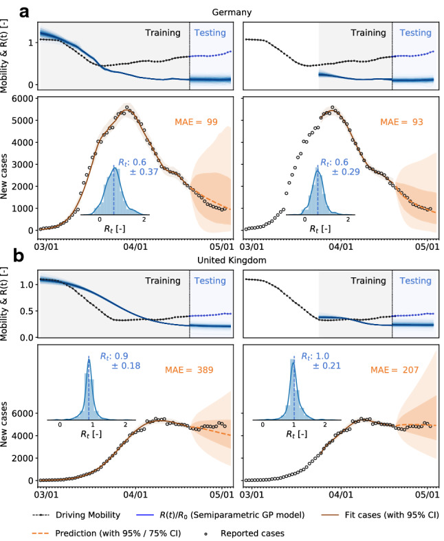
Local mobility, reproduction number, reported cases, and forecasting for Germany and the UK. Both models are trained on the full data set and on the data points after the mobility break down. Histograms show posterior distributions of last time step of predicted effective reproduction number R(t). Orange dashed curve indicates the 14-day forecast, and orange zones indicate the 95% and 75% confidence intervals and associated mean absolute errors
Fig. 10.

Local mobility, reproduction number, reported cases, and forecasting with different training sets. a Two-week forecast with training on the full available data set and b Two-week forecast with training on reduced data set beginning on April 1, 2020
Local mobility data can be used to identify possible super-spreading events. Super-spreading events are characterized by a local outbreak when a large population comes in close contact for a significant period of time. Examples include sporting events, parades, festivals, religious ceremonies, and carnivals. Unavoidably, these events are associated with large population movement that can be captured by mobility data. For instance, the Carnival season between February 20 and 26 in the Heinsberg district drew large crowds and it is believed to be the first COVID-19 hotspot in Germany (Streeck et al. 2020). Figure 6 shows the mobility data of the city of Cologne, approximately 70km from Heinsberg. The spike in mobility is directly followed by the epidemic outbreak and correlated with a change in the reproduction number with an adaptation time of 17 days. This highly localized event rippled across the entire country with an adaptation time of about 40 days.
Fig. 6.

Local mobility, reproduction number, and reported cases of a super-spreading event. a The Heinsberg Carnival took place between February 20 and 26 (shaded region) and is associated with a large spike in mobility data in the nearby city of Cologne. b It is correlated with a local increase in the reproduction number in Cologne, approximately 17 days delayed, and a national increase, approximately 40 days delayed. Cases are depicted as cumulative case numbers
Discussion
The objective of this study was to explore to which extent global and local mobility are correlated with the effective reproduction number, and, accordingly, with the local outbreak dynamics. Using passenger air travel, cell phone mobility data, and reported COVID-19 cases across Europe, we showed that mobility and reproduction are correlated during the early stages of the outbreak, but become decorrelated during later stages. Interestingly, our study identified five distinct phases of the outbreak across all European countries that implemented political counter measures.
Outbreak: During the early stages of the pandemic, global mobility modulates the initial outbreak pattern. Various studies have shown that, especially during the very early stages of an outbreak, there is a close correlation between mobility and spreading of an infectious disease. For instance, the early pattern of COVID-19 closely mimics passenger air travel (Linka et al. 2020). Global mobility is key to seed the disease in new locations before its local growth. Tight travel restrictions and border control in the USA and in the entire European Union mark the end of this phase in mid-March. In response, air travel within the European Union dropped by 95% within less than two weeks. Yet, it is becoming increasingly clear now that most travel restrictions were implemented too late to protect most countries from a local outbreak of COVID-19 (Chinazzi et al. 2020). While global mobility as in Fig. 7 can be an important modulator at very low or zero case numbers (Linka et al. 2020), our study suggests that a country-specific analysis based on local mobility alone as in Fig. 3 is probably sufficient to explain the major outbreak dynamics. In addition, the current study focuses only on mobility, while other factors, for example, self-adopted human behavioral changes, could show similar correlation patterns.
Phase I: Once a location is hit by the pandemic, exponential growth governs the local outbreak dynamics. After local seeding, the outbreak dynamics become decorrelated from global mobility. Instead, the local number of cases increases rapidly and the question of health care resources becomes the focal point in political decision making. At this point, without any additional measures, the outbreak would naturally peak and decay toward the endemic equilibrium (Hethcote 2000). The timing of the peak, its magnitude, and condition of herd immunity are determined by the basic reproduction number (Kwok et al. 2020). For COVID-19, the basic reproduction number is on the order of three to six (Flaxman et al. 2020), for which models would predict a peak of active cases from 21% to 39% of the population, occurring between days 46 and 23, and herd immunity after 67% to 86% of the population has become infected.
Phase II: Outbreak control modulates the effective reproduction number by reducing local mobility. To stop the period of exponential growth, political measures, including local lockdown and limit to gatherings, have been implemented in almost all European countries to limit contact between infectious and susceptible individuals. The rapid reduction of car traffic to within less than two weeks in early March is an indicator for a successful contact reduction. Strikingly, in most countries, this reduction emerged naturally, well ahead of political intervention, as a result of voluntary behavioral changes in the population, see Fig. 2a–d.
Phase III: Reduced mobility reduces the number of new cases and initiates a flattening of the curve. In the outbreak dynamics, reduced local mobility induces a reduction of the effective reproduction number and with it convergence to an enforced equilibrium state, a converged state under given constraints, long before herd immunity is achieved in the entire population. The speed and magnitude by which the reproduction number drops are a measure of the effectiveness of public health interventions (Bhouri et al. 2020; Linka et al. 2020). For example, in Austria, a country that is known for its strict response to the pandemic dropped from 4.0 to 1.1 in only 16 days; in Sweden, a country that implemented relatively lose public restrictions, it dropped from 2.0 to 1.1 in as much as 33 days. Figure 4d highlights the special role of Sweden, experiencing an early second wave, or rather not leaving the first wave at all. In the hypothetical case of complete lockdown, the number of new cases, and with it the effective reproduction number, would go to zero. However, Fig. 1c shows that even under the strict restrictions enforced in most European countries, the average duration from the point a country hit 100 cases until the reproduction number went down to one is days. As long as remains lower than one, the number of new cases continues to decrease, although gradually. A limitation of our study is its sensitivity with respect to the date of reporting, which can vary significantly between different countries. We illustrate the impact of drawing the data from two different days of reporting, the onset of symptoms and the reported test results, and show a significant resulting time shift for the example of Germany in Fig. 9.
Fig. 9.

Local mobility, reproduction number, and reported cases in Germany comparing data at day of symptom onset vs. day of reporting. The model learns the time-varying effective reproduction number for symptom onset (red curve) from the symptom onset cases (black boxes) and the simulated cases (orange curve) and the time-varying effective reproduction number for reporting (blue curve) from the reported cases (black circles) and the simulated cases (brown curve). Distributions of the adaptation time for symptom onset (blue) and reported data (green) and of difference between symptom onset and reported data (red)
Phase IV: The gradual exit from lockdown reveals the effect of social learning. Following a period of rigorous lockdown, most European governments have begun to slowly relax the strict measures to reduce movement and contacts. This relaxation is clearly reflected in the mobility data in Fig. 2 as a slow increase in local mobility. Strikingly, in early June, the local mobility index in Fig. 2d increases even beyond its initial value in early March, which could suggest a seasonal trend or, probably more likely, the effect that driving has now taken over from flying. Two important features are now becoming apparent: First, there is an asymmetry in the decrease and increase in the reproduction number before and after lockdown that can be attributed to social learning and soft political intervention including face masks, physical distancing, and no large gatherings. Second, variations in the reproduction number during the early phases are highly correlated with changes in local mobility, while later they are not. Our analysis with training and testing suggests that as long as the disease remains endemic, trends in local mobility allow us to forecast the outbreak dynamics for a two-week window. This correlation has potentially important consequences: Some proposed exit strategies suggest either periodic or on-demand lockdown once the number of new cases begins to rise again. The general objective of most outbreak control strategies is to keep the effective reproduction number either strictly below one or slightly above. The problem with this approach is that by the time a critical rise becomes observable, the inertia of the exponential dynamics is already difficult to control and long periods of lockdown would become necessary to regain control. Our study shows that mobility can serve as a barometer to adjust particular sectors of the economy, in real time, to manage future effective reproduction numbers. Similar to a barometer that can indicate short-term changes in the weather, mobility can indicate short-term changes in the reproduction number. However, proper management would still require some local interpretation of these indicators, since every individual government might attempt to optimize different parameters under different constraints. For example, once the mobility index reaches a certain level, a local government could decide to increase or decrease gathering sizes or opening hours. Importantly, in this approach, the forecast of the reproduction number, the correlation levels, and the window of correlation can be updated in real time as new data become available.
2nd Wave: Complete decorrelation between mobility and reproduction indicates the end of the first wave. In the case of COVID-19, during the early stages of exponential growth, almost all European countries experienced a strong reduction in local mobility. Around mid-March, numerous political measures were implemented in different stages, ranging from prohibiting gatherings to complete lockdown, with a restriction to essential business only. During this period, the virus spread across Europe at low level in a non-trivial way, see Figs. 3 and 4d. Throughout this time window, individual mobility had a massive potential to accelerate the outbreak and generate large effective reproduction numbers. This observation agrees well with the existence of a distinct time lag and associated strong correlations between mobility and reproduction among all European countries within the full dataset, see Fig. 4a. Due to behavioral changes after the first phase of the outbreak, our analysis suggests that the time lag increased from initially to days, before mobility and reproduction decorrelate. This is clearly visible in the cross-correlation for different time intervals of the dataset in Fig. 4a and b. The decorrelation begins after the infectious curve peaks at , and the dynamics of traffic and reproduction become increasingly independent as the effective reproduction approaches zero, while local mobility keeps increasing. In this range, the number of infectious individuals is too low to be amplified by human mobility. For example, for the case of Austria, which was among the first countries in Europe to aggressively implement outbreak control, we observe an early peak at the end of April in Fig. 4d. Austria was one of the first countries worldwide to report an effective reproduction number below one, which resulted in an early decorrelation and a vanishing distinct time shift between local mobility and reproduction, see Fig. 4a. The effect of decorrelation at low new case numbers is inherently built into our model: The latent variable formulation of the effective reproduction number R(t), as a function of local mobility within the SEIR model, becomes increasingly less sensitive to mobility changes for a low infectious population. This trend is robust and also holds for more complex compartment models including the SEIIRD model with an undetected population of asymptomatic individuals and a simultaneously fitted deceased population as we show in Fig. 8. Interestingly, the new increase in the effective reproduction number beyond one, , in response to the gradual exit marks a new increase in cases and the beginning of the second wave, that we can clearly see in Figs. 1 and 3 .
Fig. 8.

Local reported and simulated cases and deaths across Europe. a The hierarchical SEIIRD model learns the time-varying effective reproduction number R(t) from the reported cases (black circles) and deaths (blue circles) for varying adaptation times ; b adaptation time distribution indicates an adaptation time of days; c box plots of country-specific case fatality rates ; and d box plots of country-specific detection fractions
Taken together, the strong correlation between mobility and reproduction in the endemic phase, and the loss of correlation in the later phases, suggest that mobility is a reliable predictor of outbreak dynamics. Our study suggests that biweekly mobility trends can be used to stratify different phases of the pandemic, identify super-spreading events, and guide political decision making. Mobility is a suitable pandemic barometer.
Acknowledgements
This work was supported by a DAAD Fellowship to Kevin Linka, by the Engineering and Physical Sciences Research Council Grant EP/R020205/1 to Alain Goriely, and by a Stanford Bio-X IIP seed grant and the National Institutes of Health grant U01 HL119578 to Ellen Kuhl. This work was also undertaken, in part, as a contribution to the Rapid Assistance in Modelling the Pandemic RAMP initiative, coordinated by the Royal Society for which Alain Goriely is a task leader.
Appendix
Network modeling. Figure 7 shows results of the network model including both global and local mobility. The global mobility represents the air traffic data in each country, and the local mobility represents the driving mobility.
Prior selection. We constrain our models by an appropriate selection of model parameter prior distributions. We distinguish between a set of informative and uninformative priors. The set of informative priors contains the initial populations and , the basic reproduction number , the adaptation time and the transition time T. We model the initial infectious population and the initial exposed population by broad log-normal prior distributions. As median values, we select the number of new cases from the initial time point for the initial infectious population and the number of new cases from day three of our simulations for the initial exposed population to represent a latency period of . Since both, and , represent the total number of infectious and exposed individuals, their numbers cannot be directly inferred from case data alone and we model them both as unknown parameters. We assume a broad normal prior for the basic reproduction number with a median of 2, a normal prior for the adaptation time with a median of 14 days, and a log-normal prior of the transition time T with a median of 10 days (Linka et al. 2020), both with a fairly wide uncertainty on the priors. The set of flat-uninformative priors contains the priors of the Gaussian process model , , k, m, and , the travel coefficient , and the width of the likelihood function . For the priors of the Gaussian process model are the two kernel hyperparameters and to define the exponentiated quadratic form of the covariance function and the priors of the piecewise linear trend change in the mean function of the covariance function k, m, and . We select a flat normal prior for the travel coefficient and a scale factor of the width of the likelihood function as , which implies that the daily change in reported cases can be up to ten times larger than actually reported. Tables 1 and 2 summarize our priors for the SEIR and SEIIR models.
Local epidemiology modeling - SEIIRD model. To illustrate that our method is robust to disease parameters beyond the classical SEIR model, we expand the SEIR model for the local epidemiology of COVID-19 from Eq. (1) to an SEIIRD model with six compartments, the susceptible, exposed, detected infectious, hidden infectious, recovered, and deceased populations. These six compartments are governed by the following set of ordinary differential equations,
| A.1 |
The transition rates between the compartments, , , , and are inverses of the contact period , the latent period , the infectious period , and the survival period . The SEIIRD model splits the initial infectious group of the SEIR model in Eq. (1) into a detected group, , and a hidden undetected group, , where is the detection fraction and . From the detected group , individuals can transition into the recovered group R at a fraction or into the deceased group D at a fraction , where is the case fatality rate. We interpret the latent, infectious, and survival periods A, C, and K as disease-specific and static, and the contact period B(t) as behavior specific and dynamic. Using the dynamic contact period B(t), we calculate the effective reproduction number to quantify the outbreak dynamics.
Bayesian parameter inference. We need to estimate a set of 15 parameters including a set of eight parameters for the SEIIRD model, , and a set of seven parameters for the semi-parametric model, . As before, we fix the latency and infectious periods to days and days and estimate the remaining set of 13 model parameters using Bayesian inference with Markov Chain Monte Carlo sampling. In contrast to the SEIR model, we now fit two data sets simultaneously (Kergassner et al. 2020; Wang et al. 2020), the new daily detected cases, , and the daily new deaths, , which we extract as the differences between the today’s and yesterday’s confirmed cases and deaths (European Center for Disease Prevention and Control 2020) and smoothen using a seven-day moving average on the data. For both fits, we adopted a Student’s t distribution for the likelihood between the new daily reported data, and , and the model predictions, and , with new-case- and new-deaths-number-dependent widths (Dehning et al. 2020),
| A.2 |
where and represent the widths of the likelihoods and between the daily new reported cases and deaths and and the associated modeled new cases and deaths and . Again, we apply Bayes’ rule to obtain the posterior distributions of the parameters on the basis of the prior distributions specified in Table 2, and the reported cases and deaths themselves, which we infer approximately by employing the NO-U-Turn sampler (NUTS) (Hoffman and Gelman 2014) implementation of the Python package PyMC3 (Salvatier et al. 2016). Table 2 summarizes the priors on our SEIIRD model parameters.
Table 2.
Priors on SEIIRD model parameters
| Variable | Prior distribution | |
|---|---|---|
| Basic reproduction | Normal(2, 1.5) | |
| Standard deviation | HalfNormal(1.5) | |
| Adaptation time | Normal(14, 14) | |
| Standard deviation | HalfNormal(15) | |
| T | Transition time | LogNormal(, 0.8) |
| Standard deviation | HalfNormal(0.8) | |
| Hyperparameter | Gamma(2, 0.1) | |
| Hyperparameter | HalfCauchy(0.5) | |
| k | Growth rate | Normal(1, 1) |
| m | Offset | Normal(1, 1) |
| Rate adjustment | Normal(0, 2, shape=) | |
| K | Survival period | Normal(6.5,1) |
| Detection fraction | LogNormal(, 0.1) | |
| Case fatality rate | LogNormal(, 1.0) | |
| Initial detected inf | LogNormal(,1.0) | |
| Initial hidden inf | Deterministic() | |
| Initial exposed | LogNormal(,1.0) | |
| Likelihood width | HalfCauchy() | |
| Likelihood width | HalfCauchy() |
Reported and simulated cases and deaths. Figure 8 shows the reported and simulated cases and deaths across Europe. The hierarchical SEIIRD model learns the time-varying effective reproduction number R(t) from both the reported cases and deaths in Fig. 8 (a) for varying adaptation times . The learnt survival period is days. The adaptation time distribution in Fig. 8 (b) indicates an adaptation time of days. The box plots in Fig. 8 (c & d) show the country-specific case fatality rates and detection fractions . These results suggest that our method is not only applicable to the classical SEIR model but extends equally to more sophisticated models like the SEIIRD model with additional hidden and deceased compartments and can not only fit the reported case data, but also simultaneously reported cases and deaths.
Sensitivity with respect to date of reporting. In our main study, we interpret the daily reported case number from a central European data base (European Center for Disease Prevention and Control 2020) as the infectious population and fit this case number against the daily change of the infectious population of our SEIR model. Arguably, the “date of reporting” can mean different things for different countries, and it can vary hugely between infection, symptom onset, testing, positive confirmed, and reporting. This implies that our time delay between mobility and reproduction is highly sensitive to the local testing logistics.
Table 3 illustrates difference between symptom onset and reporting for four representative countries (European Center for Disease Prevention and Control 2020). For example, in Germany, the “date of reporting” represents the date at which a sample swab is sent to laboratory testing, although the actual date at which authorities are notified will be several days later. To illustrate the difference between symptom onset and reporting, we perform the same SEIR model analysis based on two different reported data sets , symptom onset data (Robert Koch Institute 2020b) and reporting data (European Center for Disease Prevention and Control 2020), which includes the data that we used throughout this study.
Table 3.
Time delay between symptoms and reporting
| Country | Median (days) | Mean (days) |
|---|---|---|
| EU/EEA and UK | 5 | 7 |
| Estonia | 5 | 6 |
| Luxembourg | 5 | 6 |
| Romania | 5 | 7 |
| UK | 4 | 4 |
Figure 9 illustrates the learned time-varying effective reproduction numbers for both symptom onset and reporting data, and the model fit of the simulated cases to the two data sets. The time shift in the two data sets results in a time shift of the model fit, and with it, a time shift in the effective reproduction number curves. The resulting adaptation time distributions vary between days for the system onset data and days for the reported data with a mean difference of 8.7 days. This study highlights the sensitivity of the data to the reporting logistics. Unfortunately, system onset data were not available for all countries in the European Union, and we can only show the sensitivity here, rather than using system onset data throughout our entire study, which would have been more unified and accurate.
Forecasting. Figure 10 compares the results of a two-week forecasting with different training sets for all ten European countries. Figure 10a uses the full available data set, whereas Fig. 10b uses only a reduced data set beginning on April 1, 2020, to train the model.
Footnotes
Publisher's Note
Springer Nature remains neutral with regard to jurisdictional claims in published maps and institutional affiliations.
Contributor Information
Kevin Linka, Email: klinka@stanford.edu.
Alain Goriely, Email: alain.goriely@maths.ox.ac.uk.
Ellen Kuhl, Email: ekuhl@stanford.edu.
References
- Ainslie KE, Walters CE, Fu H, Bhatia S, Wang H, Xi X, Baguelin M, Bhatt S, Boonyasiri A, Boyd O. and others. Evidence of initial success for China exiting COVID-19 social distancing policy after achieving containment. Wellcome Open Res 5:81 (2020) [DOI] [PMC free article] [PubMed]
- Aleta A, Martin-Corral D, Pastore y Piontti A, Ajelli M, Litvinova M, Chinazzi M, Dean NE, Halloran ME, Longini IM, Merler S, Pentland A, Vespignani A, Moro E, Moreno Y (2020) Modeling the impact of social distancing, testing, contact tracing and household quarantine on second-wave scenarios of the COVID-19 epidemic. medRxiv 10.1101/2020.05.06.20092841 [DOI] [PMC free article] [PubMed]
- Apple Mobility Trends (2020). https://www.apple.com/covid19/mobility. Accessed 2020-08-04
- Bhouri MA, Sahli Costabal F, Wang H, Linka K, Peirlinck M, Kuhl E, Perdikaris P (2020) COVID-19 dynamics across the US: A deep learning study of human mobility and social behavior. medRxiv 10.1101/2020.09.20.20198432
- Chinazzi M, Davis JT, Ajelli M, Gioannini C, Litvinova M, Merler S, Pastore Piontti A, Mu K, Rossi L, Sun K, Viboud C, Xiong X, Yu H, Halloran ME, Longini IM, Vespignani A. The effect of travel restrictions on the spread of the 2019 novel coronavirus (COVID-19) outbreak. Science. 2020;368:395–400. doi: 10.1126/science.aba9757. [DOI] [PMC free article] [PubMed] [Google Scholar]
- Dehning J, Zierenberg J, Spitzner FP, Wibral M, Neto JP, Wilczek M, Priesemann V. Inferring COVID-19 spreading rates and potential change points for case number forecasts. Science. 2020 doi: 10.1126/science.abb9789. [DOI] [PMC free article] [PubMed] [Google Scholar]
- Enserink M, Kupferschmidt K. With COVID-19, modeling takes on life and death importance. Science. 2020;367:1414–1415. doi: 10.1126/science.367.6485.1414-b. [DOI] [PubMed] [Google Scholar]
- Eurocontrol - Aviation Data (2020). https://ansperformance.eu/data/. Accessed 2020-08-04
- European Center for Disease Prevention and Control - Covid-19 surveillance report (2020).https://www.ecdc.europa.eu/covid19-surveillance-report.ecdc.europa.eu/#5_risk_groups_mostaffected. Accessed 2020-08-04
- European Center for Disease Prevention and Control-Covid-19 situation update worldwide (2020).https://www.ecdc.europa.eu/en/geographical-distribution-2019-ncov-cases. Accessed 2020-08-04
- Eurostat (2020). https://ec.europa.eu/eurostat. Accessed 2020-08-04
- Flaxman S, Mishra S, Gandy A, Unwin JT, Coupland H, Mellan TA, Zhu H, Berah T, Eaton JW, Guzman P, Schmit N, Callizo L, and Imperial College COVID-19 Response Team. Estimating the number of infections and the impact of non-pharmaceutical interventions on COVID-19 in European countries: technical description update (2020). arXiv:2004.11342
- Gao S, Rao J, Kang Y, Liang Y, Kruse J. Mapping county-level mobility pattern changes in the United States in response to COVID-19. SIGSPATIAL Special. 2020;12:16–26. doi: 10.1145/3404820.3404824. [DOI] [Google Scholar]
- Genton MG. Classes of kernels for machine learning: a statistics perspective. J Mach Learn Res. 2001;2:299–312. [Google Scholar]
- He X, Lau EH, Wu P, Deng X, Wang J, Hao X, Lau YC, Wong JY, Guan Y, Tan X, Mo X. Temporal dynamics in viral shedding and transmissibility of COVID-19. Nature Med. 2020;26:672–675. doi: 10.1038/s41591-020-0869-5. [DOI] [PubMed] [Google Scholar]
- Hethcote HW. The mathematics of infectious diseases. SIAM Rev. 2000;42:599–653. doi: 10.1137/S0036144500371907. [DOI] [Google Scholar]
- Hoffman MD, Gelman A. The No-U-Turn sampler: adaptively setting path lengths in Hamiltonian Monte Carlo. J Mach Learn Res. 2014;15(1):1593–1623. [Google Scholar]
- Hufnagel L, Brockmann D, Geisel T. Forecast and control of epidemics in a globalized world. Proc National Acad Sci. 2004;101:15124–15129. doi: 10.1073/pnas.0308344101. [DOI] [PMC free article] [PubMed] [Google Scholar]
- Kergassner A, Burkhardt C, Lippold D, Nistler S, Kergassner M, Steinmann P, Budday D, Budday S (2020) Meso-scale modeling of COVID-19 spatio-temporal outbreak dynamics in Germany. medRxiv (2020) 10.1101/2020.06.10.20126771. Computational Mechanics (2020), in press
- Kraemer MU, Yang C-H, Gutierrez B, Wu C-H, Klein B, Pigott D, du Plessis L, Faria NR, Li R, Hanage WP, Brownstein JS, Layan M, Vespignani A, Tian H, Dye C, Pybus OG, Scarpino SV. The effect of human mobility and control measures on the COVID-19 epidemic in China. Science. 2020;368:493–497. doi: 10.1126/science.abb4218. [DOI] [PMC free article] [PubMed] [Google Scholar]
- Kucharski A, Russel TW, Diamond C, Liu Y, Edmunds J, Funk S, Eggo RM, Sun F, Jit M, Munday JD. and others Early dynamics of transmission and control of COVID-19: a mathematical modelling study. Lancet Infectious Diseases. 2020 doi: 10.1016/S1473-3099(20)30144-4. [DOI] [PMC free article] [PubMed] [Google Scholar]
- Kuhl E. Data-driven modeling of COVID-19 - Lessons learned. Extreme Mech Lett. 2020;40:100921. doi: 10.1016/j.eml.2020.100921. [DOI] [PMC free article] [PubMed] [Google Scholar]
- Kwok K, Lai F, Wei W, Wong S, Tang JWT. Herd immunity-estimating the level required to halt the COVID-19 epidemics in affected countries. J Infection. 2020;80:e32–e33. doi: 10.1016/j.jinf.2020.03.027. [DOI] [PMC free article] [PubMed] [Google Scholar]
- Lange KL, Little RJA, Taylor MG. Robust statistical modeling using the t distribution. J Am Statist Assoc. 1989;84:881–896. [Google Scholar]
- Lauer SA, Grantz KH, Bi Q, Jones FK, Zheng Q, Meredith HR, Azman AS, Reich NG, Lessler J. The incubation period of coronavirus disease 2019 (COVID-19) from publicly reported confirmed cases: estimation and application. Ann Internal Med. 2020 doi: 10.7326/M20-0504. [DOI] [PMC free article] [PubMed] [Google Scholar]
- Lawrence N. Probabilistic non-linear principal component analysis with Gaussian process latent variable models. J Mach Learn Res. 2005;6:1783–1816. [Google Scholar]
- Li Q, Guan X, Wu P, Wang X, Zhou L, Tong Y, Ren R, Leung KSM, Lau EHY, Wong JY, Xing X, Xiang N, Wu Y, Li C, Chen Q, Li D, Liu T, Zhao J, Liu M, Tu W, Chen C, Jin L, Yang R, Wang Q, Zhou S, Wang R, Liu H, Luo Y, Liu Y, Shao G, Li H, Tao Z, Yang Y, Deng Z, Liu B, Ma Z, Zhang Y, Shi G, Lam TTY, Wu JT, Gao GF, Cowling BJ, Yang B, Leung GM, Feng Z. Early transmission dynamics in Wuhan, China, of novelcoronavirus-infected pneumonia. New Engl J Med. 2020;382:1199–1207. doi: 10.1056/NEJMoa2001316. [DOI] [PMC free article] [PubMed] [Google Scholar]
- Linka K, Peirlinck M, Sahli Costabal F, Kuhl E. Outbreak dynamics of COVID-19 in Europe and the effect of travel restrictions. Comput Methods Biomech Biomed Eng. 2020;23:710–717. doi: 10.1080/10255842.2020.1759560. [DOI] [PMC free article] [PubMed] [Google Scholar]
- Linka K, Rahman P, Goriely A, Kuhl E. Is it safe to lift COVID-19 travel restrictions? The Newfoundland story. Comput Mech. 2020;66:1081–1092. doi: 10.1007/s00466-020-01899-x. [DOI] [PMC free article] [PubMed] [Google Scholar]
- Linka K, Peirlinck M, Kuhl E. The reproduction number of COVID-19 and its correlation with public health interventions. Comput Mech. 2020;66:1035–1050. doi: 10.1007/s00466-020-01880-8. [DOI] [PMC free article] [PubMed] [Google Scholar]
- Maier BF, Brockmann D. Effective containment explains subexponential growth in recent confirmed COVID-19 cases in China. Science. 2020;368:742–746. doi: 10.1126/science.abb4557. [DOI] [PMC free article] [PubMed] [Google Scholar]
- Oliver N, Lepri B, Sterly H, Lambiotte R, Delataille S, De Nadai M, Letouzé E, Salah A, Benjamins R, Cattuto C, Colizza V, de Cordes N, Fraiberger S, Koebe T, Lehmann S, Murillo J, Pentland A, Pham P, Pivetta F, Saramäki J, Scarpino S, Tizzoni M, Verhulst Michele S, Vinck P. Mobile phone data for informing public health actions across the COVID-19 pandemic life cycle. Sci Adv. 2020 doi: 10.1126/sciadv.abc0764. [DOI] [PMC free article] [PubMed] [Google Scholar]
- Pan X, Cheng D, Xia Y, Wu X, Li T, Ou X, Zhou L, Liu J. Asymptomatic cases in a family cluster with SARS-CoV-2 infection. Lancet Infectious Diseases. 2020;20:410–411. doi: 10.1016/S1473-3099(20)30114-6. [DOI] [PMC free article] [PubMed] [Google Scholar]
- Parshani R, Carmi S, Havlin S. Epidemic threshold for the susceptible-infectious-susceptible model on random networks. Phys Rev Lett. 2010;104:258–701. doi: 10.1103/PhysRevLett.104.258701. [DOI] [PubMed] [Google Scholar]
- Peirlinck M, Linka K, Sahli Costabal F, Kuhl E. Outbreak dynamics of COVID-19 in China and the United States. Biomech Model Mechanobiol. 2020;19:2179–2193. doi: 10.1007/s10237-020-01332-5. [DOI] [PMC free article] [PubMed] [Google Scholar]
- Rasmussen CE (2003) Gaussian processes in machine learning. Summer School Mach Learn 63–71
- Robert Koch Institute (2020a) COVID-19 und Mobilität. https://rki.mobility-covid19.teralytics.net/. Accessed: 2020-08-04
- Robert Koch Institute (2020b) COVID-19-Dashboard. https://experience.arcgis.com/experience/. Accessed: 2020-08-04
- Salvatier J, Wiecki TV, Fonnesbeck C. Probabilistic programming in Python using PyMC3. Peer J Comput Sci. 2016;2:e55. doi: 10.7717/peerj-cs.55. [DOI] [Google Scholar]
- Streeck H, Schulte B, Kümmerer BM, Richter E, Höller T, Fuhrmann C, Bartok E, Dolscheid R, Berger M, Wessendorf L, Eschbach-Bludau M, Kellings A, Schwaiger A, Coenen M, Hoffmann P, Stoffel-Wagner B, Nöthen MM, Eis-Hübinger AM, Exner2 M, Schmithausen RM, Schmid M, Hartmann G (2020) Infection fatality rate of SARS-CoV-2 infection in a German community with a super-spreading event. medRxiv 10.1101/2020.05.04.20090076
- Taylor SJ, Letham B. Forecasting at scale. Am Statist. 2018;72:37–45. doi: 10.1080/00031305.2017.1380080. [DOI] [Google Scholar]
- Thompson RN. Epidemiological models are important tools for guiding COVID-19 interventions. BMC Med. 2020;104:152. doi: 10.1186/s12916-020-01628-4. [DOI] [PMC free article] [PubMed] [Google Scholar]
- Unwin H, Mishra S, Bradley V, Gandy A, Vollmer M, Mellan T, Coupland H, Ainslie K, Whittaker C, Ish-Horowicz J. and others. Report 23: State-level tracking of COVID-19 in the United States. Preprint (2020) 10.25561/79231 [DOI] [PMC free article] [PubMed]
- Wang Z, Zhang X, Teichert G, Carrasco-Teja M, Garikipati K (2020) System inference for the spatio-temporal evolution of infectious diseases: Michigan in the time of COVID-19. Computational Mechanics in press [DOI] [PMC free article] [PubMed]
- Wu JT, Leung K, Leung GM. Nowcasting and forecasting the potential domestic and international spread of the 2019-nCoV outbreak originating in Wuhan, China: a modelling study. The Lancet. 2020;395(10225):689–697. doi: 10.1016/S0140-6736(20)30260-9. [DOI] [PMC free article] [PubMed] [Google Scholar]
- Zhang J, Litvinova M, Liang Y, Wang Y, Wang W, Zhao S, Wu Q, Merler S, Viboud C, Vespignani A, Ajelli M, Yu H. Changes in contact patterns shape the dynamics of the COVID-19 outbreak in China. Science. 2020 doi: 10.1126/science.abb8001. [DOI] [PMC free article] [PubMed] [Google Scholar]