DEEP NEURAL NETWORK (DNN) FOR WATER/FAT SEPARATION: SUPERVISED TRAINING, UNSUPERVISED TRAINING, AND NO TRAINING

Abstract

Purpose:

To use a deep neural network (DNN) for solving the optimization problem of water/fat separation and to compare supervised and unsupervised training.

Methods:

The current T2*-IDEAL algorithm for solving water/fat separation is dependent on initialization. Recently, DNN has been proposed to solve water/fat separation without the need for suitable initialization. However, this approach requires supervised training of DNN (STD) using the reference water/fat separation images. Here we propose two novel DNN water/fat separation methods 1) unsupervised training of DNN (UTD) using the physical forward problem as the cost function during training, and 2) no-training of DNN (NTD) using physical cost and backpropagation to directly reconstruct a single dataset. The STD, UTD and NTD methods were compared with the reference T2*-IDEAL.

Results:

All DNN methods generated consistent water/fat separation results that agreed well with T2*-IDEAL under proper initialization.

Conclusion:

The water/fat separation problem can be solved using unsupervised deep neural networks.

INTRODUCTION

R2* corrected water/fat separation estimating water, fat and inhomogeneous field from gradient-recalled echo (GRE) signal is a necessary step in quantitative susceptibility mapping to remove the associated chemical shift contribution to the field (1-5). Several algorithms, including hierarchical multiresolution separation, multi-step adaptive fitting, and T2*-IDEAL, have been proposed to decompose the water/fat separation problem into linear (water and fat) and nonlinear (field and R2*) subproblems and solve these problems iteratively (6-8). Water/fat separation is a nonlinear nonconvex problem that requires a suitable initial guess to converge to a global minimum. Multiple solutions including 2D and 3D graph cuts and in-phase echo-based acquisition have been proposed to generate an initial guess (3,9-11). The performances of these methods is dependent on the assumptions inherent in these methods, including single species dominant voxels, field smoothness, or fixed echo spacing to generate a suitable initial guess and avoid water/fat swapping (12).

Recently, deep neural networks (DNN) have been used to perform water/fat separation using conventional supervised training of DNN with reference data (STD) (13,14). This STD water/fat separation method does not require an initial guess with the potential use of fewer echoes to shorten the scan time, or improve SNR with the same scan time, and lessen dependency on acquisition parameters compared to current standard approaches (13,14). However, the training of STD requires reference water/fat reconstructions (labels), which can be challenging to calculate as discussed above (15).

In this work, we investigate an unsupervised training of DNN (UTD) method that uses the physical forward problem in T2*-IDEAL as the cost function during conventional training without a need for reference water/fat reconstructions (no labels). We further investigate no-training DNN (NTD) method using a cost function similar to that in unsupervised to reconstruct water/fat images directly from a single dataset. We compare the results of the STD, UTD, and NTD methods with current T2*-IDEAL method.

METHODS

Water/Fat Separation T2*-IDEAL

Water/fat separation and field estimation is a nonconvex problem of modeling multi-echo complex GRE signal (S) in terms of water content (W), fat content (F), field (f) and $R_2^{\ast }$ decay per voxel (8):

$$(W,F,f,R_2^{\ast })=\underset{W,F,f,R_2^{\ast }}{argmin}{\sum }_{j=1}^N{\Vert S_j-e^{-R_2^{\ast }{t}_j}{e}^{-i2\pi f{t}_j}(W+F{e}^{-i2\pi v_F{t}_j})\Vert }_2^2,$$ [1]

where N refers to the number of echoes, S_j is the GRE signal S at echo time t_j with j = 1,…, N, and v_F is the fat chemical shift in a single-peak model. T2*-IDEAL solves Eq.1 by decomposing into linear (W, F) and nonlinear (f, $R_2^{\ast }$) subproblems. With an initial guess for f and $R_2^{\ast }$, the linear subproblem for W and F can be solved. With updated W, F, the nonlinear subproblem for f and $R_2^{\ast }$ is linearized through first order Taylor expansion and solved using Gauss-Newton optimization (8). These steps are repeated until convergence is achieved. In this study, initial guesses for the field f and $R_2^{\ast }$ decay were generated using in-phase echoes (3). The subsequent solutions to Eq. 1 resulted in the reference reconstructions Ψ_REF(S)={W, F, f, $R_2^{\ast }$}.

Supervised Training DNN (STD) Water/Fat Separation

In this work, we adapted the approaches in recent works (13,14) and making W, F, f, and $R_2^{\ast }$ the target output of the network. A U-net type network Ψ(Sⁱ; θ) with network weights θ is trained on M training pairs {Sⁱ, Ψ_REF(Sⁱ)}, where Sⁱ and Ψ_REF(Sⁱ) = {W, F, f, $R_2^{\ast }$}, are the input complex gradient echo signal and the corresponding reference T2*-IDEAL reconstruction (reference), respectively. The cost function is given by:

$$E_{STD}=\frac{1}{2}{\sum }_{i=1}^M{\Vert {\Psi }_{REF}(S^i)-\Psi (S^i;\theta )\Vert }_2^2.$$ [2]

Unsupervised Training DNN (UTD) Water/Fat Separation

In the proposed method, termed unsupervised, we seek to use deep learning framework to calculate W, F, f, and $R_2^{\ast }$ without access to reference reconstructions (labels). This is done by using the physical forward problem in Eq. 1 as the cost function during training. This cost function is given by:

$$\begin{gathered} E_{UTD}=\frac{1}{2}{\sum }_{i=1}^M{\sum }_{j=1}^N{\Vert S_j^i-{\tilde{S}}_j\left(\Psi (S^i;\theta )\right)\Vert }_2^2, \\ \text{with}{\tilde{S}}_j(\Psi )=e^{-R_2^{\ast }{t}_j}{e}^{-i2\pi f{t}_j}(W+F{e}^{-i2\pi v_F{t}_j})\text{for}\Psi =\{W,F,f,R_2^{\ast }\}. \end{gathered}$$ [3]

No-Training DNN (NTD) Water/Fat Separation

Recently, a single test data is used to update DNN weights in deep image prior (16) and fidelity imposed network edit (17). This inspires the idea that DNN weights θ* initialized randomly may be updated on a single gradient echo data set S to minimize the cost function in Eq.3 in a single data set S.

$$E_{NTD}=\frac{1}{2}{\sum }_{j=1}^N{\Vert S_j-{\tilde{S}}_j\left(\Psi (S_j;\theta )\right)\Vert }_2^2$$ [4]

The resulting network weights are specific to the data S, and the resulting output Ψ(S; θ*) can be taken as the water/fat separation reconstruction of S. In contrast to the above STD and UTD that involve conventional training data, no training is required here, the cost function is the same as that in the unsupervised training. Therefore, this method is referred to as no-training DNN (NTD).

Network Architecture

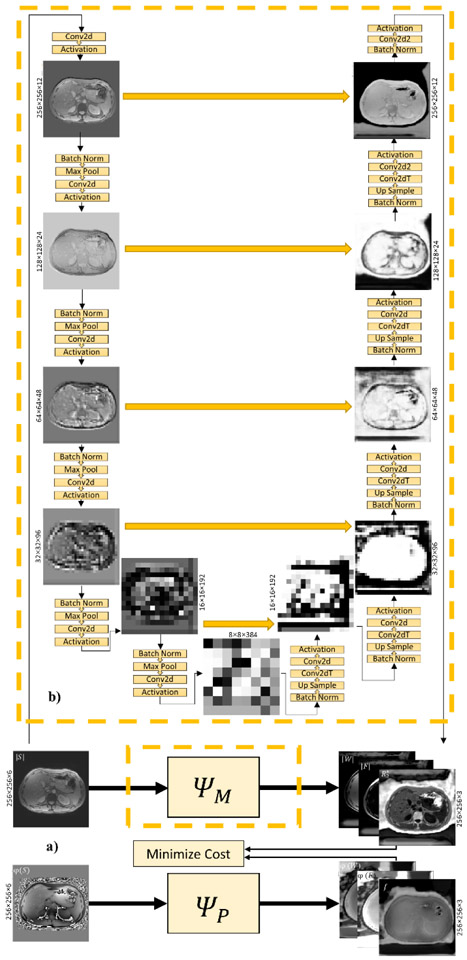
The network Ψ(Sⁱ; θ) consisted of two fully 2D convolutional neural sub-networks Ψ_M and Ψ_P with identical structure and encoding and decoding paths (Figure 1a):

$$\Psi (S;\theta )=\left[\begin{array}{c}\hfill {\Psi }_M(\mid S\mid ;{\theta }_M)\hfill \\ \hfill {\Psi }_P(\varphi (S);{\theta }_P)\hfill \end{array}\right]=\left[\begin{array}{c}\hfill \left[\begin{array}{c}\hfill \mid W\mid \hfill \\ \hfill \mid F\mid \hfill \\ \hfill R_2^{\ast }\hfill \end{array}\right]\hfill \\ \hfill \left[\begin{array}{c}\hfill \varphi (W)\hfill \\ \hfill \varphi (F)\hfill \\ \hfill f\hfill \end{array}\right]\hfill \end{array}\right]$$ [5]

Figure 1.

(a) The deep convolutional network used in this study consists of two sub-networks Ψ_M(∣S∣; θ_M) and Ψ_P(ϕ(S); θ_P) that have identical structure. The inputs of the sub-networks are the magnitude of the complex gradient echo images (∣S∣) and phase images (φ(S)), respectively. The outputs are the magnitude related components (magnitude of water ∣W∣ and fat ∣F∣, and R2*) and the phase related components (phase of water φ(W) and fat φ(F), and field f), respectively. (b) Depiction of the sub-network illustrating the output of intermediate layers.

Here, ∣S∣ and ϕ(S) are the magnitude and the phase of the complex GRE signal S, respectively, each containing N channels, one for each echo, ∣W∣ and ϕ(W) are the magnitude and the phase of the water map. ∣F∣ and ϕ(F) are the magnitude and the phase of the fat map. $\theta =\left[\begin{array}{c}\hfill {\theta }_M\hfill \\ \hfill {\theta }_P\hfill \end{array}\right]$ with θ_M and θ_P the network weights for the two sub-networks. The encoding paths included repeated blocks (n=5) each consisted of convolution (2×2), activation function (Sigmoid), batch normalization and max pooling (2×2). The decoding paths with repeated blocks (n=5) had similar architecture to the encoding path except max pooling was replaced with deconvolution and upsampling along with concatenation of corresponding feature maps with the encoding path [4]. The last block consists of convolution with linear activation function. Figure 1b shows the sub-networks Ψ_M architecture, representative input and output images for a test set in UTD method, along with outputs of intermediate layers. These show how learned features at different levels transform the input data into the final output images. Yellow arrows indicate concatenation of encoder and decoder layer outputs with the same feature maps. Training was performed using the ADAM optimizer (18).

Data Acquisition

Data was acquired in healthy volunteers (n=12) and patients (n=19), including thalassemia major (n=11), polycystic kidney disease (n=7), and suspected iron overload (n=1). Two 1.5T GE scanners (Signa HDxt, GE Healthcare, Waukesha, WI) with 8-channel cardiac coil were used to acquire data. The healthy subjects were imaged on both scanners using identical protocols (24 scans). Patients were scanned on one scanner, selected at random, using the same protocol (19 scans). This protocol contained a multi-echo 3D GRE sequence with the following imaging parameters: number of echoes = 6, unipolar readout gradients, flip angle = 5°, ΔTE = 2.3 msec, TR = 14.6 msec, acquired voxel size = 1.56×1.56×5 mm³, BW = 488 Hz/pixel, reconstruction matrix = 256×256×(28-36), ASSET acceleration factor = 1.25, and acquisition time of 20-27 sec.

Additional data was acquired for one experiment in 6 subjects (3 healthy volunteers, 3 iron-overload patients) scanned once at 1.5T Siemens scanner (Magnetom Aera, Siemens Healthcare, Erlangen, Germany) with an 18-channel body coil. The GRE imaging parameters for these 6 subjects were: number of echoes = 6, unipolar readout gradients, flip angle = 5°, TE₁ = 1.7 msec, ΔTE = 2.3 msec, TR = 15 msec, acquired voxel size = 2.2×1.56×8 mm³, BW = 1500 Hz/pixel, acquisition matrix = 256×192×(28-36), slice and phase Fourier encoding = 7/8, GRAPPA acceleration factor = 2 and acquisition time of 20-25 sec.

The study was approved by the Institutional Review Board and written informed consent was obtained from each participant.

Experiments and Quantitative Analysis

Multiple experiments were performed to assess the performance of DNN in water/fat separation and how supervised (STD), unsupervised (UTD), and no-training (NTD) compare against the T2*-IDEAL reference method. The network architecture for Ψ(S; θ) was identical between the three DNN methods. Parameters in STD and UTD include, number of epochs 2000, batch size 2, learning rate 0.001 for STD and 0.0006 for UTD. The learning rates were experimentally found to produce optimal results. In NTD, parameters include, number of epochs 10000, batch size 2, and learning rate 0.0006.

Experiment 1

To compare the supervised (STD), unsupervised (UTD), and no-training (NTD) methods with the reference T2*-IDEAL, training was performed on the combined sets of healthy subjects (2 scans each) and patients. This complex data of n=43 scans (256×256×1582×6) was split at subject level into testing (two subjects, 256×256×60×6, number of slices (60) vary depending on the selected subject) and training (256×256×1522×6). Next, in the healthy subject selected for testing, the corresponding images from the same subject (256×256×30×6) at the other scanner were removed from the training data. The remaining training data, randomly shuffled in slice direction, was further split (80%-20%) into training (256×256×1193×6) and the rest for validation (256x×256×299×6). The weights corresponding to the lowest validation loss during training was selected as the optimal weights to be used during testing. Training time in each epoch was ~80 seconds. The testing data comprised of a pair of subjects (one healthy volunteer, one patient). ROIs were drawn on the reference T2*-IDEAL water and proton density fat fraction maps $PDFF=\frac{\mid F\mid }{\mid F\mid +\mid W\mid }$, (to select regions with moderate and high fat content). Several ROIs were drawn including liver, adipose and visceral fat, aorta, spleen, kidney, vertebrae. The ROIs were copied on DNN images and measurements for each DNN method were compared with those on the reference T2*-IDEAL maps using correlation and Bland-Altman analysis. This experiment was repeated three times and at each time one pair of subjects (one healthy subject, one patient) were randomly selected and the rest of data was used for training/validation as discussed earlier. An additional experiment was carried out in the first pair of subjects, where the input format of the complex data was changed from magnitude/phase to real/imaginary to compare performance of STD, UTD, and NTD methods.

Experiment 2

This experiment tested the generalizability of the DNN methods and their dependence on acquisition parameters. For STD and UTD, n=43 scans (1.5T GE) were used for training and n=6 scans (1.5T Siemens) were used for testing. NTD was performed in these 6 (1.5T Siemens) subjects as well. The same ROI analysis as in the first experiment was carried out. Results from the 6 subjects were compared with the reference T2*-IDEAL images using correlation and Bland-Altman analysis.

Experiment 3

This experiment was designed to test the robustness of the NTD method. NTD, which required not training, was performed in all n=43 scans. The same ROI analysis as in the first experiment was carried out. Results from these subjects were compared with the reference T2*-IDEAL output using correlation and Bland-Altman analysis. In one subject, NTD method results per epoch was compared with the T2*-IDEAL cost function per iteration when field was initialized with in-phase echoes (3) and conventional 2D graph cut method from ISMRM Fat-Water Toolbox (9,19).

For all experiments, the T2*-IDEAL reference reconstruction was performed on CPU (Intel, i7-5820k, 3.3 GHz, 64 GB,) using MATLAB (R2019a, MathWorks, Natick, MA) and all DNN algorithms were developed using Keras (2.2.4)/TensorFlow (R1.13) and trainings were performed on GPU (NVIDIA, Titan XP GP102, 1405 MHz, 12 GB).

RESULTS

Experiment 1

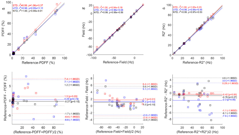
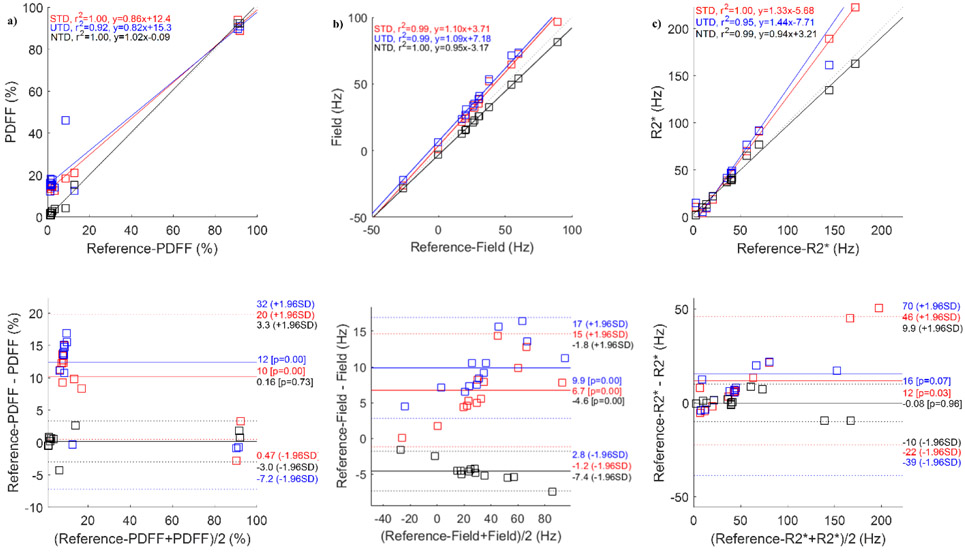
Figure 2 compares the network output results in one healthy subject. Shown are the reference T2*-IDEAL (Figure 2a), STD (Figure 2b), UTD (Figure 2c), and NTD (Figure 2d) reconstructions. While there is very good qualitative agreement among all methods, an artifact (yellow arrow) seen in the fat in the reference T2*-IDEAL and STD methods, has been removed in UTD and NTD methods. The correlation and Bland-Altman analysis in Figure 3 comparing PDFF (Figure 3a), field (Figure 3b) and R2* (Figure 3c) with the reference show excellent agreement. Corresponding test results for healthy volunteers in the 2^nd and 3^rd pair are shown in Figs. S2 and S4. Among the 3 subjects (Figs. 2, 3, S2, and S4) and all three methods, correlation analysis (average slope = 0.98, average R² = 0.99 over all parameters and Bland-Altman analysis (average mean difference, average +1.96SD, average −1.96SD) in PDFF (3.19, 0.26, −2.68) in %, field (3.93, 0.52, −2.85) in Hz, and R2* (2.39, −0.62, −3.65) in Hz showed very good agreement between DNN and the reference T2*-IDEAL. Supplementary Figure S1 shows the corresponding result when, instead of magnitude and phase, the real and imaginary components of the GRE signal are use as input for the network. While in this case water and fat images agree well with reference, field and R2* shows poor qualitative (Figure S1b-d) and quantitative (Figure S1e-g) agreement with the reference. This suggests while both formats (real/imaginary or magnitude/phase) have identical information content, spatial and temporal distribution of information differs from one format to another which makes the learning task easier in the latter case for the given network architecture.

Figure 2.

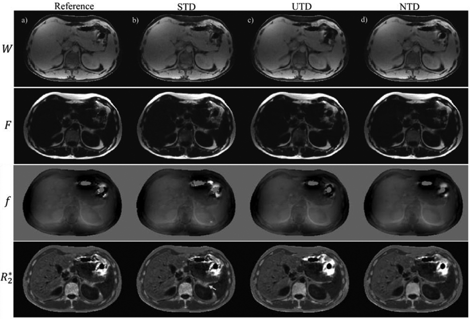
Water, fat, field and R2* reference images are shown (a) in a healthy volunteer. (b), (c), and (d) show corresponding results for supervised (STD), unsupervised (UTD), and no-training (NTD) methods. An artifact (yellow arrow) seen in STD and reference results is removed in UTD and NTD methods.

Figure 3.

ROI measurement correlation and Bland-Altman analysis comparing proton density fat fraction (a), field (b) and R2* (c) reference images with the corresponding results for supervised (STD), unsupervised (UTD), and no-training (NTD) methods in a healthy volunteer. Corresponding images are shown in Figure 2.

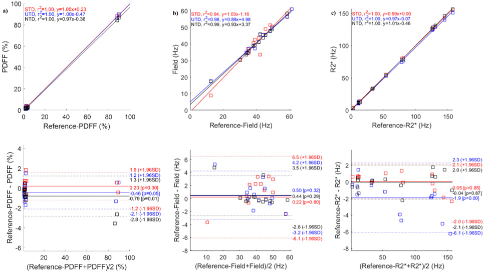
Figure 4 compares the DNN results in one patient with moderate iron-overload. Shown are the reference T2*-IDEAL (Figure 4a), STD (Figure 4b), UTD (Figure 4c), and NTD (Figure 4d) reconstructions. Very good qualitative agreement in both contrast and details is observed among these outputs. Correlation and Bland-Altman analysis in Figure 5 comparing PDFF (Figure 5a), field (Figure 5b) and R2* (Figure 5c) with the reference show good agreement. The results for another patient with iron overload and for a patient with polycystic kidney disease are shown in Figures S3 and S5. Among the 3 subjects (Figs. 3, 4, S3, and S5) and all three methods , correlation analysis (average slope = 0.98, average R² = 0.99) over all parameters and Bland-Altman analysis (average mean difference, average +1.96SD, average −1.96SD) in PDFF (2.1, −0.63, −3.34) in %, field (5.94, 0.68, −4.63) in Hz, and R2* (4.06, −0.19, −4.49) in Hz showed very good agreement between DNN and the reference T2*-IDEAL.

Figure 4.

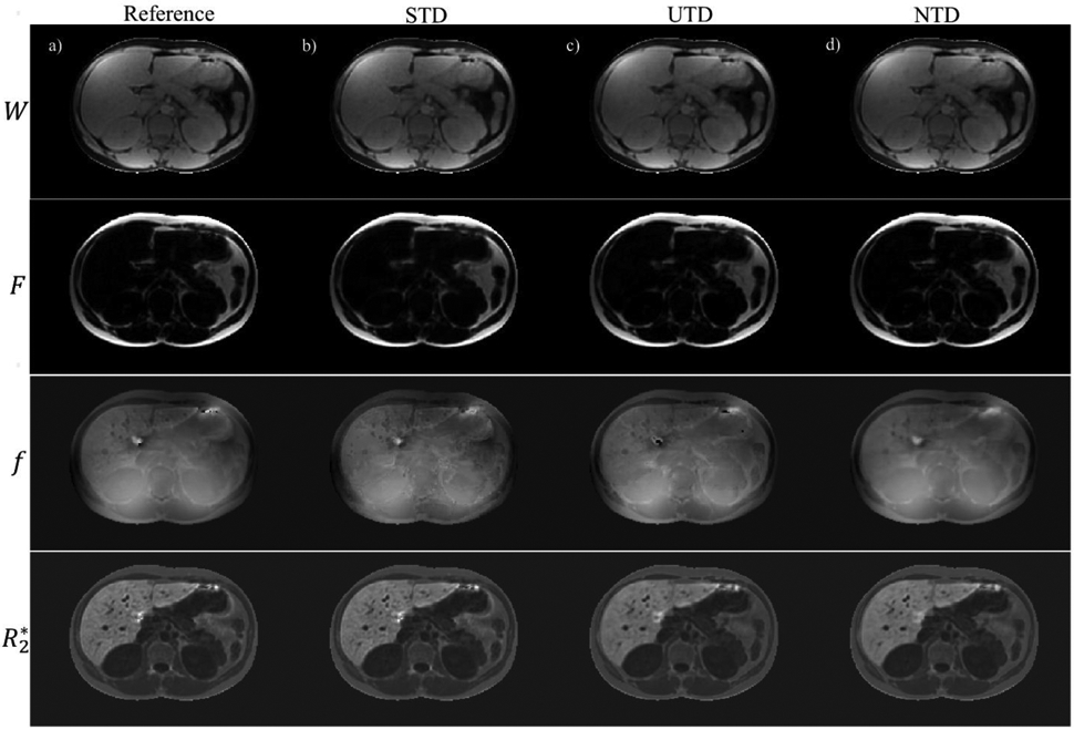
Water, fat, field and R2* reference images are shown (a) in an iron-overload patient. (b), (c), and (d) show corresponding results for supervised (STD), unsupervised (UTD), and no-training (NTD) methods. An artifact (yellow arrow) seen in STD and reference results is removed in UTD and NTD methods.

Figure 5.

ROI measurement correlation and Bland-Altman analysis comparing proton density fat fraction (a), field (b) and R2* (c) reference images with the corresponding results for supervised (STD), unsupervised (UTD), and no-training (NTD) methods in an iron-overload patient. Corresponding images are shown in Figure 4.

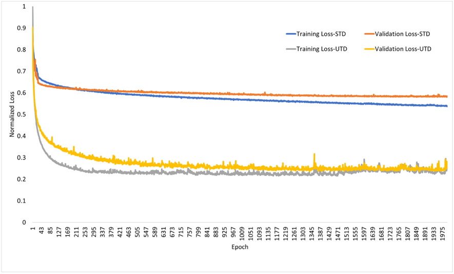
Figure 6 shows the normalized (with respect to epoch=1 training loss) training and validations losses for the STD and UTD methods. While validation loss for the STD method is initially (epoch < 250) lower than the training loss it becomes larger at later epochs. The validation loss remains consistently larger than the training loss for UTD. The total training time for both methods was similar (~40 hrs each).

Figure 6.

Normalized training and validation loss results for supervised (STD) and unsupervised (UTD) training methods.

Experiment 2

Figure 7 compares the DNN output for a healthy subject. Shown are the T2*-IDEAL (Figure 7a), STD (Figure 7b), UTD (Figure 7c), and NTD (Figure 7d) reconstructions. Very good qualitative and quantitative agreement between NTD and the reference T2*-IDEAL images are seen. In UTD and STD methods, while anatomical details agree well with the reference T2*-IDEAL, there is a lower agreement in contrast partially due to difference in acquisitions parameters including echo times between the training (GE, 1.5T) and testing (Siemens, 1.5T). The correlation and Bland-Altman plots in Figure 8 comparing reference T2*-IDEAL with NTD, in PDFF (Figure 8a), field (Figure 8b) and R2* (Figure 8c) show very good agreement between the two and moderate agreement in STD and UTD methods. Figure S6 shows ROI analysis correlation and Bland-Altman plots from all 6 subjects combined in PDFF (Fig S6a), field (Fig. S6b) and R2* (Fig S6c). NTD shows very good agreement, while there is moderate agreement in UTD and STD. This experiment shows NTD is generalizable while STD and UTD underperform due to difference in scanner and acquisition parameters between testing and training data.

Figure 7.

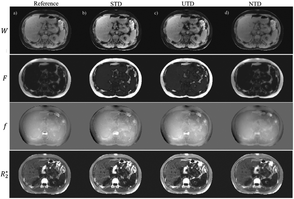
Water, fat, field and R2* reference images are shown (a) in a healthy subject. (b), (c), and (d) show corresponding results for supervised (STD), unsupervised (UTD), and no-training (NTD) methods when training (GE, 1.5T) and testing (Siemens, 1.5T) scanner and acquisition parameters were different.

Figure 8.

ROI measurement correlation and Bland-Altman analysis comparing proton density fat fraction (a), field (b) and R2* (c) reference images with the corresponding results for supervised (STD), unsupervised (UTD), and no-training (NTD) methods in a healthy subject when training (GE, 1.5T) and testing (Siemens, 1.5T) scanner and acquisition parameters were different. Corresponding images are shown in Figure 7.

Experiment 3

Figure 9 shows the ROI based correlation and Bland-Altman analysis in all 43 scans comparing NTD with T2*-IDEAL in PDFF (shown in Figure 9A), field (Figure 9B) and R2* (Figure 9C) demonstrating excellent agreement. Average slope and average R² were 0.99 over all parameters. Bland-Altman analysis (average mean difference, average +1.96SD, average −1.96SD) in PDFF (−0.72, 1.5, −2.9) in %, field (0.61, 4.8, −3.5) in Hz, and R2* (−1.3, 4.8, −7.4) in Hz showed very good agreement between NTD and the reference T2*-IDEAL.

Figure 9.

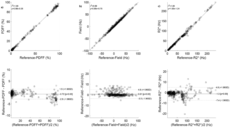
ROI measurement correlation and Bland-Altman analysis comparing no-training (NTD) method with the reference T2*-IDEAL for proton density fat fraction (a), field (b), and R2* (c) in 31 subjects (12 healthy volunteers, 19 patients).

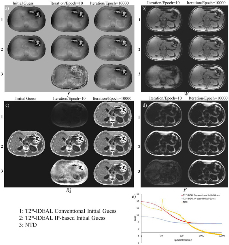
Figure 10 shows a comparison of NTD with T2*-IDEAL in a healthy volunteer. The T2*-IDEAL cost function per iteration is shown in the same graph as the NTD reconstruction cost per epoch. In the first row, T2*-IDEAL results of field (Figure 10a), water (Figure 10b), R2* (Figure 10c) and fat (Figure 10d) shows the results when field was initialized with conventional 2Dgraph cut method from ISMRM Fat-Water Toolbox (9,19). In the second row, the corresponding images show the result when IP-based initialization was used (the field and R2* obtained from the in-phase echoes in this case). The third row shows the proposed NTD results. The generated maps when using 10000 epochs are close the successful T2*-IDEAL result (1^st and 2^nd row) without a need for an initial guess. The corresponding T2*-IDEAL costs and NTD reconstruction loss are shown in Figure 10e. With conventional and IP-based field initialization, T2*-IDEAL requires ~100 iterations to converge. The proposed NTD method requires 10000 epochs for convergence. Computation time for each iteration and each epoch was similar (~1.3 seconds).

Figure 10.

Water/fat separation results comparing current T2*-IDEAL with conventional initialization (1) and IP-based (2) initialization, with the proposed NTD method (3) results for field (a), water (b), R2* (c), and fat (d). No initial guess was used for water and fat maps. Corresponding loss curves (e) are shown for T2*-IDEAL Vs. iteration and NTD Vs. epoch.

DISCUSSION AND CONCLUSION

Our results demonstrate the feasibility of an unsupervised deep neural network (DNN) framework both with training and without training to solve the water/fat separation problem. The proposed unsupervised training DNN (UTD) method does not require reference images as in supervised training DNN (STD), allowing the use of DNNs for training data that are unlabeled but for which physical model is known. The no-training DNN (NTD) method further allows using DNN reconstruction of a single data set (subject) for which a physical model is known.

For the nonlinear nonconvex water/fat separation problem, the reference T2*-IDEAL method uses traditional gradient descent optimization and is dependent on the initial guess. This problem may be alleviated using deep learning, as long as the labeled training data is sufficiently large to capture test data characteristics. Labeled data may be difficult to obtain as in water/fat separation problems. Unlabeled data are easier to obtain, but still it is difficult to ensure that training data do not lack test data characteristics. Accordingly, reconstruction directly from a test data without training is desirable, as in the reference T2*-IDEAL but without its dependence on initialization. This can be achieved using the proposed NTD.

The NTD method can overcome the initialization-dependence in traditional gradient descent based nonconvex optimization begs some intuitive explanation or interpretation, though rigorous explanation is currently not available. The cost function in DNN is minimized by adjusting network weights through backpropagation, which is achieved through iterative stochastic gradient descent (SGD). Perhaps SGD along with nonlinear functions in the network allows escaping local traps encountered in traditional gradient descent and the intensive computation in updating network weights facilitates some exhaustive search for a consistent minimum. The network weights updating on a single test data may converge as demonstrated in fidelity imposed network edit (17) and in deep image prior (16,20). Our data suggests that NTD can converge to a consistent minimum without initialization-dependence for the nonlinear nonconvex water/fat separation problem.

While some image details in STD, UTD, and NTD methods were different from the reference images, quantitative measurements in the liver include ROI measurements of several voxels and regions which is less dependent on image details (21,22). Our results showed while STD and UTD methods fail when acquisition parameters in training and testing data are different, NTD method is free from this limitation and can be generalized. The network architecture can be further optimized for this problem. For instance, we found changing activation function (Relu to Sigmoid) significantly improved field and R2* results in unsupervised training while not much change was observed in water and fat maps. Since field and R2* have a nonlinear relationship with respect to input complex signal while that of water and fat is linear, designing task-specific networks for Ψ_M(∣S∣; θ_M) and Ψ_P(ϕ(S); θ_P) may yield further improvement and potentially decrease the number of learned weights.

This study has a number of limitations. While the input data is complex, the networks only accept real values and two separate input channels were used instead. This potentially can change the noise properties and suboptimal network performance which can be addressed by including complex networks for this purpose (23). Generation of reference images requires solving the T2*-IDEAL problem which can be challenging to calculate depending on acquisition protocol. The advantage of the proposed unsupervised methods is they only require complex input signal for training. While the NTD method requires a large number of epochs to converge which is computationally expensive, one could use a previously trained network (trained on data with the same imaging parameters) and update the weights for the new data set (17). Only two scanner manufacturers and models were used for this study and variety in manufacturer, model and field strengths will help to further generalize. There were limited number of cases used for training in STD and UTD methods in this study and including more cases will strengthen network performance and reliability.

In summary, we demonstrated the feasibility of using unsupervised DNN to solve the water/fat problem with very good agreement compared to reference images.

DATA AVAILABILITY STATEMENT

The code and data that support the findings of this study are openly available in DL-MRI-Water-Fat-Separation at https://github.com/RaminJafari/DL-MRI-Water-Fat-Separation.

REFERENCES:

- 1.Reeder SB, Hu HH, Sirlin CB. Proton density fat-fraction: A standardized mr-based biomarker of tissue fat concentration. Journal of Magnetic Resonance Imaging 2012;36(5):1011–1014. [DOI] [PMC free article] [PubMed] [Google Scholar]
- 2.Labranche R, Gilbert G, Cerny M, Vu KN, Soulières D, Olivié D, Billiard JS, Yokoo T, Tang A. Liver Iron Quantification with MR Imaging: A Primer for Radiologists. Radiographics 2018;38(2):392–412. [DOI] [PubMed] [Google Scholar]
- 3.Jafari R, Sheth S, Spincemaille P, Nguyen TD, Prince MR, Wen Y, Guo Y, Deh K, Liu Z, Margolis D, Brittenham GM, Kierans AS, Wang Y. Rapid automated liver quantitative susceptibility mapping. J Magn Reson Imaging 2019;50(3):725–732. [DOI] [PMC free article] [PubMed] [Google Scholar]
- 4.Sharma SD, Hernando D, Horng DE, Reeder SB. Quantitative susceptibility mapping in the abdomen as an imaging biomarker of hepatic iron overload. Magn Reson Med 2015;74(3):673–683. [DOI] [PMC free article] [PubMed] [Google Scholar]
- 5.Guo Y, Liu Z, Wen Y, Spincemaille P, Zhang H, Jafari R, Zhang S, Eskreis-Winkler S, Gillen KM, Yi P, Feng Q, Feng Y, Wang Y. Quantitative susceptibility mapping of the spine using in-phase echoes to initialize inhomogeneous field and R2* for the nonconvex optimization problem of fat-water separation. NMR in Biomedicine 2019;32(11):e4156. [DOI] [PubMed] [Google Scholar]
- 6.Tsao J, Jiang Y. Hierarchical IDEAL: Fast, robust, and multiresolution separation of multiple chemical species from multiple echo times. Magnetic Resonance in Medicine 2013;70(1):155–159. [DOI] [PubMed] [Google Scholar]
- 7.Zhong X, Nickel MD, Kannengiesser SAR, Dale BM, Kiefer B, Bashir MR. Liver fat quantification using a multi-step adaptive fitting approach with multi-echo GRE imaging. Magnetic Resonance in Medicine 2014;72(5):1353–1365. [DOI] [PubMed] [Google Scholar]
- 8.Yu H, McKenzie CA, Shimakawa A, Vu AT, Brau AC, Beatty PJ, Pineda AR, Brittain JH, Reeder SB. Multiecho reconstruction for simultaneous water-fat decomposition and T2* estimation. J Magn Reson Imaging 2007;26(4):1153–1161. [DOI] [PubMed] [Google Scholar]
- 9.Hernando D, Kellman P, Haldar JP, Liang ZP. Robust water/fat separation in the presence of large field inhomogeneities using a graph cut algorithm. Magn Reson Med 2010;63(1):79–90. [DOI] [PMC free article] [PubMed] [Google Scholar]
- 10.Dong J, Liu T, Chen F, Zhou D, Dimov A, Raj A, Cheng Q, Spincemaille P, Wang Y. Simultaneous phase unwrapping and removal of chemical shift (SPURS) using graph cuts: application in quantitative susceptibility mapping. IEEE Trans Med Imaging 2015;34(2):531–540. [DOI] [PubMed] [Google Scholar]
- 11.Reeder SB, Wen Z, Yu H, Pineda AR, Gold GE, Markl M, Pelc NJ. Multicoil Dixon chemical species separation with an iterative least-squares estimation method. Magnetic Resonance in Medicine 2004;51(1):35–45. [DOI] [PubMed] [Google Scholar]
- 12.Sharma SD, Artz NS, Hernando D, Horng DE, Reeder SB. Improving chemical shift encoded water–fat separation using object-based information of the magnetic field inhomogeneity. Magnetic Resonance in Medicine 2015;73(2):597–604. [DOI] [PMC free article] [PubMed] [Google Scholar]
- 13.Goldfarb JW, Craft J, Cao JJ. Water–fat separation and parameter mapping in cardiac MRI via deep learning with a convolutional neural network. Journal of Magnetic Resonance Imaging 2019;50(2):655–665. [DOI] [PubMed] [Google Scholar]
- 14.Andersson J, Ahlström H, Kullberg J. Separation of water and fat signal in whole-body gradient echo scans using convolutional neural networks. Magnetic Resonance in Medicine 2019;82(3):1177–1186. [DOI] [PMC free article] [PubMed] [Google Scholar]
- 15.Yuji R, Geon H, Steven W. A Survey on Data Collection for Machine Learning: A Big Data - AI Integration Perspective. IEEE Transactions on Knowledge and Data Engineering 2019;PP:1–1. [Google Scholar]
- 16.Ulyanov D, Vedaldi A, Lempitsky V. Deep image prior. arXiv preprint arXiv:171110925 2017.
- 17.Zhang J, Liu Z, Zhang S, Zhang H, Spincemaille P, Nguyen TD, Sabuncu MR, Wang Y. Fidelity imposed network edit (FINE) for solving ill-posed image reconstruction. Neuroimage 2020;211:116579. [DOI] [PMC free article] [PubMed] [Google Scholar]
- 18.Kingma D, Ba J. Adam: A Method for Stochastic Optimization. 2014.
- 19.Hu HH, Börnert P, Hernando D, Kellman P, Ma J, Reeder S, Sirlin C. ISMRM workshop on fat-water separation: insights, applications and progress in MRI. Magn Reson Med 2012;68(2):378–388. [DOI] [PMC free article] [PubMed] [Google Scholar]
- 20.Jin KH, Gupta H, Yerly J, Stuber M, Unser M. Time-Dependent Deep Image Prior for Dynamic MRI. ArXiv 2019;abs/1910.01684. [DOI] [PubMed]
- 21.Wood JC, Enriquez C, Ghugre N, Tyzka JM, Carson S, Nelson MD, Coates TD. MRI R2 and R2* mapping accurately estimates hepatic iron concentration in transfusion-dependent thalassemia and sickle cell disease patients. Blood 2005;106(4):1460–1465. [DOI] [PMC free article] [PubMed] [Google Scholar]
- 22.Yokoo T, Serai SD, Pirasteh A, Bashir MR, Hamilton G, Hernando D, Hu HH, Hetterich H, Kühn J-P, Kukuk GM, Loomba R, Middleton MS, Obuchowski NA, Song JS, Tang A, Wu X, Reeder SB, Sirlin CB, Committee FtR-QPB. Linearity, Bias, and Precision of Hepatic Proton Density Fat Fraction Measurements by Using MR Imaging: A Meta-Analysis. Radiology 2018;286(2):486–498. [DOI] [PMC free article] [PubMed] [Google Scholar]
- 23.Virtue P, Yu S, Lustig M. BETTER THAN REAL: COMPLEX-VALUED NEURAL NETS FOR MRI FINGERPRINTING. 2017 24th Ieee International Conference on Image Processing (Icip) 2017:3953–3957. [Google Scholar]
Associated Data
This section collects any data citations, data availability statements, or supplementary materials included in this article.
Supplementary Materials