COVID-19 Diagnosis via DenseNet and Optimization of Transfer Learning Setting

Abstract

COVID-19 is an ongoing pandemic disease. To make more accurate diagnosis on COVID-19 than existing approaches, this paper proposed a novel method combining DenseNet and optimization of transfer learning setting (OTLS) strategy. Preprocessing was used to enhance, crop, and resize the collected chest CT images. Data augmentation method was used to increase the size of training set. A composite learning factor (CLF) was employed which assigned different learning factor to three types of layers: frozen layers, middle layers, and new layers. Meanwhile, the OTLS strategy was proposed. Finally, precomputation method was utilized to reduce RAM storage and accelerate the algorithm. We observed that optimization setting “201-IV” can achieve the best performance by proposed OTLS strategy. The sensitivity, specificity, precision, and accuracy of our proposed method were 96.35 ± 1.07, 96.25 ± 1.16, 96.29 ± 1.11, and 96.30 ± 0.56, respectively. The proposed DenseNet-OTLS method achieved better performances than state-of-the-art approaches in diagnosing COVID-19.

Introduction

The coronavirus pandemic is an ongoing global pandemic disease, which is also called COVID-19. World Health Organization (WHO) declared the COVID-19 as a public health emergency of international concern on 01/30/2020, and as a pandemic on 03/11/2020. Till 17/09/2020, COVID-19 has caused 29.87 million confirmed cases and 940.72 thousand death tolls.

In practice, there are two main diagnosis methods. One is real-time reverse-transcription polymerase chain reaction (PCR), which is an RNA testing of respiratory secretions sampled with the help of nasopharyngeal swab. The other is the imaging methods, among which chest computed tomography (CT) can get better performance than chest X-ray. Studies have shown that chest CT is faster than more sensitive than PCR methods [1].

For the chest CT, the main biomarkers differentiating COVID-19 from healthy people are the asymmetric peripheral ground-glass opacity (GGO) without pleural effusions. Manual interpretation by radiologists is tedious and easy to be influenced by fatigue, emotion, and other factors. A smart diagnosis system via computer vision and artificial intelligence can benefit patients, radiologists, and hospitals.

Traditional artificial intelligence (AI) and modern deep learning (DL) methods have achieved excellent results in analyzing medical images; e.g., [2] proposed a radial-basis-function neural network (RBFNN) to detect pathological brains. [3] presented a kernel-based extreme learning classifier (K-ELM) to create a novel pathological brain detection system. Their method was robust and effective. [4] proposed a novel extreme learning machine trained by the bat algorithm (ELM-BA) approach. [5] used a six-layer convolutional neural network (6L-CNN) to recognize sign language fingerspelling. [6] presented the GoogleNet. [7] suggested the use of ResNet18 for mammogram abnormality detection. [8] presented a weakly labeled data augmentation method on COVID-19 chest X-ray images. [9] used a deep learning approach to characterize COVID-19 pneumonia in chest CT images. [10] combined support vector machine and convolutional neural network to detect COVID-19 from chest X-ray images.

The results based on deep learning methods, particularly, convolutional neural networks (CNNs), are significantly better than those of orthodox computer-vision methods. However, two reasons limited the wide usage of CNNs: (i) Tuning the hyperparameters of CNN is boring and time-consuming. (ii) Small medical dataset may cause overfitting to CNN.

A solution to (i) accelerate developing CNN and (ii) to avoid overfitting is “transfer learning (TL).” The TL techniques can develop a deep neural network quickly with comparable or even better performance than recent deep learning methods. TL stores knowledge gained from solving another problem and applies that gained knowledge to a different but related problem.

This paper aims to apply a relatively new transfer learning framework—DenseNet to solve the task of COVID-19 diagnosis. The contributions of this study are six folds: (i) DenseNet was introduced as the backbone pre-trained model, and we modified it to our task. (ii) A composite learning factor strategy was used for training DenseNet. (iii) Data augmentation was used to enhance the training set. (iv) An optimization of transfer learning setting (OTLS) strategy was proposed. (v) Precomputation was introduced to save memory. (vi) We compared our method with state-of-the-art COVID-19 diagnosis approaches and proved it gives better performances.

Materials

We selected 142 patients with COVID-19 pneumonia from local hospitals. Another 142 cases were randomly selected from healthy medical people (tested negative). The COVID-19 patients were in the observation group: 95 males and 47 females. The healthy checkup was the control group: 88 males and 54 females. Inclusion criteria for confirmed COVID-19: (1) positive nucleic acid test and (2) the CT image data is complete. Table 1 lists the demographic statistics of all involved subjects.

Table 1.

Demographic statistics of subjects

	Subject Number (male/female)	Image Number
COVID-19	142 (95/47)	320
HC	142 (88/54)	320

Image acquisition CT configuration and method: Philips Ingenity64 row spiral CT machine, KV: 120, MAS: 240, layer thickness 3 mm, layer spacing 3 mm, screw pitch 1.5: lung window (W: 1500 Hounsfield unit (HU), L: − 500 HU), Mediastinum window (W: 350 HU, L: 60 HU), thin-layer reconstruction according to the lesion display, layer thickness, and layer distance are 1-mm lung window image. The patients were placed in a supine position, breathing deeply after holding in, and conventionally scanned from the lung tip to the costal diaphragm angle. All the acquired images are with resolution of $1024\times 1024$.

All images are transmitted to the medical image PACS for observation, and two junior radiologists $(J_1,J_2)$ with chest diagnostic experience collectively read the radiographs and recorded the distribution, size, and morphology of the CT manifestations of the lesions. About 1–4 slices were chosen. Those 142 COVID-19 subjects and 142 healthy people finally generate $320+320=640$ images.

When there are differences between the two analyses, a senior doctor $S$ was consulted to reach a consensus by majority voting.

$$\mathcal{L}=\left\{\begin{array}{cc}{J}_1& J_1=J_2\\ \mathrm{MV}(J_1,J_2,S)& J_1\ne J_2\end{array}\right)$$ 1

where J₁, J₂, and S represent the opinions (COVID-19 or healthy) by corresponding radiologists. MV represents majority voting, $\mathcal{L}$ is the label result.

Slice level selection method was used to extract slice images. For COVID-19 pneumonia patients, the slice showing the largest size and number of lesions was selected. For healthy control group, any level of the image can be selected.

Methodology

For the ease of understanding, Table 13 shows the abbreviations used in this paper. In what below, we shall expatiate each steps of our proposed method.

Improvement I: Preprocessing

The chest CT images $\mathbb{X}$ is a combination of both COVID-19 subjects $\mathbb{C}$ and healthy controls $\mathbb{H}$

$$\mathbb{X}=\mathrm{concat}(\mathbb{C},\mathbb{H})$$ 2

$\mathbb{X}$ were collected from a variety of sources and different scanning machines. Suppose there are n images in the dataset, then we can write in short as $\mathbb{X}=\left\{x_1,,,x_2,,,\cdots ,,,x_n\right\}$。

The first step: A contrast normalization technique, histogram stretching (HS) [11], is chosen to preprocess all the images.

$$\mathbb{Y}=\mathrm{HS}\left(\mathbb{X}\right)=\left\{y_1,,,y_2,,,\cdots ,,,y_n\right\}$$ 3

Suppose x denotes the original chest CT image and y stands for the contrast-normalized image. Histogram stretching operation is defined below:

$$y\left(a,,,b\right)=\frac{\left[x,\left(a,,,b\right),-,x_l\right]}{\left(x_h,-,x_l\right)}$$ 4

where

$$x_l=\underset{(a,b)}{\min }\left[x,(,a,,,b,)\right]$$ 5

$$x_h=\underset{(a,b)}{\max }\left[x,(,a,,,b,)\right]$$ 6

x_l and x_h represent the lowest and highest intensity gray-levels of the chest CT image x. The (a, b) stands for the coordinates.

The second step: We crop the image. The reasons are as follows: (i) There are rulers on the right side of the image and (ii) there are texts and checkup beds on the bottom of the image, as shown in Fig. 1. Those will impair the following classification performance, since the contents at bottom and right sides are unrelated with our diagnosis. After the crop, we get the image set $\mathbb{Z}$.

$$\mathbb{Z}=\mathrm{Crop}\left(\mathbb{Y}\right)=\left\{z_1,,,z_2,,,\cdots ,,,z_n\right\}$$ 7

Fig. 1.

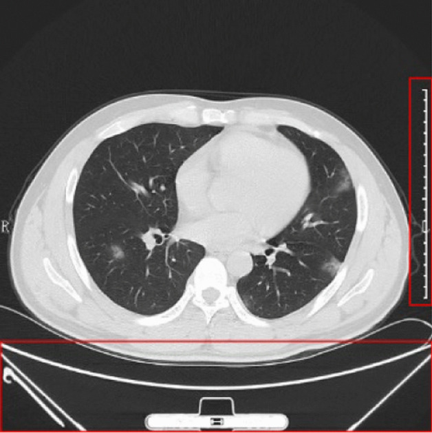
Why we need to crop the chest CT image (the right and bottom show unrelated contents, outlined by red boxes)

The third step: We resize the image to [224, 224]. The reasons are the following: (i) Original size is too large and contains redundant spatial information, (ii) reduced size can accelerate deep neural network processing, and (iii) $224\times 224$ is the standard input for following DenseNet input. After resizing, we get the image set $\mathbb{R}$ from $\mathbb{Z}$. Figure 2 shows an illustration of the preprocessed images in our dataset we shall use in this study.

$$\begin{array}{c}R=Resize\left(\mathbb{Z},,,\left[224224\right]\right)\\ =\left\{r,,,r_2,,,\cdots ,,,r_n\right\}\end{array}$$ 8

Fig. 2.

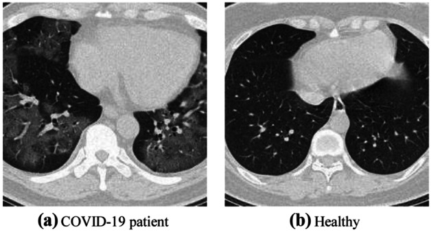
Illustration of preprocessed COVID-19 dataset

The resizing procedure can save storage memory significantly. Suppose we store each image in single-precision floating-point (SPFP) format, i.e., 32 bits = 4 byte the original size for each image is $1024\times 1024\times 3\times 4=12,582,912\mathrm{byte}$. After resizing, the storage for each image is $224\times 224\times 3\times 4=602,112\mathrm{byte}$. Using simple math, we find the resizing procedure can save $1-\frac{602,112}{12,582,912}=95.21\%$ storage, and therefore, we can store all the chest CT images in the RAM, so as to accelerate the running speed of proposed algorithms.

Improvement II: Data Augmentation on Training Set

To avoid overfitting, five disparate data augmentation (DA) techniques were utilized to expand training set. Suppose the dataset $\mathbb{R}$ is divided as three parts: training set $X$ and validate set Y and test set Z via random hold-out (RHO) method

$$\mathbb{R}\stackrel{\mathrm{RHO}}{\to }\left\{X,,,Y,,,Z\right\}$$ 9

where

$$\begin{array}{c}X=\left\{x,(,i,)\right\}\\ Y=\left\{y,(,i,)\right\}\\ Z=\left\{z,(,i,)\right\}\end{array}$$ 10

and their sizes obey following equation

$$\left|X\right|+\left|Y\right|+|Z|=|\mathbb{R}|$$ 11

where $\left|.\right|$ means the cardinality of the set.

In total, we have collected 640 lung window images from chest CT. Afterwards, we use the random hold-out (RHO) method. About 50% were used for training randomly, 20% for validation, and the rest 30% were used for test. The summary of the dataset is listed in Table 3.

Table 2.

RHO setting

Set	COVID-19	Healthy	Total
Training (50%)	160	160	320
Validation (20%)	64	64	128
Test (30%)	96	96	192
Total	320	320	640

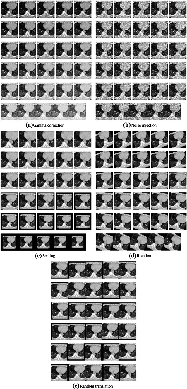
For each image x_i, we perform following five DA operations: (i) Scaling. Chest CT images are scaled with scaling factor s from 0.7 to 1.3 with increase of 0.02, skipping s = 1.

$$\begin{array}{c}\overrightarrow{x^{\mathrm{scale}}(i)}=scale\left[x,(,i,)\right]\\ =\left[x_1^{\mathrm{scale}},\left(i,,,s_1\right),,,\cdots ,x_{30}^{\mathrm{scale}},\left(i,,,s_{30}\right)\right]\end{array}$$ 12

where

$$\begin{array}{c}\begin{array}{c}{s}_1=0.7,s_2=0.72,\cdots ,s_{15}=0.98\\ s_{16}=1.02,\cdots ,s_{30}=1.3\end{array}\end{array}$$ 13

(ii) Rotation. Angle θ was in the value from − 30 to 30° in increase of 2°, skipping $\theta =0$.

$$\begin{array}{c}\overrightarrow{x^{\mathrm{rot}}(i)}=rotate\left[x,(,i,)\right]\\ =\left[x_1^{\mathrm{rot}},\left(i,,,{\theta }_1\right),,,x_2^{\mathrm{rot}},\left(i,,,{\theta }_2\right),,,\cdots ,x_{30}^{\mathrm{rot}},\left(i,,,{\theta }_{30}\right)\right]\end{array}$$ 14

Where

$$\begin{array}{c}{\theta }_1=-{30}^{\circ },{\theta }_2=-{28}^{\circ },\cdots ,{\theta }_{15}=-2^{\circ }\\ {\theta }_{16}=2^{\circ },\cdots ,{\theta }_{30}={30}^{\circ }\end{array}$$ 15

(iii) Noise injection. The m-mean n-variance Gaussian noises [12] are added to the chest CT images $x_i$ to produce 30 new noised images.

$$\begin{array}{c}\overrightarrow{x^{\mathrm{noise}}(i)}=\text{noise}\underset{\_}{}\text{inject}\left[x,(,i,)\right]\\ =\left[x_1^{\mathrm{noise}},\left(i,,,m_1,,,n_1\right),,,\cdots ,x_{30}^{\mathrm{noise}},\left(i,,,m_{30},,,n_{30}\right)\right]\end{array}$$ 16

where

$$m_1=m_2=\cdots =m_{30}=0$$ 17

$$n_1=n_2=\cdots =n_{30}=0.01$$ 18

(iv) Random translation. The chest CT image $x_i$ is translated 30 times with random shift, of which the horizontal and vertical values t = [t_x, t_y] are in the range of [− 15, 15] pixels, and obey uniform distribution $\mathcal{U}$.

$$\begin{array}{c}\overrightarrow{x^{\mathrm{translate}}(i)}=translate\left[x,(,i,)\right]\\ =\left[x_1^{\mathrm{translate}},\left(i,,,t_1\right),,,\cdots ,x_{30}^{\mathrm{translate}},\left(i,,,t_{30}\right)\right]\end{array}$$ 19

where

$$\begin{array}{c}{t}_x\sim \mathcal{U}\left[-,15,15\right]\\ t_y\sim \mathcal{U}\left[-,15,15\right]\end{array}$$ 20

(v) Gamma correction. The gamma correction factor r varies from 0.4 to 1.6 with increase of 0.04, skipping the value of 1

$$\begin{array}{c}\overrightarrow{x^{\mathrm{Gamma}}(i)}=Gamma\_correct\left[x,(,i,)\right]\\ =\left[x_1^{\mathrm{Gamma}},\left(i,,,r_1\right),,,\cdots ,x_{30}^{\mathrm{Gamma}},\left(i,,,r_{30}\right)\right]\end{array}$$ 21

where

$$\begin{array}{c}{r}_1=0.4,r_2=0.44,\cdots ,r_{15}=0.96\\ r_{16}=1.04,\cdots ,r_{30}=1.6\end{array}$$ 22

Finally, horizontal mirror [13] was inducted to all the 150 new generated images.

$$\overrightarrow{x^{\mathrm{mirror}}(i)}=\mathrm{horizontal}\_\mathrm{mirror}\left(\overrightarrow{x^{DA5}(i)}\right)$$ 23

where $\overrightarrow{x^{DA5}}$ means the concatenation of five temporary DA results.

$$\overrightarrow{x^{DA5}(i)}=\mathrm{concat}\left[\begin{array}{c}\overrightarrow{x^{\mathrm{scale}}(i)}\\ \overrightarrow{x^{\mathrm{rot}}(i)}\\ \overrightarrow{x^{\mathrm{noise}}(i)}\\ \overrightarrow{x^{\mathrm{translate}}(i)}\\ \overrightarrow{x^{\mathrm{Gamma}}(i)}\end{array}\right]$$ 24

Thus, one original image will lead to 301 images. Suppose size function is $S$, we have $S\left[x,(,i,)\right]=1$, $S\left[\overrightarrow{x^{DA5}\left(i\right)}\right]=5\times 30=150$, and $S\left[\overrightarrow{x^{\mathrm{mirror}}(i)}\right]=150$. Thus, adding up we get $1+150+150=301$.

$$x(i)\stackrel{\mathrm{DA}}{\to }\mathrm{concat}\left[x,\left(i\right),,,\overrightarrow{x^{DA5}\left(i\right)},,,\overrightarrow{x^{\mathrm{mirror}}(i)}\right]$$ 25

There are other DA techniques, such as color jittering and shear transform. In this study, we choose above five DA techniques, because they can efficiently improve the performances of our established deep learning model. Using other DA techniques may even further improve the performance, and we will leave it as our future studies.

Using Fig. 2a as an example, we can generate in total 150 new images and another 150-image of horizontally flipped images. Figure 3a–e show the $\overrightarrow{x^{\mathrm{DA}5}}$ results. For the page limit, we do not display the horizontally flipped images. After data augmentation, the training set will be $301\times$ of its original size. That means, we have $320\times 301=96,320$ training images in the augmented training set.

Fig. 3.

Data-augmented training samples (mirror results were not shown)

Basics of Transfer learning

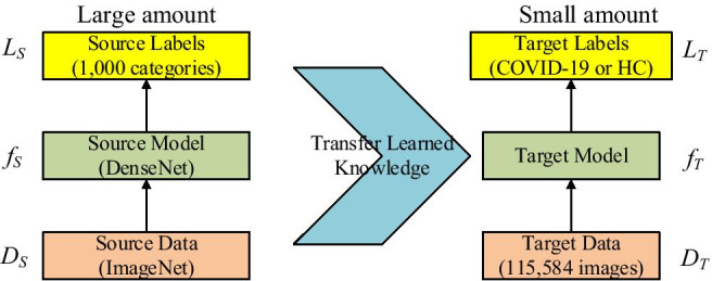
The basic ideas of transfer learning (abbreviated as TL) [14] are utilizing a complicated and successfully pre-trained model (DenseNet in this study), taught from a sizable amount of source data, viz., ImageNet, and then “transfer” the learnt knowledge to the relatively simple task (classify COVID-19 from HC) with a tiny quantity of data. Mathematically, suppose the source data is $D_S$ representing ImageNet, and the source label $L_S$ the 1000-category labeling

$$\mathcal{S}=\left\{D_S,,,L_S,,,f_S\right\}$$ 26

where $f_S$ means the source objective-predictive function, i.e., DenseNet in this study. Now we have the target triple: target data $D_T$ represents the augmented training set, $L_T$ presents the 2-class labeling (COVID-19 or health), and $f_T$ represents the classifier to be established.

$$\mathcal{T}=\left\{{D_T,L}_T,,,f_T\right\}$$ 27

Using transfer learning, the classifier to be created can be written as $f_T\left(D_T,,,L_T,|,D_S,,,L_S,,,f_S\right)=f_T\left(D_T,,,L_T,|\mathcal{S}\right)$. Without transfer learning, the classifier is written as $f_T\left(D_T,,,L_T\right)$. $f_T\left(D_T,,,L_T,|\mathcal{S}\right)$ is expected to be much closer to the ideal classifier $f_T^{\mathrm{Ideal}}$ than using only the target domain, viz. suppose there is a large number of samples $X$, then

$$\begin{array}{c}\left|f_T,\left(D_T,,,L_T,|\mathcal{S}\right),\left(X\right),-,f_T^{\mathrm{Ideal}},\left(X\right)\right|\\ <\left|f_T,\left(D_T,,,L_T\right),\left(X\right),-,f_T^{\mathrm{Ideal}},\left(X\right)\right|\end{array}$$ 28

where | | is some error function over all the samples $X$.

In practice, three elements are vital to help the transfer: (i) The triumph of PTM helps the user get rid of hyper-parameter tuning. (ii) The initial layers in PTM can be thought as feature descriptors which extract low-level features, e.g., tints, edges, blobs, shades, and textures. (iii) The target model may only need to re-train the last several layers of pre-trained model, since we believe the last several layers carry out the complex identification tasks. The basic idea of transfer learning is shown in Fig. 4.

Fig. 4.

Idea of transfer learning

Improvement III: Use DenseNet as Backbone

Pretrained models (PTMs) are useful tools to help the AI practitioners to swiftly develop a deep neural network suitable for a specific task. Common PTMs include AlexNet, VGGNet, ResNet, GoogleNet, and DenseNet. AlexNet was proposed by [15], which overwhelmed the other competitor models in the competition of ImageNet Large Scale Visual Recognition Challenge (ILSVRC) at year 2012. The structure of AlexNet is similar to LeNet but with some new techniques like local response normalization (LRN), max pooling, and ReLU nonlinearity. [16] presented VGGNet that was a 19-layer deep neural network and won the 2nd place of ILSVRC-2014. GoogleNet was proposed by [17] combined some new ideas including $1\times 1$ convolutions, reducing size of feature maps and making the network deeper and wider. The winner ResNet [18] of ILSVRC-2015 presented a deeper network with 152 layers, which includes a new idea of a shortcut connection. Then in 2016, [19] developed a new idea so called “DenseBlock (DB),” which introduced the feature reuse into the whole network.

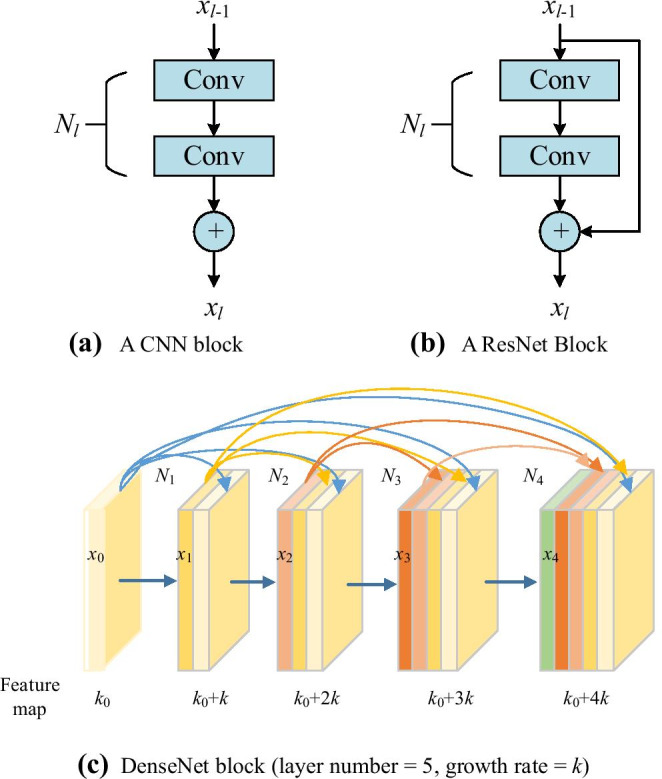
In this study, we choose DenseNet as the backbone for developing a smart COVID-19 diagnosis system, as DenseNet provides the best performance based on the ImageNet classification task. In the traditional CNN shown in Fig. 5a, all layers are gradually connected as

$$\mathrm{CNN}:x_l=N_l(x_{l-1})$$ 29

Fig. 5.

Comparison of plain CNN block, ResNet block, and DenseNet block

where l stands for the layer index and N means the non-linear operation. x_l represents the feature from of the $l_{\mathrm{th}}$ layer. CNN makes the network challenging to go wider and deeper, as it may face problems of either exploding or gradient vanishing. Then, ResNet employed the shortcut connection by skipping at least two layers.

$$\mathrm{ResNet}:x_l=N_l(x_{l-1})+x_{l-1}$$ 30

Figure 5b shows its structure, of which the input is x_l − 1 and the output after two conv layers N_l(x_l − 1) is added with the shortcut to input layer x_l − 1, and thus, the summation is the output of l-th layer.

Further, DenseNet block shown in Fig. 5c revises the model by concatenating all the feature maps $[x_0,x_1,...,x_{l-1}]$ sequentially instead of summation of the output feature maps from all previous layers

$$\mathrm{DenseNet}:x_l=N_l(\mathrm{concat}[x_0,x_1,...,x_{l-1}])$$ 31

DenseNet offers concatenations of all feature maps from previous layers [20], which means, all the feature maps propagate to the later layers and connected to the newly generated feature maps. The new developed DenseNet introduce some advantages like feature reuse, decrease the problem of either exploding or gradient vanishing [21].

From Fig. 5c, we find that k feature maps are generated for each operation $N_l$.

$$\begin{array}{c}\begin{array}{c}{x}_1=N_1\left(x_0\right)\\ x_2=N_2\left(\mathrm{concat},\left[x_0,,,x_1\right]\right)\\ x_3=N_3\left(\mathrm{concat},\left[x_0,,,x_1,,,x_2\right]\right)\end{array}\\ x_4=N_4\left(\mathrm{concat},\left[x_0,,,x_1,,,x_2,,,x_3\right]\right)\end{array}$$ 32

As there are five layers in Fig. 5c, we can get k₀ + 4 k feature maps finally as the final feature map is $[x_0,x_1,x_2,x_3,x_4]$; k₀ stands for the number of feature map ($x_0$) from previous layer. The default value of k in this study is 32.

Note that there are a large number of inputs of the network; a bottleneck layer was introduced to the DenseNet, which is implemented by a 1 × 1 convolution before the 3 × 3 convolution layer, which is helpful in reducing the feature maps and saving the computation cost [22].

Transition layers (TLs) were proposed among DenseBlocks. TL has two advantages: (i) It can compress the number of feature maps: suppose k feature maps are generated by a DenseBlock and assume the compression factor as $\theta \in (0,1]$. Then the feature maps $N_{\mathit{FM}}$ will be reduced to ⌊$\theta \times k\rfloor$.

$$N_{\mathrm{FM}}=\left\{\begin{array}{cc}k& \mathrm{before}\mathrm{TL}\\ \lfloor \theta \times k\rfloor & \mathrm{after}\mathrm{TL}\end{array}\right)$$ 33

If $\theta$ = 1, the number of feature maps will be the same.

(ii) It can downsample the feature maps within the transition layers, i.e., $1\times 1$ conv followed by $2\times 2$ pooling between two consecutive DenseBlock. Feature map sizes are the same within each dense block so that they can be concatenated together easily.

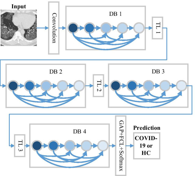
Figure 6 shows the operations in transition layers: batch normalization, convolution, and pooling operations.

Fig. 6.

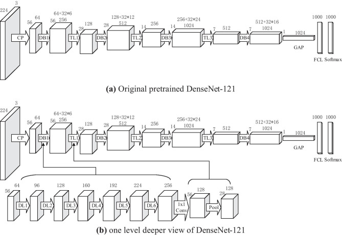
How DenseNet classify chest CT images (TL transition layer, DB DenseBlock, GAP global average pooling, FCL fully connected layer)

Figure 6 illustrates the structure of DenseNet, which includes three DBs, input layer, TLs, and global average pooling (GAP) layer. The TLs consist of a batch normalization layer, a 1 × 1 conv layer and a 2 × 2 average pooling layer with stride of 2. Particularly, the GAP is similar to traditional maximum pooling (MP) and average pooling (AP) methods, but it undertakes a more extreme feature map reduction, that reduces the size of feature map $S_{\mathrm{FM}}$ from $\omega \times \omega \times c$ to 1 × 1 × c.

$$S_{\mathrm{FM}}=\left\{\begin{array}{cc}\omega \times \omega \times c& \mathrm{before}\mathrm{GAP}\\ 1\times 1\times c& \mathrm{after}\mathrm{GAP}\end{array}\right)$$ 34

That means, GAP layer reduces the whole slice into a single digit.

We needed to modify the structure of DenseNet before making it feasible for our COVID-19 diagnosis task. The last dense layer, viz., FCL was modified, since original last FCL was created to classify 1000 categories, of which 20 randomly ones are listed below: recreational vehicle, printer, coho, milk can, Irish wolfhound, parallel bars, tree frog, dhole, Gila monster, toucan, spider web, organ, walking stick, broccoli, loggerhead, bassoon, colobus, racket, schooner, and Kerry blue terrier. We can observe that none of those 20 categories are related to chest CT or COVID-19, which were the main classification task in this study.

Because the size of output neurons in standard DenseNet (1000-way) does not equal the number of classes in this study (two-way as COVID-19 and healthy control), it is necessary to modify the last FCL and the classification layer.

The modification is presented in Table 2. In this TL environment, a new randomly initialized FCL with 2 output neurons, and a new classification layer with 2 categories (COVID-19 and HC), was used to replace the previous cognate layers. The parameters of softmax layer were updated accordingly.

Table 3.

Modification of layers of DenseNet

Layer	Original	Replaced
Third from last	FCL (1000) with pre-trained weights and biases	FCL (2) with random initialization
Last	Classification Layer 1000 classes: recreational vehicle, printer, coho, milk can, Irish wolfhound, parallel bars, tree frog, dhole, Gila monster, toucan, spider web, organ, walking stick, broccoli, loggerhead, bassoon, colobus, racket, schooner, and Kerry blue terrier, and 980 other classes	Classification Layer Two classes: (i) COVID-19; (ii) Healthy control

Improvement IV: Optimization of TL Setting

How to optimize the DenseNet transfer learning setting? There are many hyperparameters need to determine, e.g., do we use DenseNet-121, DenseNet-169, or DenseNet-201? How to we divide the frozen layers, middle layers, and new layers? To solve above issues, we propose an optimization of transfer learning setting (OTLS) framework in this study.

Take DenseNet-121 shown in Fig. 7a as an example, it contains the 121 learnable layers: (6 + 12 + 24 + 16) ∗ 2 = 116 layers in the dense blocks and 5 layers from first conv layer, last FCL, and three TLs. The details of DenseNet-121 are shown in Table 4. Figure 7b shows the inner structure of blocks DB1 and TL1.

Fig. 7.

Structure of DenseNet-121 (CP means the first block of conv layer and pooling layer, DB means the dense block, TL means the transition layer, GAP means global average pooling, FCL means fully connected layer, DL means dense layer)

Table 4.

Detailed information of each layer/block in DenseNet-121

Index	Layers	DenseNet-121	Output
1	Input		224 × 224 × 3
2	Conv	7 × 7/2 conv,	112 × 112 × 64
3	Pooling	3 × 3/2 MP	56 × 56 × 64
4	DB1	$\left[\begin{array}{cc}1\times 1& \text{conv}\\ 3\times 3& \text{conv}\end{array}\right]\times 6$	56 × 56 × 256
5	TL1	1 × 1 conv, 2 × 2/2 AP	28 × 28 × 128
6	DB2	$\left[\begin{array}{cc}1\times 1& \text{conv}\\ 3\times 3& \text{conv}\end{array}\right]\times 12$	28 × 28 × 512
7	TL2	1 × 1 conv, 2 × 2/2 AP	14 × 14 × 256
8	DB3	$\left[\begin{array}{cc}1\times 1& \text{conv}\\ 3\times 3& \text{conv}\end{array}\right]\times 24$	14 × 14 × 1024
9	TL3	1 × 1 conv, 2 × 2/2 AP	7 × 7 × 512
10	DB4	$\left[\begin{array}{cc}1\times 1& \text{conv}\\ 3\times 3& \text{conv}\end{array}\right]\times 16$	7 × 7 × 1024
11	Pooling	7 × 7/7 GAP	1 × 1 × 1024
12	FCL	1000 days	1 × 1 × 1000

DB dense block, TL transition layer, FCL fully connected layer

For DenseNet-201, traditional transfer learning uses simple learning factor (SLF), which employs the same learning factor across all the layers within a neural network. This study employs an advanced strategy called composite learning factor (CLF) [23]: the early transferred layers are frozen with learning factor ${\mathrm{LF}}_{\mathrm{Frozen}}=0$, i.e., no update, the middle transferred-layers are updated slowly with LF of 1, and the final added new layers learn fast with LF of 10. From the overall viewpoint, there are four different composite-learning-factor-settings (CLFSs) for DenseNet. Table 5 shows the detailed information of CLFSs.

Table 5.

Composite-learning factor setting

CLFS	Frozen layers	Middle layers	New layers
	${\mathrm{LF}}_{\mathrm{Frozen}}=0$	${\mathrm{LF}}_{\mathrm{Middle}}=1$	${\mathrm{LF}}_{\mathrm{New}}=10$
I	CP, DB1, TL1, DB2	TL2, DB3, TL3, DB4	FCL
II	CP, DB1, TL1, DB2, TL2	DB3, TL3, DB4	FCL
III	CP, DB1, TL1, DB2, TL2, DB3	TL3, DB4	FCL
IV	CP, DB1, TL1, DB2, TL2, DB3, TL3	DB4	FCL

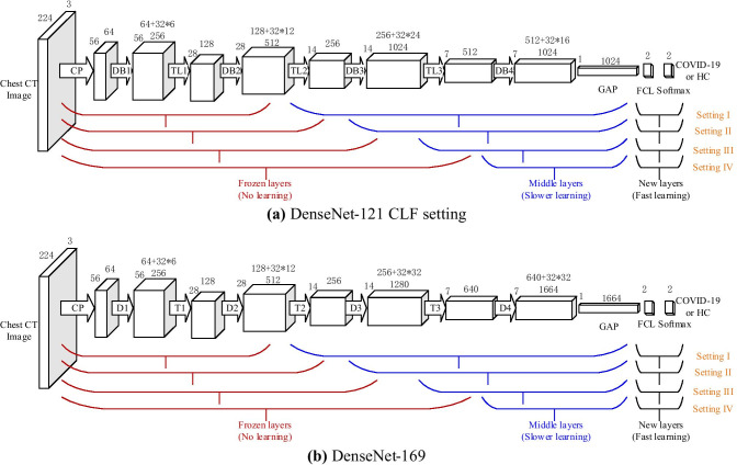
The LF of final new layers is ten times of that of middle transferred-layer, for the middle transferred-layers are with pre-trained weights/biases and new layers are with random-initialized weights/biases. Its structure is shown in Fig. 8a. Here CLF Setting III means the layers from CP to DB3 are frozen. The layers from TL3 to DB4 are transferred directly with pre-trained weights, and they are updated with learning factor ${\mathrm{LF}}_{\mathrm{Middle}}=1$; note that the learning rate (LR) equals global learning rate (GLR) times learning factor (LF).

$$\mathrm{LR}=\mathrm{GLR}\times \mathrm{LF}$$ 35

Fig. 8.

CLF Setting

The final new layers of FCL are randomly initialized with ${\mathrm{LF}}_{\mathrm{New}}=10$. In all, LF is chosen as

$$\mathrm{LF}=\left\{\begin{array}{cc}0& \text{Fronzen Layers}\\ 1& \text{Middle Layers}\\ 10& \text{New Layers}\end{array}\right)$$ 36

We can observe that LF has three possible associated values to frozen layers, middle layers, and new layers. The LF value configurations of ${\mathrm{LF}}_{\mathrm{Frozen}}=0$, ${\mathrm{LF}}_{\mathrm{Middle}}=1$, and ${\mathrm{LF}}_{\mathrm{New}}=10$ are obtained from Wang [23]. To test other combination values of $\left({\mathrm{LF}}_{\mathrm{Frozen}},,,\mathrm{L},{\mathrm{F}}_{\mathrm{Middle}},,,\mathrm{L},{\mathrm{F}}_{\mathrm{New}}\right)$ is one of our further research directions.

Except to optimize the CLF setting, we also need to seek for the optimal DenseNet structure. There are currently three stable DenseNet models: DenseNet-121, DenseNet-169, and DenseNet-201. Those three models have similarity structures with DenseNet-121, except that the number of 1 × 1 and 3 × 3 layers. For DenseNet-121, it contains 24 and 16 subblocks in Dense Block 3 and 4, respectively. For DenseNet-169, as shown in Fig. 8b, it includes 32 subblocks in Dense Block both 3 and 4. For DenseNet-201, the numerals change to 48 and 32 within Dense Block 3 and 4, respectively. Figure 8 shows the CLF settings of DenseNet-121 and DenseNet-169 adapted to our COVID-19 diagnosis task.

Precomputation Analysis

Precomputation is employed here. After freezing the layers by setting their cognate learning factor to 0, we can calculate the activation maps at the last frozen layer for all the images in the dataset. Then we save the feature maps to hard drive storage. Those feature maps are used as input images to train the trainable layers (middle layers and new layers in Table 5), which can be regarded as a smaller standalone neural network.

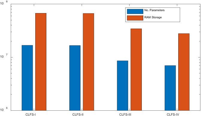
Using DenseNet-201 as example, we check the RAM storage. Again, we assume parameters are stored in the format of SPFP format (4 bytes). We can have the storage comparison of all four CLF settings (considering weights, biases, offsets, scales, etc.) in Fig. 9, where y-axis uses log scale for ease of view. We can see CLFS-IV only costs parameters of 6.98 million, and the memory storage of around 27.95 MB, which are the least values of all CLF settings.

Fig. 9.

Storage comparison of four transfer learning settings in DenseNet-201

Implementation

The experiment ran ten times. At each time, the training-validation hold-out division was reset at random. The test set was kept away from training at the very beginning, so its information would not be leaked to the training procedure. The training stopped when either it reached given maximum epoch, or the validation performance ${\mathcal{P}}_{\mathrm{val}}$ decreased over preset training epochs. Stochastic gradient descent with momentum (SGDM) approach was selected as the training algorithm

Table 6 shows the pseudocode of proposed DenseNet-OTLS method. In Phase I, we use the preprocessing approaches described in “Improvement I: Preprocessing” to make the data tractable and fit our deep neural network model. In Phase II, we use the proposed OTLS frame to seek the optimal base smodel (BM) and composite learning factor setting (CLFS). The core function here is “TrainNetwork” with four arguments: (i) BM $M$, (ii) CLFS S, (iii) train data t, and (v) validation data v.

$$\mathbb{M}=\mathrm{TrainNetwork}(\mathrm{BM},\mathrm{CLFS},t,v)$$ 37

Table 6.

Pseudocode of our proposed DenseNet-OTLS method

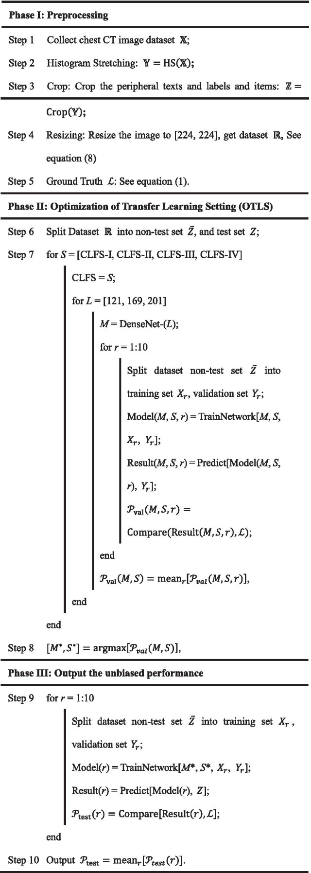
Using the trained model and new data, we can get the prediction results $\mathrm{\gamma }$ on particular data d by the model $\mathbb{M}$.

$$\mathrm{\gamma }=\mathrm{Predict}(\mathbb{M},d)$$ 38

With the ground truth labels $\mathcal{L}$, we can calculate the performance $\mathcal{P}$.

$$\mathcal{P}=\mathrm{Compare}(\mathrm{\gamma },\mathcal{L})$$ 39

The performance can be training performance ${\mathcal{P}}_{\mathrm{train}}$, or validation performance ${\mathcal{P}}_{\mathrm{val}}$, or test performance ${\mathcal{P}}_{\mathrm{test}}$, based on the properties of data d. The optimal BM $M^{\ast }$ and optimal CLSF $S^{\ast }$ can be obtained on validation set by

$${[M}^{\ast },S^{\ast }]=\mathrm{argmax}\left[{\mathcal{P}}_{\mathrm{val}},(M,S)\right]$$ 40

In Phase III, “Predict” function was conducted on the test set, and we will finally get the test performance ${\mathcal{P}}_{\mathrm{test}}$.

Indicators

The test performances across all 10 runs were noted, and the six indicators were assessed: sensitivity (SEN), specificity (SPC), accuracy (ACC), precision (PRC), F1 score, and Matthews correlation coefficient (MCC). We used those six indicators because they are widely reported I recent literature. There are some other indicators, but we did not use them, since we believed these six indicators were sufficient to measure the performance of proposed classifiers.

Assume positive means COVID-19, and negative means healthy control. The first four measures were defined as

$$\mathrm{SEN}=\frac{\mathrm{TP}}{\mathrm{TP}+\mathrm{FN}}$$ 41

$$\mathrm{SPC}=\frac{\mathrm{TN}}{\mathrm{TN}+\mathrm{FP}}$$ 42

$$\mathrm{PRC}=\frac{\mathrm{TP}}{\mathrm{TP}+\mathrm{FP}}$$ 43

$$\mathrm{ACC}=\frac{\mathrm{TP}+\mathrm{TN}}{\mathrm{TP}+\mathrm{TN}+\mathrm{FP}+\mathrm{FN}}$$ 44

where TP, FP, TN, and FN represent true positive, false positive, true negative, and false negative, respectively. F1 and MCC are defined as

$$\begin{array}{c}{F}_1={\left(\frac{{\mathrm{SEN}}^{-1}+{\mathrm{PRC}}^{-1}}{2}\right)}^{-1}\\ =\frac{2\times \mathrm{TP}}{2\times \mathrm{TP}+\mathrm{FP}+\mathrm{FN}}\end{array}$$ 45

$$\mathrm{MCC}=\frac{\mathrm{TP}\times \mathrm{TN}-\mathrm{FP}\times \mathrm{FN}}{\sqrt{\left(\mathrm{TP},+,\mathrm{FP}\right)\times \left(\mathrm{TP},+,\mathrm{FN}\right)\times \left(\mathrm{TN},+,\mathrm{FP}\right)\times (\mathrm{TN}+\mathrm{FN})}}$$ 46

The MCC was used in machine learning as an indicator for binary classification since 1975. MCC itself is a correlation coefficient between observation and prediction. Its value is between − 1 and 1, i.e., $-1\le \text{MCC}\le 1$. When MCC equals to − 1, 0, and 1, the corresponding meanings are shown below as

$$\mathrm{MCC}=\left\{\begin{array}{cc}1& \text{perfect classification}\\ 0& \text{random prediction}\\ -1& \text{totally wrong classification}\end{array}\right)$$ 47

The average and standard deviation (SD) of six indicators of ten runs on the test set were analyzed and used for comparison. Two important global hyperparameters were set below: (i) the number of training epochs was set to 10, since the whole training procedure of a transfer learning should be swift. (ii) The global learning rate (GLR) was set to a trivial value of 10^–4 to slow down learning, because transfer learning will be carried out on a pre-trained DenseNet model.

Results and Discussions

Optimization of Transfer Learning Setting

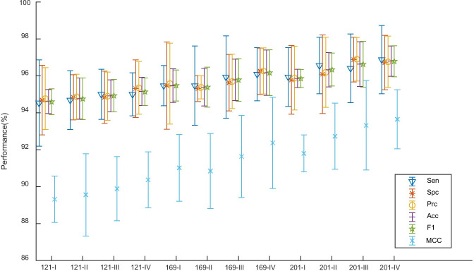
For the three DenseNet variants and four CLF settings, the comparison results were listed in Table 7. The best two are DenseNet-201-CLFS-III and DenseNet-201-CLFS-IV. The former obtains a sensitivity of 96.41 ± 1.86%, a specificity of 96.88 ± 1.21%, a precision of 96.90 ± 1.18%, an accuracy of 96.64 ± 1.21%, an F1 score of 96.63 ± 1.24%, and an MCC of 93.32 ± 2.42%. The latter one produces a sensitivity of 96.88 ± 1.85%, a specificity of 96.72 ± 1.47%, a precision of 96.76 ± 1.39%, an accuracy of 96.80 ± 0.82%, an F1 score of 96.79 ± 0.84%, and an MCC of 93.65 ± 1.60%. Considering CLFS IV will use less storage, we finally choose “201-IV” as our best model.

Table 7.

Validation performance based on the best configuration (unit: %)

Run	Sen	Spc	Prc	Acc	F1	MCC
R1	98.44	96.88	96.92	97.66	97.67	95.34
R2	93.75	98.44	98.39	96.09	96.01	92.30
R3	98.44	93.75	94.03	96.09	96.18	92.30
R4	96.88	96.88	96.88	96.88	96.88	93.75
R5	98.44	95.31	95.45	96.88	96.92	93.80
R6	98.44	98.44	98.44	98.44	98.44	96.88
R7	95.31	98.44	98.44	96.88	96.82	93.84
R8	93.75	96.88	96.77	95.31	95.21	90.71
R9	96.88	96.88	96.87	96.88	96.85	93.80
R10	98.44	95.31	95.45	96.88	96.92	93.80
Mean ± SD	96.88 ± 1.85	96.72 ± 1.47	96.76 ± 1.39	96.80 ± 0.82	96.79 ± 0.84	93.65 ± 1.60

Figure 10 shows the error bar plot of ${\mathcal{P}}_{\mathrm{val}}$, showing that DenseNet-201 yields better performances than DenseNet-121 and DenseNet-169 overall. The reason may be because DenseNet-201 has the deepest neural structure; thus, it can map more complicated patterns, such as the ground-glass opacity (GGO) lesions of a chest CT image of COVID-19 patients.

Fig. 10.

Error bar of validation performances

The detailed information of 10 runs of the best model “201-IV” is shown in Table 8. Each row shows the result of one run. The last row shows the mean and standard deviation of all 10 runs. From the last row, we can see the standard deviation values of accuracy and F1 are much smaller than those of other four indicators.

Table 8.

Validation performance ${\mathcal{P}}_{\mathbf{v}\mathbf{a}\mathbf{l}}$ (Unit: %)

Model	CLFS	Sensitivity	Specificity	Precision	Accuracy	F1	MCC
DenseNet-121	I	94.53 ± 2.34	94.69 ± 1.88	94.77 ± 1.67	94.61 ± 0.65	94.60 ± 0.70	89.32 ± 1.25
	II	94.69 ± 1.59	94.84 ± 1.22	94.87 ± 1.22	94.77 ± 1.11	94.76 ± 1.13	89.56 ± 2.23
	III	95.00 ± 1.36	94.84 ± 1.41	94.90 ± 1.31	94.92 ± 0.87	94.93 ± 0.88	89.89 ± 1.74
	IV	95.00 ± 1.17	95.31 ± 1.56	95.35 ± 1.43	95.16 ± 0.77	95.14 ± 0.75	90.37 ± 1.52
DenseNet-169	I	95.47 ± 1.09	95.47 ± 2.36	95.58 ± 2.19	95.47 ± 0.91	95.48 ± 0.84	91.02 ± 1.81
	II	95.47 ± 2.15	95.31 ± 0.70	95.38 ± 0.63	95.39 ± 1.02	95.39 ± 1.08	90.85 ± 2.03
	III	95.94 ± 2.23	95.63 ± 1.53	95.70 ± 1.47	95.78 ± 1.12	95.78 ± 1.15	91.64 ± 2.22
	IV	96.09 ± 1.44	96.25 ± 1.25	96.27 ± 1.25	96.17 ± 1.23	96.17 ± 1.24	92.37 ± 2.47
DenseNet-201	I	95.94 ± 1.59	95.78 ± 1.86	95.88 ± 1.73	95.86 ± 0.50	95.86 ± 0.49	91.80 ± 1.00
	II	96.56 ± 1.53	96.09 ± 2.13	96.19 ± 1.90	96.33 ± 0.93	96.34 ± 0.89	92.73 ± 1.79
	III	96.41 ± 1.86	96.88 ± 1.21	96.90 ± 1.18	96.64 ± 1.21	96.63 ± 1.24	93.32 ± 2.42
	IV	96.88 ± 1.85	96.72 ± 1.47	96.76 ± 1.39	96.80 ± 0.82	96.79 ± 0.84	93.65 ± 1.60

Performance on Test Set via “201-IV”

Since we have determined from the validation set that the optimal combination is “201-IV,” we run this proposed model on the test set for 10 new runs, with results of each run shown in Table 9.

Table 9.

Test performance ${\mathcal{P}}_{\mathbf{t}\mathbf{e}\mathbf{s}\mathbf{t}}$ based on best model “201-IV” found by proposed DenseNet-OTLS (unit: %)

Run	Sen	Spc	Prc	Acc	F1	MCC
R1	96.88	96.88	96.94	96.88	96.90	93.77
R2	97.92	94.79	94.98	96.35	96.42	92.76
R3	95.83	97.92	97.92	96.88	96.85	93.79
R4	95.83	97.92	97.87	96.88	96.84	93.77
R5	97.92	95.83	95.96	96.88	96.92	93.79
R6	96.88	94.79	94.90	95.83	95.88	91.69
R7	94.79	96.88	96.83	95.83	95.79	91.71
R8	95.83	94.79	94.81	95.31	95.30	90.68
R9	94.79	96.88	96.78	95.83	95.77	91.70
R10	96.88	95.83	95.88	96.35	96.37	92.72
Mean ± SD	96.35± 1.07	96.25± 1.16	96.29± 1.11	96.30± 0.54	96.30± 0.56	92.64± 1.08

The comparison between Table 9 with Table 7 is shown in Fig. 11, from which we can see the following:

Fig. 11.

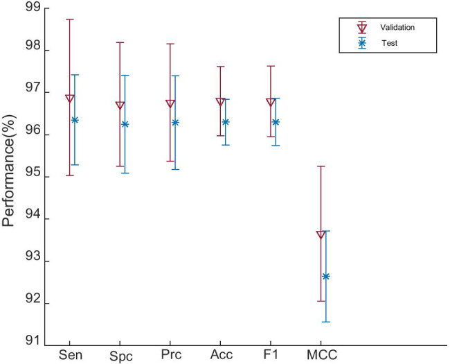
Comparison of validation performance and test performance

(i) The performance on test set ${\mathcal{P}}_{\mathrm{test}}$ is a bit lower than that performance on validation set ${\mathcal{P}}_{\mathrm{val}}$ in terms of all six measures. The reason is the test set is brand new data to the models, but validation set contributes to the trained model. So ${\mathcal{P}}_{\mathrm{val}}$ looks better than ${\mathcal{P}}_{\mathrm{test}}$. (ii) We find the SD on test set is smaller than that on validation set. The reason is because the size of test set is larger than validation set, as can be found in Table 3.

Comparison to State-of-the-Art Approaches

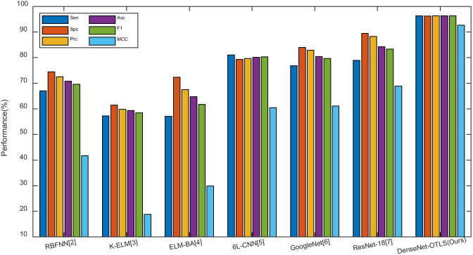
We compare our method “DenseNet-OTLS” with other COVID-19 classification approaches: RBFNN [2], K-ELM [3], ELM-BA [4], 6L-CNN [5], GoogLeNet [6], and ResNet-18 [7]. The comparison results based on test set of 10 runs are shown in Table 10, where it is clear that proposed approach is significantly better than all the six state-of-the-art methods:

Table 10.

Comparison with COVID-19 identification approaches (Unit: %)

Approach	Sen	Spc	Prc	Acc	F1	MCC
RBFNN [2]	67.08	74.48	72.52	70.78	69.64	41.74
K-ELM [3]	57.29	61.46	59.83	59.38	58.46	18.81
ELM-BA [4]	57.08 ± 3.86	72.40 ± 3.03	67.48 ± 1.65	64.74 ± 1.26	61.75 ± 2.24	29.90 ± 2.45
6L-CNN [5]	81.04 ± 2.90	79.27 ± 2.21	79.70 ± 1.27	80.16 ± 0.85	80.31 ± 1.13	60.42 ± 1.73
GoogLeNet [6]	76.88 ± 3.92	83.96 ± 2.29	82.84 ± 1.58	80.42 ± 1.40	79.65 ± 1.92	61.10 ± 2.62
ResNet-18 [7]	78.96 ± 2.90	89.48 ± 1.64	88.30 ± 1.50	84.22 ± 1.23	83.31 ± 1.53	68.89 ± 2.33
DenseNet-OTLS (Ours)	96.35 ± 1.07	96.25 ± 1.16	96.29 ± 1.11	96.30 ± 0.54	96.30 ± 0.56	92.64 ± 1.08

In all, the comparison results of eight methods are shown in Fig. 12. This picture indicates that this proposed DenseNet-OTLS approach can achieve the highest performance among all state-of-the-art approaches.

Fig. 12.

Comparison of our method with seven state-of-the-art approaches

Composite Learning Rate Versus Simple Learning Rate

We compare this composite learning factor (CLF) strategy with traditional simple learning factor (SLF), as described in “Improvement IV: Optimization of TL Setting.” SLF is designed here as that we set the frozen layers with learning factor of 0, and the rest layers with learning factor of 1. We compare our CLF result with SLF and show the comparison in Table 11 and Fig. 13.

Table 11.

Composite learning factor versus simple learning factor (Unit: %)

Setting	Sen	Spc	Prc	Acc	F1	MCC
SLF	94.37 ± 1.06	94.58 ± 1.60	94.62 ± 1.50	94.48 ± 0.78	94.48 ± 0.76	89.00 ± 1.56
CLF(Ours)	96.35 ± 1.07	96.25 ± 1.16	96.29 ± 1.11	96.30 ± 0.54	96.30 ± 0.56	92.64 ± 1.08

Fig. 13.

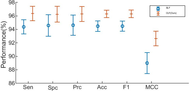
Error bar plot of CLF versus SFL

The results indicate that CLF yields better performance than SLF. The reason is all the layers are divided into three types (FL, ML, and NL) using CLF: (i) frozen layers (FLs) inherit structure and weights from pretrained models; (ii) middle layers (MLs) inherit network structure, and use pretrained weights as initial; and (iii) newly layers (NLs) have no relevancy with PTMs.

Effect of Preprocessing

We justify the effectiveness of preprocessing in this experiment. Remember our preprocessing consists of three steps: (i) HS, (ii) crop, and (iii) resize. Suppose we do not do this three-step preprocessing, i.e., we only carry out the resizing due to the transfer learning requirement. The comparison is carried out over test set and the results are itemized in Table 12.

Table 12.

Effectiveness of proposed three-step preprocessing

Setting	Sen	Spc	Prc	Acc	F1	MCC
Only resizing	93.33 ± 2.21	91.77 ± 2.75	91.94 ± 2.55	92.55 ± 2.07	92.61 ± 2.02	85.14 ± 4.13
Preprocessing (Ours)	96.35 ± 1.07	96.25 ± 1.16	96.29 ± 1.11	96.30 ± 0.54	96.30 ± 0.56	92.64 ± 1.08

Table 12 indicate that without proper preprocessing (HS and Crop), the performance of the system will decrease to a sensitivity of 93.33 ± 2.21%, a specificity of 91.77 ± 2.75%, and an accuracy of 92.55 ± 2.07%. This comparison clearly indicates the effectiveness of this proposed three-step preprocessing.

Conclusion

This paper proposed a novel COVID-19 diagnosis method based on DenseNet and optimization of transfer learning setting (OTLS) framework. The OTLS includes optimization the composite learning factor setting (CLFS) and optimization the DenseNet structure. The experiments showed our method DenseNet-OTLS is superior to six state-of-the-art approaches.

The shortcomings of this research are two-fold: (i) We did not validate the optimal combination configuration of DA techniques. We shall quantify the effect of each DA technique. (ii) We did not validate the optimal values of $\left({\mathrm{LF}}_{\mathrm{Frozen}},,,\mathrm{L},{\mathrm{F}}_{\mathrm{Middle}},,,{\mathrm{LF}}_{\mathrm{New}}\right)$. We will try to develop some automatic learning factor optimization method.

Furthermore, we shall try to increase COVID-19′s diagnosis performance further. One solution way is to make combination of different transfer learning setting, creating an ensemble DenseNet deep neural network. Another research direction is to output the localization the lesions of COVID-19, which can assist the chest radiologists to make more accurate diagnosis.(see. Table 13)

Highlights

• DenseNet was introduced as the backbone pre-trained model, and we modified it to this COVID-19 diagnosis task.

• Composite learning factor strategy was used for training DenseNet.

• Data augmentation was used to enhance the training set.

• An optimization of transfer learning setting (OTLS) was proposed to search for the optimal optimization setting.

• Precomputation was introduced to save memory.

• We compared proposed DenseNet-OTLS method with state-of-the-art COVID-19 diagnosis approaches.

Appendix

Table 13.

Abbreviations and their full names

Abbreviation	Full name
AP	Average pooling
BM	Base model
CLF	Composite learning factor
CLFS	Composite learning factor setting
CNN	Convolutional neural network
CT	Computed Tomography
DA	Data augmentation
DB	DenseBlock
FCL	Fully connected layer
FL	Frozen layer
GAP	Global average pooling
GGO	Ground-glass opacity
GLR	Global learning rate
HC	Healthy control
HS	Histogram stretching
HU	Hounsfield unit
ILSVRC	ImageNet large scale visual recognition challenge
LF	Learning factor
LR	Learning rate
LRN	Local response normalization
MCC	Matthews correlation coefficient
ML	Middle layer
MP	Maximum pooling
MV	Majority voting
NL	New layer
OTLS	Optimization of transfer learning setting
PCR	Polymerase chain reaction
PTM	Pre-trained model
RHO	Random hold-out
SD	Standard deviation
SGDM	Stochastic gradient descent with momentum
SLF	Simple learning factor
SPFP	Single-precision floating-point
TL	Transfer learning
TL	Transition layer

Funding

This paper is partially supported by Royal Society International Exchanges Cost Share Award, UK (RP202G0230); Medical Research Council Confidence in Concept Award, UK (MC_PC_17171); Hope Foundation for Cancer Research, UK (RM60G0680); Henan Key Research and Development Project (182102310629); Natural Science Foundation of China (61602250, 11502090, U1711263, U1811264); Guangxi Key Laboratory of Trusted Software (kx201901); Natural Science Foundation of Zhejiang Province (Y18F010018); British Heart Foundation Accelerator Award, UK; Fundamental Research Funds for the Central Universities (CDLS-2020-03); and Key Laboratory of Child Development and Learning Science (Southeast University), Ministry of Education.

Compliance with Ethical Standards

Informed Consent

Informed consent was obtained from all individual participants included in the study.

Research Involving Human Participants and/or Animals

All procedures performed in studies involving human participants were in accordance with the ethical standards of the institutional and/or national research committee and with the 1964 Helsinki declaration and its later amendments or comparable ethical standards.

References

- 1.Ai T, et al. Correlation of chest CT and RT-PCR testing in coronavirus disease 2019 (COVID-19) in China: a report of 1014 cases. Radiology. 2020: Article ID. 200642. [DOI] [PMC free article] [PubMed]
- 2.Lu Z. A pathological brain detection system based on radial basis function neural network. J Med Imaging Health Infor. 2016;6(5):1218–22. doi: 10.1166/jmihi.2016.1901. [DOI] [Google Scholar]
- 3.Yang J. A pathological brain detection system based on kernel based ELM. Multimed Tools Appl. 2018;77(3):3715–28. doi: 10.1007/s11042-016-3559-z. [DOI] [Google Scholar]
- 4.Lu S. A pathological brain detection system based on extreme learning machine optimized by bat algorithm. CNS & Neurological Disorders - Drug Targets. 2017;16(1):23–29. doi: 10.2174/1871527315666161019153259. [DOI] [PubMed] [Google Scholar]
- 5.Jiang X. Chinese sign language fingerspelling recognition via six-layer convolutional neural network with leaky rectified linear units for therapy and rehabilitation. J Med Imaging Health Infor. 2019;9(9):2031–8. doi: 10.1166/jmihi.2019.2804. [DOI] [Google Scholar]
- 6.Szegedy C, et al. Going deeper with convolutions. in Proceedings of the IEEE conference on computer vision and pattern recognition. 2015. p. 1–9.
- 7.Yu X, et al. Abnormality diagnosis in mammograms by transfer learning based on ResNet18. Fundam Inform. 2019;168(2–4):219–30. doi: 10.3233/FI-2019-1829. [DOI] [Google Scholar]
- 8.Rajaraman S, et al. Weakly Labeled Data Augmentation for Deep Learning: A Study on COVID-19 Detection in Chest X-Rays. Diagnostics. 2020;10(6): p. 17: Article ID. 358. [DOI] [PMC free article] [PubMed]
- 9.Ni QQ, et al. A deep learning approach to characterize 2019 coronavirus disease (COVID-19) pneumonia in chest CT images. Eur Radiol. 2020: p. 11. [DOI] [PMC free article] [PubMed]
- 10.Novitasari DCR, et al. Detection of covid-19 chest x-ray using support vector machine and convolutional neural network. Commun Math Biol Neurosci. 2020: p. 19: Article ID. 42.
- 11.Veluchamy M, et al. Image contrast and color enhancement using adaptive gamma correction and histogram equalization. Optik. 2019;183:329–337. doi: 10.1016/j.ijleo.2019.02.054. [DOI] [Google Scholar]
- 12.Adesuyi TA, et al. A neuron noise-injection technique for privacy preserving deep neural networks. Open Comput Sci. 2020;10(1):137–52. doi: 10.1515/comp-2020-0133. [DOI] [Google Scholar]
- 13.Fischetti MV, et al. Mermin-Wagner theorem, flexural modes, and degraded carrier mobility in two-dimensional crystals with broken horizontal mirror symmetry. Phys Rev B. 2016;93(15): p. 13: Article ID. 155413.
- 14.Shivakumar PG. et al. Transfer learning from adult to children for speech recognition: evaluation, analysis and recommendations. Comput Speech Lang. 2020;63: p. 22: Article ID. Unsp 101077. [DOI] [PMC free article] [PubMed]
- 15.Krizhevsky A, et al. ImageNet classification with deep convolutional neural networks, in Proceedings of the 25th International Conference on Neural Information Processing Systems - Volume 1. 2012, Curran Associates Inc.: Lake Tahoe, Nevada. p. 1097–1105.
- 16.Simonyan K, et al. Very deep convolutional networks for large-scale image recognition. in International Conference on Learning Representations (ICLR). 2015. San Diego, CA, USA: Computational and Biological Learning Society. p. 1–14.
- 17.Szegedy C, et al. Going deeper with convolutions. in 2015 IEEE Conference on Computer Vision and Pattern Recognition (CVPR). 2015. p. 1–9.
- 18.He K, et al. Deep Residual Learning for Image Recognition, in 2016 IEEE Conference on Computer Vision and Pattern Recognition (CVPR). 2016. p. 9.
- 19.Huang G, et al. Densely Connected Convolutional Networks. in 2017 IEEE Conference on Computer Vision and Pattern Recognition (CVPR). 2017. p. 2261–2269.
- 20.Saleh K, et al. Spatio-temporal DenseNet for real-time intent prediction of pedestrians in urban traffic environments. Neurocomputing. 2020;386:317–324. doi: 10.1016/j.neucom.2019.12.091. [DOI] [Google Scholar]
- 21.Heo WH, et al. Source Separation Using Dilated Time-Frequency DenseNet for Music Identification in Broadcast Contents. Appl Sci-Basel. 2020. 10(5): p. 18: Article ID. 1727.
- 22.Jalali A, et al. High cursive traditional Asian character recognition using integrated adaptive constraints in ensemble of DenseNet and Inception models. Pattern Recogn Lett. 2020;131:172–177. doi: 10.1016/j.patrec.2020.01.013. [DOI] [Google Scholar]
- 23.Wang SH. DenseNet-201-based deep neural network with composite learning factor and precomputation for multiple sclerosis classification. ACM Trans Multimed Comput Commun Appl. 2020. 16(2s): Article ID. 60.