PET image denoising using unsupervised deep learning

Abstract

Purpose:

Image quality of positron emission tomography (PET) is limited by various physical degradation factors. Our study aims to perform PET image denoising by utilizing prior information from the same patient. The proposed method is based on unsupervised deep learning, where no training pairs are needed.

Methods:

In this method, the prior high-quality image from the patient was employed as the network input and the noisy PET image itself was treated as the training label. Constrained by the network structure and the prior-image input, the network was trained to learn the intrinsic structure information from the noisy image, and output a restored PET image. To validate the performance of the proposed method, a computer simulation study based on the BrainWeb phantom was first performed. A ⁶⁸Ga-PRGD2 PET/CT dataset containing 10 patients and a ¹⁸F-FDG PET/MR dataset containing 30 patients were later on used for clinical data evaluation. The Gaussian, non-local mean (NLM) using CT/MR image as priors, BM4D and Deep Decoder methods were included as reference methods. The contrast-to-noise ratio (CNR) improvements were used to rank different methods based on Wilcoxon signed-rank test.

Results:

For the simulation study, contrast recovery coefficient (CRC). vs standard deviation (STD) curves showed that the proposed method achieved the best performance regarding the bias-variance tradeoff. For the clinical PET/CT dataset, the proposed method achieved the highest CNR improvement ratio (53.35% ± 21.78%), compared to the Gaussian (12.64% ± 6.15%, P = 0.002), NLM guided by CT (24.35% ± 16.30%, P = 0.002), BM4D (38.31% ± 20.26%, P=0.002) and Deep Decoder (41.67% ± 22.28%, P=0.002) methods. For the clinical PET/MR dataset, the CNR improvement ratio of the proposed method achieved 46.80% ± 25.23%, higher than the Gaussian (18.16% ± 10.02%, P<0.0001), NLM guided by MR (25.36% ± 19.48%, P<0.0001), BM4D (37.02% ± 21.38%, P<0.0001) and Deep Decoder (30.03% ± 20.64%, P<0.0001) methods. Restored images for all the datasets demonstrate that the proposed method can effectively smooth out the noise while recovering image details.

Conclusion:

The proposed unsupervised deep learning framework provides excellent image restoration effects, outperforming the Gaussian, NLM methods, BM4D and Deep Decoder methods.

INTRODUCTION

Positron emission tomography (PET) is a powerful functional imaging modality which can detect molecular-level activity in the tissue by specific tracers. It has wide applications in oncology [1,2], cardiology [3] and neurology [4,5], but still suffers from the low signal-to-noise ratio (SNR) which affects its detection and quantification accuracy, especially for small structures.

The noise in PET images is caused by the low coincident-photon counts detected during a given scan time and various physical degradation factors. In addition, for longitudinal studies or scans of pediatric populations, it is desirable to reduce the dose level of PET scans, which would further increase the noise level. Clinically, the Gaussian filter is always used for PET image denoising. However, it can smooth out important image structures during the denoising process. Other post-filtering approaches, such as adaptive diffusion filtering [6], nonlocal mean (NLM) [7], wavelet [8,9] and HYPR processing [10], were then proposed, trying to reduce the image noise while preserving structure details. As the image restoration process is ill-conditioned due to limited information available from the noisy PET image itself, another widely adopted strategy for PET image denoising is to incorporate high-resolution anatomical priors, such as the patient’s own MR or CT images, as additional regularizations. One intuitive approach is extracting information from segmented prior images, assuming homogenous tracer uptakes in the same segmented regions [11–13]. Techniques not requiring segmentation were also developed, attempting to leverage the high-quality priors directly: Bowsher et al [14] encouraged the smoothness among nearby voxels that have similar signal in the corresponding anatomical images; Chan et al [15] embedded the CT information for PET denoising using a nonlocal mean (NLM) filter; Yan et al [16] proposed a MR-based guided filtering method [17]; mutual information (MI) and joint entropy (JE) were also proposed to extract information from anatomical images [18–21].

Over the past several years, deep neural networks (DNNs) have been widely and successfully applied to computer vision tasks such as image segmentation and object detection, by demonstrating better performance than the state-of-the-art methods when large amounts of datasets are available. Recently in medical imaging field, with the help of DNN, details of low-resolution images can be restored by employing high-resolution images as training labels [22–25]. Furthermore, by utilizing co-registered MR images as additional network inputs, anatomical information can help synthesize high-quality PET images [26,27]. One challenge for these DNN-based methods is that large paired-training-datasets are needed, which is not always feasible in clinical practice, especially for pilot clinical trials. To acquire high-quality PET images as labels, longer scanning time or higher dose injection is needed, which does not fall into clinical routines and may bring extra safety concerns. Besides, huge efforts to collect and process the data are additional obstacles.

In this paper, we explore the possibilities of utilizing anatomical information to perform PET denoising based on DNN through an unsupervised learning approach. Recently, Ulyanov et al [28] proposed the deep image prior framework, which shows that DNNs can learn intrinsic structures from corrupted images without pre-training. No prior training pairs are needed, and random noise can be employed as the network input to generate clean images. Inspired by this work, we have proposed a conditional deep image prior framework for PET denoising. In this proposed framework, CT/MR images from the same patient are employed as the network input and the final corrected images are represented by the network output. The original noisy PET images, instead of high-quality PET images, are treated as training labels. In our framework, the modified 3D U-net was adopted as the network structure, and L-BFGS was chosen as the optimization algorithm for its monotonic property and better performance observed in the experiments.

Currently CT/MR images of the same patient are readily available from PET/CT or PET/MR scans, and this proposed method can be easily applied for PET denoising. Contributions of this work include two aspects: (1) anatomical prior images are used as network input to perform PET denoising, and no prior training or training datasets is needed in this proposed method; (2) this is an unsupervised deep learning method which does not require any high-quality images as training labels.

MATERIALS AND METHODS

Conditional deep image prior

Recently, Ulyanov et al [28] proposed the deep image prior method which shows that DNN itself can learn intrinsic structure information from the corrupted image. No prior training pairs are needed, and random noise can be employed as the network input to generate restored images. This is an unsupervised learning approach, which has no requirement for large data sets and high-quality label images. In this framework, the unknown clean image we try to restore, x, can be represented as

$$\mathit{x}=f(\mathit{\theta }|{\mathit{z}}_{noise}),$$ Eq. (1)

where f represents the neural network, θ denotes the unknown parameters of the network and z_noise is the network input with random noise supplied. The process of image restoration transfers to train a neural network, whose output tries to match the original noisy image x₀ while being constrained by the network structure. The network parameters θ are iteratively updated to minimize the data term as follows:

$$\widehat{\mathit{\theta }}=\mathit{arg}\underset{\mathit{\theta }}{\min }E(f(\mathit{\theta }|{\mathit{z}}_{noise}),{\mathit{x}}_{\mathbf{0}}),\widehat{\mathit{x}}=f(\widehat{\mathit{\theta }}|{\mathit{z}}_{noise}),$$ Eq. (2)

where E(⋅) is a task-dependent data term.

It is shown in conditional generative adversarial network (GAN) [29] studies that prediction results can be improved by using associated priors as network input, instead of random noise. Inspired by this, a conditional deep image prior method is proposed in this work to perform PET denoising, where the CT/MR images of the same patient are employed as the network input. To demonstrate the benefits of employing the prior image as the network input, a comparison between using the random noise as the network input and using the same patient’s MR prior image as the network input was performed, and shown in supplementary Fig. 1. We can see that with the MR prior image as the network input, more cortex details can be recovered and the noise in the white matter is much reduced.

When using L2 norm as the training loss function, the whole denoising process can be summarized as two steps

$$\widehat{\mathit{\theta }}=\mathit{arg}\underset{\mathit{\theta }}{\min }\Vert {\mathit{x}}_{\mathbf{0}}-f(\mathit{\theta }|{\mathit{z}}_a)\Vert ,\widehat{\mathit{x}}=f(\widehat{\mathit{\theta }}|{\mathit{z}}_a).$$ Eq. (3)

Here, z_a represents the CT/MR priors supplied as network input. A schematic of the proposed conditional deep image prior framework is shown in Fig. 1. A modified 3D U-net [30] was used as the network structure (network structure details shown in supplementary Fig. 2). Compared to the traditional 3D U-net, pooling layers were replaced by convolution layers with stride 2 to construct a fully convolutional neural network; deconvolution layers were substituted by bilinear interpretation layers to reduce the checkerboard artifacts. In our implementation, the whole 3D volume was directly fed into the network to reduce fluctuations caused by using small batches, and the L-BFGS method was chosen as the optimization algorithm due to its monotonic property and better performance observed in our previous experiments [31]. Details of training loss comparison among the popular L-BFGS [32], Adam [33] and Nesterov’s accelerated gradient (NAG) [34] algorithms are shown in supplementary Fig. 3, which confirms the benefits of employing the L-BFGS algorithm as the network optimization algorithm. During network training, when the training loss does not reach the stop criterial, the network output f(θ_n|z_a) will be compared with the original noisy PET image x₀ to update the network parameters from θ_n to θ_n+1. Once the training loss meets the stopping criterial or the epoch number becomes larger than the predefined number, the optimization will stop, and the network will output the restored PET image $\widehat{\mathit{x}}=f(\widehat{\mathit{\theta }}|{\mathit{z}}_a)$.

Figure 1.

Schematic of the proposed unsupervised deep learning framework.

Datasets

To validate the proposed method, a computer simulation study based on the BrainWeb phantom (matrix size, 125 × 125 × 105; voxel dimensions, 2 × 2 × 2 mm³) [35] was first performed. Bias-variance tradeoff can be characterized in this simulation study as the ground truth is known and multiple independent and identically distributed (i.i.d.) realizations can be simulated. The simulated geometry is based on the Siemens mCT scanner. The sinogram data was generated from the last 5 min frame of a one-hour ¹⁸F-FDG scan with 1 mCi dose injection, assuming the count number in each line of response (LOR) follows the Poisson distribution. Random events and the attenuation effects were considered during the simulation and the object-dependent scatter was not. The PET images were reconstructed using the maximum likelihood expectation maximization (MLEM) algorithm running 40 iterations. The corresponding T1-weighted MR image was employed as the prior image.

Two group of real datasets with different modalities and different tracers were used to evaluate performance of the proposed method. One is a PET/CT dataset with ten lung cancer patients (8 men and 2 women). The patient information is listed in supplementary Table. 1. The average patient age is 59.4 ± 10.9 y (range, 43-82 y), the average weight is 69.9 ± 13.5 kg (range, 41-84 kg) and the nominal injected dose of ⁶⁸Ga-PRGD2 is 370 MBq. All patients were scanned with a Biograph 128 mCT PET/CT system (Siemens Medical Solutions, Erlangen, Germany). A low-dose CT scan (140 kV; 35 mA; pitch 1:1; layer spacing, 3 mm; matrix, 512 × 512; voxel size, 1.52 × 1.52 × 3 mm³; FOV, 70 cm) was performed for attenuation correction. PET images (matrix size, 200 × 200 × 243; voxel dimensions, 4.0728 × 4.0728 × 3 mm³) were acquired at 60 min post injection and reconstructed using 3-dimensional ordered subset expectation maximization (3D-OSEM) with 3 iterations and 21 subsets.

The other dataset is a PET/MR dataset containing 30 patients (21 men and 9 women) with different tumor types. Patient details are shown in supplementary Table. 2. The average patient age is 55.2 ± 7.7 y (range, 38-74 y), the average weight is 66.8 ± 9.9 kg (range, 45-85 kg) and the average administered dose of ¹⁸F-FDG is 350.7 ± 54.7 MBq (range, 239.8-462.9 MBq). All patients were scanned on a Biograph mMR PET/MR system (Siemens Medical Solutions, Erlangen, Germany). T1-weighted images (repetition time, 3.47ms; echo time, 1.32ms; flip angle, 9°; acquisition time 19.5s; matrix size, 260 × 320 × 256; voxel dimensions, 1.1875 × 1.1875 × 3 mm³) were acquired simultaneously. PET images (matrix size, 172 × 172 × 418; voxel dimensions, 4.1725 × 4.1725 × 2.0313 mm³) were acquired at 60 min post injection and reconstructed using 3D-OSEM.

Data Analysis

The Gaussian filtering, NLM filtering guided by CT/MR images [15], BM4D [36] and Deep Decoder [37] methods were employed as the reference methods. To evaluate the performance of different methods quantitatively, for the simulation data, the contrast recovery coefficient (CRC), between the gray matter region and the white matter region, vs. standard deviation (STD) calculated from the white matter region were plotted to evaluate the bias-variance tradeoff [31] . Ten region of interests (ROIs) were drawn on the gray matter region and thirty background ROIs were chosen on the white matter region. Thirty realizations were simulated and reconstructed to generate the CRC. vs STD curves.

As for the clinical data, the contrast-to-noise ratio (CNR) regarding the lesion and the reference regions was used as the figure of merit, defined as

$$CNR=\frac{m_{lesion}-m_{ref}}{S{D}_{ref}},$$ Eq. (4)

where m_lesion and m_ref represent the mean intensity inside the lesion and the reference region of interest (ROI), respectively, and SD_ref was the pixel-to-pixel standard deviation inside the reference ROI. In this study, a homogeneous region in the muscle of right shoulder was chosen as the reference ROI. CNR improvement ratio of different methods was calculated by setting the CNR of the original PET image as the base,

$$\mathrm{CNR\; improvement\; ratio}=\frac{{\text{CNR}}_{\mathit{PVC}}-{\mathit{CNR}}_{\mathit{original\; PET}}}{{\mathit{CNR}}_{\mathit{original\; PET}}}\times 100\%.$$ Eq. (5)

Wilcoxon signed rank test was performed on the CNR improvement ratios to compare the performance of different methods. P value less than 0.05 was chosen to indicate statistical significance.

The parameters of Gaussian (FWHM), NLM guided by CT/MR images (window size), BM4D (standard deviation of the noise), Deep Decoder (training epoch number) and the proposed method (training epoch number) were first tuned for one patient in each dataset (evolving curves shown in supplementary Fig. 4). Considering the fact that PET images in the same dataset having similar structures, the optimal parameters that achieved the highest CNR for each method were fixed when processing remaining patient data. Hence the CNR value is also the stopping criterion of the network training for the proposed method and the Deep Decoder method: the epoch number that leads to the highest CNR was chosen as the optimal epoch number. Based on supplementary Fig. 4, for the PET/CT dataset, the Gaussian filter with FWHM equal to 2.4 pixel, the NLM filter with window size 5×5×5, the BM4D filter with 10 percent noise standard deviation, the Deep Decoder method with 1800 training epochs and the proposed method trained with 900 epochs were employed in the denoising processing. For the PET/MR dataset, the Gaussian filter with FWHM equal to 1.6 pixel, the NLM filter with window size 5×5×5, the BM4D method with 8 percent noise standard deviation, the Deep Decoder with 2000 epochs and the proposed method trained with 700 epochs were employed in the denoising process.

All the network training was performed using the NVIDIA 1080 Ti graphic card based on the TensorFlow 1.4 platform. For the simulation dataset running 200 epochs, the network training time of the proposed method is around 5 mins. For the PET/CT dataset running 900 epochs and the PET/MR dataset running 700 epochs, the network training time of the proposed method is both around 40 mins.

RESULTS

Simulation Study

Fig. 2 shows one transaxial slice of the denoised images using different methods for one simulated realization. Both the NLM filter and the proposed method can generate clearer cortex structures with the help of the corresponding MR prior image. Compared to the NLM filter, the denoised image of the proposed method has lower noise in the white matter and the cortex structure is better recovered. Fig. 3 shows the CRC. vs STD curves using different methods. Clearly, the proposed method achieves the highest CRC at the same STD level, which demonstrates that the proposed method has the better bias-variance tradeoff compared to other reference methods.

Figure 2.

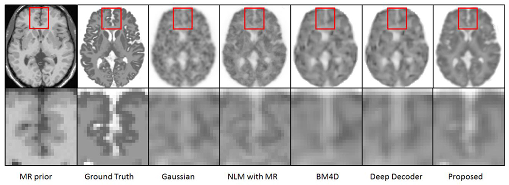
The denoised images using different methods with different parameters (Gaussian: FWHM=2.5 pixels; NLM: widow size 5×5×5; BM4D: noise standard deviation 50 percentage; Deep Decoder: 3800 epochs; the proposed method: 200 epochs) for the simulated brain dataset. The first column is the corresponding MR prior image.

Figure 3.

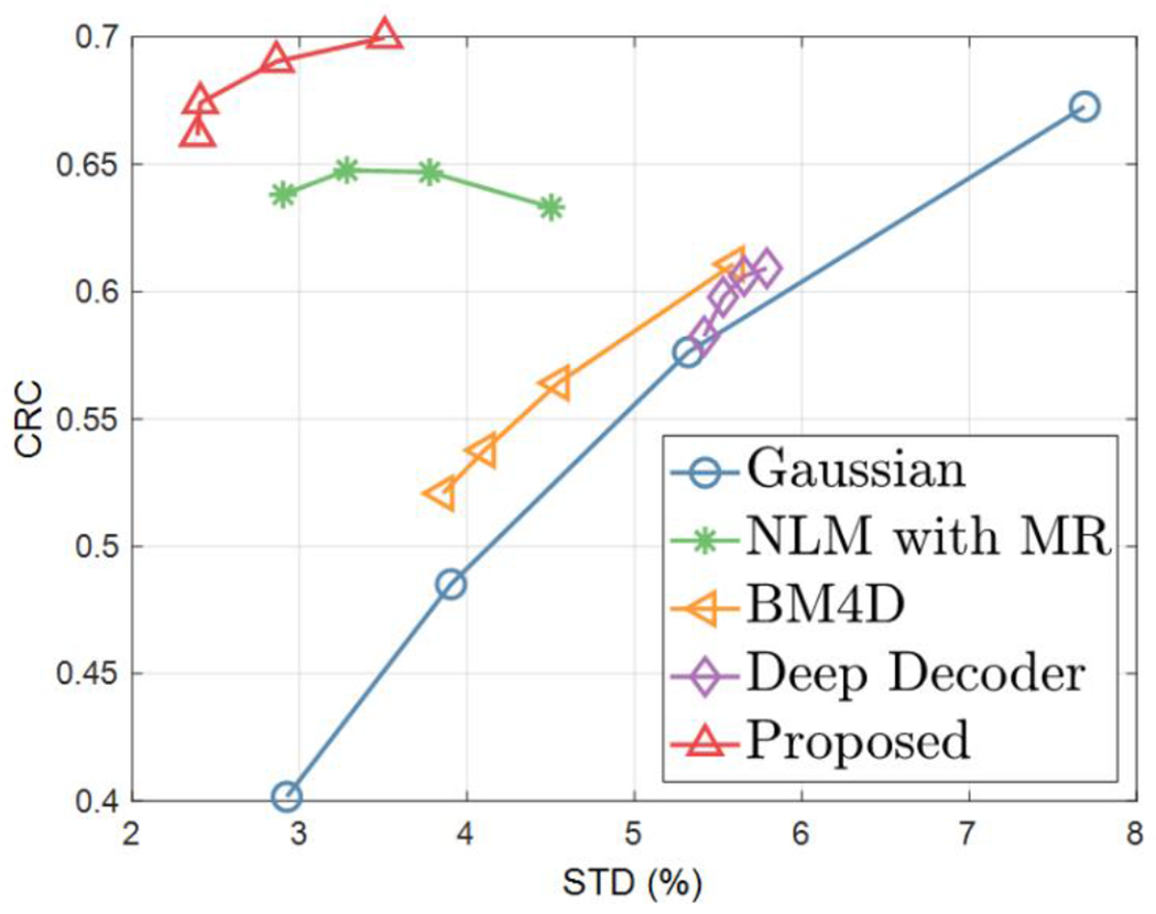
The CRC-STD curves, between the gray matter region and the white matter region for the simulation study. Markers are generated for different FWHM (1.5, 2.5, 3.5, 4.5 pixels) of Gaussian, different window size (5, 7, 9, 11 pixels) of NLM, different noise standard deviation (40, 50, 60, 70 percentages) of BM4D, different epochs (2000, 2600, 3200, 3800) of Deep Decoder and different epochs (150, 200, 220, 250) of the proposed method.

PET/CT

Fig. 4 shows one coronal view of the PET images processed using different methods. In this figure, the parameters for each method were set by maximizing the CNR. Based on the image appearance, we can see that the proposed method can generate images with preserved tumor structures (indicated by arrows) and less noise, while the smoothing effects of all the other methods reduce tumor uptakes. Detailed CNR values and CNR improvement ratios for all ten patient datasets are listed in supplementary Table. 3. The mean (±SD) CNR for the original PET images is 13.04 ± 6.30. The mean (±SD) CNRs for Gaussian, NLM, BM4D, Deep Decoder and the proposed method are 14.62 ± 6.85, 15.94 ± 7.47, 18.28 ± 9.68, 18.80 ±10.10 and 20.35 ± 10.72, respectively. Fig. 5 shows the bar plot of CNR improvement ratios for all ten datasets using different methods. The overall performance of the proposed method (orange) is higher than Gaussian (gray), NLM with CT (blue), BM4D (yellow) and Deep Decoder (green), especially for patient 7 and 10, where its CNR improvement ratio are much better than other methods. The mean (±SD) CNR improvement ratios for Gaussian, NLM, BM4D, Deep Decoder and the proposed method are 12.64% ± 6.15%, 24.35% ± 16.30%, 38.31% ± 20.26%, 41.67% ± 22.28% and 53.35% ± 21.78%, respectively. Fig.8 shows the box plot of CNR improvement ratios using different methods. We can see that the CNR improvement ratio of the proposed method is significantly higher than the Gaussian (P=0.002), NLM (P=0.002), BM4D (P=0.002) and Deep Decoder (P=0.002) methods.

Figure 4.

Coronal view of (a) the original noisy PET image; (b) the post-processed PET image using the Gaussian filter with FWHM = 2.4 pixel; (c) the post-processed PET image using the NLM filter guided by CT using window size 5×5×5; (d) the post-processed PET image using the BM4D method with 10 percent noise standard deviation; (e) the post-processed PET image using the Deep Decoder method with 1800 epochs; (f) the post-processed PET image using the proposed method trained with 900 epochs. Tumors are pointed out using arrows.

Figure 5.

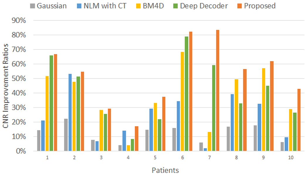
The CNR improvement ratios of ten PET/CT datasets using the Gaussian, NLM guided by CT, BM4D, Deep Decoder and the proposed method.

Figure 8.

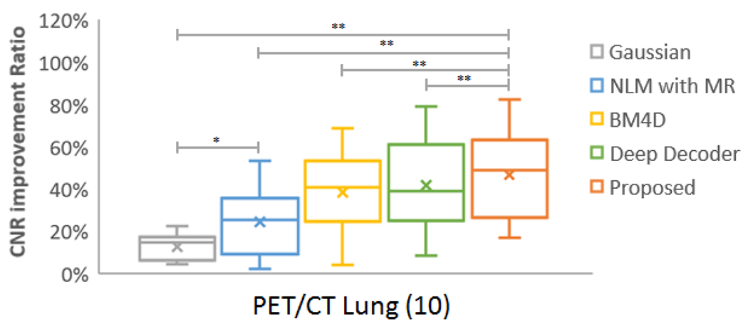
Box plot of CNR improvement ratios for 10 lung tumor patients in PET/CT datasets. In the boxplots, lines indicating median, 25th and 75th percentiles; cross displaying the mean value; * and ** representing P<0.05 and P<0.01, respectively.

PET/MR

Fig. 6 presents one coronal view of the PET images processed by the Gaussian, NLM guided by MR, BM4D, Deep Decoder and the proposed method, given the optimum parameters regarding the CNR. For the tumor regions, we can see that the proposed method preserves the tumor uptake. Zoomed subfigures show that the proposed method can recover the cardiac and spleen structures better than other methods. The CNR values and CNR improvement ratios calculated for all 30 patients are shown in supplementary Table 4. The mean (±SD) CNR for the original PET images is 39.34 ± 27.81. The mean (±SD) CNRs for the Gaussian, NLM, BM4D, Deep Decoder and the proposed method are 46.42 ± 33.94, 49.17 ± 36.82, 54.15 ± 39.32, 52.18 ± 39.63 and 58.35 ± 43.18, respectively. The mean (±SD) CNR improvement ratios for the Gaussian, NLM, BM4D, Deep Decoder and the proposed method are 18.16% ± 10.02%, 25.36% ± 19.48%, 37.02% ±21.38%, 30.03% ± 20.64% and 46.80% ± 25.23%, respectively. Bar plot in Fig. 7 shows the CNR improvement ratios for all the 30 patients. For the whole PET/MR data set, CNR improvement ratio of the proposed method is significantly higher than the Gaussian (P<0.0001), NLM (P<0.0001), BM4D (P<0.0001) and Deep Decoder (P<0.0001) methods. CNR improvement ratios for different tumor types were further analyzed, and the box plots of tumor types with more than five specimens (liver: 12, lung:6) are listed in Fig. 9. For liver and lung tumors, the mean (±SD) CNR improvement ratios of the proposed method (liver: 43.37% ± 30.85%; lung: 35.91% ± 10.48%) are significantly higher than the Gaussian (liver: 18.80% ± 9.98%, P<0.001; lung: 13.20% ± 5.44%, P<0.05), NLM (liver: 28.00% ± 21.97%, P<0.001; lung: 15.65% ± 8.56%, P<0.05), BM4D (liver: 36.13% ± 26.80%, P<0.001; lung: 27.32% ± 9.66%, P<0.05), and Deep Decoder (liver:29.19% ±24.73%, P<0.001; lung: 17.80% ± 11.30%, P<0.05) methods.

Figure 6.

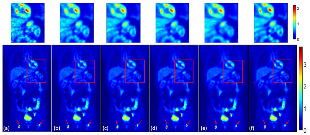
Coronal view of (a) the original noisy PET image; (b) the post-processed image using the Gaussian filter with FWHM = 1.6 pixel; (c) the post-processed image using the NLM filter guided by MR with window size 5×5×5; (d) the post-processed PET image using the BM4D method with 8 percent noise standard deviation; (e) the post-processed PET image using the Deep Decoder method with 2000 epochs; (f) the post-processed PET image using the proposed method trained with 700 epochs. Tumors are pointed out using arrows. Details in the red box are zoomed-in and shown above the whole-body images using a different color bar with the maximum value of 2.2.

Figure 7.

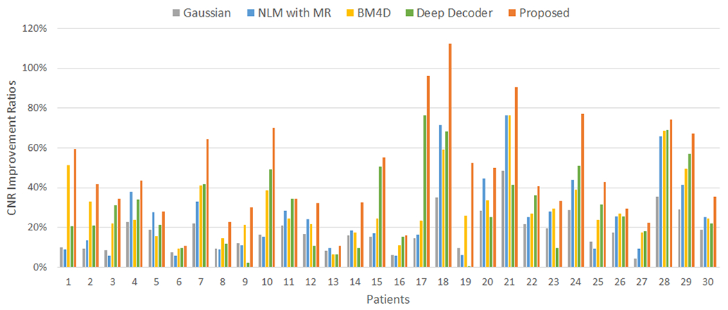
The CNR improve ratios of thirty PET/MR datasets using the Gaussian, NLM guided by MR, BM4D, Deep Decoder and the proposed method.

Figure 9.

Box plot of CNR improvement ratios for different tumor types in PET/MR datasets. Number of patients for each tumor type is listed in the bracket. In the boxplots, lines indicating median, 25^th and 75^th percentiles; cross displaying the mean value; *, *** and ns representing P<0.05, P<0.001 and nonsignificant, respectively.

DISCUSSION

The plot of the contrast (m_lesion − m_ref) vs. noise inside reference ROIs (SD_ref) for different methods with varying parameters (supplementary Fig. 4) shows that the proposed method can maintain high contrast within the tumor region while achieving low noise in the reference region. Compared to the proposed method, the NLM method could not preserve high contrast with the same noise and the Gaussian method showed higher noise at the same contrast level. From Fig. 9 we can see that there is no significant difference between the Gaussian method and the MR-guided NLM method for the lung tumor. The fact that the T1-weighted image does not have too many details in the lung region might be one explanation. However, the proposed method using MR as prior can still achieve significantly higher CNR improvement ratio compared with the Gaussian and NLM methods for the lung tumor case, which demonstrates that the proposed method can make use of priors more efficiently than the NLM method.

Apart from comparing the proposed method with state-of-the-arts methods, we are also interested in understanding the factors influencing its performance. Influence of the following factors were evaluated for the proposed method: modality of prior images, PET tracer types, tumor sizes and tumor uptakes. For the dataset of PET/CT with ⁶⁸Ga-PRGD2 and the dataset of PET/MR with ¹⁸F-FDG, the mean (± SD) improvement ratios (53.35% ± 21.78%, 46.80% ± 25.23%) are approximately the same and there is no significant difference, which shows that the proposed denoising method works well regardless of modality types and tracer types used in this work. The tumor size, SUV_max, SUV_mean and total lesion glycolysis (TLG) versus CNR improvement ratio for the two datasets are plotted in supplementary Fig. 5. Here TLG is the product of tumor size and SUV_mean, which can show joint effects of tumor size and tracer uptake. We can see that there is no clear correlation of tumor size, SUV_max, SUV_mean, and TLG with CNR improvement ratio, which is further verified by the correlation coefficients presented in Table 1. This tells us that the proposed denoising method is robust for various tumor sizes and tumor uptakes. In addition, supplementary Fig. 6 is an example showing that even when there are some mismatches in the tumor structure between the PET image and its corresponding CT image, the proposed method can still recover the tumor structure, which verifies that misregistration might not lead to artefacts or local distortions of the proposed method. Further investigations regarding the detailed effects of misregistration on the proposed method are needed and are our future work.

Table 1.

The correlations of CNR values and CNR improvement ratios with different tumor features for all scans of PET/CT and PET/MR datasets.

Correlation		tumor size	SUV max	SUV mean	TLG
PET/CT	Improvement ratio	0.3734	0.3409	0.1286	0.3664
	CNR	−0.0407	0.8949(p<0.05)	0.8192(p<0.05)	0.1909
PET/MR	Improvement ratio	0.1821	0.0039	−0.0601	0.1039
	CNR	0.3251	0.8483(p<0.0001)	0.8508(p<0.0001)	0.6475(p<0.0001)

CONCLUSION

In this work, we proposed an unsupervised deep learning method for PET denoising, where the patient’s prior image was employed as the network input and the original noisy PET image was treated as the training label. Evaluations based on simulation datasets as well as PET/CT and PET/MR datasets demonstrate the effectiveness of the proposed denoising method over the Gaussian, anatomically guided NLM, BM4D and Deep Decoder methods. Future work will focus on further clinical evaluations with various tumor types as well as the detailed effects of misregistration on the proposed method.

References

- 1.Fletcher JW, Djulbegovic B, Soares HP, Siegel BA, Lowe VJ, Lyman GH, et al. Recommendations on the Use of 18F-FDG PET in Oncology. J Nucl Med [Internet] 2008;49:480–508. Available from: 10.2967/jnumed.107.047787 [DOI] [PubMed] [Google Scholar]
- 2.Beyer T, Townsend DW, Brun T, Kinahan PE, Charron M, Roddy R, et al. A combined PET/CT scanner for clinical oncology. J Nucl Med. 2000;41:1369–79. [PubMed] [Google Scholar]
- 3.Schwaiger M, Ziegler S, Nekolla SG. PET/CT: challenge for nuclear cardiology. J Nucl Med. 2005;46:1664–78. [PubMed] [Google Scholar]
- 4.Tai YF. Applications of positron emission tomography (PET) in neurology. J Neurol Neurosurg Psychiatry [Internet] 2004;75:669–76. Available from: 10.1136/jnnp.2003.028175 [DOI] [PMC free article] [PubMed] [Google Scholar]
- 5.Gong K, Majewski S, Kinahan PE, Harrison RL, Elston BF, Manjeshwar R, et al. Designing a compact high performance brain PET scanner - Simulation study Phys Med Biol. IOP Publishing; 2016;61:3681–97. Available from: 10.1088/0031-9155/61/10/3681 [DOI] [PMC free article] [PubMed] [Google Scholar]
- 6.Tauber C, Stute S, Chau M, Spiteri P, Chalon S, Guilloteau D, et al. Spatio-temporal diffusion of dynamic PET images. Phys Med Biol. 2011;56:6583–96. Available from: 10.1088/0031-9155/56/20/004 [DOI] [PubMed] [Google Scholar]
- 7.Dutta J, Leahy RM, Li Q. Non-Local Means Denoising of Dynamic PET Images Muñoz-Barrutia A, editor. PLoS One [Internet] 2013;8:e81390 Available from: 10.1371/journal.pone.0081390 [DOI] [PMC free article] [PubMed] [Google Scholar]
- 8.Boussion N, Cheze Le Rest C, Hatt M, Visvikis D. Incorporation of wavelet-based denoising in iterative deconvolution for partial volume correction in whole-body PET imaging. Eur J Nucl Med Mol Imaging. 2009;36:1064–75. Available from: 10.1007/s00259-009-1065-5 [DOI] [PubMed] [Google Scholar]
- 9.Shidahara M, Ikoma Y, Seki C, Fujimura Y, Naganawa M, Ito H, et al. Wavelet denoising for voxel-based compartmental analysis of peripheral benzodiazepine receptors with 18F-FEDAA1106. Eur J Nucl Med Mol Imaging. 2008;35:416–23. Available from: 10.1007/s00259-007-0623-y [DOI] [PubMed] [Google Scholar]
- 10.Christian BT, Vandehey NT, Floberg JM, Mistretta CA. Dynamic PET Denoising with HYPR Processing. J Nucl Med [Internet] 2010;51:1147–54. Available from: 10.2967/jnumed.109.073999 [DOI] [PMC free article] [PubMed] [Google Scholar]
- 11.Xu Z, Bagci U, Seidel J, Thomasson D, Solomon J, Mollura DJ. Segmentation based denoising of PET images: an iterative approach via regional means and affinity propagation. Med Image Comput Comput Assist Interv [Internet] 2014;17:698–705. Available from: 10.1007/978-3-319-10404-1_87 [DOI] [PMC free article] [PubMed] [Google Scholar]
- 12.Comtat C, Kinahan PE, Fessler JA, Beyer T, Townsend DW, Defrise M, et al. Clinically feasible reconstruction of 3D whole-body PET/CT data using blurred anatomical labels. Phys Med Biol. 2002;47:1–20. Available from: 10.1088/0031-9155/47/1/301 [DOI] [PubMed] [Google Scholar]
- 13.Baete K, Nuyts J, Van Paesschen W, Suetens P, Dupont P. Anatomical-Based FDG-PET Reconstruction for the Detection of Hypo-Metabolic Regions in Epilepsy. IEEE Trans Med Imaging [Internet] 2004;23:510–9. Available from: 10.1109/tmi.2004.825623 [DOI] [PubMed] [Google Scholar]
- 14.Bowsher JE, Yuan Hong, Hedlund LW, Turkington TG, Akabani G, Badea A, et al. Utilizing MRI Information to Estimate F18-FDG Distributions in Rat Flank Tumors. IEEE Symp Conf Rec Nucl Sci 2004 IEEE; 2004. p. 2488–92. Available from: 10.1109/nssmic.2004.1462760 [DOI] [Google Scholar]
- 15.Chan C, Fulton R, Barnett R, Feng DD, Meikle S. Postreconstruction Nonlocal Means Filtering of Whole-Body PET with an Anatomical Prior. IEEE Trans Med Imaging. 2014;33:636–50. Available from: 10.1109/tmi.2013.2292881 [DOI] [PubMed] [Google Scholar]
- 16.Yan J, Lim JCS, Townsend DW. MRI-guided brain PET image filtering and partial volume correction Phys Med Biol. IOP Publishing; 2015;60:961–76. Available from: 10.1109/nssmic.2013.6829058 [DOI] [PubMed] [Google Scholar]
- 17.He K, Sun J, Tang X. Guided Image Filtering. IEEE Trans Pattern Anal Mach Intell. 2013;35:1397–409. [DOI] [PubMed] [Google Scholar]
- 18.Somayajula S, Panagiotou C, Rangarajan A, Li Q, Arridge SR, Leahy RM. PET Image Reconstruction Using Information Theoretic Anatomical Priors. IEEE Trans Med Imaging. 2011;30:537–49. Available from: 10.1109/nssmic.2005.1596899 [DOI] [PMC free article] [PubMed] [Google Scholar]
- 19.Tang J, Rahmim A. Bayesian PET image reconstruction incorporating anato-functional joint entropy. Phys Med Biol. 2009;54:7063–75. Available from: 10.1109/isbi.2008.4541178 [DOI] [PMC free article] [PubMed] [Google Scholar]
- 20.Nuyts J The use of mutual information and joint entropy for anatomical priors in emission tomography. 2007 IEEE Nucl Sci Symp Conf Rec IEEE; 2007. p. 4149–54. Available from: 10.1109/nssmic.2007.4437034 [DOI] [Google Scholar]
- 21.Song T, Yang F, Chowdhury SR, Kim K, Johnson KA, Fakhri G El, et al. PET Image Deblurring and Super-Resolution with an MR-Based Joint Entropy Prior. IEEE Trans Comput Imaging. 2019;1 Available from: 10.1109/tci.2019.2913287 [DOI] [PMC free article] [PubMed] [Google Scholar]
- 22.Wang S, Su Z, Ying L, Peng X, Zhu S, Liang F, et al. Accelerating magnetic resonance imaging via deep learning. 2016 IEEE 13th Int Symp Biomed Imaging IEEE; 2016. p. 514–7. Available from: 10.1109/isbi.2016.7493320 [DOI] [PMC free article] [PubMed] [Google Scholar]
- 23.Chen H, Zhang Y, Zhang W, Liao P, Li K, Zhou J, et al. Low-dose CT via convolutional neural network. Biomed Opt Express. 2017;8:679. [DOI] [PMC free article] [PubMed] [Google Scholar]
- 24.Wu D, Kim K, Fakhri G El, Li Q. A Cascaded Convolutional Neural Network for X-ray Low-dose CT Image Denoising. 2017; [Google Scholar]
- 25.Gong K, Guan J, Kim K, Zhang X, Yang J, Seo Y, et al. Iterative PET Image Reconstruction Using Convolutional Neural Network Representation. IEEE Trans Med Imaging. 2018;1–8. Available from: 10.1109/tmi.2018.2869871 [DOI] [PMC free article] [PubMed] [Google Scholar]
- 26.Chen KT, Gong E, de Carvalho Macruz FB, Xu J, Boumis A, Khalighi M, et al. Ultra–Low-Dose 18 F-Florbetaben Amyloid PET Imaging Using Deep Learning with Multi-Contrast MRI Inputs. Radiology. 2019;290:649–56. Available from: 10.1148/radiol.2018180940 [DOI] [PMC free article] [PubMed] [Google Scholar]
- 27.Xiang L, Qiao Y, Nie D, An L, Wang Q, Shen D. Deep Auto-context Convolutional Neural Networks for Standard-Dose PET Image Estimation from Low-Dose PET/MRI. Neurocomputing. 2018;406–16. Available from: 10.1016/j.neucom.2017.06.048 [DOI] [PMC free article] [PubMed] [Google Scholar]
- 28.Ulyanov D, Vedaldi A, Lempitsky V. Deep Image Prior. 2017 IEEE Conf Comput Vis Pattern Recognit IEEE; 2017;5882–91. Available from: 10.1109/cvpr.2018.00984 [DOI] [Google Scholar]
- 29.Mirza M, Osindero S. Conditional Generative Adversarial Nets. Cambridge: Cambridge University Press; 2014;1–7. Available from: http://arxiv.org/abs/1411.1784 [Google Scholar]
- 30.Çiçek Ö, Abdulkadir A, Lienkamp SS, Brox T, Ronneberger O. 3D U-Net: Learning Dense Volumetric Segmentation from Sparse Annotation. Lect Notes Comput Sci (including Subser Lect Notes Artif Intell Lect Notes Bioinformatics) [Internet] 2016. p. 424–32. Available from: 10.1007/978-3-319-46723-8_49 [DOI] [Google Scholar]
- 31.Gong K, Kim K, Cui J, Guo N, Catana C, Qi J, et al. Learning Personalized Representation for Inverse Problems in Medical Imaging Using Deep Neural Network. 2018;1–11. Available from: http://arxiv.org/abs/1807.01759
- 32.Liu DC, Nocedal J. On the limited memory BFGS method for large scale optimization. Math Program [Internet] 1989;45:503–28. Available from: 10.1007/bf01589116 [DOI] [Google Scholar]
- 33.Kingma DP, Ba J. Adam: A Method for Stochastic Optimization. 2014; Available from: http://arxiv.org/abs/1412.6980
- 34.NESTEROV Y A method for unconstrained convex minimization problem with the rate of convergence o(1/k^2). Dokl AN USSR [Internet] 1983;269:543–7. [Google Scholar]
- 35.Cocosco CA, Kollokian V, Kwan RK-S, Pike GB, Evans AC. Brainweb: Online interface to a 3D MRI simulated brain database. Neuroimage. Citeseer; 1997. [Google Scholar]
- 36.Maggioni M, Katkovnik V, Egiazarian K, Foi A. Nonlocal Transform-Domain Filter for Volumetric Data Denoising and Reconstruction. IEEE Trans Image Process [Internet] 2013;22:119–33. Available from: 10.1109/tip.2012.2210725 [DOI] [PubMed] [Google Scholar]
- 37.Heckel R, Hand P. Deep Decoder: Concise Image Representations from Untrained Non-convolutional Networks. Int Conf Learn Represent [Internet] International Conference on Learning Representations; 2019. Available from: 10.1109/TIP.2012.2210725 [DOI] [Google Scholar]
Associated Data
This section collects any data citations, data availability statements, or supplementary materials included in this article.