Modeling and forecasting the spread of COVID-19 with stochastic and deterministic approaches: Africa and Europe

Abstract

Using the existing collected data from European and African countries, we present a statistical analysis of forecast of the future number of daily deaths and infections up to 10 September 2020. We presented numerous statistical analyses of collected data from both continents using numerous existing statistical theories. Our predictions show the possibility of the second wave of spread in Europe in the worse scenario and an exponential growth in the number of infections in Africa. The projection of statistical analysis leads us to introducing an extended version of the well-blancmange function to further capture the spread with fractal properties. A mathematical model depicting the spread with nine sub-classes is considered, first converted to a stochastic system, where the existence and uniqueness are presented. Then the model is extended to the concept of nonlocal operators; due to nonlinearity, a modified numerical scheme is suggested and used to present numerical simulations. The suggested mathematical model is able to predict two to three waves of the spread in the near future.

Introduction

Interdisciplinary research is the way forward for mankind to be in control of its environment. Of course they will not be able to have total control since the nature within which they live is full of uncertainties, many complex phenomena that have not been yet understood with the current collections of knowledge and technology. For example, we cannot explicitly and confidently explain what is happening at the Bermuda Triangle, although many studies have been done around this place, some believe it is a devil’s triangle. There are many other natural occurrences that could not be explained so far with our knowledge. But it has been proven that putting together several concepts from different academic fields could provide better results. COVID-19 is an invisible enemy that left humans with no choice than to put all their efforts from all backgrounds with the aim to protect the survival of their kind. Many souls have been taken, many humans have been infected and some recovered, but still the spread has not yet reached its peak in many countries. While in some countries the curve of daily new infected has nearly reached zero, in others the spread is increasing exponentially. For some statistical analysis, we investigated daily cases of infections and deaths due to the COVID-19 spread that occurred in 54 countries in the European continent and 47 countries in the African continent from the beginning of the outbreak to 15 June 2020. To do this, we used the available data on the website of the World Health Organization (WHO) [1, 2]. Although mathematicians cannot provide vaccine or cure the disease in an infected person, they can use their mathematical tools to foresee what could possibly happen in the near future with some limitations [3–14]. With the new trend of spread, it is possible that the world will face a second wave of COVID-19 spread, this will be the aim of our work.

The paper is organized as follows. In Sect. 2, we present the definitions of differential and integral operators where singular and nonsingular kernels are used. In Sect. 3, the parameter estimations are presented for the infected and deaths in Africa and Europe using the Box–Jenkins model. In Sect. 4, the simulations for smoothing method for the infected and deaths in Africa and Europe are presented. In Sect. 5, the predictions about the cases of infections and deaths in Africa and Europe are provided. In Sect. 6, we give an analysis of COVID-19 spread based on fractal interpolation and fractal dimension. In Sect. 7, existence and uniqueness for a mathematical model with stochastic component are investigated. Also the numerical simulations for such a model are depicted. In Sect. 8, we present a modified scheme based on the Newton polynomial. In Sect. 9, we provide numerical solutions for the suggested COVID-19 model with different differential operators.

Differential and integral operators

In this section, we present some definitions of differential and integral operators with singular and nonsingular kernels. The fractional derivatives with power-law, exponential decay, and Mittag-Leffler kernel are given as follows:

Definition 1

$$\begin{array}{c}{}_0{}^{C}D_t^{\alpha }f(t)=\frac{1}{\mathrm{\Gamma }(1-\alpha )}{\int }_0^t\frac{d}{d\tau }f(\tau ){(t-\tau )}^{-\alpha }d\tau ,\hfill \\ {}_0{}^{CF}D_t^{\alpha }f(t)=\frac{M(\alpha )}{1-\alpha }{\int }_0^t\frac{d}{d\tau }f(\tau )exp[-\frac{\alpha }{1-\alpha }(t-\tau )]d\tau ,\hfill \\ {}_0{}^{ABC}D_t^{\alpha }f(t)=\frac{AB(\alpha )}{1-\alpha }{\int }_0^t\frac{d}{d\tau }f(\tau )E_{\alpha }[-\frac{\alpha }{1-\alpha }{(t-\tau )}^{\alpha }]d\tau .\hfill \end{array}$$ 1

The fractional integrals with power-law, exponential decay, and Mittag-Leffler kernel are given as follows:

$$\begin{array}{c}{}_0{}^{C}J_t^{\alpha }f(t)=\frac{1}{\mathrm{\Gamma }(\alpha )}{\int }_0^t{(t-\tau )}^{\alpha -1}f(\tau )d\tau ,\hfill \\ {}_0{}^{CF}J_t^{\alpha ,\beta }f(t)=\frac{1-\alpha }{M(\alpha )}f(t)+\frac{\alpha }{M(\alpha )}{\int }_0^{t}f(\tau )d\tau ,\hfill \\ {}_0{}^{AB}J_t^{\alpha ,\beta }f(t)=\frac{1-\alpha }{AB(\alpha )}f(t)+\frac{\alpha }{AB(\alpha )\mathrm{\Gamma }(\alpha )}{\int }_0^t{(t-\tau )}^{\alpha -1}f(\tau )d\tau .\hfill \end{array}$$ 2

The fractal-fractional derivatives with power-law kernel, exponential decay, and Mittag-Leffler kernel are given as follows:

$$\begin{array}{c}{}_0{}^{FFP}D_t^{\alpha ,\beta }f(t)=\frac{1}{\mathrm{\Gamma }(1-\alpha )}\frac{d}{d{t}^{\beta }}{\int }_0^{t}f(\tau ){(t-\tau )}^{-\alpha }d\tau ,\hfill \\ {}_0{}^{FFE}D_t^{\alpha ,\beta }f(t)=\frac{M(\alpha )}{1-\alpha }\frac{d}{d{t}^{\beta }}{\int }_0^{t}f(\tau )exp[-\frac{\alpha }{1-\alpha }(t-\tau )]d\tau ,\hfill \\ {}_0{}^{FFM}D_t^{\alpha ,\beta }f(t)=\frac{AB(\alpha )}{1-\alpha }\frac{d}{d{t}^{\beta }}{\int }_0^{t}f(\tau )E_{\alpha }[-\frac{\alpha }{1-\alpha }{(t-\tau )}^{\alpha }]d\tau ,\hfill \end{array}$$ 3

where

$$\frac{df(t)}{d{t}^{\beta }}=\underset{t\to t_1}{lim}\frac{f(t)-f(t_1)}{t^{2-\beta }-t_1^{2-\beta }}(2-\beta ).$$ 4

The fractal-fractional integrals with power-law, exponential decay, and Mittag-Leffler kernel are as follows:

$$\begin{array}{c}{}_0{}^{FFP}J_t^{\alpha ,\beta }f(t)=\frac{1}{\mathrm{\Gamma }(\alpha )}{\int }_0^t{(t-\tau )}^{\alpha -1}{\tau }^{1-\beta }f(\tau )d\tau ,\hfill \\ {}_0{}^{FFE}J_t^{\alpha ,\beta }f(t)=\frac{1-\alpha }{M(\alpha )}{t}^{1-\beta }f(t)+\frac{\alpha }{M(\alpha )}{\int }_0^t{\tau }^{1-\beta }f(\tau )d\tau ,\hfill \\ {}_0{}^{FFM}J_t^{\alpha ,\beta }f(t)=\frac{1-\alpha }{AB(\alpha )}{t}^{1-\beta }f(t)+\frac{\alpha }{AB(\alpha )\mathrm{\Gamma }(\alpha )}{\int }_0^t{(t-\tau )}^{\alpha -1}{\tau }^{1-\beta }f(\tau )d\tau .\hfill \end{array}$$ 5

Box–Jenkin’s model development

Autoregressive integrated moving average (ARIMA) approach suggested by Box and Jenkins is one of the most powerful techniques used in time series analysis. The ARIMA model is composed of three parts. First, the autoregressive part is a linear regression which has a relation between past values and future values of data series; second, the integrated part expresses how many times the data series has to be differenced to obtain a stationary series; and the last one is the moving average part which has a relation between past forecast errors and future values of data series [14]. These processes can be presented by the models $AR(p)$, $MA(q)$, $ARMA(p,q)$, and $ARIMA(p,d,q)$. We should decide which model we will choose for our data series. To do this, partial autocorrelation (PACF) and the autocorrelation (ACF) are helpful to obtain parameters for the AR model and the MA model, respectively.

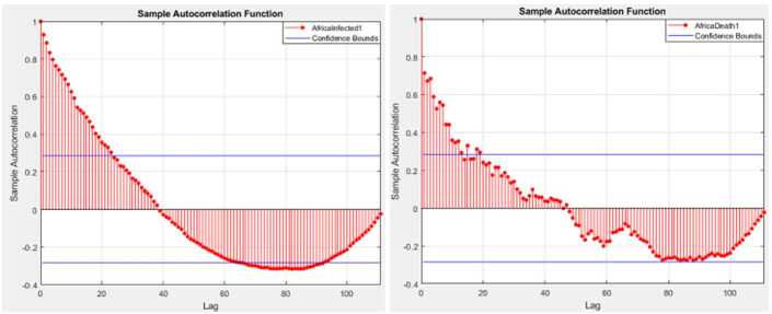
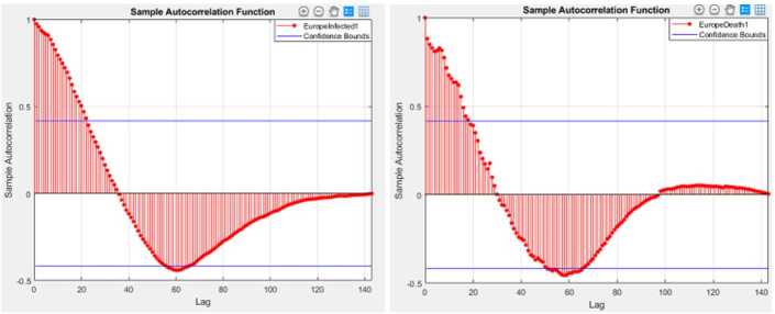
Figures 1 and 2 depict graphs of autocorrelation functions for the infected and deaths in Africa and Europe.

Figure 1.

Autocorrelation function for the infected and deaths in Africa

Figure 2.

Autocorrelation function for the infected and deaths in Europe

Now we introduce these models. Let $Y_t$ be the value of the time series at time t. Time series as a p-order autoregressive process is as follows:

$$Y_t=\delta +{\phi }_1{Y}_{t-1}+{\phi }_2{Y}_{t-2}+\cdots +{\phi }_p{Y}_{t-p}+{\epsilon }_t,$$ 6

which is shown as $AR(p)$. Here, δ and ${\epsilon }_t$ describe constant and error terms, respectively. Time series as a qth degree of moving average process is given by

$$Y_t=\mu +{\epsilon }_t+{\theta }_1{\epsilon }_{t-1}+{\theta }_2{\epsilon }_{t-2}+\cdots +{\theta }_q{\epsilon }_{t-q},$$ 7

which is shown as $MA(q)$. The $ARMA(p,q)$ expression is obtained as a combination of $AR(p)$ and $MA(q)$ equations:

$$Y_t=\delta +{\phi }_1{Y}_{t-1}+{\phi }_2{Y}_{t-2}+\cdots +{\phi }_p{Y}_{t-p}+{\epsilon }_t+{\theta }_1{\epsilon }_{t-1}+{\theta }_2{\epsilon }_{t-2}+\cdots +{\theta }_q{\epsilon }_{t-q}.$$ 8

When the time series is not stationary, we take the difference d times to make it stationary. The $ARIMA(p,q)$ model is given by

$$(1-{\phi }_{1}l-{\phi }_2{l}^2-\cdots -{\phi }_p{l}^p){\mathrm{\Delta }}^d{Y}_t=\delta +{\epsilon }_t+{\theta }_1{\epsilon }_{t-1}+{\theta }_2{\epsilon }_{t-2}+\cdots +{\theta }_q{\epsilon }_{t-q}.$$ 9

In the ARIMA technique, the model performance can be measured by using some criteria, for instance, Akaike information criteria(AIC), Bayesian information criteria(BIC). Here, we benefit from the Akaike information criteria given as follows:

$$\begin{array}{c}AIC=-2log(l)+2k,\hfill \\ BIC=-2log(l)+klnn,\hfill \end{array}$$ 10

where l states likelihood of the data, n is the number of data points, and k also defines the intercept of the ARIMA model. The numerical simulation are depicted in Figs. 3, 4, 5 and 6.

Figure 3.

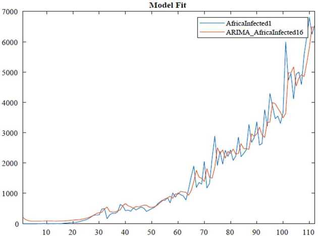
ARIMA model for the infected in Africa

Figure 4.

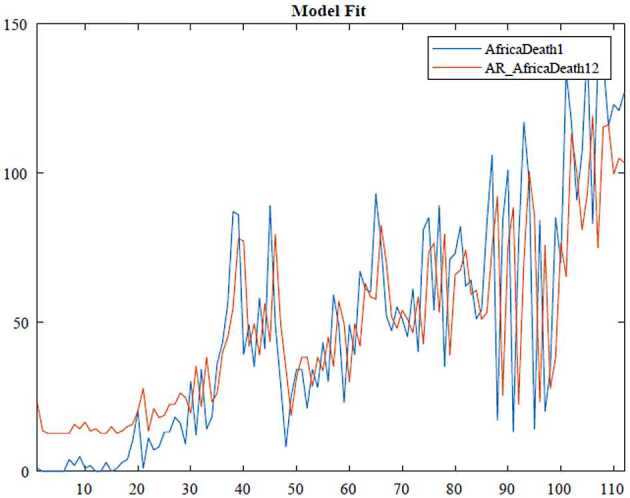
AR model for deaths in Africa

Figure 5.

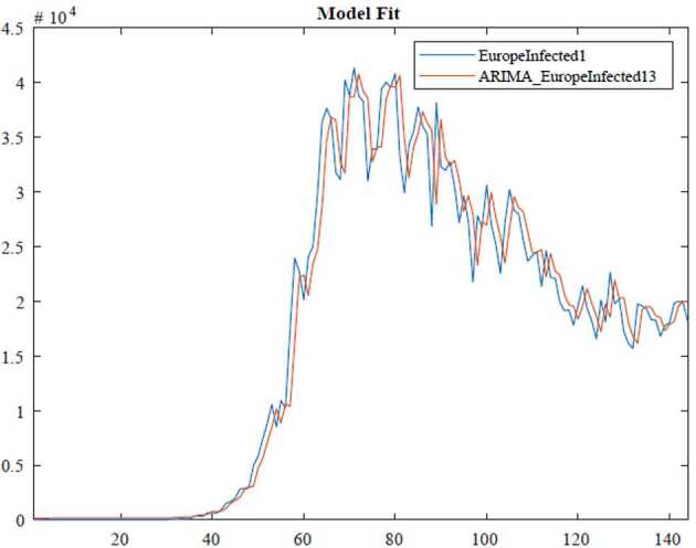
ARIMA model for the infected in Europe

Figure 6.

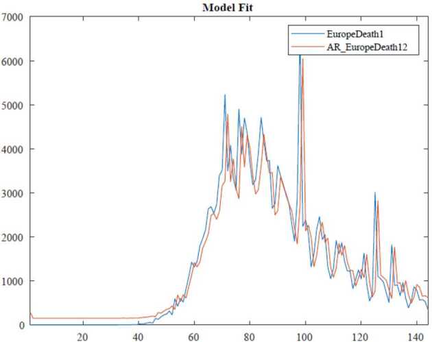
AR model for deaths in Europe

According to data series for the infected in Africa, we use the $ARIMA(2,1,0)$ model which is given by

$$(1-{\phi }_{1}l-{\phi }_2{l}^2)(1-l)Y_t=c+{\epsilon }_t.$$ 11

Here,

$$\begin{array}{c}AIC=1670.1734,\hfill \\ BIC=1680.9388.\hfill \end{array}$$ 12

In Table 1, we give parameter estimation for infections in Africa.

Table 1.

Model estimation for infections in Africa

Parameter	Value	Standard error	TStatistic
Constant	89.2032	56.6511	1.5746
AR{1}	−0.44796	0.099221	−4.5147
AR{2}	−0.17789	0.068294	−2.6047
Variance	168,446.2911	12,738.3089	13.2236

According to data series for deaths in Africa, we use the $AR(1)$ model which is given by

$$(1-{\phi }_{1}l)Y_t=c+{\epsilon }_t.$$ 13

Here,

$$\begin{array}{c}AIC=1056.6482,\hfill \\ BIC=1064.7768.\hfill \end{array}$$ 14

In Table 2, we give parameter estimation for deaths in Africa.

Table 2.

Model estimation for deaths in Africa

Parameter	Value	Standard error	TStatistic
Constant	12.581	6.0023	2.096
AR{1}	0.75094	0.082701	9.0802
Variance	694.3043	92.168	7.533

According to data series for the infected in Europe, we use the $ARIMA(2,1,1)$ model which is given by

$$(1-{\phi }_{1}l-{\phi }_2{l}^2)(1-l)Y_t=c+(1+{\theta }_{1}l){\epsilon }_t.$$ 15

Here,

$$\begin{array}{c}AIC=2690.5358,\hfill \\ BIC=2705.2796.\hfill \end{array}$$ 16

In Table 3, we give parameter estimation for the infected in Europe.

Table 3.

Model estimation for the infected in Europe

Parameter	Value	Standard error	TStatistic
Constant	83.7826	118.7108	0.70577
AR{1}	0.3216	0.59303	0.5423
AR{2}	0.035772	0.16277	0.21977
MA{1}	−0.53222	0.58359	−0.91197
Variance	7,214,609.9182	569,786.6944	12.6619

According to data series for deaths in Europe, we use the $AR(1)$ model which is given by

$$(1-{\phi }_{1}l)Y_t=c+{\epsilon }_t.$$ 17

Here,

$$\begin{array}{c}AIC=1670.1734,\hfill \\ BIC=1680.9388.\hfill \end{array}$$ 18

In Table 4, we give parameter estimation for deaths in Europe.

Table 4.

Model estimation for deaths in Europe

Parameter	Value	Standard error	TStatistic
Constant	151.4852	163.967	0.92388
AR{1}	0.8865	0.041096	21.5714
Variance	460,062.22	27,485.093	16.7386

Brown’s exponential smoothing method

Brown’s linear exponential smoothing is one type of double exponential smoothing based on two different smoothed series. The formula is composed of an extrapolation of a line through the two centers. The Brown exponential smoothing method is helpful to model the time series having trend but no seasonality.

For non-adaptive Brown exponential smoothing, the procedure can be described as follows.

Firstly, we start with the following initialization:

1. $S_0=u_0$,

2. $T_0=u_0$,

3. $a_0=2S_0-T_0$,

4. $F_1=a_0+b_0$.

Then we have the following calculations:

1. $S_t=\alpha u_t+(1-\alpha )S_{t-1}$,

2. $T_t=\alpha S_t+(1-\alpha )T_{t-1}$,

3. $a_t=2S_t+T_{t}63$,

4. $\alpha (S_t-T_t)=(1-\alpha )b_t$,

5. $F_{t+1}=a_t+b_t$,

where $0<\alpha <1$ is the smoothing factor. $S_t$ and $T_t$ are the simply smoothed value and doubly smoothed value for the $(t+1)$th time period, respectively. Also $a_t$ and $b_t$ describe the intercept and the slope, respectively.

In Figs. 7, 8, 9, and 10, we present the simulation for smoothing method for the infected and deaths in Africa and Europe where the smoothing factor was chosen as $\alpha =0.99$.

Figure 7.

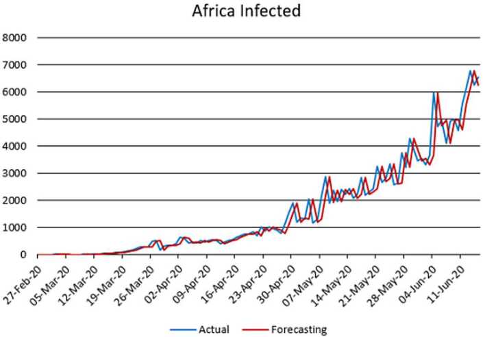
Exponential smoothing for the infected in Africa

Figure 8.

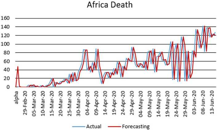
Exponential smoothing for deaths in Africa

Figure 9.

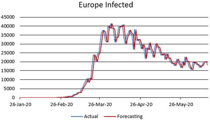
Exponential smoothing for the infected in Europe

Figure 10.

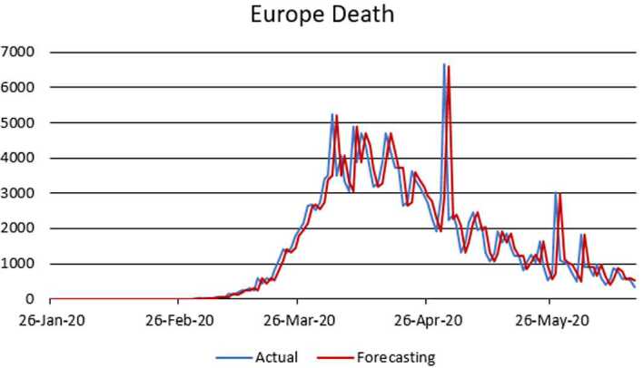
Exponential smoothing for deaths in Europe

Future prediction of daily new numbers of the infected and deaths: Africa and Europe

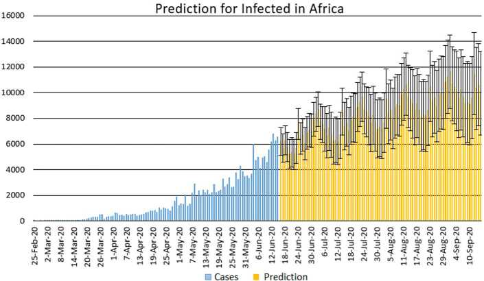
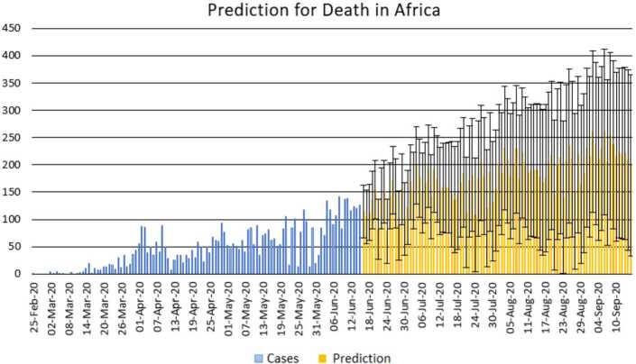
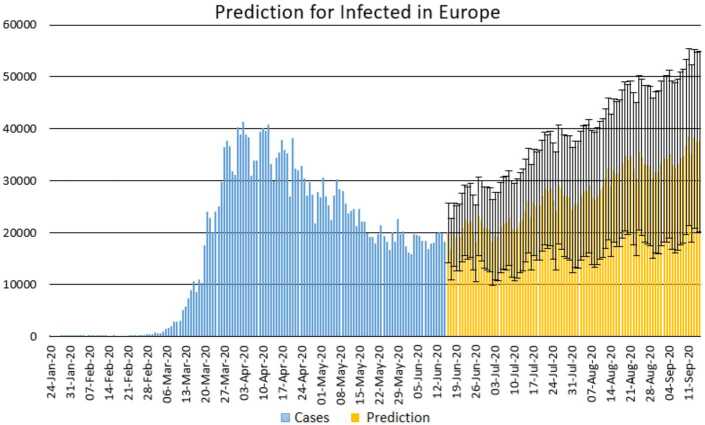
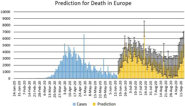
With the collected data using some statistical formula, it is possible to predict what will possibly happen in the near future. Having in mind what could possibly happen, several measures could be taken to avoid the worst case scenario. In this section, with the data collected for 101 countries from Africa (47) and Europe (54), we aim at presenting possible scenarios or events that could be observed in the near future, the daily numbers of deaths and infections. Numerical simulation are presented in Figs. 11, 12, 13 and 14.

Figure 11.

Prediction for the infected in Africa using Forecast Sheet

Figure 12.

Prediction for deaths in Africa using Forecast Sheet

Figure 13.

Prediction for the infected in Europe using Forecast Sheet

Figure 14.

Prediction for deaths in Europe using Forecast Sheet

In Figs. 15, 16, 17, and 18, we present fitting with smoothing spline for the infected and deaths in Africa and Europe.

Figure 15.

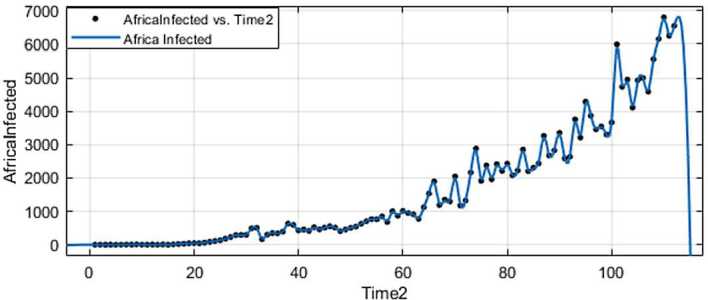
Fitting for the infected in Africa

Figure 16.

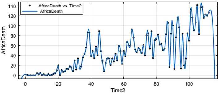
Fitting for deaths in Africa

Figure 17.

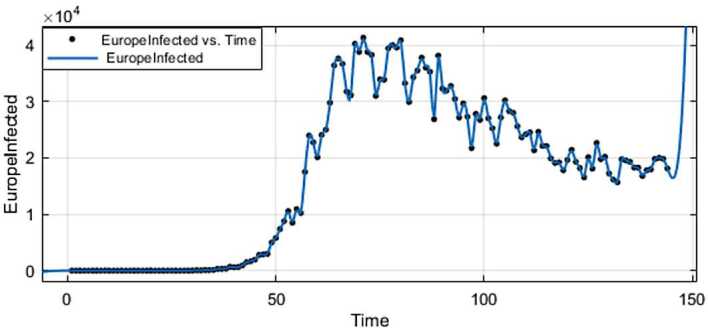
Fitting for the infected in Europe

Figure 18.

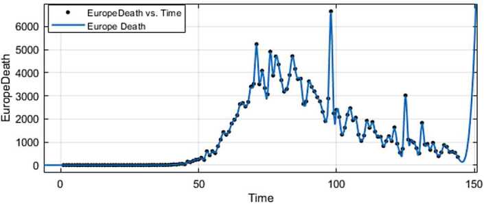
Fitting for deaths in Europe

An analysis of COVID-19 spread based on fractal interpolation and fractal dimension

In this section, we present some information about fractal dimension, interpolation, and blancmange curve.

Fractal dimension

Fractal dimensions enable us to compare fractals. Fractal dimensions are important because they can be defined in connection with real-world data, and they can be measured approximately by means of experiments. These numbers allow us to compare sets in the real world with the laboratory fractals.

Theorem

(The box counting theorem)

Let $N_n(A)$ be the number of boxes of side length $(1/2^n)$. Then the fractal dimension D of A is given as [15]

$$D=\underset{n\to \mathrm{\infty }}{lim}\left\{\frac{ln[N_n(A)]}{ln(2^n)}\right\}.$$ 19

Fractal interpolation

Euclidean geometry and calculus enable us to model using some lines and curves, the shapes that we encounter in the nature [15, 16]. In this section, we present an interpolation function which interpolates the data.

Definition 2

An interpolation function $f:[x_0,x_N]\to \mathbb{R}$ corresponding to the set of data $\{(x_i,F_i)\in {\mathbb{R}}^2:i=0,1,2,\dots ,N\}$ [15]

$$f(x_i)=F_i\text{for }i=1,2,\dots ,N,$$ 20

where $x_0<x_1<x_2\cdots <x_N$.

Let $f:[x_0,x_N]\to \mathbb{R}$ denote the unique continuous function which is called a piecewise linear interpolation function. Also this function is linear on each of the subintervals $[x_{i-1},x_i]$, and it is represented by

$$f(x)=F_{i-1}+\frac{(x-x_{i-1})}{(x_i-x_{i-1})}(F_i-F_{i-1})\text{for }x\in [x_{i-1},x_i],i=1,2,\dots ,N.$$ 21

We have the following transformation, which is iterated:

$$f_n\left(\begin{array}{c}x\\ y\end{array}\right)=\left(\begin{array}{cc}{t}_n& 0\\ u_n& y_n\end{array}\right)\left(\begin{array}{c}x\\ y\end{array}\right)+\left(\begin{array}{c}{v}_n\\ w_n\end{array}\right).$$ 22

When solving this system for $t_n$, $u_n$, $v_n$, and $w_n$ in terms of the data and $y_n$, we obtain the following:

$$\begin{array}{c}{t}_n=\frac{x_n-x_{n-1}}{x_N-x_0},\hfill \\ u_n=\frac{F_n-F_{n-1}}{x_N-x_0}-y_n\frac{F_n-F_0}{x_N-x_0},\hfill \\ v_n=\frac{x_N{x}_{n-1}-x_0{x}_n}{x_N-x_0},\hfill \\ w_n=\frac{x_N{F}_{n-1}-x_0{F}_n}{x_N-x_0}-y_n\frac{x_N{F}_0-x_0{F}_n}{x_N-x_0},\hfill \end{array}$$ 23

where $0\le y_n<1$ is called the scaling factor [15].

Blancmange curve

The blancmange function can be given as an example of fractal interpolation function, and this function is defined by

$$\sum _{n=0}^{\mathrm{\infty }}\frac{S(2^{n}x)}{2^n},x\in [0,1],$$ 24

where $S(x)={min}_{m\in \mathbb{Z}}|x-m|$, $x\in \mathbb{R}$.

However, many problems cannot be depicted when $c=2$ [16]. Then we discuss the limitations of this blancmange; for example, t can only go from 0 to 1, the periodic parameter is 2. Therefore, we change 2 to c, where c is a real number from 1 to a. Therefore, in this section, we extend the blancmange function to a large interval also with any given periodic parameter. So, we have the following formula:

$$\sum _{n=0}^{\mathrm{\infty }}\frac{S(c^{n}x)}{c^n},x\in [0,a],$$ 25

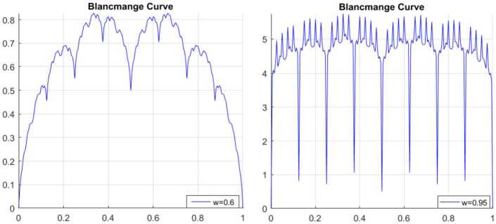
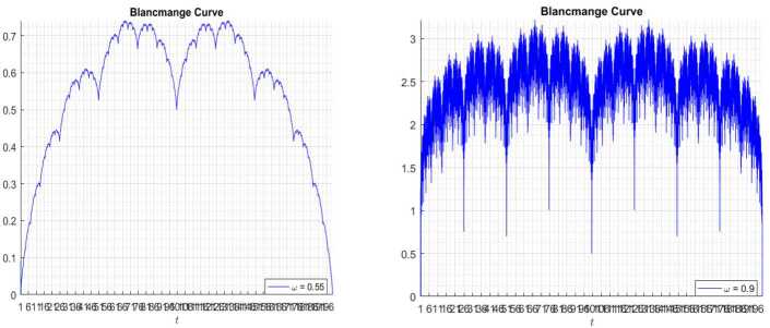
where c is the real number. We now present the extended blancmange function for different periodic parameters and different w.

The simulation are presented in Figs. 19, 20, 21, and 18.

Figure 19.

Blancmange function $c=2$

Figure 20.

Blancmange function $c=3.7$

Figure 21.

Blancmange function $c=1.3$

Mathematical model for COVID-19 outbreak

We consider the following mathematical model of COVID-19 spread:

$$\begin{array}{c}\stackrel{\cdot }{S}=\mathrm{\Lambda }-\{\delta (t)(\alpha I+w(\beta I_D+\gamma I_A+{\delta }_1{I}_R+{\delta }_2{I}_T)+{\gamma }_1+{\mu }_1)\}S,\hfill \\ \stackrel{\cdot }{I}=\delta (t)(\alpha I+w(\beta I_D+\gamma I_A+{\delta }_1{I}_R+{\delta }_2{I}_T))S-(\epsilon +\xi +\lambda +{\mu }_1)I,\hfill \\ \stackrel{\cdot }{I_A}=\xi I-(\theta +\mu +\chi +{\mu }_1)I_A,\hfill \\ \stackrel{\cdot }{I_D}=\epsilon I-(\eta +\phi +{\mu }_1)I_D,\hfill \\ \stackrel{\cdot }{I_R}=\eta I_D+\theta I_A-(v+\xi +{\mu }_1)I_R,\hfill \\ \stackrel{\cdot }{I_T}=\mu I_A+v{I}_R-(\sigma +\tau +{\mu }_1)I_T,\hfill \\ \stackrel{\cdot }{R}=\lambda I+\phi I_D+\chi I_A+\xi I_R+\sigma I_T-(\mathrm{\Phi }+{\mu }_1)R,\hfill \\ \stackrel{\cdot }{D}=\tau I_T,\hfill \\ \stackrel{\cdot }{V}={\gamma }_{1}S+\mathrm{\Phi }R-{\mu }_{1}V.\hfill \end{array}$$ 26

The above model was suggested by Atangana and Seda, the model has a deterministic character. In this section, we convert the model to a stochastic one by introducing the effect of environmental white noise. To achieve this, we reformulate the model by adding the nonlinear perturbation into each equation of the system. The perturbation may depend on square of the classes S, I, $I_A$, $I_D$, $I_R$, $I_T$, R, D, and V respectively. Here, we perturb only the rate of each class. However, for the vaccine class, it will be perturbed by a natural death rate.

$$\begin{array}{c}\text{For the class }S(t):-{\gamma }_1\to -{\gamma }_1+({\mathrm{\Pi }}_{11}S+{\mathrm{\Pi }}_{12}){\stackrel{\cdot }{B}}_1(t),\hfill \\ \text{For the class }I(t):-\lambda \to -\lambda +({\mathrm{\Pi }}_{21}I+{\mathrm{\Pi }}_{22}){\stackrel{\cdot }{B}}_2(t),\hfill \\ \text{For the class }{I}_A(t):-\theta \to -\theta +({\mathrm{\Pi }}_{31}{I}_A+{\mathrm{\Pi }}_{32}){\stackrel{\cdot }{B}}_3(t),\hfill \\ \text{For the class }{I}_D(t):-\eta \to -\eta +({\mathrm{\Pi }}_{41}{I}_D+{\mathrm{\Pi }}_{42}){\stackrel{\cdot }{B}}_4(t),\hfill \\ \text{For the class }{I}_R(t):-v\to -v+({\mathrm{\Pi }}_{51}{I}_R+{\mathrm{\Pi }}_{52}){\stackrel{\cdot }{B}}_5(t),\hfill \\ \text{For the class }{I}_T(t):-\sigma \to -\sigma +({\mathrm{\Pi }}_{61}{I}_T+{\mathrm{\Pi }}_{62}){\stackrel{\cdot }{B}}_6(t),\hfill \\ \text{For the class }R(t):-\mathrm{\Phi }\to -\mathrm{\Phi }+({\mathrm{\Pi }}_{71}R+{\mathrm{\Pi }}_{72}){\stackrel{\cdot }{B}}_7(t),\hfill \\ \text{For the class }D(t):\tau \to \tau \text{ no change},\hfill \\ \text{For the class }V(t):-{\mu }_1\to -{\mu }_1+({\mathrm{\Pi }}_{81}V+{\mathrm{\Pi }}_{82}){\stackrel{\cdot }{B}}_8(t).\hfill \end{array}$$

Therefore, the associated stochastic model is given as follows:

$$\begin{array}{c}\begin{array}{rl}dS=& [\mathrm{\Lambda }-\{\delta (t)(\alpha I+w(\beta I_D+\gamma I_A+{\delta }_1{I}_R+{\delta }_2{I}_T)+{\gamma }_1+{\mu }_1)\}S]dt\\ & +({\mathrm{\Pi }}_{11}S+{\mathrm{\Pi }}_{12})Sd{B}_1(t),\end{array}\hfill \\ \begin{array}{rl}dI=& [\delta (t)(\alpha I+w(\beta I_D+\gamma I_A+{\delta }_1{I}_R+{\delta }_2{I}_T))S-(\epsilon +\xi +\lambda +{\mu }_1)I]dt\\ & +({\mathrm{\Pi }}_{21}I+{\mathrm{\Pi }}_{22})Id{B}_2(t),\end{array}\hfill \\ d{I}_A=[\xi I-(\theta +\mu +\chi +{\mu }_1)I_A]dt+({\mathrm{\Pi }}_{31}{I}_A+{\mathrm{\Pi }}_{32})I_{A}d{B}_3(t),\hfill \\ d{I}_D=[\epsilon I-(\eta +\phi +{\mu }_1)I_D]dt+({\mathrm{\Pi }}_{41}{I}_D+{\mathrm{\Pi }}_{42})I_{D}d{B}_4(t),\hfill \\ d{I}_R=[\eta I_D+\theta I_A-(v+\xi +{\mu }_1)I_R]dt+({\mathrm{\Pi }}_{51}{I}_R+{\mathrm{\Pi }}_{52})I_{D}d{B}_5(t),\hfill \\ d{I}_T=[\mu I_A+v{I}_R-(\sigma +\tau +{\mu }_1)I_T]dt+({\mathrm{\Pi }}_{61}{I}_T+{\mathrm{\Pi }}_{62})I_{T}d{B}_6(t),\hfill \\ dR=[\lambda I+\phi I_D+\chi I_A+\xi I_R+\sigma I_T-(\mathrm{\Phi }+{\mu }_1)R]dt+({\mathrm{\Pi }}_{71}R+{\mathrm{\Pi }}_{72})Rd{B}_7(t),\hfill \\ dV=[{\gamma }_{1}S+\mathrm{\Phi }R-{\mu }_{1}V]dt++({\mathrm{\Pi }}_{71}V+{\mathrm{\Pi }}_{72})Vd{B}_8(t).\hfill \end{array}$$ 27

In this conversion, the function $B_i(t)$ represents the standard Brownian motions valid within the set of probability $(\mathrm{\Omega },A,{\{A_t\}}_{t\ge 0},P)$, where ${\{A_t\}}_{t\ge 0}$ is filtration valid under the condition described in [17]. Here, ${\mathrm{\Pi }}_{i,j\in [1,2,3,4,5,6,7,8]}$ are positive and are the intensities of the environmental random disturbance.

Existence and uniqueness

In this subsection, we present the existence and uniqueness of the system solutions of the stochastic model. To achieve the existence and uniqueness, we convert the system into Volterra type. But first we do the following for simplicity:

$$\begin{array}{c}dS=F_1(t,S,I,I_A,I_D,I_R,I_T,R,V)dt+G_1(t,S)d{B}_1(t),\hfill \\ dI=F_2(t,S,I,I_A,I_D,I_R,I_T,R,V)dt+G_2(t,I)d{B}_2(t),\hfill \\ d{I}_A=F_3(t,I,I_A)dt+G_3(t,I_A)d{B}_3(t),\hfill \\ d{I}_D=F_4(t,I,I_D,)dt+G_4(t,I_D)d{B}_4(t),\hfill \\ d{I}_R=F_5(t,I_A,I_D,I_R)dt+G_5(t,I_R)d{B}_5(t),\hfill \\ d{I}_T=F_6(t,I_A,I_R,I_T)dt+G_6(t,I_T)d{B}_6(t),\hfill \\ dR=F_7(t,I,I_A,I_D,I_R,I_T,R)dt+G_7(t,R)d{B}_7(t),\hfill \\ dV=F_8(t,S,R,V)dt+G_8(t,V)d{B}_8(t).\hfill \end{array}$$ 28

Therefore, converting to Volterra, we get

$$\begin{array}{c}S(t)=S(0)+{\int }_0^t{F}_1(\tau ,S,I,I_A,I_D,I_R,I_T,R,V)d\tau +{\int }_0^t{G}_1(\tau ,S)d{B}_1(\tau ),\hfill \\ I(t)=I(0)+{\int }_0^t{F}_2(\tau ,S,I,I_A,I_D,I_R,I_T,R,V)d\tau +{\int }_0^t{G}_2(\tau ,I)d{B}_2(\tau ),\hfill \\ I_A(t)=I_A(0)+{\int }_0^t{F}_3(\tau ,I,I_A)d\tau +{\int }_0^t{G}_3(\tau ,I_A)d{B}_3(\tau ),\hfill \\ I_D(t)=I_D(0)+{\int }_0^t{F}_4(\tau ,I,I_D)d\tau +{\int }_0^t{G}_4(\tau ,I_D)d{B}_4(\tau ),\hfill \\ I_R(t)=I_R(0)+{\int }_0^t{F}_5(\tau ,I_A,I_D,I_R)d\tau +{\int }_0^t{G}_5(\tau ,I_R)d{B}_5(\tau ),\hfill \\ I_T(t)=I_T(0)+{\int }_0^t{F}_6(\tau ,I_A,I_R,I_T)d\tau +{\int }_0^t{G}_6(\tau ,I_T)d{B}_6(\tau ),\hfill \\ R(t)=R(0)+{\int }_0^t{F}_7(\tau ,I,I_A,I_D,I_R,I_T,R)d\tau +{\int }_0^t{G}_7(\tau ,R)d{B}_7(\tau ),\hfill \\ V(t)=V(0)+{\int }_0^t{F}_8(\tau ,S,R,V)d\tau +{\int }_0^t{G}_8(\tau ,S)d{B}_8(\tau ).\hfill \end{array}$$ 29

We present the existence and uniqueness of the stochastic system of COVID-19 model. This will be achieved via the following theorem.

Theorem

Assume that there exist positive constants $K_i$, ${\bar{K}}_i$ such that

• (i)
  $$\begin{array}{c}|F_i(x,t)-F_i(x_i,t){|}^2<K_i|x-x_i{|}^2,\hfill \\ |G_i(x,t)-G_i(x_i,t){|}^2<{\bar{K}}_i|x-x_i{|}^2\hfill \end{array}$$ 30
• (ii)
  $\mathrm{\forall }(x,t)\in R^8\times [0,T]$

  $$|F_i(x,t){|}^2,|G_i(x,t){|}^2<K(1+|x{|}^2).$$ 31

Then there exists a unique solution $X(t)\in R^8$ for our model and it belongs to $M^2([0,T],R^8)$.

The proof can be found in [17], but we have to verify (i) and (ii) for our system. Without loss of generality, we start our investigation with functions $F_1(t,S,I,I_A,I_D,I_R,I_T,R,V)$ and $G_1(t,S)$. For the function F, the proof will be performed for $(t,S)$. Thus

$$|F_1(t,S)-F_1(t,S_1){|}^2=|\delta (t)(\alpha I+w(\beta I_D+\gamma I_A+{\delta }_1{I}_R+{\delta }_2{I}_T)+{\gamma }_1+{\mu }_1)(S-S_1){|}^2.$$ 32

We define the following norm:

$${\parallel \phi \parallel }_{\mathrm{\infty }}=\underset{t\in [0,T]}{sup}|\phi {|}^2,$$ 33

then

$$\begin{array}{rcl}|F_1(S,t)-F_1(S_1,t){|}^2& \le & \underset{t\in [0,T]}{sup}|\delta (t)(\alpha I+w(\beta I_D+\gamma I_A+{\delta }_1{I}_R+{\delta }_2{I}_T))(S-S_1){|}^2\\ & \le & {\parallel \delta (t)(\alpha I+w(\beta I_D+\gamma I_A+{\delta }_1{I}_R+{\delta }_2{I}_T))\parallel }_{\mathrm{\infty }}^2|S-S_1{|}^2\\ & \le & K_1|S-S_1{|}^2\end{array}$$ 34

and

$$\begin{array}{rcl}|G_1(S,t)-G_1(S_1,t){|}^2& =& |({\mathrm{\Pi }}_{11}S+{\mathrm{\Pi }}_{12})S-({\mathrm{\Pi }}_{11}{S}_1+{\mathrm{\Pi }}_{12})S_1{|}^2\\ & =& |{\mathrm{\Pi }}_{11}(S^2-S_1^2)-{\mathrm{\Pi }}_{12}(S-S_1){|}^2\\ & =& {({\mathrm{\Pi }}_{11}(S+S_1)+{\mathrm{\Pi }}_{12})}^2|S-S_1{|}^2\\ & =& ({\mathrm{\Pi }}_{11}^2{(S+S_1)}^2+2{\mathrm{\Pi }}_{11}{\mathrm{\Pi }}_{12}(S+S_1)+{\mathrm{\Pi }}_{12}^2)|S-S_1{|}^2\\ & =& ({\mathrm{\Pi }}_{11}^2(S^2+2S{S}_1+S_1^2)+2{\mathrm{\Pi }}_{11}{\mathrm{\Pi }}_{12}(S+S_1)+{\mathrm{\Pi }}_{12}^2)|S-S_1{|}^2\\ & \le & \left\{\begin{array}{c}{\mathrm{\Pi }}_{11}^2\left(\begin{array}{c}{sup}_{t\in [0,T]}|S^2(t)|+2{sup}_{t\in [0,T]}|S(t)|{sup}_{t\in [0,T]}|S_1(t)|\\ +{sup}_{t\in [0,T]}|S_1^2(t)|\end{array}\right)\\ +2{\mathrm{\Pi }}_{11}{\mathrm{\Pi }}_{12}\left({sup}_{t\in [0,T]}\right|S(t)|+{sup}_{t\in [0,T]}|S_1(t)\left|\right)+{\mathrm{\Pi }}_{12}^2\end{array}\right\}\\ & & \times |S-S_1{|}^2\\ & \le & \left\{\begin{array}{c}{\mathrm{\Pi }}_{11}^2({\parallel S^2\parallel }_{\mathrm{\infty }}+2{\parallel S\parallel }_{\mathrm{\infty }}{\parallel S_1\parallel }_{\mathrm{\infty }}+{\parallel S_1^2\parallel }_{\mathrm{\infty }})\\ +2{\mathrm{\Pi }}_{11}{\mathrm{\Pi }}_{12}{\parallel S\parallel }_{\mathrm{\infty }}{\parallel S_1\parallel }_{\mathrm{\infty }}+{\mathrm{\Pi }}_{12}^2\end{array}\right\}|S-S_1{|}^2\\ & \le & {\bar{K}}_1|S-S_1{|}^2,\end{array}$$ 35

where

$$\begin{array}{rcl}{\bar{K}}_1& =& {\mathrm{\Pi }}_{11}^2({\parallel S^2\parallel }_{\mathrm{\infty }}+2{\parallel S\parallel }_{\mathrm{\infty }}{\parallel S_1\parallel }_{\mathrm{\infty }}+{\parallel S_1^2\parallel }_{\mathrm{\infty }})+2{\mathrm{\Pi }}_{11}{\mathrm{\Pi }}_{12}{\parallel S\parallel }_{\mathrm{\infty }}{\parallel S_1\parallel }_{\mathrm{\infty }}+{\mathrm{\Pi }}_{12}^2\\ & =& {\mathrm{\Pi }}_{11}^2{({\parallel S\parallel }_{\mathrm{\infty }}+{\parallel S_1\parallel }_{\mathrm{\infty }})}^2+2{\mathrm{\Pi }}_{11}{\mathrm{\Pi }}_{12}{\parallel S\parallel }_{\mathrm{\infty }}{\parallel S_1\parallel }_{\mathrm{\infty }}+{\mathrm{\Pi }}_{12}^2.\end{array}$$ 36

Similarly,

$$\begin{array}{c}{\bar{K}}_2={\mathrm{\Pi }}_{21}^2{({\parallel I\parallel }_{\mathrm{\infty }}+{\parallel I_1\parallel }_{\mathrm{\infty }})}^2+2{\mathrm{\Pi }}_{21}{\mathrm{\Pi }}_{22}{\parallel I\parallel }_{\mathrm{\infty }}{\parallel I_1\parallel }_{\mathrm{\infty }}+{\mathrm{\Pi }}_{22}^2,\hfill \\ {\bar{K}}_3={\mathrm{\Pi }}_{31}^2{({\parallel I_A\parallel }_{\mathrm{\infty }}+{\parallel I_{A1}\parallel }_{\mathrm{\infty }})}^2+2{\mathrm{\Pi }}_{31}{\mathrm{\Pi }}_{32}{\parallel I_A\parallel }_{\mathrm{\infty }}{\parallel I_{A1}\parallel }_{\mathrm{\infty }}+{\mathrm{\Pi }}_{32}^2,\hfill \\ {\bar{K}}_4={\mathrm{\Pi }}_{41}^2{({\parallel I_D\parallel }_{\mathrm{\infty }}+{\parallel I_{D1}\parallel }_{\mathrm{\infty }})}^2+2{\mathrm{\Pi }}_{41}{\mathrm{\Pi }}_{42}{\parallel I_D\parallel }_{\mathrm{\infty }}{\parallel I_{D1}\parallel }_{\mathrm{\infty }}+{\mathrm{\Pi }}_{42}^2,\hfill \\ {\bar{K}}_5={\mathrm{\Pi }}_{51}^2{({\parallel I_R\parallel }_{\mathrm{\infty }}+{\parallel I_{R1}\parallel }_{\mathrm{\infty }})}^2+2{\mathrm{\Pi }}_{51}{\mathrm{\Pi }}_{52}{\parallel I_R\parallel }_{\mathrm{\infty }}{\parallel I_{R1}\parallel }_{\mathrm{\infty }}+{\mathrm{\Pi }}_{52}^2,\hfill \\ {\bar{K}}_6={\mathrm{\Pi }}_{61}^2{({\parallel I_T\parallel }_{\mathrm{\infty }}+{\parallel I_{T1}\parallel }_{\mathrm{\infty }})}^2+2{\mathrm{\Pi }}_{61}{\mathrm{\Pi }}_{62}{\parallel I_T\parallel }_{\mathrm{\infty }}{\parallel I_{T1}\parallel }_{\mathrm{\infty }}+{\mathrm{\Pi }}_{62}^2,\hfill \\ {\bar{K}}_7={\mathrm{\Pi }}_{71}^2{({\parallel R\parallel }_{\mathrm{\infty }}+{\parallel R_1\parallel }_{\mathrm{\infty }})}^2+2{\mathrm{\Pi }}_{71}{\mathrm{\Pi }}_{72}{\parallel R\parallel }_{\mathrm{\infty }}{\parallel R_1\parallel }_{\mathrm{\infty }}+{\mathrm{\Pi }}_{72}^2,\hfill \\ {\bar{K}}_8={\mathrm{\Pi }}_{81}^2{({\parallel V\parallel }_{\mathrm{\infty }}+{\parallel V_1\parallel }_{\mathrm{\infty }})}^2+2{\mathrm{\Pi }}_{81}{\mathrm{\Pi }}_{82}{\parallel V\parallel }_{\mathrm{\infty }}{\parallel V_1\parallel }_{\mathrm{\infty }}+{\mathrm{\Pi }}_{82}^2.\hfill \end{array}$$ 37

Also

$$\begin{array}{rcl}|F_2(I,t)-F_2(I_1,t){|}^2& =& |\delta (t)\alpha (I-I_1)-(\epsilon +\xi +\lambda +{\mu }_1)(I-I_1){|}^2\\ & =& |(\delta (t)\alpha -(\epsilon +\xi +\lambda +{\mu }_1))(I-I_1){|}^2\\ & \le & \underset{t\in [0,T]}{sup}|(\delta (t)\alpha -(\epsilon +\xi +\lambda +{\mu }_1)){|}^2|I-I_1{|}^2\\ & \le & {\parallel \delta (t)\parallel }_{\mathrm{\infty }}|\alpha -(\epsilon +\xi +\lambda +{\mu }_1){|}^2|I-I_1{|}^2\\ & \le & K_2|I-I_1{|}^2,\end{array}$$ 38

where

$$K_2={\parallel \delta (t)\parallel }_{\mathrm{\infty }}|\alpha -(\epsilon +\xi +\lambda +{\mu }_1){|}^2.$$ 39

Also

$$\begin{array}{rcl}|F_3(I_A,t)-F_3(I_{A1},t){|}^2& =& |-(\theta +\mu +\chi +{\mu }_1)(I_A-I_{A1}){|}^2\\ & \le & 2|(\theta +\mu +\chi +{\mu }_1){|}^2|I_A-I_{A1}{|}^2\\ & \le & K_3|I_A-I_{A1}{|}^2,\end{array}$$ 40

where

$$K_3=2|(\theta +\mu +\chi +{\mu }_1){|}^2.$$ 41

Similarly, we evaluate

$$\begin{array}{c}\begin{array}{rl}|F_4(I_D,t)-F_4(I_{D1},t){|}^2=& |\eta +\phi +{\mu }_1{|}^2|I_D-I_{D1}{|}^2\\ \le & K_4|I_D-I_{D1}{|}^2,\end{array}\hfill \\ \begin{array}{rl}|F_5(I_R,t)-F_5(I_{R1},t){|}^2& =|v+\xi +{\mu }_1{|}^2|I_R-I_{R1}{|}^2\\ & \le K_5|I_R-I_{R1}{|}^2,\end{array}\hfill \\ \begin{array}{rl}|F_6(I_T,t)-F_6(I_{T1},t){|}^2& =|\sigma +\tau +{\mu }_1{|}^2|I_T-I_{T1}{|}^2\\ & \le K_6|I_T-I_{T1}|,\end{array}\hfill \\ \begin{array}{rl}|F_7(R,t)-F_7(R_1,t){|}^2& =|\mathrm{\Phi }+{\mu }_1{|}^2|R-R_1{|}^2\\ & \le K_7|R-R_1|,\end{array}\hfill \\ \begin{array}{rl}|F_8(V,t)-F_8(V_1,t){|}^2& =|{\mu }_1{|}^2|V-V_1{|}^2\\ & \le K_8|V-V_1{|}^2.\end{array}\hfill \end{array}$$ 42

For both classes $G_i$ and $F_i$, we have verified condition (i). Now we verify the second condition.

$$\begin{array}{rcl}|F_1(S,t){|}^2& =& |\mathrm{\Lambda }-\delta (t)(\alpha I+w(\beta I_D+\gamma I_A+{\delta }_1{I}_R+{\delta }_2{I}_T)+{\gamma }_1+{\mu }_1)S{|}^2\\ & \le & |\mathrm{\Lambda }S-\delta (t)(\alpha I+w(\beta I_D+\gamma I_A+{\delta }_1{I}_R+{\delta }_2{I}_T)+{\gamma }_1+{\mu }_1)S{|}^2\\ & \le & |S{|}^2|\mathrm{\Lambda }-\delta (t)(\alpha I+w(\beta I_D+\gamma I_A+{\delta }_1{I}_R+{\delta }_2{I}_T)+{\gamma }_1+{\mu }_1){|}^2\\ & <& (|S{|}^2+1)|\mathrm{\Lambda }-\delta (t)(\alpha I+w(\beta I_D+\gamma I_A+{\delta }_1{I}_R+{\delta }_2{I}_T)+{\gamma }_1+{\mu }_1){|}^2\\ & <& (|S{|}^2+1)|\mathrm{\Lambda }-\delta (t)(\alpha I+w(\beta I_D+\gamma I_A+{\delta }_1{I}_R+{\delta }_2{I}_T)+{\gamma }_1+{\mu }_1){|}^2\\ & <& (|S{|}^2+1)\underset{t\in [0,T]}{sup}|\mathrm{\Lambda }-\delta (t)(\alpha I+w(\beta I_D+\gamma I_A+{\delta }_1{I}_R+{\delta }_2{I}_T)+{\gamma }_1+{\mu }_1){|}^2\\ & <& K^1(|S{|}^2+1),\end{array}$$ 43

where

$$K^1=\underset{t\in [0,T]}{sup}|\mathrm{\Lambda }-\delta (t)(\alpha I+w(\beta I_D+\gamma I_A+{\delta }_1{I}_R+{\delta }_2{I}_T)+{\gamma }_1+{\mu }_1){|}^2.$$ 44

Then

$$\begin{array}{rcl}|G_1(S,t)-G_1(S_1,t){|}^2& =& |({\mathrm{\Pi }}_{11}S+{\mathrm{\Pi }}_{12})S{|}^2\\ & \le & |{\mathrm{\Pi }}_{11}{S}^2+{\mathrm{\Pi }}_{12}{S}^2{|}^2\\ & \le & {({\mathrm{\Pi }}_{11}+{\mathrm{\Pi }}_{12})}^2|S^2{|}^2\\ & \le & {({\mathrm{\Pi }}_{11}+{\mathrm{\Pi }}_{12})}^2\underset{t\in [0,T]}{sup}\left|S^2\right||S{|}^2\\ & \le & {({\mathrm{\Pi }}_{11}+{\mathrm{\Pi }}_{12})}^2{\parallel S^2\parallel }_{\mathrm{\infty }}(|S{|}^2+1)\\ & \le & {\bar{K}}^1(|S{|}^2+1),\end{array}$$ 45

where

$${\bar{K}}^1={({\mathrm{\Pi }}_{11}+{\mathrm{\Pi }}_{12})}^2{\parallel S^2\parallel }_{\mathrm{\infty }}.$$ 46

Similarly,

$$\begin{array}{c}{\bar{K}}^2={({\mathrm{\Pi }}_{21}+{\mathrm{\Pi }}_{22})}^2{\parallel I^2\parallel }_{\mathrm{\infty }},\hfill \\ {\bar{K}}^3={({\mathrm{\Pi }}_{31}+{\mathrm{\Pi }}_{32})}^2{\parallel I_A^2\parallel }_{\mathrm{\infty }},\hfill \\ {\bar{K}}^4={({\mathrm{\Pi }}_{41}+{\mathrm{\Pi }}_{42})}^2{\parallel I_D^2\parallel }_{\mathrm{\infty }},\hfill \\ {\bar{K}}^5={({\mathrm{\Pi }}_{51}+{\mathrm{\Pi }}_{52})}^2{\parallel I_R^2\parallel }_{\mathrm{\infty }},\hfill \\ {\bar{K}}^6={({\mathrm{\Pi }}_{61}+{\mathrm{\Pi }}_{62})}^2{\parallel I_T^2\parallel }_{\mathrm{\infty }},\hfill \\ {\bar{K}}^7={({\mathrm{\Pi }}_{71}+{\mathrm{\Pi }}_{72})}^2{\parallel R^2\parallel }_{\mathrm{\infty }},\hfill \\ {\bar{K}}^8={({\mathrm{\Pi }}_{81}+{\mathrm{\Pi }}_{82})}^2{\parallel V^2\parallel }_{\mathrm{\infty }}.\hfill \end{array}$$ 47

Also, we have

$$\begin{array}{c}\begin{array}{rl}|F_2(I,t){|}^2& =|\delta (t)(w(\beta I_D+\gamma I_A+{\delta }_1{I}_R+{\delta }_2{I}_T))S+\delta (t)\alpha IS-(\epsilon +\xi +\lambda +{\mu }_1)I{|}^2\\ & \le |\delta (t)(w(\beta I_D+\gamma I_A+{\delta }_1{I}_R+{\delta }_2{I}_T))S+\delta (t)\alpha S-(\epsilon +\xi +\lambda +{\mu }_1)||I{|}^2\\ & <(|S{|}^2+1)\underset{t\in [0,T]}{sup}|\delta (t)(w(\beta I_D+\gamma I_A+{\delta }_1{I}_R+{\delta }_2{I}_T))S+\delta (t)\alpha S\\ & -(\epsilon +\xi +\lambda +{\mu }_1){|}^2\\ & <K^2(|I{|}^2+1),\end{array}\hfill \\ \begin{array}{rl}|F_3(I_A,t){|}^2& =|\xi I-(\theta +\mu +\chi +{\mu }_1)I_A{|}^2\\ & \le |\xi I-(\theta +\mu +\chi +{\mu }_1){|}^2|I_A{|}^2\\ & \le (|I_A{|}^2+1)\underset{t\in [0,T]}{sup}|\xi I-(\theta +\mu +\chi +{\mu }_1){|}^2\\ & \le K^3(|I_A{|}^2+1),\end{array}\hfill \\ \begin{array}{rl}|F_4(I_A,t){|}^2& =|\epsilon I-(\eta +\phi +{\mu }_1)I_D{|}^2\\ & \le (|I_D{|}^2+1)\underset{t\in [0,T]}{sup}|\epsilon I-(\eta +\phi +{\mu }_1){|}^2\\ & \le K^4(|I_D{|}^2+1),\end{array}\hfill \\ \begin{array}{rl}|F_5(I_R,t){|}^2& \le (|I_R{|}^2+1)\underset{t\in [0,T]}{sup}|\eta I_D+\theta I_A-(v+\xi +{\mu }_1){|}^2\\ & \le K^5(|I_R{|}^2+1),\end{array}\hfill \\ \begin{array}{rl}|F_6(I_T,t){|}^2& \le (|I_T{|}^2+1)\underset{t\in [0,T]}{sup}|\mu I_A+v{I}_R-(\sigma +\tau +{\mu }_1){|}^2\\ & \le K^6(|I_T{|}^2+1),\end{array}\hfill \\ \begin{array}{rl}|F_6(I_T,t){|}^2& \le (|I_T{|}^2+1)\underset{t\in [0,T]}{sup}|\mu I_A+v{I}_R-(\sigma +\tau +{\mu }_1){|}^2\\ & \le K^6(|I_T{|}^2+1),\end{array}\hfill \\ \begin{array}{rl}|F_7(R,t){|}^2& \le (|R{|}^2+1)\underset{t\in [0,T]}{sup}|\lambda I+\phi I_D+\chi I_A+\xi I_R+\sigma I_T-(\mathrm{\Phi }+{\mu }_1){|}^2\\ & \le K^7(|R{|}^2+1).\end{array}\hfill \end{array}$$ 48

Finally, we have

$$\begin{array}{rcl}|F_8(V,t){|}^2& \le & (|V{|}^2+1)\underset{t\in [0,T]}{sup}|{\gamma }_{1}S+\mathrm{\Phi }R-{\mu }_1{|}^2\\ & \le & K^8(|V{|}^2+1).\end{array}$$

Both $G_i$ and $F_i$ verify the second condition. Therefore, according to the above theorem, the system has a unique system solution.

Numerical simulation for the stochastic model

Numerical solutions of the suggested stochastic model are presented in Figs. 22–25. The numerical solution depicts the future stochastic behavior of the susceptible class, five sub-classes of the infected population, the recovered class, the death class, and the vaccination class. These are depicted in figures below.

Figure 23.

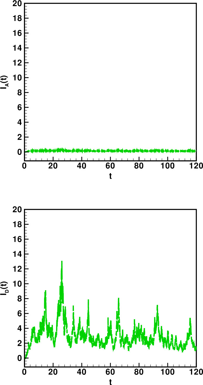
Stochastic behavior of $I_A(t)$ and $I_D(t)$ classes

Figure 24.

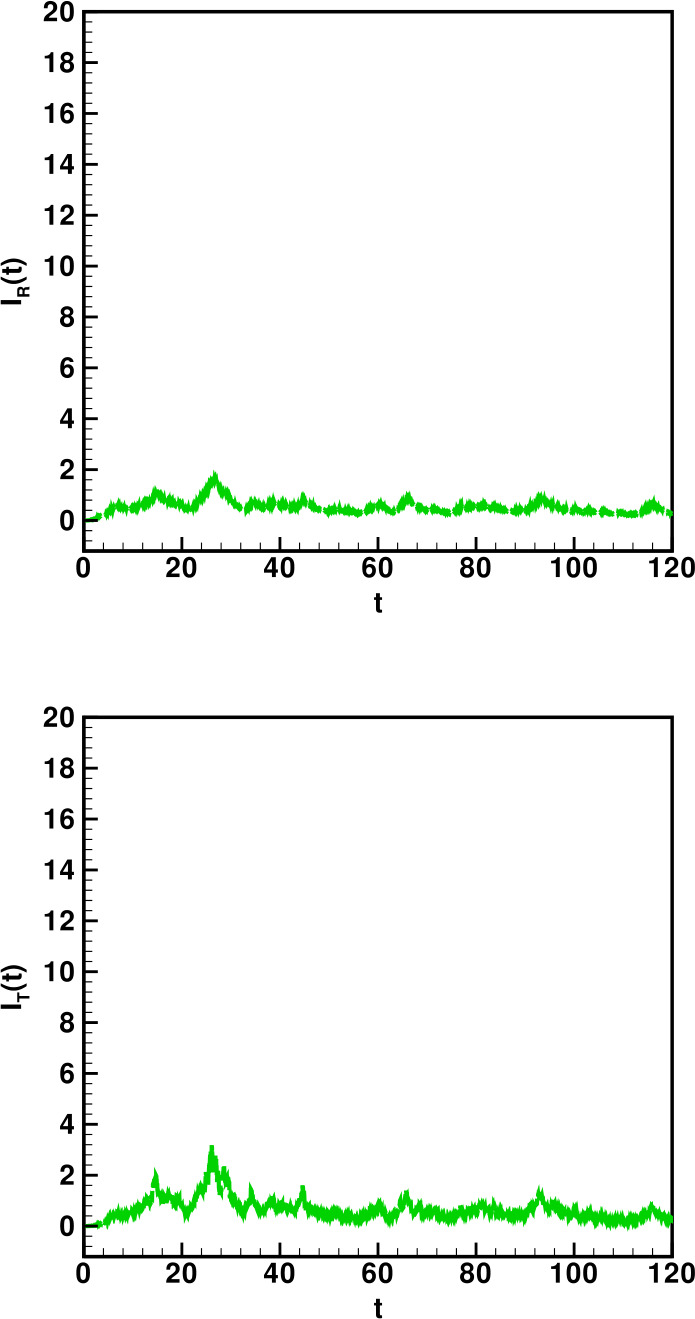
Stochastic behavior of $I_R(t)$ and $I_T(t)$ classes

Figure 22.

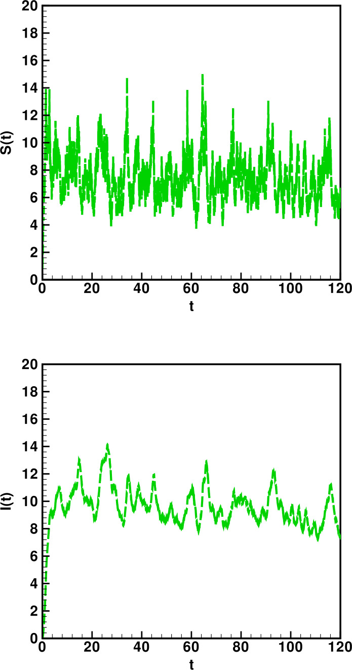
Stochastic behavior of $S(t)$ and $I(t)$ classes

Figure 25.

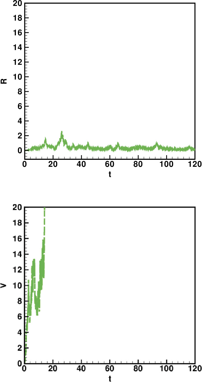
Stochastic behavior of $R(t)$ and $V(t)$ classes

Atangana–Seda modified scheme

The mathematical model considered in this work has the ability to depict two to three waves of COVID-19 spread. The model is subjected to a system of initial conditions. Additionally, the model is nonlinear, thus it is impossible to obtain exact solutions to the system, thus numerical schemes are needed. We present a numerical scheme based on the Newton polynomial [18]. However, one needs the initial condition and two additional components for the scheme to be implemented. In this section, we present a modified version that will not need the two additional components, and then the scheme will be used later to provide numerical solutions for the suggested COVID-19 model with different differential operators. We start with the classical case, the following is considered:

$$\frac{dy(t)}{dt}=f(t,y(t)).$$ 49

Then

$$y^{n+1}=y^n+\{\frac{5}{12}f(t_{n-2},y^{n-2})-\frac{4}{3}f(t_{n-1},y^{n-1})+\frac{5}{12}f(t_n,y^n)\}\mathrm{\Delta }t.$$ 50

To reduce these requirements, we proceed as follows:

$$\frac{y^n-y^{n-1}}{\mathrm{\Delta }t}=f(t_n,y^n)\Rightarrow y^{n-1}=y^n-f(t_n,y^n)\mathrm{\Delta }t.$$ 51

On the other hand,

$$\frac{y^{n-1}-y^{n-2}}{\mathrm{\Delta }t}=f(t_{n-1},y^{n-1})$$ 52

or

$$\begin{array}{rcl}{y}^{n-2}& =& y^{n-1}-f(t_{n-1},y^{n-1})\mathrm{\Delta }t\\ & =& y^n-\mathrm{\Delta }tf(t_n,y^n)-\mathrm{\Delta }tf(t_{n-1},y^n-f(t_n,y^n)\mathrm{\Delta }t).\end{array}$$ 53

Replacing $y^{n-2}$ and $y^{n-1}$ with their values, we obtain

$$\begin{array}{rcl}{y}^{n+1}& =& y^n+\frac{5}{12}\mathrm{\Delta }tf(t_{n-2},y^n-\mathrm{\Delta }tf(t_n,y^n)-\mathrm{\Delta }tf(t_{n-1},y^n-f(t_n,y^n)\mathrm{\Delta }t))\\ & & -\frac{4}{3}f(t_{n-1},y^n-f(t_n,y^n)\mathrm{\Delta }t)+\frac{23}{12}f(t_n,y^n)\mathrm{\Delta }t.\end{array}$$ 54

The above does not need $y^1$ and $y^2$, only the initial condition. With the Caputo–Fabrizio derivative, we consider the following:

$${}_0{}^{CF}D_t^{\alpha }y(t)=f(t,y(t)).$$ 55

From the definition of the Caputo–Fabrizio integral, we can reformulate the above equation as follows:

$$y(t)-y(0)=\frac{1-\alpha }{M(\alpha )}f(t,y(t))+\frac{\alpha }{M(\alpha )}{\int }_0^{t}f(\tau ,y(\tau ))d\tau .$$ 56

We have, at the point $t_{n+1}=(n+1)\mathrm{\Delta }t$,

$$y(t_{n+1})-y(0)=\frac{1-\alpha }{M(\alpha )}f(t_{n+1},y(t_{n+1}))+\frac{\alpha }{M(\alpha )}{\int }_0^{t_{n+1}}f(\tau ,y(\tau ))d\tau ,$$ 57

and at the point $t_n=n\mathrm{\Delta }t$,

$$y(t_n)-y(0)=\frac{1-\alpha }{M(\alpha )}f(t_n,y(t_n))+\frac{\alpha }{M(\alpha )}{\int }_0^{t_n}f(\tau ,y(\tau ))d\tau .$$ 58

Taking the difference of these equations, we can write the following:

$$\begin{array}{rcl}y(t_{n+1})-y(t_n)& =& \frac{1-\alpha }{M(\alpha )}[f(t_{n+1},y(t_{n+1}))-f(t_n,y(t_n))]\\ & & +\frac{\alpha }{M(\alpha )}{\int }_{t_n}^{t_{n+1}}f(\tau ,y(\tau ))d\tau \\ & =& \frac{1-\alpha }{M(\alpha )}\left[\begin{array}{c}f(t_{n+1},y(t_n)-\mathrm{\Delta }tf(t_n,y(t_n)))\\ -f(t_n,y(t_n))\end{array}\right]\\ & & +\frac{\alpha }{M(\alpha )}\left\{\begin{array}{c}\frac{5}{12}f(t_{n-2},y^n-\mathrm{\Delta }tf(t_n,y^n)-\mathrm{\Delta }tf(t_{n-1},y^n-f(t_n,y^n)\mathrm{\Delta }t))\mathrm{\Delta }t\\ -\frac{4}{3}f(t_{n-1},y^n-f(t_n,y^n)\mathrm{\Delta }t)\mathrm{\Delta }t\\ +\frac{23}{12}f(t_n,y^n)\mathrm{\Delta }t\end{array}\right\}.\end{array}$$ 59

With the Caputo derivative, we write

$$\{\begin{array}{c}{}_0{}^{C}D_t^{\alpha }y(t)=f(t,y(t)),\hfill \\ y(0)=y_0.\hfill \end{array}$$ 60

We convert the above into

$$y(t)-y(0)=\frac{1}{\mathrm{\Gamma }(\alpha )}{\int }_0^{t}f(\tau ,y(\tau )){(t-\tau )}^{\alpha -1}d\tau .$$ 61

At the point $t_{n+1}=(n+1)\mathrm{\Delta }t$, we have the following:

$$y(t_{n+1})-y(0)=\frac{1}{\mathrm{\Gamma }(\alpha )}{\int }_0^{t_{n+1}}f(\tau ,y(\tau )){(t_{n+1}-\tau )}^{\alpha -1}d\tau ,$$

and we write

$$y(t_{n+1})=y(0)+\frac{1}{\mathrm{\Gamma }(\alpha )}\sum _{j=2}^n{\int }_{t_j}^{t_{j+1}}f(\tau ,y(\tau )){(t_{n+1}-\tau )}^{\alpha -1}d\tau .$$

After putting the Newton polynomial into the above equation, the above equation can be written as follows:

$$\begin{array}{rl}{y}^{n+1}=& y^0+\frac{{(\mathrm{\Delta }t)}^{\alpha }}{\mathrm{\Gamma }(\alpha +1)}\sum _{j=2}^{n}f(t_{j-2},y^{j-2})[{(n-j+1)}^{\alpha }-{(n-j)}^{\alpha }]\\ & +\frac{{(\mathrm{\Delta }t)}^{\alpha }}{\mathrm{\Gamma }(\alpha +2)}\sum _{j=2}^n[f(t_{j-1},y^{j-1})-f(t_{j-2},y^{j-2})]\\ & \times \left[\begin{array}{c}{(n-j+1)}^{\alpha }(n-j+3+2\alpha )\\ -{(n-j)}^{\alpha }(n-j+3+3\alpha )\end{array}\right]\\ & +\frac{\alpha {(\mathrm{\Delta }t)}^{\alpha }}{2\mathrm{\Gamma }(\alpha +3)}\sum _{j=2}^n\left[\begin{array}{c}f(t_j,y^j)-2f(t_{j-1},y^{j-1})\\ +f(t_{j-2},y^{j-2})\end{array}\right]\\ & \times \left[\begin{array}{c}{(n-j+1)}^{\alpha }\left[\begin{array}{c}2{(n-j)}^2+(3\alpha +10)(n-j)\\ +2{\alpha }^2+9\alpha +12\end{array}\right]\\ -{(n-j)}^{\alpha }\left[\begin{array}{c}2{(n-j)}^2+(5\alpha +10)(n-j)\\ +6{\alpha }^2+18\alpha +12\end{array}\right]\end{array}\right],\end{array}$$ 62

where

$$\begin{array}{c}f(t_{j-1},y^{j-1})=f(t_{j-1},y^j-f(t_j,y^j)\mathrm{\Delta }t),\hfill \\ f(t_{j-2},y^{j-2})=f(t_{j-2},y^j-\mathrm{\Delta }tf(t_j,y^j)-\mathrm{\Delta }tf(t_{j-1},y^j-f(t_j,y^j)\mathrm{\Delta }t)).\hfill \end{array}$$ 63

With Atangana–Baleanu, we have

$$\{\begin{array}{c}{}_0{}^{ABC}D_t^{\alpha }y(t)=f(t,y(t)),\hfill \\ y(0)=y_0.\hfill \end{array}$$ 64

We transform the above equation into

$$y(t)-y(0)=\frac{1-\alpha }{AB(\alpha )}f(t,y(t))+\frac{\alpha }{AB(\alpha )\mathrm{\Gamma }(\alpha )}{\int }_0^{t}f(\tau ,y(\tau )){(t-\tau )}^{\alpha -1}d\tau .$$ 65

At the point $t_{n+1}=(n+1)\mathrm{\Delta }t$, we have the following:

$$\begin{array}{rcl}y(t_{n+1})-y(0)& =& \frac{1-\alpha }{AB(\alpha )}f(t,y(t))\\ & & +\frac{\alpha }{AB(\alpha )\mathrm{\Gamma }(\alpha )}{\int }_0^{t_{n+1}}f(\tau ,y(\tau )){(t_{n+1}-\tau )}^{\alpha -1}d\tau ,\end{array}$$ 66

and we write

$$\begin{array}{rcl}y(t_{n+1})& =& y(0)+\frac{1-\alpha }{AB(\alpha )}f(t_{n+1},y^{n+1})\\ & & +\frac{\alpha }{AB(\alpha )\mathrm{\Gamma }(\alpha )}\sum _{j=2}^n{\int }_{t_j}^{t_{j+1}}f(\tau ,y(\tau )){(t_{n+1}-\tau )}^{\alpha -1}d\tau .\end{array}$$ 67

After putting the Newton polynomial into the above equation, the above equation can be written as follows:

$$\begin{array}{rcl}{y}^{n+1}& =& y^0+\frac{1-\alpha }{AB(\alpha )}f(t_{n+1},y(t_n)-\mathrm{\Delta }tf(t_n,y(t_n)))\\ & & +\frac{\alpha {(\mathrm{\Delta }t)}^{\alpha }}{AB(\alpha )\mathrm{\Gamma }(\alpha +1)}\sum _{j=2}^{n}f\left(\begin{array}{c}{t}_{j-2},y^j-\mathrm{\Delta }tf(t_j,y^j)\\ -\mathrm{\Delta }tf(t_{j-1},y^j-f(t_j,y^j)\mathrm{\Delta }t)\end{array}\right)\\ & & \times [{(n-j+1)}^{\alpha }-{(n-j)}^{\alpha }]\\ & & +\frac{\alpha {(\mathrm{\Delta }t)}^{\alpha }}{AB(\alpha )\mathrm{\Gamma }(\alpha +2)}\sum _{j=2}^n\left[\begin{array}{c}f(t_{j-1},y^j-f(t_j,y^j)\mathrm{\Delta }t)\\ -f(t_{j-2},y^j-\mathrm{\Delta }tf(t_j,y^j)-\mathrm{\Delta }tf(t_{j-1},y^j-f(t_j,y^j)\mathrm{\Delta }t))\end{array}\right]\\ & & \times \left[\begin{array}{c}{(n-j+1)}^{\alpha }(n-j+3+2\alpha )\\ -{(n-j)}^{\alpha }(n-j+3+3\alpha )\end{array}\right]\\ & & +\frac{\alpha {(\mathrm{\Delta }t)}^{\alpha }}{2AB(\alpha )\mathrm{\Gamma }(\alpha +3)}\sum _{j=2}^n\left[\begin{array}{c}f(t_j,y^j)-2f(t_{j-1},y^{j-1})\\ +f\left(\begin{array}{c}{t}_{j-2},y^j-\mathrm{\Delta }tf(t_j,y^j)\\ -\mathrm{\Delta }tf(t_{j-1},y^j-f(t_j,y^j)\mathrm{\Delta }t)\end{array}\right)\end{array}\right]\\ & & \times \left[\begin{array}{c}{(n-j+1)}^{\alpha }\left[\begin{array}{c}2{(n-j)}^2+(3\alpha +10)(n-j)\\ +2{\alpha }^2+9\alpha +12\end{array}\right]\\ -{(n-j)}^{\alpha }\left[\begin{array}{c}2{(n-j)}^2+(5\alpha +10)(n-j)\\ +6{\alpha }^2+18\alpha +12\end{array}\right]\end{array}\right].\end{array}$$ 68

With the Caputo–Fabrizio fractal-fractional derivative, we consider

$$\begin{array}{rl}& {}_0{}^{FFE}D_t^{\alpha ,\beta }y(t)=f(t,y(t)),\\ & y(0)=y_0.\end{array}$$ 69

Applying the associated integral operator with exponential kernel, we can reformulate equation (69) as follows:

$$y(t)=\frac{1-\alpha }{M(\alpha )}{t}^{1-\beta }f(t,y(t))+\frac{\alpha }{M(\alpha )}{\int }_0^{t}f(\tau ,y(\tau )){\tau }^{1-\beta }d\tau .$$ 70

At the point $t_{n+1}=(n+1)\mathrm{\Delta }t$,

$$y(t_{n+1})=\frac{1-\alpha }{M(\alpha )}{t}_{n+1}^{1-\beta }f(t_{n+1},y(t_{n+1}))+\frac{\alpha }{M(\alpha )}{\int }_0^{t_{n+1}}f(\tau ,y(\tau )){\tau }^{1-\beta }d\tau ,$$ 71

and at the point $t_n=n\mathrm{\Delta }t$, we have

$$y(t_n)=\frac{1-\alpha }{M(\alpha )}{t}_n^{1-\beta }f(t_n,y(t_n))+\frac{\alpha }{M(\alpha )}{\int }_0^{t_n}f(\tau ,y(\tau )){\tau }^{1-\beta }d\tau .$$ 72

If we take the difference of these equations, we obtain the following equation:

$$\begin{array}{rcl}y(t_{n+1})-y(t_n)& =& \frac{1-\alpha }{M(\alpha )}\left[\begin{array}{c}{t}_{n+1}^{1-\beta }f(t_{n+1},y(t_{n+1}))\\ -t_n^{1-\beta }f(t_n,y(t_n))\end{array}\right]\\ & & +\frac{\alpha }{M(\alpha )}{\int }_{t_n}^{t_{n+1}}f(\tau ,y(\tau )){\tau }^{1-\beta }d\tau .\end{array}$$ 73

For brevity, we consider

$$\begin{array}{rcl}y(t_{n+1})-y(t_n)& =& \frac{1-\alpha }{M(\alpha )}[F(t_{n+1},y(t_{n+1}))-F(t_n,y(t_n))]\\ & & +\frac{\alpha }{M(\alpha )}{\int }_{t_n}^{t_{n+1}}F(\tau ,y(\tau ))d\tau ,\end{array}$$ 74

where

$$F(t,y(t))=f(t,y(t))t^{1-\beta }.$$ 75

We can rearrange the above scheme as follows:

$$\begin{array}{rcl}{y}^{n+1}-y^n& =& \frac{1-\alpha }{M(\alpha )}\left[\begin{array}{c}F(t_{n+1},y(t_n)-\mathrm{\Delta }tf(t_n,y(t_n)))\\ -F(t_n,y(t_n))\end{array}\right]\\ & & +\frac{\alpha }{M(\alpha )}\left\{\begin{array}{c}\frac{5}{12}F(t_{n-2},y^n-\mathrm{\Delta }tf(t_n,y^n)-\mathrm{\Delta }tF(t_{n-1},y^n-f(t_n,y^n)\mathrm{\Delta }t))\mathrm{\Delta }t\\ -\frac{4}{3}F(t_{n-1},y^n-f(t_n,y^n)\mathrm{\Delta }t)\mathrm{\Delta }t\\ +\frac{23}{12}F(t_n,y^n)\mathrm{\Delta }t\end{array}\right\}.\end{array}$$ 76

If we replace $F(t,y(t))$ with its value, we can solve our equation numerically with the following scheme:

$$\begin{array}{rcl}{y}^{n+1}-y^n& =& \frac{1-\alpha }{M(\alpha )}\left[\begin{array}{c}{t}_{n+1}^{1-\beta }f(t_{n+1},y(t_n)-\mathrm{\Delta }tf(t_n,y(t_n)))\\ -t_n^{1-\beta }f(t_n,y(t_n))\end{array}\right]\\ & & +\frac{\alpha }{M(\alpha )}\left\{\begin{array}{c}{t}_{n-2}^{1-\beta }\frac{5}{12}F(t_{n-2},y^n-\mathrm{\Delta }tf(t_n,y^n)-\mathrm{\Delta }tf(t_{n-1},y^n-f(t_n,y^n)\mathrm{\Delta }t))\mathrm{\Delta }t\\ -\frac{4}{3}{t}_{n-1}^{1-\beta }f(t_{n-1},y^n-f(t_n,y^n)\mathrm{\Delta }t)\mathrm{\Delta }t\\ +\frac{23}{12}{t}_n^{1-\beta }f(t_n,y^n)\mathrm{\Delta }t\end{array}\right\}.\end{array}$$ 77

With the Atangana–Baleanu fractal-fractional derivative, we write

$$\begin{array}{c}{}_0{}^{FFM}D_t^{\alpha ,\beta }y(t)=f(t,y(t)),\hfill \\ y(0)=y_0.\hfill \end{array}$$ 78

Applying the new fractional integral with Mittag-Leffler kernel, we transform the above equation into

$$\begin{array}{rcl}y(t)& =& y(0)+\frac{1-\alpha }{AB(\alpha )}{t}^{1-\beta }f(t,y(t))\\ & & +\frac{\alpha }{AB(\alpha )\mathrm{\Gamma }(\alpha )}{\int }_0^{t}f(\tau ,y(\tau )){(t-\tau )}^{\alpha -1}{\tau }^{1-\beta }d\tau .\end{array}$$ 79

At the point $t_{n+1}=(n+1)\mathrm{\Delta }t$, we obtain the following:

$$\begin{array}{rcl}y(t_{n+1})& =& y(0)+\frac{1-\alpha }{AB(\alpha )}{t}_{n+1}^{1-\beta }f(t_{n+1},y(t_{n+1}))\\ & & +\frac{\alpha }{AB(\alpha )\mathrm{\Gamma }(\alpha )}{\int }_0^{t_{n+1}}f(\tau ,y(\tau )){(t_{n+1}-\tau )}^{\alpha -1}{\tau }^{1-\beta }d\tau .\end{array}$$ 80

For simplicity, we shall take

$$F(t,y(t))=f(t,y(t))t^{1-\beta }.$$ 81

We also have

$$\begin{array}{rcl}y(t_{n+1})& =& y(0)+\frac{1-\alpha }{AB(\alpha )}F(t_{n+1},y(t_{n+1}))\\ & & +\frac{\alpha }{AB(\alpha )\mathrm{\Gamma }(\alpha )}\sum _{j=2}^n{\int }_{t_j}^{t_{j+1}}F(\tau ,y(\tau )){(t_{n+1}-\tau )}^{\alpha -1}d\tau .\end{array}$$ 82

Replacing them into the above equation and substituting $F(t,y(t))=f(t,y(t))t^{1-\beta }$, we can get the following numerical scheme:

$$\begin{array}{rcl}{y}^{n+1}& =& \frac{1-\alpha }{AB(\alpha )}{t}_{n+1}^{1-\beta }f(t_{n+1},y(t_{n+1}))\\ & & +\frac{\alpha {(\mathrm{\Delta }t)}^{\alpha }}{AB(\alpha )\mathrm{\Gamma }(\alpha +1)}\sum _{j=2}^n{t}_{j-2}^{1-\beta }f\left(\begin{array}{c}{t}_{j-2},y^j-\mathrm{\Delta }tf(t_j,y^j)\\ -\mathrm{\Delta }tf(t_{j-1},y^j-f(t_j,y^j)\mathrm{\Delta }t)\end{array}\right)\\ & & \times [{(n-j+1)}^{\alpha }-{(n-j)}^{\alpha }]\\ & & +\frac{\alpha {(\mathrm{\Delta }t)}^{\alpha }}{AB(\alpha )\mathrm{\Gamma }(\alpha +2)}\sum _{j=2}^n\left[\begin{array}{c}{t}_{j-1}^{1-\beta }f(t_{j-1},y^j-f(t_j,y^j)\mathrm{\Delta }t)\\ -t_{j-2}^{1-\beta }f\left(\begin{array}{c}{t}_{j-2},y^j-\mathrm{\Delta }tf(t_j,y^j)\\ -\mathrm{\Delta }tf(t_{j-1},y^j-f(t_j,y^j)\mathrm{\Delta }t)\end{array}\right)\end{array}\right]\\ & & \times \left[\begin{array}{c}{(n-j+1)}^{\alpha }(n-j+3+2\alpha )\\ -{(n-j)}^{\alpha }(n-j+3+3\alpha )\end{array}\right]\\ & & +\frac{\alpha {(\mathrm{\Delta }t)}^{\alpha }}{2AB(\alpha )\mathrm{\Gamma }(\alpha +3)}\sum _{j=2}^n\left[\begin{array}{c}{t}_j^{1-\beta }g(t_j,y^j)\\ -2t_{j-1}^{1-\beta }f(t_{j-1},y^j-f(t_j,y^j)\mathrm{\Delta }t)\\ +t_{j-2}^{1-\beta }f\left(\begin{array}{c}{t}_{j-2},y^j-\mathrm{\Delta }tf(t_j,y^j)\\ -\mathrm{\Delta }tf(t_{j-1},y^j-f(t_j,y^j)\mathrm{\Delta }t)\end{array}\right)\end{array}\right]\\ & & \times \left[\begin{array}{c}{(n-j+1)}^{\alpha }\left[\begin{array}{c}2{(n-j)}^2+(3\alpha +10)(n-j)\\ +2{\alpha }^2+9\alpha +12\end{array}\right]\\ -{(n-j)}^{\alpha }\left[\begin{array}{c}2{(n-j)}^2+(5\alpha +10)(n-j)\\ +6{\alpha }^2+18\alpha +12\end{array}\right]\end{array}\right].\end{array}$$ 83

With the Caputo fractal-fractional derivative, we consider the following:

$$\begin{array}{c}{}_0{}^{FFP}D_t^{\alpha ,\beta }y(t)=f(t,y(t)),\hfill \\ y(0)=y_0.\hfill \end{array}$$ 84

Applying the new fractional integral with power-law kernel, we transform the above equation into

$$y(t)=y(0)+\frac{1}{\mathrm{\Gamma }(\alpha )}{\int }_0^{t}f(\tau ,y(\tau )){(t-\tau )}^{\alpha -1}{\tau }^{1-\beta }d\tau .$$ 85

At the point $t_{n+1}=(n+1)\mathrm{\Delta }t$, we obtain the following:

$$y(t_{n+1})=y(0)+\frac{1}{\mathrm{\Gamma }(\alpha )}{\int }_0^{t_{n+1}}f(\tau ,y(\tau )){(t_{n+1}-\tau )}^{\alpha -1}{\tau }^{1-\beta }d\tau .$$ 86

For simplicity, we shall take

$$F(t,y(t))=f(t,y(t))t^{1-\beta }.$$ 87

We also have

$$y(t_{n+1})=y(0)+\frac{1}{\mathrm{\Gamma }(\alpha )}\sum _{j=2}^n{\int }_{t_j}^{t_{j+1}}F(\tau ,y(\tau )){(t_{n+1}-\tau )}^{\alpha -1}d\tau .$$ 88

Replacing them into the above equation and substituting $F(t,y(t))=f(t,y(t))t^{1-\beta }$, we can get the following numerical scheme:

$$\begin{array}{rcl}{y}^{n+1}& =& \frac{{(\mathrm{\Delta }t)}^{\alpha }}{\mathrm{\Gamma }(\alpha +1)}\sum _{j=2}^n{t}_{j-2}^{1-\beta }f\left(\begin{array}{c}{t}_{j-2},y^j-\mathrm{\Delta }tf(t_j,y^j)\\ -\mathrm{\Delta }tf(t_{j-1},y^j-f(t_j,y^j)\mathrm{\Delta }t)\end{array}\right)\\ & & \times [{(n-j+1)}^{\alpha }-{(n-j)}^{\alpha }]\\ & & +\frac{{(\mathrm{\Delta }t)}^{\alpha }}{\mathrm{\Gamma }(\alpha +2)}\sum _{j=2}^n\left[\begin{array}{c}{t}_{j-1}^{1-\beta }f(t_{j-1},y^j-f(t_j,y^j)\mathrm{\Delta }t)\\ -t_{j-2}^{1-\beta }f\left(\begin{array}{c}{t}_{j-2},y^j-\mathrm{\Delta }tf(t_j,y^j)\\ -\mathrm{\Delta }tf(t_{j-1},y^j-f(t_j,y^j)\mathrm{\Delta }t)\end{array}\right)\end{array}\right]\\ & & \times \left[\begin{array}{c}{(n-j+1)}^{\alpha }(n-j+3+2\alpha )\\ -{(n-j)}^{\alpha }(n-j+3+3\alpha )\end{array}\right]\\ & & +\frac{{(\mathrm{\Delta }t)}^{\alpha }}{2\mathrm{\Gamma }(\alpha +3)}\sum _{j=2}^n\left[\begin{array}{c}{t}_j^{1-\beta }g(t_j,y^j)\\ -2t_{j-1}^{1-\beta }f(t_{j-1},y^j-f(t_j,y^j)\mathrm{\Delta }t)\\ +t_{j-2}^{1-\beta }f\left(\begin{array}{c}{t}_{j-2},y^j-\mathrm{\Delta }tf(t_j,y^j)\\ -\mathrm{\Delta }tf(t_{j-1},y^j-f(t_j,y^j)\mathrm{\Delta }t)\end{array}\right)\end{array}\right]\\ & & \times \left[\begin{array}{c}{(n-j+1)}^{\alpha }\left[\begin{array}{c}2{(n-j)}^2+(3\alpha +10)(n-j)\\ +2{\alpha }^2+9\alpha +12\end{array}\right]\\ -{(n-j)}^{\alpha }\left[\begin{array}{c}2{(n-j)}^2+(5\alpha +10)(n-j)\\ +6{\alpha }^2+18\alpha +12\end{array}\right]\end{array}\right].\end{array}$$ 89

Finally, we present the numerical scheme with fractal-fractional derivative with variable order. We start with the Caputo–Fabrizio case:

$$\begin{array}{c}{}_0{}^{FFE}D_t^{\alpha ,\beta (t)}y(t)=f(t,y(t)),\hfill \\ y(0)=y_0.\hfill \end{array}$$ 90

The above equation can be reformulated as follows:

$$\begin{array}{rcl}y(t)& =& \frac{1-\alpha }{M(\alpha )}{t}^{2-\beta (t)}[-\beta \prime (t)ln(t)+\frac{2-\beta (t)}{t}]f(t,y(t))\\ & & +\frac{\alpha }{M(\alpha )}{\int }_0^{t}f(\tau ,y(\tau ))[\beta \prime (\tau )ln(\tau )+\frac{2-\beta (\tau )}{\tau }]{\tau }^{2-\beta (\tau )}d\tau .\end{array}$$ 91

We write the above equation as follows:

$$\begin{array}{rcl}y(t_{n+1})-y(t_n)& =& \frac{1-\alpha }{M(\alpha )}\left[\begin{array}{c}{t}_{n+1}^{2-\beta (t_{n+1})}(-\frac{\beta (t_{n+2})-\beta (t_{n+1})}{\mathrm{\Delta }t}ln{t}_{n+1}+\frac{2-\beta (t_{n+1})}{t_{n+1}})f(t_{n+1},y(t_{n+1}))\\ -t_n^{2-\beta (t_n)}(-\frac{\beta (t_{n+1})-\beta (t_n)}{\mathrm{\Delta }t}ln{t}_n+\frac{2-\beta (t_n)}{t_n})f(t_n,y(t_n))\end{array}\right]\\ & & +\frac{\alpha }{M(\alpha )}{\int }_{t_n}^{t_{n+1}}f(\tau ,y(\tau ))[\beta \prime (\tau )ln(\tau )+\frac{2-\beta (\tau )}{\tau }]{\tau }^{2-\beta (\tau )}d\tau .\end{array}$$ 92

For simplicity, we take

$$F(t,y(t))=f(t,y(t))[-\beta \prime (t)ln(t)+\frac{2-\beta (t)}{t}]t^{2-\beta (t)},$$ 93

and we have

$$\begin{array}{rcl}y(t_{n+1})-y(t_n)& =& \frac{1-\alpha }{M(\alpha )}[F(t_{n+1},y(t_{n+1}))-F(t_n,y(t_n))]\\ & & +\frac{\alpha }{M(\alpha )}{\int }_{t_n}^{t_{n+1}}F(\tau ,y(\tau ))d\tau .\end{array}$$ 94

If we do the same routine and replace $F(t,y(t))$ with its value, we have the following numerical approximation:

$$\begin{array}{rcl}{y}^{n+1}& =& y^n+\frac{1-\alpha }{M(\alpha )}\left[\begin{array}{c}{t}_{n+1}^{2-\beta (t_{n+1})}(-\frac{\beta (t_{n+2})-\beta (t_{n+1})}{\mathrm{\Delta }t}ln{t}_{n+1}+\frac{2-\beta (t_{n+1})}{t_{n+1}})\\ \times f(t_{n+1},y(t_n)-\mathrm{\Delta }tf(t_n,y(t_n)))\\ -t_n^{2-\beta (t_n)}(-\frac{\beta (t_{n+1})-\beta (t_n)}{\mathrm{\Delta }t}ln{t}_n+\frac{2-\beta (t_n)}{t_n})\\ \times f(t_n,y(t_n))\end{array}\right]\\ & & +\frac{\alpha }{M(\alpha )}\left\{\begin{array}{c}\frac{23}{12}{t}_n^{2-\beta (t_n)}(-\frac{\beta (t_{n+1})-\beta (t_n)}{\mathrm{\Delta }t}ln{t}_n+\frac{2-\beta (t_n)}{t_n})\\ \times \frac{23}{12}f(t_n,y^n)\mathrm{\Delta }t\\ -\frac{4}{3}{t}_{n-1}^{2-\beta (t_{n-1})}(-\frac{\beta (t_n)-\beta (t_{n-1})}{\mathrm{\Delta }t}ln{t}_{n-1}+\frac{2-\beta (t_{n-1})}{t_{n-1}})\\ \times f(t_{n-1},y^n-f(t_n,y^n)\mathrm{\Delta }t)\mathrm{\Delta }t\\ +\frac{5}{12}{t}_{n-2}^{2-\beta (t_{n-2})}(-\frac{\beta (t_{n-1})-\beta (t_{n-2})}{\mathrm{\Delta }t}ln{t}_{n-2}+\frac{2-\beta (t_{n-2})}{t_{n-2}})\\ \times \frac{5}{12}f\left(\begin{array}{c}{t}_{n-2},y^n-\mathrm{\Delta }tf(t_n,y^n)\\ -\mathrm{\Delta }tf(t_{n-1},y^n-f(t_n,y^n)\mathrm{\Delta }t)\end{array}\right)\mathrm{\Delta }t\end{array}\right\}.\end{array}$$ 95

We deal with our problem involving the new constant fractional order and variable fractal dimension

$$\begin{array}{c}{}_0{}^{FFM}D_t^{\alpha ,\beta (t)}y(t)=f(t,y(t)),\hfill \\ y(0)=y_0,\hfill \end{array}$$ 96

where the kernel is the Mittag-Leffler kernel. If we integrate the above equation with the new integral operator including the Mittag-Leffler kernel, the above equation can be converted to

$$\begin{array}{rcl}y(t)& =& \frac{1-\alpha }{AB(\alpha )}{t}^{2-\beta (t)}[-\beta \prime (t)ln(t)+\frac{2-\beta (t)}{t}]f(t,y(t))\\ & & +\frac{\alpha }{AB(\alpha )\mathrm{\Gamma }(\alpha )}{\int }_0^{t}f(\tau ,y(\tau )){(t-\tau )}^{\alpha -1}\\ & & \times [-\beta \prime (\tau )ln(\tau )+\frac{2-\beta (\tau )}{\tau }]{\tau }^{2-\beta (\tau )}d\tau .\end{array}$$ 97

At the point $t_{n+1}=(n+1)\mathrm{\Delta }t$, we have the following:

$$\begin{array}{rcl}y(t_{n+1})& =& \frac{1-\alpha }{AB(\alpha )}{t}_{n+1}^{2-\beta (t_{n+1})}(-\frac{\beta (t_{n+2})-\beta (t_{n+1})}{\mathrm{\Delta }t}ln{t}_{n+1}+\frac{2-\beta (t_{n+1})}{t_{n+1}})\\ & & \times f(t_{n+1},y(t_{n+1}))\\ & & +\frac{\alpha }{AB(\alpha )\mathrm{\Gamma }(\alpha )}{\int }_0^{t_{n+1}}f(\tau ,y(\tau )){(t_{n+1}-s)}^{\alpha -1}\\ & & \times [-\beta \prime (\tau )ln(\tau )+\frac{2-\beta (\tau )}{\tau }]{\tau }^{2-\beta (\tau )}d\tau .\end{array}$$ 98

For brevity, we consider

$$F(\tau ,y(\tau ))=f(\tau ,y(\tau ))[-\beta \prime (\tau )ln(\tau )+\frac{2-\beta (\tau )}{\tau }]{\tau }^{2-\beta (\tau )},$$ 99

and we can write the following:

$$\begin{array}{rcl}y(t_{n+1})& =& \frac{1-\alpha }{AB(\alpha )}{t}_{n+1}^{2-\beta (t_{n+1})}(-\frac{\beta (t_{n+2})-\beta (t_{n+1})}{\mathrm{\Delta }t}ln{t}_{n+1}+\frac{2-\beta (t_{n+1})}{t_{n+1}})\\ & & \times f(t_{n+1},y(t_{n+1}))\\ & & +\frac{\alpha }{AB(\alpha )\mathrm{\Gamma }(\alpha )}\sum _{j=2}^n{\int }_{t_j}^{t_{j+1}}F(\tau ,y(\tau )){(t_{n+1}-\tau )}^{\alpha -1}d\tau .\end{array}$$ 100

One can replace the Newton polynomial in the above equation as follows. Thus, we have the following scheme:

$$\begin{array}{rcl}{y}^{n+1}& =& \frac{1-\alpha }{AB(\alpha )}{t}_{n+1}^{2-\beta (t_{n+1})}(-\frac{\beta (t_{n+2})-\beta (t_{n+1})}{\mathrm{\Delta }t}ln{t}_{n+1}+\frac{2-\beta (t_{n+1})}{t_{n+1}})\\ & & \times f(t_{n+1},y(t_{n+1}))\\ & & +\frac{\alpha {(\mathrm{\Delta }t)}^{\alpha }}{AB(\alpha )\mathrm{\Gamma }(\alpha +1)}\sum _{j=2}^{n}F(t_{j-2},y^{j-2})[{(n-j+1)}^{\alpha }-{(n-j)}^{\alpha }]\\ & & +\frac{\alpha {(\mathrm{\Delta }t)}^{\alpha }}{AB(\alpha )\mathrm{\Gamma }(\alpha +2)}\sum _{j=2}^n[F(t_{j-1},y^{j-1})-F(t_{j-2},y^{j-2})]\\ & & \times \left[\begin{array}{c}{(n-j+1)}^{\alpha }(n-j+3+2\alpha )\\ -{(n-j)}^{\alpha }(n-j+3+3\alpha )\end{array}\right]\\ & & +\frac{\alpha {(\mathrm{\Delta }t)}^{\alpha }}{2AB(\alpha )\mathrm{\Gamma }(\alpha +3)}\sum _{j=2}^n[F(t_j,y^j)-2F(t_{j-1},y^{j-1})+F(t_{j-2},y^{j-2})]\\ & & \times \left[\begin{array}{c}{(n-j+1)}^{\alpha }\left[\begin{array}{c}2{(n-j)}^2+(3\alpha +10)(n-j)\\ +2{\alpha }^2+9\alpha +12\end{array}\right]\\ -{(n-j)}^{\alpha }\left[\begin{array}{c}2{(n-j)}^2+(5\alpha +10)(n-j)\\ +6{\alpha }^2+18\alpha +12\end{array}\right]\end{array}\right].\end{array}$$ 101

Replacing the function $G(t,y(t))$ with its value, we can present the following scheme for numerical solution of our equation:

$$\begin{array}{rcl}{y}^{n+1}& =& \frac{1-\alpha }{AB(\alpha )}{t}_{n+1}^{2-\beta (t_{n+1})}(-\frac{\beta (t_{n+2})-\beta (t_{n+1})}{\mathrm{\Delta }t}ln{t}_{n+1}+\frac{2-\beta (t_{n+1})}{t_{n+1}})\\ & & \times f(t_{n+1},y^n+f(t_n,y^n)\mathrm{\Delta }t)\\ & & +\frac{\alpha {(\mathrm{\Delta }t)}^{\alpha }}{AB(\alpha )\mathrm{\Gamma }(\alpha +1)}\sum _{j=2}^n{t}_{j-2}^{2-\beta (t_{j-2})}[-\frac{\beta (t_{j-1})-\beta (t_{j-2})}{\mathrm{\Delta }t}ln{t}_{j-2}+\frac{2-\beta (t_{j-2})}{t_{j-2}}]\\ & & \times f\left(\begin{array}{c}{t}_{j-2},y^j-\mathrm{\Delta }tf(t_j,y^j)\\ -\mathrm{\Delta }tf(t_{j-1},y^j-f(t_j,y^j)\mathrm{\Delta }t)\end{array}\right)[{(n-j+1)}^{\alpha }-{(n-j)}^{\alpha }]\\ & & +\frac{\alpha {(\mathrm{\Delta }t)}^{\alpha }}{AB(\alpha )\mathrm{\Gamma }(\alpha +2)}\sum _{j=2}^n\left[\begin{array}{c}{t}_{j-1}^{2-\beta (t_{j-1})}[-\frac{\beta (t_j)-\beta (t_{j-1})}{\mathrm{\Delta }t}ln{t}_{j-1}+\frac{2-\beta (t_{j-1})}{t_{j-1}}]\\ \times f(t_{j-1},y^j-f(t_j,y^j)\mathrm{\Delta }t)\\ -t_{j-2}^{2-\beta (t_{j-2})}[-\frac{\beta (t_{j-1})-\beta (t_{j-2})}{\mathrm{\Delta }t}ln{t}_{j-2}+\frac{2-\beta (t_{j-2})}{t_{j-2}}]\\ \times f\left(\begin{array}{c}{t}_{j-2},y^j-\mathrm{\Delta }tf(t_j,y^j)\\ -\mathrm{\Delta }tf(t_{j-1},y^j-f(t_j,y^j)\mathrm{\Delta }t)\end{array}\right)\end{array}\right]\\ & & \times \left[\begin{array}{c}{(n-j+1)}^{\alpha }(n-j+3+2\alpha )\\ -{(n-j)}^{\alpha }(n-j+3+3\alpha )\end{array}\right]\\ & & +\frac{\alpha {(\mathrm{\Delta }t)}^{\alpha }}{2AB(\alpha )\mathrm{\Gamma }(\alpha +3)}\sum _{j=2}^n\left[\begin{array}{c}{t}_j^{2-\beta (t_j)}[-\frac{\beta (t_{j+1})-\beta (t_j)}{\mathrm{\Delta }t}ln{t}_j+\frac{2-\beta (t_j)}{t_j}]\\ \times f(t_j,y^j)\mathrm{\Delta }t\\ -2t_{j-1}^{2-\beta (t_{j-1})}[-\frac{\beta (t_j)-\beta (t_{j-1})}{\mathrm{\Delta }t}ln{t}_{j-1}+\frac{2-\beta (t_{j-1})}{t_{j-1}}]\\ \times f(t_{j-1},y^j-f(t_j,y^j)\mathrm{\Delta }t)\\ +t_{j-2}^{2-\beta (t_{j-2})}[-\frac{\beta (t_{j-1})-\beta (t_{j-2})}{\mathrm{\Delta }t}ln{t}_{j-2}+\frac{2-\beta (t_{j-2})}{t_{j-2}}]\\ \times f\left(\begin{array}{c}{t}_{j-2},y^j-\mathrm{\Delta }tf(t_j,y^j)\\ -\mathrm{\Delta }tf(t_{j-1},y^j-f(t_j,y^j)\mathrm{\Delta }t)\end{array}\right)\end{array}\right]\\ & & \times \left[\begin{array}{c}{(n-j+1)}^{\alpha }\left[\begin{array}{c}2{(n-j)}^2+(3\alpha +10)(n-j)\\ +2{\alpha }^2+9\alpha +12\end{array}\right]\\ -{(n-j)}^{\alpha }\left[\begin{array}{c}2{(n-j)}^2+(5\alpha +10)(n-j)\\ +6{\alpha }^2+18\alpha +12\end{array}\right]\end{array}\right].\end{array}$$ 102

We deal with our problem involving the new constant fractional order and variable fractal dimension

$$\begin{array}{rl}& {}_0{}^{FFP}D_t^{\alpha ,\beta (t)}y(t)=f(t,y(t)),\\ & y(0)=y_0,\end{array}$$ 103

where the kernel is the power-law kernel. If we integrate equation (103) with the new integral operator including the power-law kernel, the above equation can be converted to

$$y(t)=\frac{1}{\mathrm{\Gamma }(\alpha )}{\int }_0^{t}f(\tau ,y(\tau )){(t-\tau )}^{\alpha -1}[-\beta \prime (\tau )ln(\tau )+\frac{2-\beta (\tau )}{\tau }]{\tau }^{2-\beta (\tau )}d\tau .$$ 104

At the point $t_{n+1}=(n+1)\mathrm{\Delta }t$, we have the following:

$$\begin{array}{rcl}y(t_{n+1})& =& \frac{1}{\mathrm{\Gamma }(\alpha )}{\int }_0^{t_{n+1}}f(\tau ,y(\tau )){(t_{n+1}-s)}^{\alpha -1}\\ & & \times [-\beta \prime (\tau )ln(\tau )+\frac{2-\beta (\tau )}{\tau }]{\tau }^{2-\beta (\tau )}d\tau .\end{array}$$ 105

For brevity, we consider

$$F(\tau ,y(\tau ))=f(\tau ,y(\tau ))[-\beta \prime (\tau )ln(\tau )+\frac{2-\beta (\tau )}{\tau }]{\tau }^{2-\beta (\tau )},$$ 106

and we can write the following:

$$y(t_{n+1})=\frac{1}{\mathrm{\Gamma }(\alpha )}\sum _{j=2}^n{\int }_{t_j}^{t_{j+1}}F(\tau ,y(\tau )){(t_{n+1}-\tau )}^{\alpha -1}d\tau .$$ 107

Thus, we have the following scheme:

$$\begin{array}{rcl}{y}^{n+1}& =& \frac{{(\mathrm{\Delta }t)}^{\alpha }}{\mathrm{\Gamma }(\alpha +1)}\sum _{j=2}^{n}F(t_{j-2},y^{j-2})[{(n-j+1)}^{\alpha }-{(n-j)}^{\alpha }]\\ & & +\frac{{(\mathrm{\Delta }t)}^{\alpha }}{\mathrm{\Gamma }(\alpha +2)}\sum _{j=2}^n[F(t_{j-1},y^{j-1})-F(t_{j-2},y^{j-2})]\\ & & \times \left[\begin{array}{c}{(n-j+1)}^{\alpha }(n-j+3+2\alpha )\\ -{(n-j)}^{\alpha }(n-j+3+3\alpha )\end{array}\right]\\ & & +\frac{{(\mathrm{\Delta }t)}^{\alpha }}{2\mathrm{\Gamma }(\alpha +3)}\sum _{j=2}^n[F(t_j,y^j)-2F(t_{j-1},y^{j-1})+F(t_{j-2},y^{j-2})]\\ & & \times \left[\begin{array}{c}{(n-j+1)}^{\alpha }\left[\begin{array}{c}2{(n-j)}^2+(3\alpha +10)(n-j)\\ +2{\alpha }^2+9\alpha +12\end{array}\right]\\ -{(n-j)}^{\alpha }\left[\begin{array}{c}2{(n-j)}^2+(5\alpha +10)(n-j)\\ +6{\alpha }^2+18\alpha +12\end{array}\right]\end{array}\right].\end{array}$$ 108

Replacing the function $G(t,y(t))$ with its value, we can present the following scheme for numerical solution of our equation:

$$\begin{array}{rl}{y}^{n+1}& =\frac{{(\mathrm{\Delta }t)}^{\alpha }}{\mathrm{\Gamma }(\alpha +1)}\sum _{j=2}^n{t}_{j-2}^{2-\beta (t_{j-2})}[-\frac{\beta (t_{j-1})-\beta (t_{j-2})}{\mathrm{\Delta }t}ln{t}_{j-2}+\frac{2-\beta (t_{j-2})}{t_{j-2}}]\\ & \times f\left(\begin{array}{c}{t}_{j-2},y^j-\mathrm{\Delta }tf(t_j,y^j)\\ -\mathrm{\Delta }tf(t_{j-1},y^j-f(t_j,y^j)\mathrm{\Delta }t)\end{array}\right)[{(n-j+1)}^{\alpha }-{(n-j)}^{\alpha }]\\ & +\frac{{(\mathrm{\Delta }t)}^{\alpha }}{\mathrm{\Gamma }(\alpha +2)}\sum _{j=2}^n\left[\begin{array}{c}{t}_{j-1}^{2-\beta (t_{j-1})}[-\frac{\beta (t_j)-\beta (t_{j-1})}{\mathrm{\Delta }t}ln{t}_{j-1}+\frac{2-\beta (t_{j-1})}{t_{j-1}}]\\ \times f(t_{j-1},y^j-f(t_j,y^j)\mathrm{\Delta }t)\\ -t_{j-2}^{2-\beta (t_{j-2})}[-\frac{\beta (t_{j-1})-\beta (t_{j-2})}{\mathrm{\Delta }t}ln{t}_{j-2}+\frac{2-\beta (t_{j-2})}{t_{j-2}}]\\ \times f\left(\begin{array}{c}{t}_{j-2},y^j-\mathrm{\Delta }tf(t_j,y^j)\\ -\mathrm{\Delta }tf(t_{j-1},y^j-f(t_j,y^j)\mathrm{\Delta }t)\end{array}\right)\end{array}\right]\\ & \times \left[\begin{array}{c}{(n-j+1)}^{\alpha }(n-j+3+2\alpha )\\ -{(n-j)}^{\alpha }(n-j+3+3\alpha )\end{array}\right]\\ & +\frac{{(\mathrm{\Delta }t)}^{\alpha }}{2\mathrm{\Gamma }(\alpha +3)}\sum _{j=2}^n\left[\begin{array}{c}{t}_j^{2-\beta (t_j)}[-\frac{\beta (t_{j+1})-\beta (t_j)}{\mathrm{\Delta }t}ln{t}_j+\frac{2-\beta (t_j)}{t_j}]\\ \times f(t_j,y^j)\mathrm{\Delta }t\\ -2t_{j-1}^{2-\beta (t_{j-1})}[-\frac{\beta (t_j)-\beta (t_{j-1})}{\mathrm{\Delta }t}ln{t}_{j-1}+\frac{2-\beta (t_{j-1})}{t_{j-1}}]\\ \times f(t_{j-1},y^j-f(t_j,y^j)\mathrm{\Delta }t)\\ +t_{j-2}^{2-\beta (t_{j-2})}[-\frac{\beta (t_{j-1})-\beta (t_{j-2})}{\mathrm{\Delta }t}ln{t}_{j-2}+\frac{2-\beta (t_{j-2})}{t_{j-2}}]\\ \times f\left(\begin{array}{c}{t}_{j-2},y^j-\mathrm{\Delta }tf(t_j,y^j)\\ -\mathrm{\Delta }tf(t_{j-1},y^j-f(t_j,y^j)\mathrm{\Delta }t)\end{array}\right)\end{array}\right]\\ & \times \left[\begin{array}{c}{(n-j+1)}^{\alpha }\left[\begin{array}{c}2{(n-j)}^2+(3\alpha +10)(n-j)\\ +2{\alpha }^2+9\alpha +12\end{array}\right]\\ -{(n-j)}^{\alpha }\left[\begin{array}{c}2{(n-j)}^2+(5\alpha +10)(n-j)\\ +6{\alpha }^2+18\alpha +12\end{array}\right]\end{array}\right].\end{array}$$ 109

Application to COVID-19 model

In this section, using the suggested numerical scheme, we present its application to solve the mathematical model of COVID-19 with possibility of waves. The numerical scheme will be applied for all cases where the differential operators are with classical differential operators, modern fractional differential operators, and variable orders, although only few examples will be used for numerical simulations. Firstly, we shall use the Caputo–Fabrizio fractional derivative

$$\begin{array}{c}{}_0{}^{CF}D_t^{\alpha }S=\mathrm{\Lambda }-(\delta (t)(\alpha I^{\ast }+w\beta I_D^{\ast }+\gamma w{I}_A^{\ast }+w{\delta }_1{I}_R^{\ast }+w{\delta }_2{I}_T^{\ast })+{\gamma }_1+{\mu }_1)S,\hfill \\ {}_0{}^{CF}D_t^{\alpha }I=(\delta (t)(\alpha I^{\ast }+w\beta I_D^{\ast }+\gamma w{I}_A^{\ast }+w{\delta }_1{I}_R^{\ast }+w{\delta }_2{I}_T^{\ast }))S-(\epsilon +\xi +\lambda +{\mu }_1)I,\hfill \\ {}_0{}^{CF}D_t^{\alpha }{I}_A=\xi I-(\theta +\mu +\chi +{\mu }_1)I_A,\hfill \\ {}_0{}^{CF}D_t^{\alpha }{I}_D=\epsilon I-(\eta +\phi +{\mu }_1)I_D,\hfill \\ {}_0{}^{CF}D_t^{\alpha }{I}_R=\eta I_D+\theta I_A-(v+\xi +{\mu }_1)I_R,\hfill \\ {}_0{}^{CF}D_t^{\alpha }{I}_T=\mu I_A+v{I}_R-(\sigma +\tau +{\mu }_1)I_T,\hfill \\ {}_0{}^{CF}D_t^{\alpha }R=\lambda I+\phi I_D+\chi I_A+\xi I_R+\sigma I_T-(\mathrm{\Phi }+{\mu }_1)R,\hfill \\ {}_0{}^{CF}D_t^{\alpha }D=\tau I_T,\hfill \\ {}_0{}^{CF}D_t^{\alpha }V={\gamma }_{1}S+\mathrm{\Phi }R-{\mu }_{1}V.\hfill \end{array}$$ 110

For simplicity, we rearrange the above equation as follows:

$$\begin{array}{c}{}_0{}^{CF}D_t^{\alpha }S=S^{\ast }(t,S,I,I_A,I_D,I_R,I_T,R,D,V),\hfill \\ {}_0{}^{CF}D_t^{\alpha }I=I^{\ast }(t,S,I,I_A,I_D,I_R,I_T,R,D,V),\hfill \\ {}_0{}^{CF}D_t^{\alpha }{I}_A=I_A^{\ast }(t,S,I,I_A,I_D,I_R,I_T,R,D,V),\hfill \\ {}_0{}^{CF}D_t^{\alpha }{I}_D=I_D^{\ast }(t,S,I,I_A,I_D,I_R,I_T,R,D,V),\hfill \\ {}_0{}^{CF}D_t^{\alpha }{I}_R=I_R^{\ast }(t,S,I,I_A,I_D,I_R,I_T,R,D,V),\hfill \\ {}_0{}^{CF}D_t^{\alpha }{I}_T=I_T^{\ast }(t,S,I,I_A,I_D,I_R,I_T,R,D,V),\hfill \\ {}_0{}^{CF}D_t^{\alpha }R=R^{\ast }(t,S,I,I_A,I_D,I_R,I_T,R,D,V),\hfill \\ {}_0{}^{CF}D_t^{\alpha }D=D^{\ast }(t,S,I,I_A,I_D,I_R,I_T,R,D,V),\hfill \\ {}_0{}^{CF}D_t^{\alpha }V=V^{\ast }(t,S,I,I_A,I_D,I_R,I_T,R,D,V).\hfill \end{array}$$ 111

Thus, we can have the following scheme for our model:

$$S^{n+1}=S^n+\frac{1-\alpha }{M(\alpha )}\left[\begin{array}{c}{S}^{\ast }\left(\begin{array}{c}{t}_{n+1},S^n+\mathrm{\Delta }t{S}^{n\ast },I^n+\mathrm{\Delta }t{I}^{n\ast },I_A^n+\mathrm{\Delta }t{I}_A^{n\ast },\\ I_D^n+\mathrm{\Delta }t{I}_D^{n\ast },I_R^n+\mathrm{\Delta }t{I}_R^{n\ast },I_T^n+\mathrm{\Delta }t{I}_T^{n\ast },\\ R^n+\mathrm{\Delta }t{R}^{n\ast },D^n+\mathrm{\Delta }t{D}^{n\ast },V^n+\mathrm{\Delta }t{V}^{n\ast }\end{array}\right)\\ -S^{\ast }(t_n,S^n,I^n,I_A^n,I_D^n,I_R^n,I_T^n,R^n,D^n,V^n)\end{array}\right]$$ 112

$$\begin{array}{c}\phantom{S^{n+1}=}+\frac{\alpha }{M(\alpha )}\left\{\begin{array}{c}\frac{23}{12}{S}^{\ast }(t_n,S^n,I^n,I_A^n,I_D^n,I_R^n,I_T^n,R^n,D^n,V^n)\mathrm{\Delta }t\\ -\frac{4}{3}{S}^{\ast }\left(\begin{array}{c}{t}_n,S^n-\mathrm{\Delta }t{S}^{n\ast },I^n-\mathrm{\Delta }t{I}^{n\ast },I_A^n-\mathrm{\Delta }t{I}_A^{n\ast },\\ I_D^n-\mathrm{\Delta }t{I}_D^{n\ast },I_R^n-\mathrm{\Delta }t{I}_R^{n\ast },I_T^n-\mathrm{\Delta }t{I}_T^{n\ast },\\ R^n-\mathrm{\Delta }t{R}^{n\ast },D^n-\mathrm{\Delta }t{D}^{n\ast },V^n-\mathrm{\Delta }t{V}^{n\ast }\end{array}\right)\mathrm{\Delta }t\\ +\frac{5}{12}{S}^{\ast }\left(\begin{array}{c}{t}_{n-2},S^n-\mathrm{\Delta }t{S}^{n\ast }-\mathrm{\Delta }t{S}^{(n-1)\ast },I^n-\mathrm{\Delta }t{I}^{n\ast }-\mathrm{\Delta }t{I}^{(n-1)\ast },\\ I_A^n-\mathrm{\Delta }t{I}_A^{n\ast }-\mathrm{\Delta }t{I}_A^{(n-1)\ast },I_D^n-\mathrm{\Delta }t{I}_D^{n\ast }-\mathrm{\Delta }t{I}_D^{(n-1)\ast },\\ I_R^n-\mathrm{\Delta }t{I}_R^{n\ast }-\mathrm{\Delta }t{I}_R^{(n-1)\ast },I_T^n-\mathrm{\Delta }t{I}_T^{n\ast }-\mathrm{\Delta }t{I}_T^{(n-1)\ast },\\ R^n-\mathrm{\Delta }t{R}^{n\ast }-\mathrm{\Delta }t{R}^{(n-1)\ast },D^n-\mathrm{\Delta }t{D}^{n\ast }-\mathrm{\Delta }t{D}^{(n-1)\ast },\\ V^n-\mathrm{\Delta }t{V}^{n\ast }-\mathrm{\Delta }t{V}^{(n-1)\ast }\end{array}\right)\mathrm{\Delta }t\end{array}\right\},\hfill \\ I^{n+1}=S^n+\frac{1-\alpha }{M(\alpha )}\left[\begin{array}{c}{I}^{\ast }\left(\begin{array}{c}{t}_{n+1},S^n+\mathrm{\Delta }t{S}^{n\ast },I^n+\mathrm{\Delta }t{I}^{n\ast },I_A^n+\mathrm{\Delta }t{I}_A^{n\ast },\\ I_D^n+\mathrm{\Delta }t{I}_D^{n\ast },I_R^n+\mathrm{\Delta }t{I}_R^{n\ast },I_T^n+\mathrm{\Delta }t{I}_T^{n\ast },\\ R^n+\mathrm{\Delta }t{R}^{n\ast },D^n+\mathrm{\Delta }t{D}^{n\ast },V^n+\mathrm{\Delta }t{V}^{n\ast }\end{array}\right)\\ -I^{\ast }(t_n,S^n,I^n,I_A^n,I_D^n,I_R^n,I_T^n,R^n,D^n,V^n)\end{array}\right]\hfill \end{array}$$ 113

$$\begin{array}{c}\phantom{I^{n+1}=}+\frac{\alpha }{M(\alpha )}\left\{\begin{array}{c}\frac{23}{12}{I}^{\ast }(t_n,S^n,I^n,I_A^n,I_D^n,I_R^n,I_T^n,R^n,D^n,V^n)\mathrm{\Delta }t\\ -\frac{4}{3}{I}^{\ast }\left(\begin{array}{c}{t}_n,S^n-\mathrm{\Delta }t{S}^{n\ast },I^n-\mathrm{\Delta }t{I}^{n\ast },I_A^n-\mathrm{\Delta }t{I}_A^{n\ast },\\ I_D^n-\mathrm{\Delta }t{I}_D^{n\ast },I_R^n-\mathrm{\Delta }t{I}_R^{n\ast },I_T^n-\mathrm{\Delta }t{I}_T^{n\ast },\\ R^n-\mathrm{\Delta }t{R}^{n\ast },D^n-\mathrm{\Delta }t{D}^{n\ast },V^n-\mathrm{\Delta }t{V}^{n\ast }\end{array}\right)\mathrm{\Delta }t\\ +\frac{5}{12}{I}^{\ast }\left(\begin{array}{c}{t}_{n-2},S^n-\mathrm{\Delta }t{S}^{n\ast }-\mathrm{\Delta }t{S}^{(n-1)\ast },I^n-\mathrm{\Delta }t{I}^{n\ast }-\mathrm{\Delta }t{I}^{(n-1)\ast },\\ I_A^n-\mathrm{\Delta }t{I}_A^{n\ast }-\mathrm{\Delta }t{I}_A^{(n-1)\ast },I_D^n-\mathrm{\Delta }t{I}_D^{n\ast }-\mathrm{\Delta }t{I}_D^{(n-1)\ast },\\ I_R^n-\mathrm{\Delta }t{I}_R^{n\ast }-\mathrm{\Delta }t{I}_R^{(n-1)\ast },I_T^n-\mathrm{\Delta }t{I}_T^{n\ast }-\mathrm{\Delta }t{I}_T^{(n-1)\ast },\\ R^n-\mathrm{\Delta }t{R}^{n\ast }-\mathrm{\Delta }t{R}^{(n-1)\ast },D^n-\mathrm{\Delta }t{D}^{n\ast }-\mathrm{\Delta }t{D}^{(n-1)\ast },\\ V^n-\mathrm{\Delta }t{V}^{n\ast }-\mathrm{\Delta }t{V}^{(n-1)\ast }\end{array}\right)\mathrm{\Delta }t\end{array}\right\},\hfill \\ I_A^{n+1}=I_A^n+\frac{1-\alpha }{M(\alpha )}\left[\begin{array}{c}{I}_A^{\ast }\left(\begin{array}{c}{t}_{n+1},S^n+\mathrm{\Delta }t{S}^{n\ast },I^n+\mathrm{\Delta }t{I}^{n\ast },I_A^n+\mathrm{\Delta }t{I}_A^{n\ast },\\ I_D^n+\mathrm{\Delta }t{I}_D^{n\ast },I_R^n+\mathrm{\Delta }t{I}_R^{n\ast },I_T^n+\mathrm{\Delta }t{I}_T^{n\ast },\\ R^n+\mathrm{\Delta }t{R}^{n\ast },D^n+\mathrm{\Delta }t{D}^{n\ast },V^n+\mathrm{\Delta }t{V}^{n\ast }\end{array}\right)\\ -I_A^{\ast }(t_n,S^n,I^n,I_A^n,I_D^n,I_R^n,I_T^n,R^n,D^n,V^n)\end{array}\right]\hfill \end{array}$$ 114

$$\begin{array}{c}\phantom{I_A^{n+1}=}+\frac{\alpha }{M(\alpha )}\left\{\begin{array}{c}\frac{23}{12}{I}_A^{\ast }(t_n,S^n,I^n,I_A^n,I_D^n,I_R^n,I_T^n,R^n,D^n,V^n)\mathrm{\Delta }t\\ -\frac{4}{3}{I}_A^{\ast }\left(\begin{array}{c}{t}_n,S^n-\mathrm{\Delta }t{S}^{n\ast },I^n-\mathrm{\Delta }t{I}^{n\ast },I_A^n-\mathrm{\Delta }t{I}_A^{n\ast },\\ I_D^n-\mathrm{\Delta }t{I}_D^{n\ast },I_R^n-\mathrm{\Delta }t{I}_R^{n\ast },I_T^n-\mathrm{\Delta }t{I}_T^{n\ast },\\ R^n-\mathrm{\Delta }t{R}^{n\ast },D^n-\mathrm{\Delta }t{D}^{n\ast },V^n-\mathrm{\Delta }t{V}^{n\ast }\end{array}\right)\mathrm{\Delta }t\\ +\frac{5}{12}{I}_A^{\ast }\left(\begin{array}{c}{t}_{n-2},S^n-\mathrm{\Delta }t{S}^{n\ast }-\mathrm{\Delta }t{S}^{(n-1)\ast },I^n-\mathrm{\Delta }t{I}^{n\ast }-\mathrm{\Delta }t{I}^{(n-1)\ast },\\ I_A^n-\mathrm{\Delta }t{I}_A^{n\ast }-\mathrm{\Delta }t{I}_A^{(n-1)\ast },I_D^n-\mathrm{\Delta }t{I}_D^{n\ast }-\mathrm{\Delta }t{I}_D^{(n-1)\ast },\\ I_R^n-\mathrm{\Delta }t{I}_R^{n\ast }-\mathrm{\Delta }t{I}_R^{(n-1)\ast },I_T^n-\mathrm{\Delta }t{I}_T^{n\ast }-\mathrm{\Delta }t{I}_T^{(n-1)\ast },\\ R^n-\mathrm{\Delta }t{R}^{n\ast }-\mathrm{\Delta }t{R}^{(n-1)\ast },D^n-\mathrm{\Delta }t{D}^{n\ast }-\mathrm{\Delta }t{D}^{(n-1)\ast },\\ V^n-\mathrm{\Delta }t{V}^{n\ast }-\mathrm{\Delta }t{V}^{(n-1)\ast }\end{array}\right)\mathrm{\Delta }t\end{array}\right\},\hfill \\ I_D^{n+1}=I_D^n+\frac{1-\alpha }{M(\alpha )}\left[\begin{array}{c}{I}_D^{\ast }\left(\begin{array}{c}{t}_{n+1},S^n+\mathrm{\Delta }t{S}^{n\ast },I^n+\mathrm{\Delta }t{I}^{n\ast },I_A^n+\mathrm{\Delta }t{I}_A^{n\ast },\\ I_D^n+\mathrm{\Delta }t{I}_D^{n\ast },I_R^n+\mathrm{\Delta }t{I}_R^{n\ast },I_T^n+\mathrm{\Delta }t{I}_T^{n\ast },\\ R^n+\mathrm{\Delta }t{R}^{n\ast },D^n+\mathrm{\Delta }t{D}^{n\ast },V^n+\mathrm{\Delta }t{V}^{n\ast }\end{array}\right)\\ -I_D^{\ast }(t_n,S^n,I^n,I_A^n,I_D^n,I_R^n,I_T^n,R^n,D^n,V^n)\end{array}\right]\hfill \end{array}$$ 115

$$\begin{array}{c}\phantom{I_D^{n+1}=}+\frac{\alpha }{M(\alpha )}\left\{\begin{array}{c}\frac{23}{12}{I}_D^{\ast }(t_n,S^n,I^n,I_A^n,I_D^n,I_R^n,I_T^n,R^n,D^n,V^n)\mathrm{\Delta }t\\ -\frac{4}{3}{I}_D^{\ast }\left(\begin{array}{c}{t}_n,S^n-\mathrm{\Delta }t{S}^{n\ast },I^n-\mathrm{\Delta }t{I}^{n\ast },I_A^n-\mathrm{\Delta }t{I}_A^{n\ast },\\ I_D^n-\mathrm{\Delta }t{I}_D^{n\ast },I_R^n-\mathrm{\Delta }t{I}_R^{n\ast },I_T^n-\mathrm{\Delta }t{I}_T^{n\ast },\\ R^n-\mathrm{\Delta }t{R}^{n\ast },D^n-\mathrm{\Delta }t{D}^{n\ast },V^n-\mathrm{\Delta }t{V}^{n\ast }\end{array}\right)\mathrm{\Delta }t\\ +\frac{5}{12}{I}_D^{\ast }\left(\begin{array}{c}{t}_{n-2},S^n-\mathrm{\Delta }t{S}^{n\ast }-\mathrm{\Delta }t{S}^{(n-1)\ast },I^n-\mathrm{\Delta }t{I}^{n\ast }-\mathrm{\Delta }t{I}^{(n-1)\ast },\\ I_A^n-\mathrm{\Delta }t{I}_A^{n\ast }-\mathrm{\Delta }t{I}_A^{(n-1)\ast },I_D^n-\mathrm{\Delta }t{I}_D^{n\ast }-\mathrm{\Delta }t{I}_D^{(n-1)\ast },\\ I_R^n-\mathrm{\Delta }t{I}_R^{n\ast }-\mathrm{\Delta }t{I}_R^{(n-1)\ast },I_T^n-\mathrm{\Delta }t{I}_T^{n\ast }-\mathrm{\Delta }t{I}_T^{(n-1)\ast },\\ R^n-\mathrm{\Delta }t{R}^{n\ast }-\mathrm{\Delta }t{R}^{(n-1)\ast },D^n-\mathrm{\Delta }t{D}^{n\ast }-\mathrm{\Delta }t{D}^{(n-1)\ast },\\ V^n-\mathrm{\Delta }t{V}^{n\ast }-\mathrm{\Delta }t{V}^{(n-1)\ast }\end{array}\right)\mathrm{\Delta }t\end{array}\right\},\hfill \\ I_R^{n+1}=I_R^n+\frac{1-\alpha }{M(\alpha )}\left[\begin{array}{c}{I}_R^{\ast }\left(\begin{array}{c}{t}_{n+1},S^n+\mathrm{\Delta }t{S}^{n\ast },I^n+\mathrm{\Delta }t{I}^{n\ast },I_A^n+\mathrm{\Delta }t{I}_A^{n\ast },\\ I_D^n+\mathrm{\Delta }t{I}_D^{n\ast },I_R^n+\mathrm{\Delta }t{I}_R^{n\ast },I_T^n+\mathrm{\Delta }t{I}_T^{n\ast },\\ R^n+\mathrm{\Delta }t{R}^{n\ast },D^n+\mathrm{\Delta }t{D}^{n\ast },V^n+\mathrm{\Delta }t{V}^{n\ast }\end{array}\right)\\ -I_R^{\ast }(t_n,S^n,I^n,I_A^n,I_D^n,I_R^n,I_T^n,R^n,D^n,V^n)\end{array}\right]\hfill \end{array}$$ 116

$$\begin{array}{c}\phantom{I_R^{n+1}=}+\frac{\alpha }{M(\alpha )}\left\{\begin{array}{c}\frac{23}{12}{I}_R^{\ast }(t_n,S^n,I^n,I_A^n,I_D^n,I_R^n,I_T^n,R^n,D^n,V^n)\mathrm{\Delta }t\\ -\frac{4}{3}{I}_R^{\ast }\left(\begin{array}{c}{t}_n,S^n-\mathrm{\Delta }t{S}^{n\ast },I^n-\mathrm{\Delta }t{I}^{n\ast },I_A^n-\mathrm{\Delta }t{I}_A^{n\ast },\\ I_D^n-\mathrm{\Delta }t{I}_D^{n\ast },I_R^n-\mathrm{\Delta }t{I}_R^{n\ast },I_T^n-\mathrm{\Delta }t{I}_T^{n\ast },\\ R^n-\mathrm{\Delta }t{R}^{n\ast },D^n-\mathrm{\Delta }t{D}^{n\ast },V^n-\mathrm{\Delta }t{V}^{n\ast }\end{array}\right)\mathrm{\Delta }t\\ +\frac{5}{12}{I}_R^{\ast }\left(\begin{array}{c}{t}_{n-2},S^n-\mathrm{\Delta }t{S}^{n\ast }-\mathrm{\Delta }t{S}^{(n-1)\ast },I^n-\mathrm{\Delta }t{I}^{n\ast }-\mathrm{\Delta }t{I}^{(n-1)\ast },\\ I_A^n-\mathrm{\Delta }t{I}_A^{n\ast }-\mathrm{\Delta }t{I}_A^{(n-1)\ast },I_D^n-\mathrm{\Delta }t{I}_D^{n\ast }-\mathrm{\Delta }t{I}_D^{(n-1)\ast },\\ I_R^n-\mathrm{\Delta }t{I}_R^{n\ast }-\mathrm{\Delta }t{I}_R^{(n-1)\ast },I_T^n-\mathrm{\Delta }t{I}_T^{n\ast }-\mathrm{\Delta }t{I}_T^{(n-1)\ast },\\ R^n-\mathrm{\Delta }t{R}^{n\ast }-\mathrm{\Delta }t{R}^{(n-1)\ast },D^n-\mathrm{\Delta }t{D}^{n\ast }-\mathrm{\Delta }t{D}^{(n-1)\ast },\\ V^n-\mathrm{\Delta }t{V}^{n\ast }-\mathrm{\Delta }t{V}^{(n-1)\ast }\end{array}\right)\mathrm{\Delta }t\end{array}\right\},\hfill \\ I_T^{n+1}=I_T^n+\frac{1-\alpha }{M(\alpha )}\left[\begin{array}{c}{I}_T^{\ast }\left(\begin{array}{c}{t}_{n+1},S^n+\mathrm{\Delta }t{S}^{n\ast },I^n+\mathrm{\Delta }t{I}^{n\ast },I_A^n+\mathrm{\Delta }t{I}_A^{n\ast },\\ I_D^n+\mathrm{\Delta }t{I}_D^{n\ast },I_R^n+\mathrm{\Delta }t{I}_R^{n\ast },I_T^n+\mathrm{\Delta }t{I}_T^{n\ast },\\ R^n+\mathrm{\Delta }t{R}^{n\ast },D^n+\mathrm{\Delta }t{D}^{n\ast },V^n+\mathrm{\Delta }t{V}^{n\ast }\end{array}\right)\\ -I_T^{\ast }(t_n,S^n,I^n,I_A^n,I_D^n,I_R^n,I_T^n,R^n,D^n,V^n)\end{array}\right]\hfill \end{array}$$ 117

$$\begin{array}{c}\phantom{I_T^{n+1}=}+\frac{\alpha }{M(\alpha )}\left\{\begin{array}{c}\frac{23}{12}{I}_T^{\ast }(t_n,S^n,I^n,I_A^n,I_D^n,I_R^n,I_T^n,R^n,D^n,V^n)\mathrm{\Delta }t\\ -\frac{4}{3}{I}_T^{\ast }\left(\begin{array}{c}{t}_n,S^n-\mathrm{\Delta }t{S}^{n\ast },I^n-\mathrm{\Delta }t{I}^{n\ast },I_A^n-\mathrm{\Delta }t{I}_A^{n\ast },\\ I_D^n-\mathrm{\Delta }t{I}_D^{n\ast },I_R^n-\mathrm{\Delta }t{I}_R^{n\ast },I_T^n-\mathrm{\Delta }t{I}_T^{n\ast },\\ R^n-\mathrm{\Delta }t{R}^{n\ast },D^n-\mathrm{\Delta }t{D}^{n\ast },V^n-\mathrm{\Delta }t{V}^{n\ast }\end{array}\right)\mathrm{\Delta }t\\ +\frac{5}{12}{I}_T^{\ast }\left(\begin{array}{c}{t}_{n-2},S^n-\mathrm{\Delta }t{S}^{n\ast }-\mathrm{\Delta }t{S}^{(n-1)\ast },I^n-\mathrm{\Delta }t{I}^{n\ast }-\mathrm{\Delta }t{I}^{(n-1)\ast },\\ I_A^n-\mathrm{\Delta }t{I}_A^{n\ast }-\mathrm{\Delta }t{I}_A^{(n-1)\ast },I_D^n-\mathrm{\Delta }t{I}_D^{n\ast }-\mathrm{\Delta }t{I}_D^{(n-1)\ast },\\ I_R^n-\mathrm{\Delta }t{I}_R^{n\ast }-\mathrm{\Delta }t{I}_R^{(n-1)\ast },I_T^n-\mathrm{\Delta }t{I}_T^{n\ast }-\mathrm{\Delta }t{I}_T^{(n-1)\ast },\\ R^n-\mathrm{\Delta }t{R}^{n\ast }-\mathrm{\Delta }t{R}^{(n-1)\ast },D^n-\mathrm{\Delta }t{D}^{n\ast }-\mathrm{\Delta }t{D}^{(n-1)\ast },\\ V^n-\mathrm{\Delta }t{V}^{n\ast }-\mathrm{\Delta }t{V}^{(n-1)\ast }\end{array}\right)\mathrm{\Delta }t\end{array}\right\},\hfill \\ R^{n+1}=R^n+\frac{1-\alpha }{M(\alpha )}\left[\begin{array}{c}{R}^{\ast }\left(\begin{array}{c}{t}_{n+1},S^n+\mathrm{\Delta }t{S}^{n\ast },I^n+\mathrm{\Delta }t{I}^{n\ast },I_A^n+\mathrm{\Delta }t{I}_A^{n\ast },\\ I_D^n+\mathrm{\Delta }t{I}_D^{n\ast },I_R^n+\mathrm{\Delta }t{I}_R^{n\ast },I_T^n+\mathrm{\Delta }t{I}_T^{n\ast },\\ R^n+\mathrm{\Delta }t{R}^{n\ast },D^n+\mathrm{\Delta }t{D}^{n\ast },V^n+\mathrm{\Delta }t{V}^{n\ast }\end{array}\right)\\ -R^{\ast }(t_n,S^n,I^n,I_A^n,I_D^n,I_R^n,I_T^n,R^n,D^n,V^n)\end{array}\right]\hfill \end{array}$$ 118

$$\begin{array}{c}\phantom{R^{n+1}=}+\frac{\alpha }{M(\alpha )}\left\{\begin{array}{c}\frac{23}{12}{R}^{\ast }(t_n,S^n,I^n,I_A^n,I_D^n,I_R^n,I_T^n,R^n,D^n,V^n)\mathrm{\Delta }t\\ -\frac{4}{3}{R}^{\ast }\left(\begin{array}{c}{t}_n,S^n-\mathrm{\Delta }t{S}^{n\ast },I^n-\mathrm{\Delta }t{I}^{n\ast },I_A^n-\mathrm{\Delta }t{I}_A^{n\ast },\\ I_D^n-\mathrm{\Delta }t{I}_D^{n\ast },I_R^n-\mathrm{\Delta }t{I}_R^{n\ast },I_T^n-\mathrm{\Delta }t{I}_T^{n\ast },\\ R^n-\mathrm{\Delta }t{R}^{n\ast },D^n-\mathrm{\Delta }t{D}^{n\ast },V^n-\mathrm{\Delta }t{V}^{n\ast }\end{array}\right)\mathrm{\Delta }t\\ +\frac{5}{12}{R}^{\ast }\left(\begin{array}{c}{t}_{n-2},S^n-\mathrm{\Delta }t{S}^{n\ast }-\mathrm{\Delta }t{S}^{(n-1)\ast },I^n-\mathrm{\Delta }t{I}^{n\ast }-\mathrm{\Delta }t{I}^{(n-1)\ast },\\ I_A^n-\mathrm{\Delta }t{I}_A^{n\ast }-\mathrm{\Delta }t{I}_A^{(n-1)\ast },I_D^n-\mathrm{\Delta }t{I}_D^{n\ast }-\mathrm{\Delta }t{I}_D^{(n-1)\ast },\\ I_R^n-\mathrm{\Delta }t{I}_R^{n\ast }-\mathrm{\Delta }t{I}_R^{(n-1)\ast },I_T^n-\mathrm{\Delta }t{I}_T^{n\ast }-\mathrm{\Delta }t{I}_T^{(n-1)\ast },\\ R^n-\mathrm{\Delta }t{R}^{n\ast }-\mathrm{\Delta }t{R}^{(n-1)\ast },D^n-\mathrm{\Delta }t{D}^{n\ast }-\mathrm{\Delta }t{D}^{(n-1)\ast },\\ V^n-\mathrm{\Delta }t{V}^{n\ast }-\mathrm{\Delta }t{V}^{(n-1)\ast }\end{array}\right)\mathrm{\Delta }t\end{array}\right\},\hfill \\ D^{n+1}=D^n+\frac{1-\alpha }{M(\alpha )}\left[\begin{array}{c}{D}^{\ast }\left(\begin{array}{c}{t}_{n+1},S^n+\mathrm{\Delta }t{S}^{n\ast },I^n+\mathrm{\Delta }t{I}^{n\ast },I_A^n+\mathrm{\Delta }t{I}_A^{n\ast },\\ I_D^n+\mathrm{\Delta }t{I}_D^{n\ast },I_R^n+\mathrm{\Delta }t{I}_R^{n\ast },I_T^n+\mathrm{\Delta }t{I}_T^{n\ast },\\ R^n+\mathrm{\Delta }t{R}^{n\ast },D^n+\mathrm{\Delta }t{D}^{n\ast },V^n+\mathrm{\Delta }t{V}^{n\ast }\end{array}\right)\\ -D^{\ast }(t_n,S^n,I^n,I_A^n,I_D^n,I_R^n,I_T^n,R^n,D^n,V^n)\end{array}\right]\hfill \end{array}$$ 119

$$\begin{array}{c}\phantom{D^{n+1}=}+\frac{\alpha }{M(\alpha )}\left\{\begin{array}{c}\frac{23}{12}{D}^{\ast }(t_n,S^n,I^n,I_A^n,I_D^n,I_R^n,I_T^n,R^n,D^n,V^n)\mathrm{\Delta }t\\ -\frac{4}{3}{D}^{\ast }\left(\begin{array}{c}{t}_n,S^n-\mathrm{\Delta }t{S}^{n\ast },I^n-\mathrm{\Delta }t{I}^{n\ast },I_A^n-\mathrm{\Delta }t{I}_A^{n\ast },\\ I_D^n-\mathrm{\Delta }t{I}_D^{n\ast },I_R^n-\mathrm{\Delta }t{I}_R^{n\ast },I_T^n-\mathrm{\Delta }t{I}_T^{n\ast },\\ R^n-\mathrm{\Delta }t{R}^{n\ast },D^n-\mathrm{\Delta }t{D}^{n\ast },V^n-\mathrm{\Delta }t{V}^{n\ast }\end{array}\right)\mathrm{\Delta }t\\ +\frac{5}{12}{D}^{\ast }\left(\begin{array}{c}{t}_{n-2},S^n-\mathrm{\Delta }t{S}^{n\ast }-\mathrm{\Delta }t{S}^{(n-1)\ast },I^n-\mathrm{\Delta }t{I}^{n\ast }-\mathrm{\Delta }t{I}^{(n-1)\ast },\\ I_A^n-\mathrm{\Delta }t{I}_A^{n\ast }-\mathrm{\Delta }t{I}_A^{(n-1)\ast },I_D^n-\mathrm{\Delta }t{I}_D^{n\ast }-\mathrm{\Delta }t{I}_D^{(n-1)\ast },\\ I_R^n-\mathrm{\Delta }t{I}_R^{n\ast }-\mathrm{\Delta }t{I}_R^{(n-1)\ast },I_T^n-\mathrm{\Delta }t{I}_T^{n\ast }-\mathrm{\Delta }t{I}_T^{(n-1)\ast },\\ R^n-\mathrm{\Delta }t{R}^{n\ast }-\mathrm{\Delta }t{R}^{(n-1)\ast },D^n-\mathrm{\Delta }t{D}^{n\ast }-\mathrm{\Delta }t{D}^{(n-1)\ast },\\ V^n-\mathrm{\Delta }t{V}^{n\ast }-\mathrm{\Delta }t{V}^{(n-1)\ast }\end{array}\right)\mathrm{\Delta }t\end{array}\right\},\hfill \\ V^{n+1}=V^n+\frac{1-\alpha }{M(\alpha )}\left[\begin{array}{c}{V}^{\ast }\left(\begin{array}{c}{t}_{n+1},S^n+\mathrm{\Delta }t{S}^{n\ast },I^n+\mathrm{\Delta }t{I}^{n\ast },I_A^n+\mathrm{\Delta }t{I}_A^{n\ast },\\ I_D^n+\mathrm{\Delta }t{I}_D^{n\ast },I_R^n+\mathrm{\Delta }t{I}_R^{n\ast },I_T^n+\mathrm{\Delta }t{I}_T^{n\ast },\\ R^n+\mathrm{\Delta }t{R}^{n\ast },D^n+\mathrm{\Delta }t{D}^{n\ast },V^n+\mathrm{\Delta }t{V}^{n\ast }\end{array}\right)\\ -V^{\ast }(t_n,S^n,I^n,I_A^n,I_D^n,I_R^n,I_T^n,R^n,D^n,V^n)\end{array}\right]\hfill \\ \phantom{V^{n+1}=}+\frac{\alpha }{M(\alpha )}\left\{\begin{array}{c}\frac{23}{12}{V}^{\ast }(t_n,S^n,I^n,I_A^n,I_D^n,I_R^n,I_T^n,R^n,D^n,V^n)\mathrm{\Delta }t\\ -\frac{4}{3}{V}^{\ast }\left(\begin{array}{c}{t}_n,S^n-\mathrm{\Delta }t{S}^{n\ast },I^n-\mathrm{\Delta }t{I}^{n\ast },I_A^n-\mathrm{\Delta }t{I}_A^{n\ast },\\ I_D^n-\mathrm{\Delta }t{I}_D^{n\ast },I_R^n-\mathrm{\Delta }t{I}_R^{n\ast },I_T^n-\mathrm{\Delta }t{I}_T^{n\ast },\\ R^n-\mathrm{\Delta }t{R}^{n\ast },D^n-\mathrm{\Delta }t{D}^{n\ast },V^n-\mathrm{\Delta }t{V}^{n\ast }\end{array}\right)\mathrm{\Delta }t\\ +\frac{5}{12}{V}^{\ast }\left(\begin{array}{c}{t}_{n-2},S^n-\mathrm{\Delta }t{S}^{n\ast }-\mathrm{\Delta }t{S}^{(n-1)\ast },I^n-\mathrm{\Delta }t{I}^{n\ast }-\mathrm{\Delta }t{I}^{(n-1)\ast },\\ I_A^n-\mathrm{\Delta }t{I}_A^{n\ast }-\mathrm{\Delta }t{I}_A^{(n-1)\ast },I_D^n-\mathrm{\Delta }t{I}_D^{n\ast }-\mathrm{\Delta }t{I}_D^{(n-1)\ast },\\ I_R^n-\mathrm{\Delta }t{I}_R^{n\ast }-\mathrm{\Delta }t{I}_R^{(n-1)\ast },I_T^n-\mathrm{\Delta }t{I}_T^{n\ast }-\mathrm{\Delta }t{I}_T^{(n-1)\ast },\\ R^n-\mathrm{\Delta }t{R}^{n\ast }-\mathrm{\Delta }t{R}^{(n-1)\ast },D^n-\mathrm{\Delta }t{D}^{n\ast }-\mathrm{\Delta }t{D}^{(n-1)\ast },\\ V^n-\mathrm{\Delta }t{V}^{n\ast }-\mathrm{\Delta }t{V}^{(n-1)\ast }\end{array}\right)\mathrm{\Delta }t\end{array}\right\}.\hfill \end{array}$$ 120

With the Atangana–Baleanu fractional derivative, we can solve numerically our model as follows:

$$\begin{array}{c}\begin{array}{rl}{S}^{n+1}=& \frac{1-\alpha }{AB(\alpha )}{S}^{\ast }\left(\begin{array}{c}{t}_{n+1},S^n+\mathrm{\Delta }t{S}^{n\ast },I^n+\mathrm{\Delta }t{I}^{n\ast },I_A^n+\mathrm{\Delta }t{I}_A^{n\ast },\\ I_D^n+\mathrm{\Delta }t{I}_D^{n\ast },I_R^n+\mathrm{\Delta }t{I}_R^{n\ast },I_T^n+\mathrm{\Delta }t{I}_T^{n\ast },\\ R^n+\mathrm{\Delta }t{R}^{n\ast },D^n+\mathrm{\Delta }t{D}^{n\ast },V^n+\mathrm{\Delta }t{V}^{n\ast }\end{array}\right)\\ & +\frac{\alpha {(\mathrm{\Delta }t)}^{\alpha }}{AB(\alpha )\mathrm{\Gamma }(\alpha +1)}\\ & \times \sum _{j=2}^n{S}^{\ast }\left(\begin{array}{c}{t}_{j-2},S^j-\mathrm{\Delta }t{S}^{j\ast }-\mathrm{\Delta }t{S}^{(j-1)\ast },I^j-\mathrm{\Delta }t{I}^{j\ast }-\mathrm{\Delta }t{I}^{(j-1)\ast },\\ I_A^j-\mathrm{\Delta }t{I}_A^{j\ast }-\mathrm{\Delta }t{I}_A^{(j-1)\ast },I_D^j-\mathrm{\Delta }t{I}_D^{j\ast }-\mathrm{\Delta }t{I}_D^{(j-1)\ast },\\ I_R^j-\mathrm{\Delta }t{I}_R^{j\ast }-\mathrm{\Delta }t{I}_R^{(j-1)\ast },I_T^j-\mathrm{\Delta }t{I}_T^{j\ast }-\mathrm{\Delta }t{I}_T^{(j-1)\ast },\\ R^j-\mathrm{\Delta }t{R}^{j\ast }-\mathrm{\Delta }t{R}^{(j-1)\ast },D^j-\mathrm{\Delta }t{D}^{j\ast }-\mathrm{\Delta }t{D}^{(j-1)\ast },\\ V^j-\mathrm{\Delta }t{V}^{j\ast }-\mathrm{\Delta }t{V}^{(j-1)\ast }\end{array}\right)\times \mathrm{\Pi }\\ & +\frac{\alpha {(\mathrm{\Delta }t)}^{\alpha }}{AB(\alpha )\mathrm{\Gamma }(\alpha +2)}\\ & \times \sum _{j=2}^n\left[\begin{array}{c}{S}^{\ast }\left(\begin{array}{c}{t}_{j-1},S^j-\mathrm{\Delta }t{S}^{j\ast },I^j-\mathrm{\Delta }t{I}^{j\ast },I_A^j-\mathrm{\Delta }t{I}_A^{j\ast },\\ I_D^j-\mathrm{\Delta }t{I}_D^{j\ast },I_R^j-\mathrm{\Delta }t{I}_R^{j\ast },I_T^j-\mathrm{\Delta }t{I}_T^{j\ast },\\ R^j-\mathrm{\Delta }t{R}^{j\ast },D^j-\mathrm{\Delta }t{D}^{j\ast },V^j-\mathrm{\Delta }t{V}^{j\ast }\end{array}\right)\\ -S^{\ast }\left(\begin{array}{c}{t}_{j-2},S^j-\mathrm{\Delta }t{S}^{j\ast }-\mathrm{\Delta }t{S}^{(j-1)\ast },I^j-\mathrm{\Delta }t{I}^{j\ast }-\mathrm{\Delta }t{I}^{(j-1)\ast },\\ I_A^j-\mathrm{\Delta }t{I}_A^{j\ast }-\mathrm{\Delta }t{I}_A^{(j-1)\ast },I_D^j-\mathrm{\Delta }t{I}_D^{j\ast }-\mathrm{\Delta }t{I}_D^{(j-1)\ast },\\ I_R^j-\mathrm{\Delta }t{I}_R^{j\ast }-\mathrm{\Delta }t{I}_R^{(j-1)\ast },I_T^j-\mathrm{\Delta }t{I}_T^{j\ast }-\mathrm{\Delta }t{I}_T^{(j-1)\ast },\\ R^j-\mathrm{\Delta }t{R}^{j\ast }-\mathrm{\Delta }t{R}^{(j-1)\ast },D^j-\mathrm{\Delta }t{D}^{j\ast }-\mathrm{\Delta }t{D}^{(j-1)\ast },\\ V^j-\mathrm{\Delta }t{V}^{j\ast }-\mathrm{\Delta }t{V}^{(j-1)\ast }\end{array}\right)\end{array}\right]\times \mathrm{\Sigma }\\ & +\frac{\alpha {(\mathrm{\Delta }t)}^{\alpha }}{2AB(\alpha )\mathrm{\Gamma }(\alpha +3)}\\ & \times \sum _{j=2}^n\left[\begin{array}{c}{S}^{\ast }(t_j,S^j,I^j,I_A^j,I_D^j,I_R^j,I_T^j,R^j,D^j,V^j)\\ -2S^{\ast }\left(\begin{array}{c}{t}_{j-1},S^j-\mathrm{\Delta }t{S}^{j\ast },I^j-\mathrm{\Delta }t{I}^{j\ast },I_A^j-\mathrm{\Delta }t{I}_A^{j\ast },\\ I_D^j-\mathrm{\Delta }t{I}_D^{j\ast },I_R^j-\mathrm{\Delta }t{I}_R^{j\ast },I_T^j-\mathrm{\Delta }t{I}_T^{j\ast },R^j-\mathrm{\Delta }t{R}^{j\ast },\\ D^j-\mathrm{\Delta }t{D}^{j\ast },V^j-\mathrm{\Delta }t{V}^{j\ast }\end{array}\right)\\ +S^{\ast }\left(\begin{array}{c}{t}_{j-2},S^j-\mathrm{\Delta }t{S}^{j\ast }-\mathrm{\Delta }t{S}^{(j-1)\ast },I^j-\mathrm{\Delta }t{I}^{j\ast }-\mathrm{\Delta }t{I}^{(j-1)\ast },\\ I_A^j-\mathrm{\Delta }t{I}_A^{j\ast }-\mathrm{\Delta }t{I}_A^{(j-1)\ast },I_D^j-\mathrm{\Delta }t{I}_D^{j\ast }-\mathrm{\Delta }t{I}_D^{(j-1)\ast },\\ I_R^j-\mathrm{\Delta }t{I}_R^{j\ast }-\mathrm{\Delta }t{I}_R^{(j-1)\ast },I_T^j-\mathrm{\Delta }t{I}_T^{j\ast }-\mathrm{\Delta }t{I}_T^{(j-1)\ast },\\ R^j-\mathrm{\Delta }t{R}^{j\ast }-\mathrm{\Delta }t{R}^{(j-1)\ast },D^j-\mathrm{\Delta }t{D}^{j\ast }-\mathrm{\Delta }t{D}^{(j-1)\ast },\\ V^j-\mathrm{\Delta }t{V}^{j\ast }-\mathrm{\Delta }t{V}^{(j-1)\ast }\end{array}\right)\end{array}\right]\times \mathrm{\Delta },\end{array}\hfill \\ \begin{array}{rl}{I}^{n+1}=& \frac{1-\alpha }{AB(\alpha )}{I}^{\ast }\left(\begin{array}{c}{t}_{n+1},S^n+\mathrm{\Delta }t{S}^{n\ast },I^n+\mathrm{\Delta }t{I}^{n\ast },I_A^n+\mathrm{\Delta }t{I}_A^{n\ast },\\ I_D^n+\mathrm{\Delta }t{I}_D^{n\ast },I_R^n+\mathrm{\Delta }t{I}_R^{n\ast },I_T^n+\mathrm{\Delta }t{I}_T^{n\ast },\\ R^n+\mathrm{\Delta }t{R}^{n\ast },D^n+\mathrm{\Delta }t{D}^{n\ast },V^n+\mathrm{\Delta }t{V}^{n\ast }\end{array}\right)\\ & +\frac{\alpha {(\mathrm{\Delta }t)}^{\alpha }}{AB(\alpha )\mathrm{\Gamma }(\alpha +1)}\\ & \times \sum _{j=2}^n{I}^{\ast }\left(\begin{array}{c}{t}_{j-2},S^j-\mathrm{\Delta }t{S}^{j\ast }-\mathrm{\Delta }t{S}^{(j-1)\ast },I^j-\mathrm{\Delta }t{I}^{j\ast }-\mathrm{\Delta }t{I}^{(j-1)\ast },\\ I_A^j-\mathrm{\Delta }t{I}_A^{j\ast }-\mathrm{\Delta }t{I}_A^{(j-1)\ast },I_D^j-\mathrm{\Delta }t{I}_D^{j\ast }-\mathrm{\Delta }t{I}_D^{(j-1)\ast },\\ I_R^j-\mathrm{\Delta }t{I}_R^{j\ast }-\mathrm{\Delta }t{I}_R^{(j-1)\ast },I_T^j-\mathrm{\Delta }t{I}_T^{j\ast }-\mathrm{\Delta }t{I}_T^{(j-1)\ast },\\ R^j-\mathrm{\Delta }t{R}^{j\ast }-\mathrm{\Delta }t{R}^{(j-1)\ast },D^j-\mathrm{\Delta }t{D}^{j\ast }-\mathrm{\Delta }t{D}^{(j-1)\ast },\\ V^j-\mathrm{\Delta }t{V}^{j\ast }-\mathrm{\Delta }t{V}^{(j-1)\ast }\end{array}\right)\times \mathrm{\Pi }\\ & +\frac{\alpha {(\mathrm{\Delta }t)}^{\alpha }}{AB(\alpha )\mathrm{\Gamma }(\alpha +2)}\\ & \times \sum _{j=2}^n\left[\begin{array}{c}{I}^{\ast }\left(\begin{array}{c}{t}_{j-1},S^j-\mathrm{\Delta }t{S}^{j\ast },I^j-\mathrm{\Delta }t{I}^{j\ast },I_A^j-\mathrm{\Delta }t{I}_A^{j\ast },\\ I_D^j-\mathrm{\Delta }t{I}_D^{j\ast },I_R^j-\mathrm{\Delta }t{I}_R^{j\ast },I_T^j-\mathrm{\Delta }t{I}_T^{j\ast },\\ R^j-\mathrm{\Delta }t{R}^{j\ast },D^j-\mathrm{\Delta }t{D}^{j\ast },V^j-\mathrm{\Delta }t{V}^{j\ast }\end{array}\right)\\ -I^{\ast }\left(\begin{array}{c}{t}_{j-2},S^j-\mathrm{\Delta }t{S}^{j\ast }-\mathrm{\Delta }t{S}^{(j-1)\ast },I^j-\mathrm{\Delta }t{I}^{j\ast }-\mathrm{\Delta }t{I}^{(j-1)\ast },\\ I_A^j-\mathrm{\Delta }t{I}_A^{j\ast }-\mathrm{\Delta }t{I}_A^{(j-1)\ast },I_D^j-\mathrm{\Delta }t{I}_D^{j\ast }-\mathrm{\Delta }t{I}_D^{(j-1)\ast },\\ I_R^j-\mathrm{\Delta }t{I}_R^{j\ast }-\mathrm{\Delta }t{I}_R^{(j-1)\ast },I_T^j-\mathrm{\Delta }t{I}_T^{j\ast }-\mathrm{\Delta }t{I}_T^{(j-1)\ast },\\ R^j-\mathrm{\Delta }t{R}^{j\ast }-\mathrm{\Delta }t{R}^{(j-1)\ast },D^j-\mathrm{\Delta }t{D}^{j\ast }-\mathrm{\Delta }t{D}^{(j-1)\ast },\\ V^j-\mathrm{\Delta }t{V}^{j\ast }-\mathrm{\Delta }t{V}^{(j-1)\ast }\end{array}\right)\end{array}\right]\times \mathrm{\Sigma }\\ & +\frac{\alpha {(\mathrm{\Delta }t)}^{\alpha }}{2AB(\alpha )\mathrm{\Gamma }(\alpha +3)}\\ & \times \sum _{j=2}^n\left[\begin{array}{c}{I}^{\ast }(t_j,S^j,I^j,I_A^j,I_D^j,I_R^j,I_T^j,R^j,D^j,V^j)\\ -2I^{\ast }\left(\begin{array}{c}{t}_{j-1},S^j-\mathrm{\Delta }t{S}^{j\ast },I^j-\mathrm{\Delta }t{I}^{j\ast },I_A^j-\mathrm{\Delta }t{I}_A^{j\ast },I_D^j-\mathrm{\Delta }t{I}_D^{j\ast },\\ I_R^j-\mathrm{\Delta }t{I}_R^{j\ast },I_T^j-\mathrm{\Delta }t{I}_T^{j\ast },R^j-\mathrm{\Delta }t{R}^{j\ast },D^j-\mathrm{\Delta }t{D}^{j\ast },V^j-\mathrm{\Delta }t{V}^{j\ast }\end{array}\right)\\ +I^{\ast }\left(\begin{array}{c}{t}_{j-2},S^j-\mathrm{\Delta }t{S}^{j\ast }-\mathrm{\Delta }t{S}^{(j-1)\ast },I^j-\mathrm{\Delta }t{I}^{j\ast }-\mathrm{\Delta }t{I}^{(j-1)\ast },\\ I_A^j-\mathrm{\Delta }t{I}_A^{j\ast }-\mathrm{\Delta }t{I}_A^{(j-1)\ast },I_D^j-\mathrm{\Delta }t{I}_D^{j\ast }-\mathrm{\Delta }t{I}_D^{(j-1)\ast },\\ I_R^j-\mathrm{\Delta }t{I}_R^{j\ast }-\mathrm{\Delta }t{I}_R^{(j-1)\ast },I_T^j-\mathrm{\Delta }t{I}_T^{j\ast }-\mathrm{\Delta }t{I}_T^{(j-1)\ast },\\ R^j-\mathrm{\Delta }t{R}^{j\ast }-\mathrm{\Delta }t{R}^{(j-1)\ast },D^j-\mathrm{\Delta }t{D}^{j\ast }-\mathrm{\Delta }t{D}^{(j-1)\ast },\\ V^j-\mathrm{\Delta }t{V}^{j\ast }-\mathrm{\Delta }t{V}^{(j-1)\ast }\end{array}\right)\end{array}\right]\\ & \times \mathrm{\Delta },\end{array}\hfill \\ I_A^{n+1}=\frac{1-\alpha }{AB(\alpha )}{I}_A^{\ast }\left(\begin{array}{c}{t}_{n+1},S^n+\mathrm{\Delta }t{S}^{n\ast },I^n+\mathrm{\Delta }t{I}^{n\ast },I_A^n+\mathrm{\Delta }t{I}_A^{n\ast },\\ I_D^n+\mathrm{\Delta }t{I}_D^{n\ast },I_R^n+\mathrm{\Delta }t{I}_R^{n\ast },I_T^n+\mathrm{\Delta }t{I}_T^{n\ast },\\ R^n+\mathrm{\Delta }t{R}^{n\ast },D^n+\mathrm{\Delta }t{D}^{n\ast },V^n+\mathrm{\Delta }t{V}^{n\ast }\end{array}\right)\hfill \\ \phantom{I_A^{n+1}=}+\frac{\alpha {(\mathrm{\Delta }t)}^{\alpha }}{AB(\alpha )\mathrm{\Gamma }(\alpha +1)}\hfill \\ \phantom{I_A^{n+1}=}\times \sum _{j=2}^n{I}_A^{\ast }\left(\begin{array}{c}{t}_{j-2},S^j-\mathrm{\Delta }t{S}^{j\ast }-\mathrm{\Delta }t{S}^{(j-1)\ast },I^j-\mathrm{\Delta }t{I}^{j\ast }-\mathrm{\Delta }t{I}^{(j-1)\ast },\\ I_A^j-\mathrm{\Delta }t{I}_A^{j\ast }-\mathrm{\Delta }t{I}_A^{(j-1)\ast },I_D^j-\mathrm{\Delta }t{I}_D^{j\ast }-\mathrm{\Delta }t{I}_D^{(j-1)\ast },\\ I_R^j-\mathrm{\Delta }t{I}_R^{j\ast }-\mathrm{\Delta }t{I}_R^{(j-1)\ast },I_T^j-\mathrm{\Delta }t{I}_T^{j\ast }-\mathrm{\Delta }t{I}_T^{(j-1)\ast },\\ R^j-\mathrm{\Delta }t{R}^{j\ast }-\mathrm{\Delta }t{R}^{(j-1)\ast },D^j-\mathrm{\Delta }t{D}^{j\ast }-\mathrm{\Delta }t{D}^{(j-1)\ast },\\ V^j-\mathrm{\Delta }t{V}^{j\ast }-\mathrm{\Delta }t{V}^{(j-1)\ast }\end{array}\right)\times \mathrm{\Pi }\hfill \\ \phantom{I_A^{n+1}=}+\frac{\alpha {(\mathrm{\Delta }t)}^{\alpha }}{AB(\alpha )\mathrm{\Gamma }(\alpha +2)}\hfill \\ \phantom{I_A^{n+1}=}\times \sum _{j=2}^n\left[\begin{array}{c}{I}_A^{\ast }\left(\begin{array}{c}{t}_{j-1},S^j-\mathrm{\Delta }t{S}^{j\ast },I^j-\mathrm{\Delta }t{I}^{j\ast },I_A^j-\mathrm{\Delta }t{I}_A^{j\ast },\\ I_D^j-\mathrm{\Delta }t{I}_D^{j\ast },I_R^j-\mathrm{\Delta }t{I}_R^{j\ast },I_T^j-\mathrm{\Delta }t{I}_T^{j\ast },\\ R^j-\mathrm{\Delta }t{R}^{j\ast },D^j-\mathrm{\Delta }t{D}^{j\ast },V^j-\mathrm{\Delta }t{V}^{j\ast }\end{array}\right)\\ -I_A^{\ast }\left(\begin{array}{c}{t}_{j-2},S^j-\mathrm{\Delta }t{S}^{j\ast }-\mathrm{\Delta }t{S}^{(j-1)\ast },I^j-\mathrm{\Delta }t{I}^{j\ast }-\mathrm{\Delta }t{I}^{(j-1)\ast },\\ I_A^j-\mathrm{\Delta }t{I}_A^{j\ast }-\mathrm{\Delta }t{I}_A^{(j-1)\ast },I_D^j-\mathrm{\Delta }t{I}_D^{j\ast }-\mathrm{\Delta }t{I}_D^{(j-1)\ast },\\ I_R^j-\mathrm{\Delta }t{I}_R^{j\ast }-\mathrm{\Delta }t{I}_R^{(j-1)\ast },I_T^j-\mathrm{\Delta }t{I}_T^{j\ast }-\mathrm{\Delta }t{I}_T^{(j-1)\ast },\\ R^j-\mathrm{\Delta }t{R}^{j\ast }-\mathrm{\Delta }t{R}^{(j-1)\ast },D^j-\mathrm{\Delta }t{D}^{j\ast }-\mathrm{\Delta }t{D}^{(j-1)\ast },\\ V^j-\mathrm{\Delta }t{V}^{j\ast }-\mathrm{\Delta }t{V}^{(j-1)\ast }\end{array}\right)\end{array}\right]\times \mathrm{\Sigma }\hfill \\ \phantom{I_A^{n+1}=}+\frac{\alpha {(\mathrm{\Delta }t)}^{\alpha }}{2AB(\alpha )\mathrm{\Gamma }(\alpha +3)}\hfill \\ \phantom{I_A^{n+1}=}\times \sum _{j=2}^n\left[\begin{array}{c}{I}_A^{\ast }(t_j,S^j,I^j,I_A^j,I_D^j,I_R^j,I_T^j,R^j,D^j,V^j)\\ -2I_A^{\ast }\left(\begin{array}{c}{t}_{j-1},S^j-\mathrm{\Delta }t{S}^{j\ast },I^j-\mathrm{\Delta }t{I}^{j\ast },I_A^j-\mathrm{\Delta }t{I}_A^{j\ast },\\ I_D^j-\mathrm{\Delta }t{I}_D^{j\ast },I_R^j-\mathrm{\Delta }t{I}_R^{j\ast },I_T^j-\mathrm{\Delta }t{I}_T^{j\ast },\\ R^j-\mathrm{\Delta }t{R}^{j\ast },D^j-\mathrm{\Delta }t{D}^{j\ast },V^j-\mathrm{\Delta }t{V}^{j\ast }\end{array}\right)\\ +I_A^{\ast }\left(\begin{array}{c}{t}_{j-2},S^j-\mathrm{\Delta }t{S}^{j\ast }-\mathrm{\Delta }t{S}^{(j-1)\ast },I^j-\mathrm{\Delta }t{I}^{j\ast }-\mathrm{\Delta }t{I}^{(j-1)\ast },\\ I_A^j-\mathrm{\Delta }t{I}_A^{j\ast }-\mathrm{\Delta }t{I}_A^{(j-1)\ast },I_D^j-\mathrm{\Delta }t{I}_D^{j\ast }-\mathrm{\Delta }t{I}_D^{(j-1)\ast },\\ I_R^j-\mathrm{\Delta }t{I}_R^{j\ast }-\mathrm{\Delta }t{I}_R^{(j-1)\ast },I_T^j-\mathrm{\Delta }t{I}_T^{j\ast }-\mathrm{\Delta }t{I}_T^{(j-1)\ast },\\ R^j-\mathrm{\Delta }t{R}^{j\ast }-\mathrm{\Delta }t{R}^{(j-1)\ast },D^j-\mathrm{\Delta }t{D}^{j\ast }-\mathrm{\Delta }t{D}^{(j-1)\ast },\\ V^j-\mathrm{\Delta }t{V}^{j\ast }-\mathrm{\Delta }t{V}^{(j-1)\ast }\end{array}\right)\end{array}\right]\times \mathrm{\Delta },\hfill \\ I_D^{n+1}=\frac{1-\alpha }{AB(\alpha )}{I}_D^{\ast }\left(\begin{array}{c}{t}_{n+1},S^n+\mathrm{\Delta }t{S}^{n\ast },I^n+\mathrm{\Delta }t{I}^{n\ast },I_A^n+\mathrm{\Delta }t{I}_A^{n\ast },\\ I_D^n+\mathrm{\Delta }t{I}_D^{n\ast },I_R^n+\mathrm{\Delta }t{I}_R^{n\ast },I_T^n+\mathrm{\Delta }t{I}_T^{n\ast },\\ R^n+\mathrm{\Delta }t{R}^{n\ast },D^n+\mathrm{\Delta }t{D}^{n\ast },V^n+\mathrm{\Delta }t{V}^{n\ast }\end{array}\right)\hfill \\ \phantom{I_D^{n+1}=}+\frac{\alpha {(\mathrm{\Delta }t)}^{\alpha }}{AB(\alpha )\mathrm{\Gamma }(\alpha +1)}\hfill \\ \phantom{I_D^{n+1}=}\times \sum _{j=2}^n{I}_D^{\ast }\left(\begin{array}{c}{t}_{j-2},S^j-\mathrm{\Delta }t{S}^{j\ast }-\mathrm{\Delta }t{S}^{(j-1)\ast },I^j-\mathrm{\Delta }t{I}^{j\ast }-\mathrm{\Delta }t{I}^{(j-1)\ast },\\ I_A^j-\mathrm{\Delta }t{I}_A^{j\ast }-\mathrm{\Delta }t{I}_A^{(j-1)\ast },I_D^j-\mathrm{\Delta }t{I}_D^{j\ast }-\mathrm{\Delta }t{I}_D^{(j-1)\ast },\\ I_R^j-\mathrm{\Delta }t{I}_R^{j\ast }-\mathrm{\Delta }t{I}_R^{(j-1)\ast },I_T^j-\mathrm{\Delta }t{I}_T^{j\ast }-\mathrm{\Delta }t{I}_T^{(j-1)\ast },\\ R^j-\mathrm{\Delta }t{R}^{j\ast }-\mathrm{\Delta }t{R}^{(j-1)\ast },D^j-\mathrm{\Delta }t{D}^{j\ast }-\mathrm{\Delta }t{D}^{(j-1)\ast },\\ V^j-\mathrm{\Delta }t{V}^{j\ast }-\mathrm{\Delta }t{V}^{(j-1)\ast }\end{array}\right)\times \mathrm{\Pi }\hfill \\ \phantom{I_D^{n+1}=}+\frac{\alpha {(\mathrm{\Delta }t)}^{\alpha }}{AB(\alpha )\mathrm{\Gamma }(\alpha +2)}\hfill \\ \phantom{I_D^{n+1}=}\times \sum _{j=2}^n\left[\begin{array}{c}{I}_D^{\ast }\left(\begin{array}{c}{t}_{j-1},S^j-\mathrm{\Delta }t{S}^{j\ast },I^j-\mathrm{\Delta }t{I}^{j\ast },I_A^j-\mathrm{\Delta }t{I}_A^{j\ast },\\ I_D^j-\mathrm{\Delta }t{I}_D^{j\ast },I_R^j-\mathrm{\Delta }t{I}_R^{j\ast },I_T^j-\mathrm{\Delta }t{I}_T^{j\ast },\\ R^j-\mathrm{\Delta }t{R}^{j\ast },D^j-\mathrm{\Delta }t{D}^{j\ast },V^j-\mathrm{\Delta }t{V}^{j\ast }\end{array}\right)\\ -I_D^{\ast }\left(\begin{array}{c}{t}_{j-2},S^j-\mathrm{\Delta }t{S}^{j\ast }-\mathrm{\Delta }t{S}^{(j-1)\ast },I^j-\mathrm{\Delta }t{I}^{j\ast }-\mathrm{\Delta }t{I}^{(j-1)\ast },\\ I_A^j-\mathrm{\Delta }t{I}_A^{j\ast }-\mathrm{\Delta }t{I}_A^{(j-1)\ast },I_D^j-\mathrm{\Delta }t{I}_D^{j\ast }-\mathrm{\Delta }t{I}_D^{(j-1)\ast },\\ I_R^j-\mathrm{\Delta }t{I}_R^{j\ast }-\mathrm{\Delta }t{I}_R^{(j-1)\ast },I_T^j-\mathrm{\Delta }t{I}_T^{j\ast }-\mathrm{\Delta }t{I}_T^{(j-1)\ast },\\ R^j-\mathrm{\Delta }t{R}^{j\ast }-\mathrm{\Delta }t{R}^{(j-1)\ast },D^j-\mathrm{\Delta }t{D}^{j\ast }-\mathrm{\Delta }t{D}^{(j-1)\ast },\\ V^j-\mathrm{\Delta }t{V}^{j\ast }-\mathrm{\Delta }t{V}^{(j-1)\ast }\end{array}\right)\end{array}\right]\times \mathrm{\Sigma }\hfill \\ \phantom{I_D^{n+1}=}+\frac{\alpha {(\mathrm{\Delta }t)}^{\alpha }}{2AB(\alpha )\mathrm{\Gamma }(\alpha +3)}\hfill \\ \phantom{I_D^{n+1}=}\times \sum _{j=2}^n\left[\begin{array}{c}{I}_D^{\ast }(t_j,S^j,I^j,I_A^j,I_D^j,I_R^j,I_T^j,R^j,D^j,V^j)\\ -2I_D^{\ast }\left(\begin{array}{c}{t}_{j-1},S^j-\mathrm{\Delta }t{S}^{j\ast },I^j-\mathrm{\Delta }t{I}^{j\ast },I_A^j-\mathrm{\Delta }t{I}_A^{j\ast },\\ I_D^j-\mathrm{\Delta }t{I}_D^{j\ast },I_R^j-\mathrm{\Delta }t{I}_R^{j\ast },I_T^j-\mathrm{\Delta }t{I}_T^{j\ast },\\ R^j-\mathrm{\Delta }t{R}^{j\ast },D^j-\mathrm{\Delta }t{D}^{j\ast },V^j-\mathrm{\Delta }t{V}^{j\ast }\end{array}\right)\\ +I_D^{\ast }\left(\begin{array}{c}{t}_{j-2},S^j-\mathrm{\Delta }t{S}^{j\ast }-\mathrm{\Delta }t{S}^{(j-1)\ast },I^j-\mathrm{\Delta }t{I}^{j\ast }-\mathrm{\Delta }t{I}^{(j-1)\ast },\\ I_A^j-\mathrm{\Delta }t{I}_A^{j\ast }-\mathrm{\Delta }t{I}_A^{(j-1)\ast },I_D^j-\mathrm{\Delta }t{I}_D^{j\ast }-\mathrm{\Delta }t{I}_D^{(j-1)\ast },\\ I_R^j-\mathrm{\Delta }t{I}_R^{j\ast }-\mathrm{\Delta }t{I}_R^{(j-1)\ast },I_T^j-\mathrm{\Delta }t{I}_T^{j\ast }-\mathrm{\Delta }t{I}_T^{(j-1)\ast },\\ R^j-\mathrm{\Delta }t{R}^{j\ast }-\mathrm{\Delta }t{R}^{(j-1)\ast },D^j-\mathrm{\Delta }t{D}^{j\ast }-\mathrm{\Delta }t{D}^{(j-1)\ast },\\ V^j-\mathrm{\Delta }t{V}^{j\ast }-\mathrm{\Delta }t{V}^{(j-1)\ast }\end{array}\right)\end{array}\right]\times \mathrm{\Delta },\hfill \\ I_R^{n+1}=\frac{1-\alpha }{AB(\alpha )}{I}_R^{\ast }\left(\begin{array}{c}{t}_{n+1},S^n+\mathrm{\Delta }t{S}^{n\ast },I^n+\mathrm{\Delta }t{I}^{n\ast },I_A^n+\mathrm{\Delta }t{I}_A^{n\ast },\\ I_D^n+\mathrm{\Delta }t{I}_D^{n\ast },I_R^n+\mathrm{\Delta }t{I}_R^{n\ast },I_T^n+\mathrm{\Delta }t{I}_T^{n\ast },\\ R^n+\mathrm{\Delta }t{R}^{n\ast },D^n+\mathrm{\Delta }t{D}^{n\ast },V^n+\mathrm{\Delta }t{V}^{n\ast }\end{array}\right)\hfill \\ \phantom{I_R^{n+1}=}+\frac{\alpha {(\mathrm{\Delta }t)}^{\alpha }}{AB(\alpha )\mathrm{\Gamma }(\alpha +1)}\hfill \\ \phantom{I_R^{n+1}=}\times \sum _{j=2}^n{I}_R^{\ast }\left(\begin{array}{c}{t}_{j-2},S^j-\mathrm{\Delta }t{S}^{j\ast }-\mathrm{\Delta }t{S}^{(j-1)\ast },I^j-\mathrm{\Delta }t{I}^{j\ast }-\mathrm{\Delta }t{I}^{(j-1)\ast },\\ I_A^j-\mathrm{\Delta }t{I}_A^{j\ast }-\mathrm{\Delta }t{I}_A^{(j-1)\ast },I_D^j-\mathrm{\Delta }t{I}_D^{j\ast }-\mathrm{\Delta }t{I}_D^{(j-1)\ast },\\ I_R^j-\mathrm{\Delta }t{I}_R^{j\ast }-\mathrm{\Delta }t{I}_R^{(j-1)\ast },I_T^j-\mathrm{\Delta }t{I}_T^{j\ast }-\mathrm{\Delta }t{I}_T^{(j-1)\ast },\\ R^j-\mathrm{\Delta }t{R}^{j\ast }-\mathrm{\Delta }t{R}^{(j-1)\ast },D^j-\mathrm{\Delta }t{D}^{j\ast }-\mathrm{\Delta }t{D}^{(j-1)\ast },\\ V^j-\mathrm{\Delta }t{V}^{j\ast }-\mathrm{\Delta }t{V}^{(j-1)\ast }\end{array}\right)\times \mathrm{\Pi }\hfill \\ \phantom{I_R^{n+1}=}+\frac{\alpha {(\mathrm{\Delta }t)}^{\alpha }}{AB(\alpha )\mathrm{\Gamma }(\alpha +2)}\hfill \\ \phantom{I_R^{n+1}=}\times \sum _{j=2}^n\left[\begin{array}{c}{I}_R^{\ast }\left(\begin{array}{c}{t}_{j-1},S^j-\mathrm{\Delta }t{S}^{j\ast },I^j-\mathrm{\Delta }t{I}^{j\ast },I_A^j-\mathrm{\Delta }t{I}_A^{j\ast },\\ I_D^j-\mathrm{\Delta }t{I}_D^{j\ast },I_R^j-\mathrm{\Delta }t{I}_R^{j\ast },I_T^j-\mathrm{\Delta }t{I}_T^{j\ast },\\ R^j-\mathrm{\Delta }t{R}^{j\ast },D^j-\mathrm{\Delta }t{D}^{j\ast },V^j-\mathrm{\Delta }t{V}^{j\ast }\end{array}\right)\\ -I_R^{\ast }\left(\begin{array}{c}{t}_{j-2},S^j-\mathrm{\Delta }t{S}^{j\ast }-\mathrm{\Delta }t{S}^{(j-1)\ast },I^j-\mathrm{\Delta }t{I}^{j\ast }-\mathrm{\Delta }t{I}^{(j-1)\ast },\\ I_A^j-\mathrm{\Delta }t{I}_A^{j\ast }-\mathrm{\Delta }t{I}_A^{(j-1)\ast },I_D^j-\mathrm{\Delta }t{I}_D^{j\ast }-\mathrm{\Delta }t{I}_D^{(j-1)\ast },\\ I_R^j-\mathrm{\Delta }t{I}_R^{j\ast }-\mathrm{\Delta }t{I}_R^{(j-1)\ast },I_T^j-\mathrm{\Delta }t{I}_T^{j\ast }-\mathrm{\Delta }t{I}_T^{(j-1)\ast },\\ R^j-\mathrm{\Delta }t{R}^{j\ast }-\mathrm{\Delta }t{R}^{(j-1)\ast },D^j-\mathrm{\Delta }t{D}^{j\ast }-\mathrm{\Delta }t{D}^{(j-1)\ast },\\ V^j-\mathrm{\Delta }t{V}^{j\ast }-\mathrm{\Delta }t{V}^{(j-1)\ast }\end{array}\right)\end{array}\right]\times \mathrm{\Sigma }\hfill \\ \phantom{I_R^{n+1}=}+\frac{\alpha {(\mathrm{\Delta }t)}^{\alpha }}{2AB(\alpha )\mathrm{\Gamma }(\alpha +3)}\hfill \\ \phantom{I_R^{n+1}=}\times \sum _{j=2}^n\left[\begin{array}{c}{I}_R^{\ast }(t_j,S^j,I^j,I_A^j,I_D^j,I_R^j,I_T^j,R^j,D^j,V^j)\\ -2I_R^{\ast }\left(\begin{array}{c}{t}_{j-1},S^j-\mathrm{\Delta }t{S}^{j\ast },I^j-\mathrm{\Delta }t{I}^{j\ast },I_A^j-\mathrm{\Delta }t{I}_A^{j\ast },\\ I_D^j-\mathrm{\Delta }t{I}_D^{j\ast },I_R^j-\mathrm{\Delta }t{I}_R^{j\ast },I_T^j-\mathrm{\Delta }t{I}_T^{j\ast },\\ R^j-\mathrm{\Delta }t{R}^{j\ast },D^j-\mathrm{\Delta }t{D}^{j\ast },V^j-\mathrm{\Delta }t{V}^{j\ast }\end{array}\right)\\ +I_R^{\ast }\left(\begin{array}{c}{t}_{j-2},S^j-\mathrm{\Delta }t{S}^{j\ast }-\mathrm{\Delta }t{S}^{(j-1)\ast },I^j-\mathrm{\Delta }t{I}^{j\ast }-\mathrm{\Delta }t{I}^{(j-1)\ast },\\ I_A^j-\mathrm{\Delta }t{I}_A^{j\ast }-\mathrm{\Delta }t{I}_A^{(j-1)\ast },I_D^j-\mathrm{\Delta }t{I}_D^{j\ast }-\mathrm{\Delta }t{I}_D^{(j-1)\ast },\\ I_R^j-\mathrm{\Delta }t{I}_R^{j\ast }-\mathrm{\Delta }t{I}_R^{(j-1)\ast },I_T^j-\mathrm{\Delta }t{I}_T^{j\ast }-\mathrm{\Delta }t{I}_T^{(j-1)\ast },\\ R^j-\mathrm{\Delta }t{R}^{j\ast }-\mathrm{\Delta }t{R}^{(j-1)\ast },D^j-\mathrm{\Delta }t{D}^{j\ast }-\mathrm{\Delta }t{D}^{(j-1)\ast },\\ V^j-\mathrm{\Delta }t{V}^{j\ast }-\mathrm{\Delta }t{V}^{(j-1)\ast }\end{array}\right)\end{array}\right]\times \mathrm{\Delta },\hfill \\ I_T^{n+1}=\frac{1-\alpha }{AB(\alpha )}{I}_T^{\ast }\left(\begin{array}{c}{t}_{n+1},S^n+\mathrm{\Delta }t{S}^{n\ast },I^n+\mathrm{\Delta }t{I}^{n\ast },I_A^n+\mathrm{\Delta }t{I}_A^{n\ast },\\ I_D^n+\mathrm{\Delta }t{I}_D^{n\ast },I_R^n+\mathrm{\Delta }t{I}_R^{n\ast },I_T^n+\mathrm{\Delta }t{I}_T^{n\ast },\\ R^n+\mathrm{\Delta }t{R}^{n\ast },D^n+\mathrm{\Delta }t{D}^{n\ast },V^n+\mathrm{\Delta }t{V}^{n\ast }\end{array}\right)\hfill \\ \phantom{I_T^{n+1}=}+\frac{\alpha {(\mathrm{\Delta }t)}^{\alpha }}{AB(\alpha )\mathrm{\Gamma }(\alpha +1)}\hfill \\ \phantom{I_T^{n+1}=}\times \sum _{j=2}^n{I}_T^{\ast }\left(\begin{array}{c}{t}_{j-2},S^j-\mathrm{\Delta }t{S}^{j\ast }-\mathrm{\Delta }t{S}^{(j-1)\ast },I^j-\mathrm{\Delta }t{I}^{j\ast }-\mathrm{\Delta }t{I}^{(j-1)\ast },\\ I_A^j-\mathrm{\Delta }t{I}_A^{j\ast }-\mathrm{\Delta }t{I}_A^{(j-1)\ast },I_D^j-\mathrm{\Delta }t{I}_D^{j\ast }-\mathrm{\Delta }t{I}_D^{(j-1)\ast },\\ I_R^j-\mathrm{\Delta }t{I}_R^{j\ast }-\mathrm{\Delta }t{I}_R^{(j-1)\ast },I_T^j-\mathrm{\Delta }t{I}_T^{j\ast }-\mathrm{\Delta }t{I}_T^{(j-1)\ast },\\ R^j-\mathrm{\Delta }t{R}^{j\ast }-\mathrm{\Delta }t{R}^{(j-1)\ast },D^j-\mathrm{\Delta }t{D}^{j\ast }-\mathrm{\Delta }t{D}^{(j-1)\ast },\\ V^j-\mathrm{\Delta }t{V}^{j\ast }-\mathrm{\Delta }t{V}^{(j-1)\ast }\end{array}\right)\times \mathrm{\Pi }\hfill \\ \phantom{I_T^{n+1}=}+\frac{\alpha {(\mathrm{\Delta }t)}^{\alpha }}{AB(\alpha )\mathrm{\Gamma }(\alpha +2)}\hfill \\ \phantom{I_T^{n+1}=}\times \sum _{j=2}^n\left[\begin{array}{c}{I}_T^{\ast }\left(\begin{array}{c}{t}_{j-1},S^j-\mathrm{\Delta }t{S}^{j\ast },I^j-\mathrm{\Delta }t{I}^{j\ast },I_A^j-\mathrm{\Delta }t{I}_A^{j\ast },\\ I_D^j-\mathrm{\Delta }t{I}_D^{j\ast },I_R^j-\mathrm{\Delta }t{I}_R^{j\ast },I_T^j-\mathrm{\Delta }t{I}_T^{j\ast },\\ R^j-\mathrm{\Delta }t{R}^{j\ast },D^j-\mathrm{\Delta }t{D}^{j\ast },V^j-\mathrm{\Delta }t{V}^{j\ast }\end{array}\right)\\ -I_T^{\ast }\left(\begin{array}{c}{t}_{j-2},S^j-\mathrm{\Delta }t{S}^{j\ast }-\mathrm{\Delta }t{S}^{(j-1)\ast },I^j-\mathrm{\Delta }t{I}^{j\ast }-\mathrm{\Delta }t{I}^{(j-1)\ast },\\ I_A^j-\mathrm{\Delta }t{I}_A^{j\ast }-\mathrm{\Delta }t{I}_A^{(j-1)\ast },I_D^j-\mathrm{\Delta }t{I}_D^{j\ast }-\mathrm{\Delta }t{I}_D^{(j-1)\ast },\\ I_R^j-\mathrm{\Delta }t{I}_R^{j\ast }-\mathrm{\Delta }t{I}_R^{(j-1)\ast },I_T^j-\mathrm{\Delta }t{I}_T^{j\ast }-\mathrm{\Delta }t{I}_T^{(j-1)\ast },\\ R^j-\mathrm{\Delta }t{R}^{j\ast }-\mathrm{\Delta }t{R}^{(j-1)\ast },D^j-\mathrm{\Delta }t{D}^{j\ast }-\mathrm{\Delta }t{D}^{(j-1)\ast },\\ V^j-\mathrm{\Delta }t{V}^{j\ast }-\mathrm{\Delta }t{V}^{(j-1)\ast }\end{array}\right)\end{array}\right]\times \mathrm{\Sigma }\hfill \\ \phantom{I_T^{n+1}=}+\frac{\alpha {(\mathrm{\Delta }t)}^{\alpha }}{2AB(\alpha )\mathrm{\Gamma }(\alpha +3)}\hfill \\ \phantom{I_T^{n+1}=}\times \sum _{j=2}^n\left[\begin{array}{c}{I}_T^{\ast }(t_j,S^j,I^j,I_A^j,I_D^j,I_R^j,I_T^j,R^j,D^j,V^j)\\ -2I_T^{\ast }\left(\begin{array}{c}{t}_{j-1},S^j-\mathrm{\Delta }t{S}^{j\ast },I^j-\mathrm{\Delta }t{I}^{j\ast },I_A^j-\mathrm{\Delta }t{I}_A^{j\ast },\\ I_D^j-\mathrm{\Delta }t{I}_D^{j\ast },I_R^j-\mathrm{\Delta }t{I}_R^{j\ast },I_T^j-\mathrm{\Delta }t{I}_T^{j\ast },\\ R^j-\mathrm{\Delta }t{R}^{j\ast },D^j-\mathrm{\Delta }t{D}^{j\ast },V^j-\mathrm{\Delta }t{V}^{j\ast }\end{array}\right)\\ +I_T^{\ast }\left(\begin{array}{c}{t}_{j-2},S^j-\mathrm{\Delta }t{S}^{j\ast }-\mathrm{\Delta }t{S}^{(j-1)\ast },I^j-\mathrm{\Delta }t{I}^{j\ast }-\mathrm{\Delta }t{I}^{(j-1)\ast },\\ I_A^j-\mathrm{\Delta }t{I}_A^{j\ast }-\mathrm{\Delta }t{I}_A^{(j-1)\ast },I_D^j-\mathrm{\Delta }t{I}_D^{j\ast }-\mathrm{\Delta }t{I}_D^{(j-1)\ast },\\ I_R^j-\mathrm{\Delta }t{I}_R^{j\ast }-\mathrm{\Delta }t{I}_R^{(j-1)\ast },I_T^j-\mathrm{\Delta }t{I}_T^{j\ast }-\mathrm{\Delta }t{I}_T^{(j-1)\ast },\\ R^j-\mathrm{\Delta }t{R}^{j\ast }-\mathrm{\Delta }t{R}^{(j-1)\ast },D^j-\mathrm{\Delta }t{D}^{j\ast }-\mathrm{\Delta }t{D}^{(j-1)\ast },\\ V^j-\mathrm{\Delta }t{V}^{j\ast }-\mathrm{\Delta }t{V}^{(j-1)\ast }\end{array}\right)\end{array}\right]\times \mathrm{\Delta },\hfill \\ R^{n+1}=\frac{1-\alpha }{AB(\alpha )}{R}^{\ast }\left(\begin{array}{c}{t}_{n+1},S^n+\mathrm{\Delta }t{S}^{n\ast },I^n+\mathrm{\Delta }t{I}^{n\ast },I_A^n+\mathrm{\Delta }t{I}_A^{n\ast },\\ I_D^n+\mathrm{\Delta }t{I}_D^{n\ast },I_R^n+\mathrm{\Delta }t{I}_R^{n\ast },I_T^n+\mathrm{\Delta }t{I}_T^{n\ast },\\ R^n+\mathrm{\Delta }t{R}^{n\ast },D^n+\mathrm{\Delta }t{D}^{n\ast },V^n+\mathrm{\Delta }t{V}^{n\ast }\end{array}\right)\hfill \\ \phantom{R^{n+1}=}+\frac{\alpha {(\mathrm{\Delta }t)}^{\alpha }}{AB(\alpha )\mathrm{\Gamma }(\alpha +1)}\hfill \\ \phantom{R^{n+1}=}\times \sum _{j=2}^n{R}^{\ast }\left(\begin{array}{c}{t}_{j-2},S^j-\mathrm{\Delta }t{S}^{j\ast }-\mathrm{\Delta }t{S}^{(j-1)\ast },I^j-\mathrm{\Delta }t{I}^{j\ast }-\mathrm{\Delta }t{I}^{(j-1)\ast },\\ I_A^j-\mathrm{\Delta }t{I}_A^{j\ast }-\mathrm{\Delta }t{I}_A^{(j-1)\ast },I_D^j-\mathrm{\Delta }t{I}_D^{j\ast }-\mathrm{\Delta }t{I}_D^{(j-1)\ast },\\ I_R^j-\mathrm{\Delta }t{I}_R^{j\ast }-\mathrm{\Delta }t{I}_R^{(j-1)\ast },I_T^j-\mathrm{\Delta }t{I}_T^{j\ast }-\mathrm{\Delta }t{I}_T^{(j-1)\ast },\\ R^j-\mathrm{\Delta }t{R}^{j\ast }-\mathrm{\Delta }t{R}^{(j-1)\ast },D^j-\mathrm{\Delta }t{D}^{j\ast }-\mathrm{\Delta }t{D}^{(j-1)\ast },\\ V^j-\mathrm{\Delta }t{V}^{j\ast }-\mathrm{\Delta }t{V}^{(j-1)\ast }\end{array}\right)\times \mathrm{\Pi }\hfill \\ \phantom{R^{n+1}=}+\frac{\alpha {(\mathrm{\Delta }t)}^{\alpha }}{AB(\alpha )\mathrm{\Gamma }(\alpha +2)}\hfill \\ \phantom{R^{n+1}=}\times \sum _{j=2}^n\left[\begin{array}{c}{R}^{\ast }\left(\begin{array}{c}{t}_{j-1},S^j-\mathrm{\Delta }t{S}^{j\ast },I^j-\mathrm{\Delta }t{I}^{j\ast },I_A^j-\mathrm{\Delta }t{I}_A^{j\ast },\\ I_D^j-\mathrm{\Delta }t{I}_D^{j\ast },I_R^j-\mathrm{\Delta }t{I}_R^{j\ast },I_T^j-\mathrm{\Delta }t{I}_T^{j\ast },\\ R^j-\mathrm{\Delta }t{R}^{j\ast },D^j-\mathrm{\Delta }t{D}^{j\ast },V^j-\mathrm{\Delta }t{V}^{j\ast }\end{array}\right)\\ -R^{\ast }\left(\begin{array}{c}{t}_{j-2},S^j-\mathrm{\Delta }t{S}^{j\ast }-\mathrm{\Delta }t{S}^{(j-1)\ast },I^j-\mathrm{\Delta }t{I}^{j\ast }-\mathrm{\Delta }t{I}^{(j-1)\ast },\\ I_A^j-\mathrm{\Delta }t{I}_A^{j\ast }-\mathrm{\Delta }t{I}_A^{(j-1)\ast },I_D^j-\mathrm{\Delta }t{I}_D^{j\ast }-\mathrm{\Delta }t{I}_D^{(j-1)\ast },\\ I_R^j-\mathrm{\Delta }t{I}_R^{j\ast }-\mathrm{\Delta }t{I}_R^{(j-1)\ast },I_T^j-\mathrm{\Delta }t{I}_T^{j\ast }-\mathrm{\Delta }t{I}_T^{(j-1)\ast },\\ R^j-\mathrm{\Delta }t{R}^{j\ast }-\mathrm{\Delta }t{R}^{(j-1)\ast },D^j-\mathrm{\Delta }t{D}^{j\ast }-\mathrm{\Delta }t{D}^{(j-1)\ast },\\ V^j-\mathrm{\Delta }t{V}^{j\ast }-\mathrm{\Delta }t{V}^{(j-1)\ast }\end{array}\right)\end{array}\right]\times \mathrm{\Sigma }\hfill \\ \phantom{R^{n+1}=}+\frac{\alpha {(\mathrm{\Delta }t)}^{\alpha }}{2AB(\alpha )\mathrm{\Gamma }(\alpha +3)}\hfill \\ \phantom{R^{n+1}=}\times \sum _{j=2}^n\left[\begin{array}{c}{R}^{\ast }(t_j,S^j,I^j,I_A^j,I_D^j,I_R^j,I_T^j,R^j,D^j,V^j)\\ -2R^{\ast }\left(\begin{array}{c}{t}_{j-1},S^j-\mathrm{\Delta }t{S}^{j\ast },I^j-\mathrm{\Delta }t{I}^{j\ast },I_A^j-\mathrm{\Delta }t{I}_A^{j\ast },\\ I_D^j-\mathrm{\Delta }t{I}_D^{j\ast },I_R^j-\mathrm{\Delta }t{I}_R^{j\ast },I_T^j-\mathrm{\Delta }t{I}_T^{j\ast },\\ R^j-\mathrm{\Delta }t{R}^{j\ast },D^j-\mathrm{\Delta }t{D}^{j\ast },V^j-\mathrm{\Delta }t{V}^{j\ast }\end{array}\right)\\ +R^{\ast }\left(\begin{array}{c}{t}_{j-2},S^j-\mathrm{\Delta }t{S}^{j\ast }-\mathrm{\Delta }t{S}^{(j-1)\ast },I^j-\mathrm{\Delta }t{I}^{j\ast }-\mathrm{\Delta }t{I}^{(j-1)\ast },\\ I_A^j-\mathrm{\Delta }t{I}_A^{j\ast }-\mathrm{\Delta }t{I}_A^{(j-1)\ast },I_D^j-\mathrm{\Delta }t{I}_D^{j\ast }-\mathrm{\Delta }t{I}_D^{(j-1)\ast },\\ I_R^j-\mathrm{\Delta }t{I}_R^{j\ast }-\mathrm{\Delta }t{I}_R^{(j-1)\ast },I_T^j-\mathrm{\Delta }t{I}_T^{j\ast }-\mathrm{\Delta }t{I}_T^{(j-1)\ast },\\ R^j-\mathrm{\Delta }t{R}^{j\ast }-\mathrm{\Delta }t{R}^{(j-1)\ast },D^j-\mathrm{\Delta }t{D}^{j\ast }-\mathrm{\Delta }t{D}^{(j-1)\ast },\\ V^j-\mathrm{\Delta }t{V}^{j\ast }-\mathrm{\Delta }t{V}^{(j-1)\ast }\end{array}\right)\end{array}\right]\times \mathrm{\Delta },\hfill \\ D^{n+1}=\frac{1-\alpha }{AB(\alpha )}{D}^{\ast }\left(\begin{array}{c}{t}_{n+1},S^n+\mathrm{\Delta }t{S}^{n\ast },I^n+\mathrm{\Delta }t{I}^{n\ast },I_A^n+\mathrm{\Delta }t{I}_A^{n\ast },\\ I_D^n+\mathrm{\Delta }t{I}_D^{n\ast },I_R^n+\mathrm{\Delta }t{I}_R^{n\ast },I_T^n+\mathrm{\Delta }t{I}_T^{n\ast },\\ R^n+\mathrm{\Delta }t{R}^{n\ast },D^n+\mathrm{\Delta }t{D}^{n\ast },V^n+\mathrm{\Delta }t{V}^{n\ast }\end{array}\right)\hfill \\ \phantom{D^{n+1}=}+\frac{\alpha {(\mathrm{\Delta }t)}^{\alpha }}{AB(\alpha )\mathrm{\Gamma }(\alpha +1)}\hfill \\ \phantom{D^{n+1}=}\times \sum _{j=2}^n{D}^{\ast }\left(\begin{array}{c}{t}_{j-2},S^j-\mathrm{\Delta }t{S}^{j\ast }-\mathrm{\Delta }t{S}^{(j-1)\ast },I^j-\mathrm{\Delta }t{I}^{j\ast }-\mathrm{\Delta }t{I}^{(j-1)\ast },\\ I_A^j-\mathrm{\Delta }t{I}_A^{j\ast }-\mathrm{\Delta }t{I}_A^{(j-1)\ast },I_D^j-\mathrm{\Delta }t{I}_D^{j\ast }-\mathrm{\Delta }t{I}_D^{(j-1)\ast },\\ I_R^j-\mathrm{\Delta }t{I}_R^{j\ast }-\mathrm{\Delta }t{I}_R^{(j-1)\ast },I_T^j-\mathrm{\Delta }t{I}_T^{j\ast }-\mathrm{\Delta }t{I}_T^{(j-1)\ast },\\ R^j-\mathrm{\Delta }t{R}^{j\ast }-\mathrm{\Delta }t{R}^{(j-1)\ast },D^j-\mathrm{\Delta }t{D}^{j\ast }-\mathrm{\Delta }t{D}^{(j-1)\ast },\\ V^j-\mathrm{\Delta }t{V}^{j\ast }-\mathrm{\Delta }t{V}^{(j-1)\ast }\end{array}\right)\times \mathrm{\Pi }\hfill \\ \phantom{D^{n+1}=}+\frac{\alpha {(\mathrm{\Delta }t)}^{\alpha }}{AB(\alpha )\mathrm{\Gamma }(\alpha +2)}\hfill \\ \phantom{D^{n+1}=}\times \sum _{j=2}^n\left[\begin{array}{c}{D}^{\ast }\left(\begin{array}{c}{t}_{j-1},S^j-\mathrm{\Delta }t{S}^{j\ast },I^j-\mathrm{\Delta }t{I}^{j\ast },I_A^j-\mathrm{\Delta }t{I}_A^{j\ast },\\ I_D^j-\mathrm{\Delta }t{I}_D^{j\ast },I_R^j-\mathrm{\Delta }t{I}_R^{j\ast },I_T^j-\mathrm{\Delta }t{I}_T^{j\ast },\\ R^j-\mathrm{\Delta }t{R}^{j\ast },D^j-\mathrm{\Delta }t{D}^{j\ast },V^j-\mathrm{\Delta }t{V}^{j\ast }\end{array}\right)\\ -D^{\ast }\left(\begin{array}{c}{t}_{j-2},S^j-\mathrm{\Delta }t{S}^{j\ast }-\mathrm{\Delta }t{S}^{(j-1)\ast },I^j-\mathrm{\Delta }t{I}^{j\ast }-\mathrm{\Delta }t{I}^{(j-1)\ast },\\ I_A^j-\mathrm{\Delta }t{I}_A^{j\ast }-\mathrm{\Delta }t{I}_A^{(j-1)\ast },I_D^j-\mathrm{\Delta }t{I}_D^{j\ast }-\mathrm{\Delta }t{I}_D^{(j-1)\ast },\\ I_R^j-\mathrm{\Delta }t{I}_R^{j\ast }-\mathrm{\Delta }t{I}_R^{(j-1)\ast },I_T^j-\mathrm{\Delta }t{I}_T^{j\ast }-\mathrm{\Delta }t{I}_T^{(j-1)\ast },\\ R^j-\mathrm{\Delta }t{R}^{j\ast }-\mathrm{\Delta }t{R}^{(j-1)\ast },D^j-\mathrm{\Delta }t{D}^{j\ast }-\mathrm{\Delta }t{D}^{(j-1)\ast },\\ V^j-\mathrm{\Delta }t{V}^{j\ast }-\mathrm{\Delta }t{V}^{(j-1)\ast }\end{array}\right)\end{array}\right]\times \mathrm{\Sigma }\hfill \\ \phantom{D^{n+1}=}+\frac{\alpha {(\mathrm{\Delta }t)}^{\alpha }}{2AB(\alpha )\mathrm{\Gamma }(\alpha +3)}\hfill \\ \phantom{D^{n+1}=}\times \sum _{j=2}^n\left[\begin{array}{c}{D}^{\ast }(t_j,S^j,I^j,I_A^j,I_D^j,I_R^j,I_T^j,R^j,D^j,V^j)\\ -2D^{\ast }\left(\begin{array}{c}{t}_{j-1},S^j-\mathrm{\Delta }t{S}^{j\ast },I^j-\mathrm{\Delta }t{I}^{j\ast },I_A^j-\mathrm{\Delta }t{I}_A^{j\ast },\\ I_D^j-\mathrm{\Delta }t{I}_D^{j\ast },I_R^j-\mathrm{\Delta }t{I}_R^{j\ast },I_T^j-\mathrm{\Delta }t{I}_T^{j\ast },\\ R^j-\mathrm{\Delta }t{R}^{j\ast },D^j-\mathrm{\Delta }t{D}^{j\ast },V^j-\mathrm{\Delta }t{V}^{j\ast }\end{array}\right)\\ +D^{\ast }\left(\begin{array}{c}{t}_{j-2},S^j-\mathrm{\Delta }t{S}^{j\ast }-\mathrm{\Delta }t{S}^{(j-1)\ast },I^j-\mathrm{\Delta }t{I}^{j\ast }-\mathrm{\Delta }t{I}^{(j-1)\ast },\\ I_A^j-\mathrm{\Delta }t{I}_A^{j\ast }-\mathrm{\Delta }t{I}_A^{(j-1)\ast },I_D^j-\mathrm{\Delta }t{I}_D^{j\ast }-\mathrm{\Delta }t{I}_D^{(j-1)\ast },\\ I_R^j-\mathrm{\Delta }t{I}_R^{j\ast }-\mathrm{\Delta }t{I}_R^{(j-1)\ast },I_T^j-\mathrm{\Delta }t{I}_T^{j\ast }-\mathrm{\Delta }t{I}_T^{(j-1)\ast },\\ R^j-\mathrm{\Delta }t{R}^{j\ast }-\mathrm{\Delta }t{R}^{(j-1)\ast },D^j-\mathrm{\Delta }t{D}^{j\ast }-\mathrm{\Delta }t{D}^{(j-1)\ast },\\ V^j-\mathrm{\Delta }t{V}^{j\ast }-\mathrm{\Delta }t{V}^{(j-1)\ast }\end{array}\right)\end{array}\right]\times \mathrm{\Delta },\hfill \\ V^{n+1}=\frac{1-\alpha }{AB(\alpha )}{V}^{\ast }\left(\begin{array}{c}{t}_{n+1},S^n+\mathrm{\Delta }t{S}^{n\ast },I^n+\mathrm{\Delta }t{I}^{n\ast },I_A^n+\mathrm{\Delta }t{I}_A^{n\ast },\\ I_D^n+\mathrm{\Delta }t{I}_D^{n\ast },I_R^n+\mathrm{\Delta }t{I}_R^{n\ast },I_T^n+\mathrm{\Delta }t{I}_T^{n\ast },\\ R^n+\mathrm{\Delta }t{R}^{n\ast },D^n+\mathrm{\Delta }t{D}^{n\ast },V^n+\mathrm{\Delta }t{V}^{n\ast }\end{array}\right)\hfill \\ \phantom{V^{n+1}=}+\frac{\alpha {(\mathrm{\Delta }t)}^{\alpha }}{AB(\alpha )\mathrm{\Gamma }(\alpha +1)}\hfill \\ \phantom{V^{n+1}=}\times \sum _{j=2}^n{V}^{\ast }\left(\begin{array}{c}{t}_{j-2},S^j-\mathrm{\Delta }t{S}^{j\ast }-\mathrm{\Delta }t{S}^{(j-1)\ast },I^j-\mathrm{\Delta }t{I}^{j\ast }-\mathrm{\Delta }t{I}^{(j-1)\ast },\\ I_A^j-\mathrm{\Delta }t{I}_A^{j\ast }-\mathrm{\Delta }t{I}_A^{(j-1)\ast },I_D^j-\mathrm{\Delta }t{I}_D^{j\ast }-\mathrm{\Delta }t{I}_D^{(j-1)\ast },\\ I_R^j-\mathrm{\Delta }t{I}_R^{j\ast }-\mathrm{\Delta }t{I}_R^{(j-1)\ast },I_T^j-\mathrm{\Delta }t{I}_T^{j\ast }-\mathrm{\Delta }t{I}_T^{(j-1)\ast },\\ R^j-\mathrm{\Delta }t{R}^{j\ast }-\mathrm{\Delta }t{R}^{(j-1)\ast },D^j-\mathrm{\Delta }t{D}^{j\ast }-\mathrm{\Delta }t{D}^{(j-1)\ast },\\ V^j-\mathrm{\Delta }t{V}^{j\ast }-\mathrm{\Delta }t{V}^{(j-1)\ast }\end{array}\right)\times \mathrm{\Pi }\hfill \\ \phantom{V^{n+1}=}+\frac{\alpha {(\mathrm{\Delta }t)}^{\alpha }}{AB(\alpha )\mathrm{\Gamma }(\alpha +2)}\hfill \\ \phantom{V^{n+1}=}\times \sum _{j=2}^n\left[\begin{array}{c}{V}^{\ast }\left(\begin{array}{c}{t}_{j-1},S^j-\mathrm{\Delta }t{S}^{j\ast },I^j-\mathrm{\Delta }t{I}^{j\ast },I_A^j-\mathrm{\Delta }t{I}_A^{j\ast },\\ I_D^j-\mathrm{\Delta }t{I}_D^{j\ast },I_R^j-\mathrm{\Delta }t{I}_R^{j\ast },I_T^j-\mathrm{\Delta }t{I}_T^{j\ast },\\ R^j-\mathrm{\Delta }t{R}^{j\ast },D^j-\mathrm{\Delta }t{D}^{j\ast },V^j-\mathrm{\Delta }t{V}^{j\ast }\end{array}\right)\\ -V^{\ast }\left(\begin{array}{c}{t}_{j-2},S^j-\mathrm{\Delta }t{S}^{j\ast }-\mathrm{\Delta }t{S}^{(j-1)\ast },I^j-\mathrm{\Delta }t{I}^{j\ast }-\mathrm{\Delta }t{I}^{(j-1)\ast },\\ I_A^j-\mathrm{\Delta }t{I}_A^{j\ast }-\mathrm{\Delta }t{I}_A^{(j-1)\ast },I_D^j-\mathrm{\Delta }t{I}_D^{j\ast }-\mathrm{\Delta }t{I}_D^{(j-1)\ast },\\ I_R^j-\mathrm{\Delta }t{I}_R^{j\ast }-\mathrm{\Delta }t{I}_R^{(j-1)\ast },I_T^j-\mathrm{\Delta }t{I}_T^{j\ast }-\mathrm{\Delta }t{I}_T^{(j-1)\ast },\\ R^j-\mathrm{\Delta }t{R}^{j\ast }-\mathrm{\Delta }t{R}^{(j-1)\ast },D^j-\mathrm{\Delta }t{D}^{j\ast }-\mathrm{\Delta }t{D}^{(j-1)\ast },\\ V^j-\mathrm{\Delta }t{V}^{j\ast }-\mathrm{\Delta }t{V}^{(j-1)\ast }\end{array}\right)\end{array}\right]\times \mathrm{\Sigma }\hfill \\ \phantom{V^{n+1}=}+\frac{\alpha {(\mathrm{\Delta }t)}^{\alpha }}{2AB(\alpha )\mathrm{\Gamma }(\alpha +3)}\hfill \\ \phantom{V^{n+1}=}\times \sum _{j=2}^n\left[\begin{array}{c}{V}^{\ast }(t_j,S^j,I^j,I_A^j,I_D^j,I_R^j,I_T^j,R^j,D^j,V^j)\\ -2V^{\ast }\left(\begin{array}{c}{t}_{j-1},S^j-\mathrm{\Delta }t{S}^{j\ast },I^j-\mathrm{\Delta }t{I}^{j\ast },I_A^j-\mathrm{\Delta }t{I}_A^{j\ast },\\ I_D^j-\mathrm{\Delta }t{I}_D^{j\ast },I_R^j-\mathrm{\Delta }t{I}_R^{j\ast },I_T^j-\mathrm{\Delta }t{I}_T^{j\ast },\\ R^j-\mathrm{\Delta }t{R}^{j\ast },D^j-\mathrm{\Delta }t{D}^{j\ast },V^j-\mathrm{\Delta }t{V}^{j\ast }\end{array}\right)\\ +V^{\ast }\left(\begin{array}{c}{t}_{j-2},S^j-\mathrm{\Delta }t{S}^{j\ast }-\mathrm{\Delta }t{S}^{(j-1)\ast },I^j-\mathrm{\Delta }t{I}^{j\ast }-\mathrm{\Delta }t{I}^{(j-1)\ast },\\ I_A^j-\mathrm{\Delta }t{I}_A^{j\ast }-\mathrm{\Delta }t{I}_A^{(j-1)\ast },I_D^j-\mathrm{\Delta }t{I}_D^{j\ast }-\mathrm{\Delta }t{I}_D^{(j-1)\ast },\\ I_R^j-\mathrm{\Delta }t{I}_R^{j\ast }-\mathrm{\Delta }t{I}_R^{(j-1)\ast },I_T^j-\mathrm{\Delta }t{I}_T^{j\ast }-\mathrm{\Delta }t{I}_T^{(j-1)\ast },\\ R^j-\mathrm{\Delta }t{R}^{j\ast }-\mathrm{\Delta }t{R}^{(j-1)\ast },D^j-\mathrm{\Delta }t{D}^{j\ast }-\mathrm{\Delta }t{D}^{(j-1)\ast },\\ V^j-\mathrm{\Delta }t{V}^{j\ast }-\mathrm{\Delta }t{V}^{(j-1)\ast }\end{array}\right)\end{array}\right]\times \mathrm{\Delta },\hfill \end{array}$$ 121

where

$$\begin{array}{c}\mathrm{\Delta }=\left[\begin{array}{c}{(n-j+1)}^{\alpha }\left[\begin{array}{c}2{(n-j)}^2+(3\alpha +10)(n-j)\\ +2{\alpha }^2+9\alpha +12\end{array}\right]\\ -{(n-j)}^{\alpha }\left[\begin{array}{c}2{(n-j)}^2+(5\alpha +10)(n-j)\\ +6{\alpha }^2+18\alpha +12\end{array}\right]\end{array}\right],\hfill \\ \mathrm{\Sigma }=\left[\begin{array}{c}{(n-j+1)}^{\alpha }(n-j+3+2\alpha )\\ -{(n-j)}^{\alpha }(n-j+3+3\alpha )\end{array}\right],\mathrm{\Pi }=[{(n-j+1)}^{\alpha }-{(n-j)}^{\alpha }].\hfill \end{array}$$ 122

With the Caputo fractional derivative, we can obtain the following:

$$\begin{array}{c}\begin{array}{rl}{S}^{n+1}=& \frac{{(\mathrm{\Delta }t)}^{\alpha }}{\mathrm{\Gamma }(\alpha +1)}\sum _{j=2}^n{S}^{\ast }\left(\begin{array}{c}{t}_{j-2},S^j-\mathrm{\Delta }t{S}^{j\ast }-\mathrm{\Delta }t{S}^{(j-1)\ast },I^j-\mathrm{\Delta }t{I}^{j\ast }-\mathrm{\Delta }t{I}^{(j-1)\ast },\\ I_A^j-\mathrm{\Delta }t{I}_A^{j\ast }-\mathrm{\Delta }t{I}_A^{(j-1)\ast },I_D^j-\mathrm{\Delta }t{I}_D^{j\ast }-\mathrm{\Delta }t{I}_D^{(j-1)\ast },\\ I_R^j-\mathrm{\Delta }t{I}_R^{j\ast }-\mathrm{\Delta }t{I}_R^{(j-1)\ast },I_T^j-\mathrm{\Delta }t{I}_T^{j\ast }-\mathrm{\Delta }t{I}_T^{(j-1)\ast },\\ R^j-\mathrm{\Delta }t{R}^{j\ast }-\mathrm{\Delta }t{R}^{(j-1)\ast },D^j-\mathrm{\Delta }t{D}^{j\ast }-\mathrm{\Delta }t{D}^{(j-1)\ast },\\ V^j-\mathrm{\Delta }t{V}^{j\ast }-\mathrm{\Delta }t{V}^{(j-1)\ast }\end{array}\right)\times \mathrm{\Pi }\\ & +\frac{{(\mathrm{\Delta }t)}^{\alpha }}{\mathrm{\Gamma }(\alpha +2)}\sum _{j=2}^n\left[\begin{array}{c}{S}^{\ast }\left(\begin{array}{c}{t}_{j-1},S^j-\mathrm{\Delta }t{S}^{j\ast },I^j-\mathrm{\Delta }t{I}^{j\ast },I_A^j-\mathrm{\Delta }t{I}_A^{j\ast },\\ I_D^j-\mathrm{\Delta }t{I}_D^{j\ast },I_R^j-\mathrm{\Delta }t{I}_R^{j\ast },I_T^j-\mathrm{\Delta }t{I}_T^{j\ast },\\ R^j-\mathrm{\Delta }t{R}^{j\ast },D^j-\mathrm{\Delta }t{D}^{j\ast },V^j-\mathrm{\Delta }t{V}^{j\ast }\end{array}\right)\\ -S^{\ast }\left(\begin{array}{c}{t}_{j-2},S^j-\mathrm{\Delta }t{S}^{j\ast }-\mathrm{\Delta }t{S}^{(j-1)\ast },I^j-\mathrm{\Delta }t{I}^{j\ast }-\mathrm{\Delta }t{I}^{(j-1)\ast },\\ I_A^j-\mathrm{\Delta }t{I}_A^{j\ast }-\mathrm{\Delta }t{I}_A^{(j-1)\ast },I_D^j-\mathrm{\Delta }t{I}_D^{j\ast }-\mathrm{\Delta }t{I}_D^{(j-1)\ast },\\ I_R^j-\mathrm{\Delta }t{I}_R^{j\ast }-\mathrm{\Delta }t{I}_R^{(j-1)\ast },I_T^j-\mathrm{\Delta }t{I}_T^{j\ast }-\mathrm{\Delta }t{I}_T^{(j-1)\ast },\\ R^j-\mathrm{\Delta }t{R}^{j\ast }-\mathrm{\Delta }t{R}^{(j-1)\ast },D^j-\mathrm{\Delta }t{D}^{j\ast }-\mathrm{\Delta }t{D}^{(j-1)\ast },\\ V^j-\mathrm{\Delta }t{V}^{j\ast }-\mathrm{\Delta }t{V}^{(j-1)\ast }\end{array}\right)\end{array}\right]\\ & \times \mathrm{\Sigma }\\ & +\frac{{(\mathrm{\Delta }t)}^{\alpha }}{2\mathrm{\Gamma }(\alpha +3)}\sum _{j=2}^n\left[\begin{array}{c}{S}^{\ast }(t_j,S^j,I^j,I_A^j,I_D^j,I_R^j,I_T^j,R^j,D^j,V^j)\\ -2S^{\ast }\left(\begin{array}{c}{t}_{j-1},S^j-\mathrm{\Delta }t{S}^{j\ast },I^j-\mathrm{\Delta }t{I}^{j\ast },I_A^j-\mathrm{\Delta }t{I}_A^{j\ast },\\ I_D^j-\mathrm{\Delta }t{I}_D^{j\ast },I_R^j-\mathrm{\Delta }t{I}_R^{j\ast },I_T^j-\mathrm{\Delta }t{I}_T^{j\ast },\\ R^j-\mathrm{\Delta }t{R}^{j\ast },D^j-\mathrm{\Delta }t{D}^{j\ast },V^j-\mathrm{\Delta }t{V}^{j\ast }\end{array}\right)\\ +S^{\ast }\left(\begin{array}{c}{t}_{j-2},S^j-\mathrm{\Delta }t{S}^{j\ast }-\mathrm{\Delta }t{S}^{(j-1)\ast },I^j-\mathrm{\Delta }t{I}^{j\ast }-\mathrm{\Delta }t{I}^{(j-1)\ast },\\ I_A^j-\mathrm{\Delta }t{I}_A^{j\ast }-\mathrm{\Delta }t{I}_A^{(j-1)\ast },I_D^j-\mathrm{\Delta }t{I}_D^{j\ast }-\mathrm{\Delta }t{I}_D^{(j-1)\ast },\\ I_R^j-\mathrm{\Delta }t{I}_R^{j\ast }-\mathrm{\Delta }t{I}_R^{(j-1)\ast },I_T^j-\mathrm{\Delta }t{I}_T^{j\ast }-\mathrm{\Delta }t{I}_T^{(j-1)\ast },\\ R^j-\mathrm{\Delta }t{R}^{j\ast }-\mathrm{\Delta }t{R}^{(j-1)\ast },D^j-\mathrm{\Delta }t{D}^{j\ast }-\mathrm{\Delta }t{D}^{(j-1)\ast },\\ V^j-\mathrm{\Delta }t{V}^{j\ast }-\mathrm{\Delta }t{V}^{(j-1)\ast }\end{array}\right)\end{array}\right]\\ & \times \mathrm{\Delta },\end{array}\hfill \\ I^{n+1}=\frac{{(\mathrm{\Delta }t)}^{\alpha }}{\mathrm{\Gamma }(\alpha +1)}\sum _{j=2}^n{I}^{\ast }\left(\begin{array}{c}{t}_{j-2},S^j-\mathrm{\Delta }t{S}^{j\ast }-\mathrm{\Delta }t{S}^{(j-1)\ast },I^j-\mathrm{\Delta }t{I}^{j\ast }-\mathrm{\Delta }t{I}^{(j-1)\ast },\\ I_A^j-\mathrm{\Delta }t{I}_A^{j\ast }-\mathrm{\Delta }t{I}_A^{(j-1)\ast },I_D^j-\mathrm{\Delta }t{I}_D^{j\ast }-\mathrm{\Delta }t{I}_D^{(j-1)\ast },\\ I_R^j-\mathrm{\Delta }t{I}_R^{j\ast }-\mathrm{\Delta }t{I}_R^{(j-1)\ast },I_T^j-\mathrm{\Delta }t{I}_T^{j\ast }-\mathrm{\Delta }t{I}_T^{(j-1)\ast },\\ R^j-\mathrm{\Delta }t{R}^{j\ast }-\mathrm{\Delta }t{R}^{(j-1)\ast },D^j-\mathrm{\Delta }t{D}^{j\ast }-\mathrm{\Delta }t{D}^{(j-1)\ast },\\ V^j-\mathrm{\Delta }t{V}^{j\ast }-\mathrm{\Delta }t{V}^{(j-1)\ast }\end{array}\right)\times \mathrm{\Pi }\hfill \\ \phantom{I^{n+1}=}+\frac{{(\mathrm{\Delta }t)}^{\alpha }}{\mathrm{\Gamma }(\alpha +2)}\sum _{j=2}^n\left[\begin{array}{c}{I}^{\ast }\left(\begin{array}{c}{t}_{j-1},S^j-\mathrm{\Delta }t{S}^{j\ast },I^j-\mathrm{\Delta }t{I}^{j\ast },I_A^j-\mathrm{\Delta }t{I}_A^{j\ast },\\ I_D^j-\mathrm{\Delta }t{I}_D^{j\ast },I_R^j-\mathrm{\Delta }t{I}_R^{j\ast },I_T^j-\mathrm{\Delta }t{I}_T^{j\ast },\\ R^j-\mathrm{\Delta }t{R}^{j\ast },D^j-\mathrm{\Delta }t{D}^{j\ast },V^j-\mathrm{\Delta }t{V}^{j\ast }\end{array}\right)\\ -I^{\ast }\left(\begin{array}{c}{t}_{j-2},S^j-\mathrm{\Delta }t{S}^{j\ast }-\mathrm{\Delta }t{S}^{(j-1)\ast },I^j-\mathrm{\Delta }t{I}^{j\ast }-\mathrm{\Delta }t{I}^{(j-1)\ast },\\ I_A^j-\mathrm{\Delta }t{I}_A^{j\ast }-\mathrm{\Delta }t{I}_A^{(j-1)\ast },I_D^j-\mathrm{\Delta }t{I}_D^{j\ast }-\mathrm{\Delta }t{I}_D^{(j-1)\ast },\\ I_R^j-\mathrm{\Delta }t{I}_R^{j\ast }-\mathrm{\Delta }t{I}_R^{(j-1)\ast },I_T^j-\mathrm{\Delta }t{I}_T^{j\ast }-\mathrm{\Delta }t{I}_T^{(j-1)\ast },\\ R^j-\mathrm{\Delta }t{R}^{j\ast }-\mathrm{\Delta }t{R}^{(j-1)\ast },D^j-\mathrm{\Delta }t{D}^{j\ast }-\mathrm{\Delta }t{D}^{(j-1)\ast },\\ V^j-\mathrm{\Delta }t{V}^{j\ast }-\mathrm{\Delta }t{V}^{(j-1)\ast }\end{array}\right)\end{array}\right]\times \mathrm{\Sigma }\hfill \\ \phantom{I^{n+1}=}+\frac{{(\mathrm{\Delta }t)}^{\alpha }}{2\mathrm{\Gamma }(\alpha +3)}\sum _{j=2}^n\left[\begin{array}{c}{I}^{\ast }(t_j,S^j,I^j,I_A^j,I_D^j,I_R^j,I_T^j,R^j,D^j,V^j)\\ -2I^{\ast }\left(\begin{array}{c}{t}_{j-1},S^j-\mathrm{\Delta }t{S}^{j\ast },I^j-\mathrm{\Delta }t{I}^{j\ast },I_A^j-\mathrm{\Delta }t{I}_A^{j\ast },\\ I_D^j-\mathrm{\Delta }t{I}_D^{j\ast },I_R^j-\mathrm{\Delta }t{I}_R^{j\ast },I_T^j-\mathrm{\Delta }t{I}_T^{j\ast },\\ R^j-\mathrm{\Delta }t{R}^{j\ast },D^j-\mathrm{\Delta }t{D}^{j\ast },V^j-\mathrm{\Delta }t{V}^{j\ast }\end{array}\right)\\ +I^{\ast }\left(\begin{array}{c}{t}_{j-2},S^j-\mathrm{\Delta }t{S}^{j\ast }-\mathrm{\Delta }t{S}^{(j-1)\ast },I^j-\mathrm{\Delta }t{I}^{j\ast }-\mathrm{\Delta }t{I}^{(j-1)\ast },\\ I_A^j-\mathrm{\Delta }t{I}_A^{j\ast }-\mathrm{\Delta }t{I}_A^{(j-1)\ast },I_D^j-\mathrm{\Delta }t{I}_D^{j\ast }-\mathrm{\Delta }t{I}_D^{(j-1)\ast },\\ I_R^j-\mathrm{\Delta }t{I}_R^{j\ast }-\mathrm{\Delta }t{I}_R^{(j-1)\ast },I_T^j-\mathrm{\Delta }t{I}_T^{j\ast }-\mathrm{\Delta }t{I}_T^{(j-1)\ast },\\ R^j-\mathrm{\Delta }t{R}^{j\ast }-\mathrm{\Delta }t{R}^{(j-1)\ast },D^j-\mathrm{\Delta }t{D}^{j\ast }-\mathrm{\Delta }t{D}^{(j-1)\ast },\\ V^j-\mathrm{\Delta }t{V}^{j\ast }-\mathrm{\Delta }t{V}^{(j-1)\ast }\end{array}\right)\end{array}\right]\hfill \\ \phantom{I^{n+1}=}\times \mathrm{\Delta },\hfill \\ \begin{array}{rl}{I}_A^{n+1}=& \frac{{(\mathrm{\Delta }t)}^{\alpha }}{\mathrm{\Gamma }(\alpha +1)}\sum _{j=2}^n{I}_A^{\ast }\left(\begin{array}{c}{t}_{j-2},S^j-\mathrm{\Delta }t{S}^{j\ast }-\mathrm{\Delta }t{S}^{(j-1)\ast },I^j-\mathrm{\Delta }t{I}^{j\ast }-\mathrm{\Delta }t{I}^{(j-1)\ast },\\ I_A^j-\mathrm{\Delta }t{I}_A^{j\ast }-\mathrm{\Delta }t{I}_A^{(j-1)\ast },I_D^j-\mathrm{\Delta }t{I}_D^{j\ast }-\mathrm{\Delta }t{I}_D^{(j-1)\ast },\\ I_R^j-\mathrm{\Delta }t{I}_R^{j\ast }-\mathrm{\Delta }t{I}_R^{(j-1)\ast },I_T^j-\mathrm{\Delta }t{I}_T^{j\ast }-\mathrm{\Delta }t{I}_T^{(j-1)\ast },\\ R^j-\mathrm{\Delta }t{R}^{j\ast }-\mathrm{\Delta }t{R}^{(j-1)\ast },D^j-\mathrm{\Delta }t{D}^{j\ast }-\mathrm{\Delta }t{D}^{(j-1)\ast },\\ V^j-\mathrm{\Delta }t{V}^{j\ast }-\mathrm{\Delta }t{V}^{(j-1)\ast }\end{array}\right)\times \mathrm{\Pi }\\ & +\frac{{(\mathrm{\Delta }t)}^{\alpha }}{\mathrm{\Gamma }(\alpha +2)}\sum _{j=2}^n\left[\begin{array}{c}{I}_A^{\ast }\left(\begin{array}{c}{t}_{j-1},S^j-\mathrm{\Delta }t{S}^{j\ast },I^j-\mathrm{\Delta }t{I}^{j\ast },I_A^j-\mathrm{\Delta }t{I}_A^{j\ast },\\ I_D^j-\mathrm{\Delta }t{I}_D^{j\ast },I_R^j-\mathrm{\Delta }t{I}_R^{j\ast },I_T^j-\mathrm{\Delta }t{I}_T^{j\ast },\\ R^j-\mathrm{\Delta }t{R}^{j\ast },D^j-\mathrm{\Delta }t{D}^{j\ast },V^j-\mathrm{\Delta }t{V}^{j\ast }\end{array}\right)\\ -I_A^{\ast }\left(\begin{array}{c}{t}_{j-2},S^j-\mathrm{\Delta }t{S}^{j\ast }-\mathrm{\Delta }t{S}^{(j-1)\ast },I^j-\mathrm{\Delta }t{I}^{j\ast }-\mathrm{\Delta }t{I}^{(j-1)\ast },\\ I_A^j-\mathrm{\Delta }t{I}_A^{j\ast }-\mathrm{\Delta }t{I}_A^{(j-1)\ast },I_D^j-\mathrm{\Delta }t{I}_D^{j\ast }-\mathrm{\Delta }t{I}_D^{(j-1)\ast },\\ I_R^j-\mathrm{\Delta }t{I}_R^{j\ast }-\mathrm{\Delta }t{I}_R^{(j-1)\ast },I_T^j-\mathrm{\Delta }t{I}_T^{j\ast }-\mathrm{\Delta }t{I}_T^{(j-1)\ast },\\ R^j-\mathrm{\Delta }t{R}^{j\ast }-\mathrm{\Delta }t{R}^{(j-1)\ast },D^j-\mathrm{\Delta }t{D}^{j\ast }-\mathrm{\Delta }t{D}^{(j-1)\ast },\\ V^j-\mathrm{\Delta }t{V}^{j\ast }-\mathrm{\Delta }t{V}^{(j-1)\ast }\end{array}\right)\end{array}\right]\\ & \times \mathrm{\Sigma }\\ & +\frac{{(\mathrm{\Delta }t)}^{\alpha }}{2\mathrm{\Gamma }(\alpha +3)}\sum _{j=2}^n\left[\begin{array}{c}{I}_A^{\ast }(t_j,S^j,I^j,I_A^j,I_D^j,I_R^j,I_T^j,R^j,D^j,V^j)\\ -2I_A^{\ast }\left(\begin{array}{c}{t}_{j-1},S^j-\mathrm{\Delta }t{S}^{j\ast },I^j-\mathrm{\Delta }t{I}^{j\ast },I_A^j-\mathrm{\Delta }t{I}_A^{j\ast },\\ I_D^j-\mathrm{\Delta }t{I}_D^{j\ast },I_R^j-\mathrm{\Delta }t{I}_R^{j\ast },I_T^j-\mathrm{\Delta }t{I}_T^{j\ast },\\ R^j-\mathrm{\Delta }t{R}^{j\ast },D^j-\mathrm{\Delta }t{D}^{j\ast },V^j-\mathrm{\Delta }t{V}^{j\ast }\end{array}\right)\\ +I_A^{\ast }\left(\begin{array}{c}{t}_{j-2},S^j-\mathrm{\Delta }t{S}^{j\ast }-\mathrm{\Delta }t{S}^{(j-1)\ast },I^j-\mathrm{\Delta }t{I}^{j\ast }-\mathrm{\Delta }t{I}^{(j-1)\ast },\\ I_A^j-\mathrm{\Delta }t{I}_A^{j\ast }-\mathrm{\Delta }t{I}_A^{(j-1)\ast },I_D^j-\mathrm{\Delta }t{I}_D^{j\ast }-\mathrm{\Delta }t{I}_D^{(j-1)\ast },\\ I_R^j-\mathrm{\Delta }t{I}_R^{j\ast }-\mathrm{\Delta }t{I}_R^{(j-1)\ast },I_T^j-\mathrm{\Delta }t{I}_T^{j\ast }-\mathrm{\Delta }t{I}_T^{(j-1)\ast },\\ R^j-\mathrm{\Delta }t{R}^{j\ast }-\mathrm{\Delta }t{R}^{(j-1)\ast },D^j-\mathrm{\Delta }t{D}^{j\ast }-\mathrm{\Delta }t{D}^{(j-1)\ast },\\ V^j-\mathrm{\Delta }t{V}^{j\ast }-\mathrm{\Delta }t{V}^{(j-1)\ast }\end{array}\right)\end{array}\right]\\ & \times \mathrm{\Delta },\end{array}\hfill \\ I_D^{n+1}=\frac{{(\mathrm{\Delta }t)}^{\alpha }}{\mathrm{\Gamma }(\alpha +1)}\sum _{j=2}^n{I}_D^{\ast }\left(\begin{array}{c}{t}_{j-2},S^j-\mathrm{\Delta }t{S}^{j\ast }-\mathrm{\Delta }t{S}^{(j-1)\ast },I^j-\mathrm{\Delta }t{I}^{j\ast }-\mathrm{\Delta }t{I}^{(j-1)\ast },\\ I_A^j-\mathrm{\Delta }t{I}_A^{j\ast }-\mathrm{\Delta }t{I}_A^{(j-1)\ast },I_D^j-\mathrm{\Delta }t{I}_D^{j\ast }-\mathrm{\Delta }t{I}_D^{(j-1)\ast },\\ I_R^j-\mathrm{\Delta }t{I}_R^{j\ast }-\mathrm{\Delta }t{I}_R^{(j-1)\ast },I_T^j-\mathrm{\Delta }t{I}_T^{j\ast }-\mathrm{\Delta }t{I}_T^{(j-1)\ast },\\ R^j-\mathrm{\Delta }t{R}^{j\ast }-\mathrm{\Delta }t{R}^{(j-1)\ast },D^j-\mathrm{\Delta }t{D}^{j\ast }-\mathrm{\Delta }t{D}^{(j-1)\ast },\\ V^j-\mathrm{\Delta }t{V}^{j\ast }-\mathrm{\Delta }t{V}^{(j-1)\ast }\end{array}\right)\times \mathrm{\Pi }\hfill \\ \phantom{I_D^{n+1}=}+\frac{{(\mathrm{\Delta }t)}^{\alpha }}{\mathrm{\Gamma }(\alpha +2)}\hfill \\ \phantom{I_D^{n+1}=}\times \sum _{j=2}^n\left[\begin{array}{c}{I}_D^{\ast }\left(\begin{array}{c}{t}_{j-1},S^j-\mathrm{\Delta }t{S}^{j\ast },I^j-\mathrm{\Delta }t{I}^{j\ast },I_A^j-\mathrm{\Delta }t{I}_A^{j\ast },\\ I_D^j-\mathrm{\Delta }t{I}_D^{j\ast },I_R^j-\mathrm{\Delta }t{I}_R^{j\ast },I_T^j-\mathrm{\Delta }t{I}_T^{j\ast },\\ R^j-\mathrm{\Delta }t{R}^{j\ast },D^j-\mathrm{\Delta }t{D}^{j\ast },V^j-\mathrm{\Delta }t{V}^{j\ast }\end{array}\right)\\ -I_D^{\ast }\left(\begin{array}{c}{t}_{j-2},S^j-\mathrm{\Delta }t{S}^{j\ast }-\mathrm{\Delta }t{S}^{(j-1)\ast },I^j-\mathrm{\Delta }t{I}^{j\ast }-\mathrm{\Delta }t{I}^{(j-1)\ast },\\ I_A^j-\mathrm{\Delta }t{I}_A^{j\ast }-\mathrm{\Delta }t{I}_A^{(j-1)\ast },I_D^j-\mathrm{\Delta }t{I}_D^{j\ast }-\mathrm{\Delta }t{I}_D^{(j-1)\ast },\\ I_R^j-\mathrm{\Delta }t{I}_R^{j\ast }-\mathrm{\Delta }t{I}_R^{(j-1)\ast },I_T^j-\mathrm{\Delta }t{I}_T^{j\ast }-\mathrm{\Delta }t{I}_T^{(j-1)\ast },\\ R^j-\mathrm{\Delta }t{R}^{j\ast }-\mathrm{\Delta }t{R}^{(j-1)\ast },D^j-\mathrm{\Delta }t{D}^{j\ast }-\mathrm{\Delta }t{D}^{(j-1)\ast },\\ V^j-\mathrm{\Delta }t{V}^{j\ast }-\mathrm{\Delta }t{V}^{(j-1)\ast }\end{array}\right)\end{array}\right]\times \mathrm{\Sigma }\hfill \\ \phantom{I_D^{n+1}=}+\frac{{(\mathrm{\Delta }t)}^{\alpha }}{2\mathrm{\Gamma }(\alpha +3)}\hfill \\ \phantom{I_D^{n+1}=}\times \sum _{j=2}^n\left[\begin{array}{c}{I}_D^{\ast }(t_j,S^j,I^j,I_A^j,I_D^j,I_R^j,I_T^j,R^j,D^j,V^j)\\ -2I_D^{\ast }\left(\begin{array}{c}{t}_{j-1},S^j-\mathrm{\Delta }t{S}^{j\ast },I^j-\mathrm{\Delta }t{I}^{j\ast },I_A^j-\mathrm{\Delta }t{I}_A^{j\ast },I_D^j-\mathrm{\Delta }t{I}_D^{j\ast },\\ I_R^j-\mathrm{\Delta }t{I}_R^{j\ast },I_T^j-\mathrm{\Delta }t{I}_T^{j\ast },R^j-\mathrm{\Delta }t{R}^{j\ast },D^j-\mathrm{\Delta }t{D}^{j\ast },V^j-\mathrm{\Delta }t{V}^{j\ast }\end{array}\right)\\ +I_D^{\ast }\left(\begin{array}{c}{t}_{j-2},S^j-\mathrm{\Delta }t{S}^{j\ast }-\mathrm{\Delta }t{S}^{(j-1)\ast },I^j-\mathrm{\Delta }t{I}^{j\ast }-\mathrm{\Delta }t{I}^{(j-1)\ast },\\ I_A^j-\mathrm{\Delta }t{I}_A^{j\ast }-\mathrm{\Delta }t{I}_A^{(j-1)\ast },I_D^j-\mathrm{\Delta }t{I}_D^{j\ast }-\mathrm{\Delta }t{I}_D^{(j-1)\ast },\\ I_R^j-\mathrm{\Delta }t{I}_R^{j\ast }-\mathrm{\Delta }t{I}_R^{(j-1)\ast },I_T^j-\mathrm{\Delta }t{I}_T^{j\ast }-\mathrm{\Delta }t{I}_T^{(j-1)\ast },\\ R^j-\mathrm{\Delta }t{R}^{j\ast }-\mathrm{\Delta }t{R}^{(j-1)\ast },D^j-\mathrm{\Delta }t{D}^{j\ast }-\mathrm{\Delta }t{D}^{(j-1)\ast },\\ V^j-\mathrm{\Delta }t{V}^{j\ast }-\mathrm{\Delta }t{V}^{(j-1)\ast }\end{array}\right)\end{array}\right]\hfill \\ \phantom{I_D^{n+1}=}\times \mathrm{\Delta },\hfill \\ I_R^{n+1}=\frac{{(\mathrm{\Delta }t)}^{\alpha }}{\mathrm{\Gamma }(\alpha +1)}\sum _{j=2}^n{I}_R^{\ast }\left(\begin{array}{c}{t}_{j-2},S^j-\mathrm{\Delta }t{S}^{j\ast }-\mathrm{\Delta }t{S}^{(j-1)\ast },I^j-\mathrm{\Delta }t{I}^{j\ast }-\mathrm{\Delta }t{I}^{(j-1)\ast },\\ I_A^j-\mathrm{\Delta }t{I}_A^{j\ast }-\mathrm{\Delta }t{I}_A^{(j-1)\ast },I_D^j-\mathrm{\Delta }t{I}_D^{j\ast }-\mathrm{\Delta }t{I}_D^{(j-1)\ast },\\ I_R^j-\mathrm{\Delta }t{I}_R^{j\ast }-\mathrm{\Delta }t{I}_R^{(j-1)\ast },I_T^j-\mathrm{\Delta }t{I}_T^{j\ast }-\mathrm{\Delta }t{I}_T^{(j-1)\ast },\\ R^j-\mathrm{\Delta }t{R}^{j\ast }-\mathrm{\Delta }t{R}^{(j-1)\ast },D^j-\mathrm{\Delta }t{D}^{j\ast }-\mathrm{\Delta }t{D}^{(j-1)\ast },\\ V^j-\mathrm{\Delta }t{V}^{j\ast }-\mathrm{\Delta }t{V}^{(j-1)\ast }\end{array}\right)\times \mathrm{\Pi }\hfill \\ \phantom{I_R^{n+1}=}+\frac{{(\mathrm{\Delta }t)}^{\alpha }}{\mathrm{\Gamma }(\alpha +2)}\sum _{j=2}^n\left[\begin{array}{c}{I}_R^{\ast }\left(\begin{array}{c}{t}_{j-1},S^j-\mathrm{\Delta }t{S}^{j\ast },I^j-\mathrm{\Delta }t{I}^{j\ast },I_A^j-\mathrm{\Delta }t{I}_A^{j\ast },\\ I_D^j-\mathrm{\Delta }t{I}_D^{j\ast },I_R^j-\mathrm{\Delta }t{I}_R^{j\ast },I_T^j-\mathrm{\Delta }t{I}_T^{j\ast },\\ R^j-\mathrm{\Delta }t{R}^{j\ast },D^j-\mathrm{\Delta }t{D}^{j\ast },V^j-\mathrm{\Delta }t{V}^{j\ast }\end{array}\right)\\ -I_R^{\ast }\left(\begin{array}{c}{t}_{j-2},S^j-\mathrm{\Delta }t{S}^{j\ast }-\mathrm{\Delta }t{S}^{(j-1)\ast },I^j-\mathrm{\Delta }t{I}^{j\ast }-\mathrm{\Delta }t{I}^{(j-1)\ast },\\ I_A^j-\mathrm{\Delta }t{I}_A^{j\ast }-\mathrm{\Delta }t{I}_A^{(j-1)\ast },I_D^j-\mathrm{\Delta }t{I}_D^{j\ast }-\mathrm{\Delta }t{I}_D^{(j-1)\ast },\\ I_R^j-\mathrm{\Delta }t{I}_R^{j\ast }-\mathrm{\Delta }t{I}_R^{(j-1)\ast },I_T^j-\mathrm{\Delta }t{I}_T^{j\ast }-\mathrm{\Delta }t{I}_T^{(j-1)\ast },\\ R^j-\mathrm{\Delta }t{R}^{j\ast }-\mathrm{\Delta }t{R}^{(j-1)\ast },D^j-\mathrm{\Delta }t{D}^{j\ast }-\mathrm{\Delta }t{D}^{(j-1)\ast },\\ V^j-\mathrm{\Delta }t{V}^{j\ast }-\mathrm{\Delta }t{V}^{(j-1)\ast }\end{array}\right)\end{array}\right]\times \mathrm{\Sigma }\hfill \\ \phantom{I_R^{n+1}=}+\frac{{(\mathrm{\Delta }t)}^{\alpha }}{2\mathrm{\Gamma }(\alpha +3)}\sum _{j=2}^n\left[\begin{array}{c}{I}_R^{\ast }(t_j,S^j,I^j,I_A^j,I_D^j,I_R^j,I_T^j,R^j,D^j,V^j)\\ -2I_R^{\ast }\left(\begin{array}{c}{t}_{j-1},S^j-\mathrm{\Delta }t{S}^{j\ast },I^j-\mathrm{\Delta }t{I}^{j\ast },I_A^j-\mathrm{\Delta }t{I}_A^{j\ast },\\ I_D^j-\mathrm{\Delta }t{I}_D^{j\ast },I_R^j-\mathrm{\Delta }t{I}_R^{j\ast },I_T^j-\mathrm{\Delta }t{I}_T^{j\ast },\\ R^j-\mathrm{\Delta }t{R}^{j\ast },D^j-\mathrm{\Delta }t{D}^{j\ast },V^j-\mathrm{\Delta }t{V}^{j\ast }\end{array}\right)\\ +I_R^{\ast }\left(\begin{array}{c}{t}_{j-2},S^j-\mathrm{\Delta }t{S}^{j\ast }-\mathrm{\Delta }t{S}^{(j-1)\ast },I^j-\mathrm{\Delta }t{I}^{j\ast }-\mathrm{\Delta }t{I}^{(j-1)\ast },\\ I_A^j-\mathrm{\Delta }t{I}_A^{j\ast }-\mathrm{\Delta }t{I}_A^{(j-1)\ast },I_D^j-\mathrm{\Delta }t{I}_D^{j\ast }-\mathrm{\Delta }t{I}_D^{(j-1)\ast },\\ I_R^j-\mathrm{\Delta }t{I}_R^{j\ast }-\mathrm{\Delta }t{I}_R^{(j-1)\ast },I_T^j-\mathrm{\Delta }t{I}_T^{j\ast }-\mathrm{\Delta }t{I}_T^{(j-1)\ast },\\ R^j-\mathrm{\Delta }t{R}^{j\ast }-\mathrm{\Delta }t{R}^{(j-1)\ast },D^j-\mathrm{\Delta }t{D}^{j\ast }-\mathrm{\Delta }t{D}^{(j-1)\ast },\\ V^j-\mathrm{\Delta }t{V}^{j\ast }-\mathrm{\Delta }t{V}^{(j-1)\ast }\end{array}\right)\end{array}\right]\hfill \\ \phantom{I_R^{n+1}=}\times \mathrm{\Delta },\hfill \\ I_T^{n+1}=\frac{{(\mathrm{\Delta }t)}^{\alpha }}{\mathrm{\Gamma }(\alpha +1)}\sum _{j=2}^n{I}_T^{\ast }\left(\begin{array}{c}{t}_{j-2},S^j-\mathrm{\Delta }t{S}^{j\ast }-\mathrm{\Delta }t{S}^{(j-1)\ast },I^j-\mathrm{\Delta }t{I}^{j\ast }-\mathrm{\Delta }t{I}^{(j-1)\ast },\\ I_A^j-\mathrm{\Delta }t{I}_A^{j\ast }-\mathrm{\Delta }t{I}_A^{(j-1)\ast },I_D^j-\mathrm{\Delta }t{I}_D^{j\ast }-\mathrm{\Delta }t{I}_D^{(j-1)\ast },\\ I_R^j-\mathrm{\Delta }t{I}_R^{j\ast }-\mathrm{\Delta }t{I}_R^{(j-1)\ast },I_T^j-\mathrm{\Delta }t{I}_T^{j\ast }-\mathrm{\Delta }t{I}_T^{(j-1)\ast },\\ R^j-\mathrm{\Delta }t{R}^{j\ast }-\mathrm{\Delta }t{R}^{(j-1)\ast },D^j-\mathrm{\Delta }t{D}^{j\ast }-\mathrm{\Delta }t{D}^{(j-1)\ast },\\ V^j-\mathrm{\Delta }t{V}^{j\ast }-\mathrm{\Delta }t{V}^{(j-1)\ast }\end{array}\right)\times \mathrm{\Pi }\hfill \\ \phantom{I_T^{n+1}=}+\frac{\alpha {(\mathrm{\Delta }t)}^{\alpha }}{\mathrm{\Gamma }(\alpha +2)}\sum _{j=2}^n\left[\begin{array}{c}{I}_T^{\ast }\left(\begin{array}{c}{t}_{j-1},S^j-\mathrm{\Delta }t{S}^{j\ast },I^j-\mathrm{\Delta }t{I}^{j\ast },I_A^j-\mathrm{\Delta }t{I}_A^{j\ast },\\ I_D^j-\mathrm{\Delta }t{I}_D^{j\ast },I_R^j-\mathrm{\Delta }t{I}_R^{j\ast },I_T^j-\mathrm{\Delta }t{I}_T^{j\ast },\\ R^j-\mathrm{\Delta }t{R}^{j\ast },D^j-\mathrm{\Delta }t{D}^{j\ast },V^j-\mathrm{\Delta }t{V}^{j\ast }\end{array}\right)\\ -I_T^{\ast }\left(\begin{array}{c}{t}_{j-2},S^j-\mathrm{\Delta }t{S}^{j\ast }-\mathrm{\Delta }t{S}^{(j-1)\ast },I^j-\mathrm{\Delta }t{I}^{j\ast }-\mathrm{\Delta }t{I}^{(j-1)\ast },\\ I_A^j-\mathrm{\Delta }t{I}_A^{j\ast }-\mathrm{\Delta }t{I}_A^{(j-1)\ast },I_D^j-\mathrm{\Delta }t{I}_D^{j\ast }-\mathrm{\Delta }t{I}_D^{(j-1)\ast },\\ I_R^j-\mathrm{\Delta }t{I}_R^{j\ast }-\mathrm{\Delta }t{I}_R^{(j-1)\ast },I_T^j-\mathrm{\Delta }t{I}_T^{j\ast }-\mathrm{\Delta }t{I}_T^{(j-1)\ast },\\ R^j-\mathrm{\Delta }t{R}^{j\ast }-\mathrm{\Delta }t{R}^{(j-1)\ast },D^j-\mathrm{\Delta }t{D}^{j\ast }-\mathrm{\Delta }t{D}^{(j-1)\ast },\\ V^j-\mathrm{\Delta }t{V}^{j\ast }-\mathrm{\Delta }t{V}^{(j-1)\ast }\end{array}\right)\end{array}\right]\times \mathrm{\Sigma }\hfill \\ \phantom{I_T^{n+1}=}+\frac{{(\mathrm{\Delta }t)}^{\alpha }}{2\mathrm{\Gamma }(\alpha +3)}\sum _{j=2}^n\left[\begin{array}{c}{I}_T^{\ast }(t_j,S^j,I^j,I_A^j,I_D^j,I_R^j,I_T^j,R^j,D^j,V^j)\\ -2I_T^{\ast }\left(\begin{array}{c}{t}_{j-1},S^j-\mathrm{\Delta }t{S}^{j\ast },I^j-\mathrm{\Delta }t{I}^{j\ast },I_A^j-\mathrm{\Delta }t{I}_A^{j\ast },\\ I_D^j-\mathrm{\Delta }t{I}_D^{j\ast },I_R^j-\mathrm{\Delta }t{I}_R^{j\ast },I_T^j-\mathrm{\Delta }t{I}_T^{j\ast },\\ R^j-\mathrm{\Delta }t{R}^{j\ast },D^j-\mathrm{\Delta }t{D}^{j\ast },V^j-\mathrm{\Delta }t{V}^{j\ast }\end{array}\right)\\ +I_T^{\ast }\left(\begin{array}{c}{t}_{j-2},S^j-\mathrm{\Delta }t{S}^{j\ast }-\mathrm{\Delta }t{S}^{(j-1)\ast },I^j-\mathrm{\Delta }t{I}^{j\ast }-\mathrm{\Delta }t{I}^{(j-1)\ast },\\ I_A^j-\mathrm{\Delta }t{I}_A^{j\ast }-\mathrm{\Delta }t{I}_A^{(j-1)\ast },I_D^j-\mathrm{\Delta }t{I}_D^{j\ast }-\mathrm{\Delta }t{I}_D^{(j-1)\ast },\\ I_R^j-\mathrm{\Delta }t{I}_R^{j\ast }-\mathrm{\Delta }t{I}_R^{(j-1)\ast },I_T^j-\mathrm{\Delta }t{I}_T^{j\ast }-\mathrm{\Delta }t{I}_T^{(j-1)\ast },\\ R^j-\mathrm{\Delta }t{R}^{j\ast }-\mathrm{\Delta }t{R}^{(j-1)\ast },D^j-\mathrm{\Delta }t{D}^{j\ast }-\mathrm{\Delta }t{D}^{(j-1)\ast },\\ V^j-\mathrm{\Delta }t{V}^{j\ast }-\mathrm{\Delta }t{V}^{(j-1)\ast }\end{array}\right)\end{array}\right]\hfill \\ \phantom{I_T^{n+1}=}\times \mathrm{\Delta },\hfill \\ R^{n+1}=\frac{{(\mathrm{\Delta }t)}^{\alpha }}{\mathrm{\Gamma }(\alpha +1)}\sum _{j=2}^n{R}^{\ast }\left(\begin{array}{c}{t}_{j-2},S^j-\mathrm{\Delta }t{S}^{j\ast }-\mathrm{\Delta }t{S}^{(j-1)\ast },I^j-\mathrm{\Delta }t{I}^{j\ast }-\mathrm{\Delta }t{I}^{(j-1)\ast },\\ I_A^j-\mathrm{\Delta }t{I}_A^{j\ast }-\mathrm{\Delta }t{I}_A^{(j-1)\ast },I_D^j-\mathrm{\Delta }t{I}_D^{j\ast }-\mathrm{\Delta }t{I}_D^{(j-1)\ast },\\ I_R^j-\mathrm{\Delta }t{I}_R^{j\ast }-\mathrm{\Delta }t{I}_R^{(j-1)\ast },I_T^j-\mathrm{\Delta }t{I}_T^{j\ast }-\mathrm{\Delta }t{I}_T^{(j-1)\ast },\\ R^j-\mathrm{\Delta }t{R}^{j\ast }-\mathrm{\Delta }t{R}^{(j-1)\ast },D^j-\mathrm{\Delta }t{D}^{j\ast }-\mathrm{\Delta }t{D}^{(j-1)\ast },\\ V^j-\mathrm{\Delta }t{V}^{j\ast }-\mathrm{\Delta }t{V}^{(j-1)\ast }\end{array}\right)\times \mathrm{\Pi }\hfill \\ \phantom{R^{n+1}=}+\frac{{(\mathrm{\Delta }t)}^{\alpha }}{\mathrm{\Gamma }(\alpha +2)}\sum _{j=2}^n\left[\begin{array}{c}{R}^{\ast }\left(\begin{array}{c}{t}_{j-1},S^j-\mathrm{\Delta }t{S}^{j\ast },I^j-\mathrm{\Delta }t{I}^{j\ast },I_A^j-\mathrm{\Delta }t{I}_A^{j\ast },\\ I_D^j-\mathrm{\Delta }t{I}_D^{j\ast },I_R^j-\mathrm{\Delta }t{I}_R^{j\ast },I_T^j-\mathrm{\Delta }t{I}_T^{j\ast },\\ R^j-\mathrm{\Delta }t{R}^{j\ast },D^j-\mathrm{\Delta }t{D}^{j\ast },V^j-\mathrm{\Delta }t{V}^{j\ast }\end{array}\right)\\ -R^{\ast }\left(\begin{array}{c}{t}_{j-2},S^j-\mathrm{\Delta }t{S}^{j\ast }-\mathrm{\Delta }t{S}^{(j-1)\ast },I^j-\mathrm{\Delta }t{I}^{j\ast }-\mathrm{\Delta }t{I}^{(j-1)\ast },\\ I_A^j-\mathrm{\Delta }t{I}_A^{j\ast }-\mathrm{\Delta }t{I}_A^{(j-1)\ast },I_D^j-\mathrm{\Delta }t{I}_D^{j\ast }-\mathrm{\Delta }t{I}_D^{(j-1)\ast },\\ I_R^j-\mathrm{\Delta }t{I}_R^{j\ast }-\mathrm{\Delta }t{I}_R^{(j-1)\ast },I_T^j-\mathrm{\Delta }t{I}_T^{j\ast }-\mathrm{\Delta }t{I}_T^{(j-1)\ast },\\ R^j-\mathrm{\Delta }t{R}^{j\ast }-\mathrm{\Delta }t{R}^{(j-1)\ast },D^j-\mathrm{\Delta }t{D}^{j\ast }-\mathrm{\Delta }t{D}^{(j-1)\ast },\\ V^j-\mathrm{\Delta }t{V}^{j\ast }-\mathrm{\Delta }t{V}^{(j-1)\ast }\end{array}\right)\end{array}\right]\hfill \\ \phantom{R^{n+1}=}\times \mathrm{\Sigma }\hfill \\ \phantom{R^{n+1}=}+\frac{{(\mathrm{\Delta }t)}^{\alpha }}{2\mathrm{\Gamma }(\alpha +3)}\sum _{j=2}^n\left[\begin{array}{c}{R}^{\ast }(t_j,S^j,I^j,I_A^j,I_D^j,I_R^j,I_T^j,R^j,D^j,V^j)\\ -2R^{\ast }\left(\begin{array}{c}{t}_{j-1},S^j-\mathrm{\Delta }t{S}^{j\ast },I^j-\mathrm{\Delta }t{I}^{j\ast },I_A^j-\mathrm{\Delta }t{I}_A^{j\ast },\\ I_D^j-\mathrm{\Delta }t{I}_D^{j\ast },I_R^j-\mathrm{\Delta }t{I}_R^{j\ast },I_T^j-\mathrm{\Delta }t{I}_T^{j\ast },\\ R^j-\mathrm{\Delta }t{R}^{j\ast },D^j-\mathrm{\Delta }t{D}^{j\ast },V^j-\mathrm{\Delta }t{V}^{j\ast }\end{array}\right)\\ +R^{\ast }\left(\begin{array}{c}{t}_{j-2},S^j-\mathrm{\Delta }t{S}^{j\ast }-\mathrm{\Delta }t{S}^{(j-1)\ast },I^j-\mathrm{\Delta }t{I}^{j\ast }-\mathrm{\Delta }t{I}^{(j-1)\ast },\\ I_A^j-\mathrm{\Delta }t{I}_A^{j\ast }-\mathrm{\Delta }t{I}_A^{(j-1)\ast },I_D^j-\mathrm{\Delta }t{I}_D^{j\ast }-\mathrm{\Delta }t{I}_D^{(j-1)\ast },\\ I_R^j-\mathrm{\Delta }t{I}_R^{j\ast }-\mathrm{\Delta }t{I}_R^{(j-1)\ast },I_T^j-\mathrm{\Delta }t{I}_T^{j\ast }-\mathrm{\Delta }t{I}_T^{(j-1)\ast },\\ R^j-\mathrm{\Delta }t{R}^{j\ast }-\mathrm{\Delta }t{R}^{(j-1)\ast },D^j-\mathrm{\Delta }t{D}^{j\ast }-\mathrm{\Delta }t{D}^{(j-1)\ast },\\ V^j-\mathrm{\Delta }t{V}^{j\ast }-\mathrm{\Delta }t{V}^{(j-1)\ast }\end{array}\right)\end{array}\right]\hfill \\ \phantom{R^{n+1}=}\times \mathrm{\Delta },\hfill \\ D^{n+1}=\frac{{(\mathrm{\Delta }t)}^{\alpha }}{\mathrm{\Gamma }(\alpha +1)}\sum _{j=2}^n{D}^{\ast }\left(\begin{array}{c}{t}_{j-2},S^j-\mathrm{\Delta }t{S}^{j\ast }-\mathrm{\Delta }t{S}^{(j-1)\ast },I^j-\mathrm{\Delta }t{I}^{j\ast }-\mathrm{\Delta }t{I}^{(j-1)\ast },\\ I_A^j-\mathrm{\Delta }t{I}_A^{j\ast }-\mathrm{\Delta }t{I}_A^{(j-1)\ast },I_D^j-\mathrm{\Delta }t{I}_D^{j\ast }-\mathrm{\Delta }t{I}_D^{(j-1)\ast },\\ I_R^j-\mathrm{\Delta }t{I}_R^{j\ast }-\mathrm{\Delta }t{I}_R^{(j-1)\ast },I_T^j-\mathrm{\Delta }t{I}_T^{j\ast }-\mathrm{\Delta }t{I}_T^{(j-1)\ast },\\ R^j-\mathrm{\Delta }t{R}^{j\ast }-\mathrm{\Delta }t{R}^{(j-1)\ast },D^j-\mathrm{\Delta }t{D}^{j\ast }-\mathrm{\Delta }t{D}^{(j-1)\ast },\\ V^j-\mathrm{\Delta }t{V}^{j\ast }-\mathrm{\Delta }t{V}^{(j-1)\ast }\end{array}\right)\times \mathrm{\Pi }\hfill \\ \phantom{D^{n+1}=}+\frac{{(\mathrm{\Delta }t)}^{\alpha }}{\mathrm{\Gamma }(\alpha +2)}\sum _{j=2}^n\left[\begin{array}{c}{D}^{\ast }\left(\begin{array}{c}{t}_{j-1},S^j-\mathrm{\Delta }t{S}^{j\ast },I^j-\mathrm{\Delta }t{I}^{j\ast },I_A^j-\mathrm{\Delta }t{I}_A^{j\ast },\\ I_D^j-\mathrm{\Delta }t{I}_D^{j\ast },I_R^j-\mathrm{\Delta }t{I}_R^{j\ast },I_T^j-\mathrm{\Delta }t{I}_T^{j\ast },\\ R^j-\mathrm{\Delta }t{R}^{j\ast },D^j-\mathrm{\Delta }t{D}^{j\ast },V^j-\mathrm{\Delta }t{V}^{j\ast }\end{array}\right)\\ -D^{\ast }\left(\begin{array}{c}{t}_{j-2},S^j-\mathrm{\Delta }t{S}^{j\ast }-\mathrm{\Delta }t{S}^{(j-1)\ast },I^j-\mathrm{\Delta }t{I}^{j\ast }-\mathrm{\Delta }t{I}^{(j-1)\ast },\\ I_A^j-\mathrm{\Delta }t{I}_A^{j\ast }-\mathrm{\Delta }t{I}_A^{(j-1)\ast },I_D^j-\mathrm{\Delta }t{I}_D^{j\ast }-\mathrm{\Delta }t{I}_D^{(j-1)\ast },\\ I_R^j-\mathrm{\Delta }t{I}_R^{j\ast }-\mathrm{\Delta }t{I}_R^{(j-1)\ast },I_T^j-\mathrm{\Delta }t{I}_T^{j\ast }-\mathrm{\Delta }t{I}_T^{(j-1)\ast },\\ R^j-\mathrm{\Delta }t{R}^{j\ast }-\mathrm{\Delta }t{R}^{(j-1)\ast },D^j-\mathrm{\Delta }t{D}^{j\ast }-\mathrm{\Delta }t{D}^{(j-1)\ast },\\ V^j-\mathrm{\Delta }t{V}^{j\ast }-\mathrm{\Delta }t{V}^{(j-1)\ast }\end{array}\right)\end{array}\right]\hfill \\ \phantom{D^{n+1}=}\times \mathrm{\Sigma }\hfill \\ \phantom{D^{n+1}=}+\frac{{(\mathrm{\Delta }t)}^{\alpha }}{2\mathrm{\Gamma }(\alpha +3)}\sum _{j=2}^n\left[\begin{array}{c}{D}^{\ast }(t_j,S^j,I^j,I_A^j,I_D^j,I_R^j,I_T^j,R^j,D^j,V^j)\\ -2D^{\ast }\left(\begin{array}{c}{t}_{j-1},S^j-\mathrm{\Delta }t{S}^{j\ast },I^j-\mathrm{\Delta }t{I}^{j\ast },I_A^j-\mathrm{\Delta }t{I}_A^{j\ast },\\ I_D^j-\mathrm{\Delta }t{I}_D^{j\ast },I_R^j-\mathrm{\Delta }t{I}_R^{j\ast },I_T^j-\mathrm{\Delta }t{I}_T^{j\ast },\\ R^j-\mathrm{\Delta }t{R}^{j\ast },D^j-\mathrm{\Delta }t{D}^{j\ast },V^j-\mathrm{\Delta }t{V}^{j\ast }\end{array}\right)\\ +D^{\ast }\left(\begin{array}{c}{t}_{j-2},S^j-\mathrm{\Delta }t{S}^{j\ast }-\mathrm{\Delta }t{S}^{(j-1)\ast },I^j-\mathrm{\Delta }t{I}^{j\ast }-\mathrm{\Delta }t{I}^{(j-1)\ast },\\ I_A^j-\mathrm{\Delta }t{I}_A^{j\ast }-\mathrm{\Delta }t{I}_A^{(j-1)\ast },I_D^j-\mathrm{\Delta }t{I}_D^{j\ast }-\mathrm{\Delta }t{I}_D^{(j-1)\ast },\\ I_R^j-\mathrm{\Delta }t{I}_R^{j\ast }-\mathrm{\Delta }t{I}_R^{(j-1)\ast },I_T^j-\mathrm{\Delta }t{I}_T^{j\ast }-\mathrm{\Delta }t{I}_T^{(j-1)\ast },\\ R^j-\mathrm{\Delta }t{R}^{j\ast }-\mathrm{\Delta }t{R}^{(j-1)\ast },D^j-\mathrm{\Delta }t{D}^{j\ast }-\mathrm{\Delta }t{D}^{(j-1)\ast },\\ V^j-\mathrm{\Delta }t{V}^{j\ast }-\mathrm{\Delta }t{V}^{(j-1)\ast }\end{array}\right)\end{array}\right]\hfill \\ \phantom{D^{n+1}=}\times \mathrm{\Delta },\hfill \\ \begin{array}{rl}{V}^{n+1}=& \frac{{(\mathrm{\Delta }t)}^{\alpha }}{\mathrm{\Gamma }(\alpha +1)}\sum _{j=2}^n{V}^{\ast }\left(\begin{array}{c}{t}_{j-2},S^j-\mathrm{\Delta }t{S}^{j\ast }-\mathrm{\Delta }t{S}^{(j-1)\ast },I^j-\mathrm{\Delta }t{I}^{j\ast }-\mathrm{\Delta }t{I}^{(j-1)\ast },\\ I_A^j-\mathrm{\Delta }t{I}_A^{j\ast }-\mathrm{\Delta }t{I}_A^{(j-1)\ast },I_D^j-\mathrm{\Delta }t{I}_D^{j\ast }-\mathrm{\Delta }t{I}_D^{(j-1)\ast },\\ I_R^j-\mathrm{\Delta }t{I}_R^{j\ast }-\mathrm{\Delta }t{I}_R^{(j-1)\ast },I_T^j-\mathrm{\Delta }t{I}_T^{j\ast }-\mathrm{\Delta }t{I}_T^{(j-1)\ast },\\ R^j-\mathrm{\Delta }t{R}^{j\ast }-\mathrm{\Delta }t{R}^{(j-1)\ast },D^j-\mathrm{\Delta }t{D}^{j\ast }-\mathrm{\Delta }t{D}^{(j-1)\ast },\\ V^j-\mathrm{\Delta }t{V}^{j\ast }-\mathrm{\Delta }t{V}^{(j-1)\ast }\end{array}\right)\times \mathrm{\Pi }\\ & +\frac{{(\mathrm{\Delta }t)}^{\alpha }}{\mathrm{\Gamma }(\alpha +2)}\sum _{j=2}^n\left[\begin{array}{c}{V}^{\ast }\left(\begin{array}{c}{t}_{j-1},S^j-\mathrm{\Delta }t{S}^{j\ast },I^j-\mathrm{\Delta }t{I}^{j\ast },I_A^j-\mathrm{\Delta }t{I}_A^{j\ast },\\ I_D^j-\mathrm{\Delta }t{I}_D^{j\ast },I_R^j-\mathrm{\Delta }t{I}_R^{j\ast },I_T^j-\mathrm{\Delta }t{I}_T^{j\ast },\\ R^j-\mathrm{\Delta }t{R}^{j\ast },D^j-\mathrm{\Delta }t{D}^{j\ast },V^j-\mathrm{\Delta }t{V}^{j\ast }\end{array}\right)\\ -V^{\ast }\left(\begin{array}{c}{t}_{j-2},S^j-\mathrm{\Delta }t{S}^{j\ast }-\mathrm{\Delta }t{S}^{(j-1)\ast },I^j-\mathrm{\Delta }t{I}^{j\ast }-\mathrm{\Delta }t{I}^{(j-1)\ast },\\ I_A^j-\mathrm{\Delta }t{I}_A^{j\ast }-\mathrm{\Delta }t{I}_A^{(j-1)\ast },I_D^j-\mathrm{\Delta }t{I}_D^{j\ast }-\mathrm{\Delta }t{I}_D^{(j-1)\ast },\\ I_R^j-\mathrm{\Delta }t{I}_R^{j\ast }-\mathrm{\Delta }t{I}_R^{(j-1)\ast },I_T^j-\mathrm{\Delta }t{I}_T^{j\ast }-\mathrm{\Delta }t{I}_T^{(j-1)\ast },\\ R^j-\mathrm{\Delta }t{R}^{j\ast }-\mathrm{\Delta }t{R}^{(j-1)\ast },D^j-\mathrm{\Delta }t{D}^{j\ast }-\mathrm{\Delta }t{D}^{(j-1)\ast },\\ V^j-\mathrm{\Delta }t{V}^{j\ast }-\mathrm{\Delta }t{V}^{(j-1)\ast }\end{array}\right)\end{array}\right]\\ & \times \mathrm{\Sigma }\\ & +\frac{{(\mathrm{\Delta }t)}^{\alpha }}{2\mathrm{\Gamma }(\alpha +3)}\sum _{j=2}^n\left[\begin{array}{c}{V}^{\ast }(t_j,S^j,I^j,I_A^j,I_D^j,I_R^j,I_T^j,R^j,D^j,V^j)\\ -2V^{\ast }\left(\begin{array}{c}{t}_{j-1},S^j-\mathrm{\Delta }t{S}^{j\ast },I^j-\mathrm{\Delta }t{I}^{j\ast },I_A^j-\mathrm{\Delta }t{I}_A^{j\ast },\\ I_D^j-\mathrm{\Delta }t{I}_D^{j\ast },I_R^j-\mathrm{\Delta }t{I}_R^{j\ast },I_T^j-\mathrm{\Delta }t{I}_T^{j\ast },\\ R^j-\mathrm{\Delta }t{R}^{j\ast },D^j-\mathrm{\Delta }t{D}^{j\ast },V^j-\mathrm{\Delta }t{V}^{j\ast }\end{array}\right)\\ +V^{\ast }\left(\begin{array}{c}{t}_{j-2},S^j-\mathrm{\Delta }t{S}^{j\ast }-\mathrm{\Delta }t{S}^{(j-1)\ast },I^j-\mathrm{\Delta }t{I}^{j\ast }-\mathrm{\Delta }t{I}^{(j-1)\ast },\\ I_A^j-\mathrm{\Delta }t{I}_A^{j\ast }-\mathrm{\Delta }t{I}_A^{(j-1)\ast },I_D^j-\mathrm{\Delta }t{I}_D^{j\ast }-\mathrm{\Delta }t{I}_D^{(j-1)\ast },\\ I_R^j-\mathrm{\Delta }t{I}_R^{j\ast }-\mathrm{\Delta }t{I}_R^{(j-1)\ast },I_T^j-\mathrm{\Delta }t{I}_T^{j\ast }-\mathrm{\Delta }t{I}_T^{(j-1)\ast },\\ R^j-\mathrm{\Delta }t{R}^{j\ast }-\mathrm{\Delta }t{R}^{(j-1)\ast },D^j-\mathrm{\Delta }t{D}^{j\ast }-\mathrm{\Delta }t{D}^{(j-1)\ast },\\ V^j-\mathrm{\Delta }t{V}^{j\ast }-\mathrm{\Delta }t{V}^{(j-1)\ast }\end{array}\right)\end{array}\right]\\ & \times \mathrm{\Delta }.\end{array}\hfill \end{array}$$ 123

We now do the same routine for fractal-fractional derivatives. We start with the Caputo–Fabrizio fractal-fractional derivative

$$\begin{array}{c}{}_0{}^{FFE}D_t^{\alpha }S=S^{\ast }(t,S,I,I_A,I_D,I_R,I_T,R,D,V),\hfill \\ {}_0{}^{FFE}D_t^{\alpha }I=I^{\ast }(t,S,I,I_A,I_D,I_R,I_T,R,D,V),\hfill \\ {}_0{}^{FFE}D_t^{\alpha }{I}_A=I_A^{\ast }(t,S,I,I_A,I_D,I_R,I_T,R,D,V),\hfill \\ {}_0{}^{FFE}D_t^{\alpha }{I}_D=I_D^{\ast }(t,S,I,I_A,I_D,I_R,I_T,R,D,V),\hfill \\ {}_0{}^{FFE}D_t^{\alpha }{I}_R=I_R^{\ast }(t,S,I,I_A,I_D,I_R,I_T,R,D,V),\hfill \\ {}_0{}^{FFE}D_t^{\alpha }{I}_T=I_T^{\ast }(t,S,I,I_A,I_D,I_R,I_T,R,D,V),\hfill \\ {}_0{}^{FFE}D_t^{\alpha }R=R^{\ast }(t,S,I,I_A,I_D,I_R,I_T,R,D,V),\hfill \\ {}_0{}^{FFE}D_t^{\alpha }D=D^{\ast }(t,S,I,I_A,I_D,I_R,I_T,R,D,V),\hfill \\ {}_0{}^{FFE}D_t^{\alpha }V=V^{\ast }(t,S,I,I_A,I_D,I_R,I_T,R,D,V).\hfill \end{array}$$ 124

After applying the fractional integral with exponential kernel and putting the Newton polynomial into these equations, we can solve our model as follows:

$$\begin{array}{rl}{S}^{n+1}=& S^n+\frac{1-\alpha }{M(\alpha )}\left[\begin{array}{c}{t}_{n+1}^{1-\beta }{S}^{\ast }\left(\begin{array}{c}{t}_{n+1},S^n+\mathrm{\Delta }t{S}^{n\ast },I^n+\mathrm{\Delta }t{I}^{n\ast },I_A^n+\mathrm{\Delta }t{I}_A^{n\ast },\\ I_D^n+\mathrm{\Delta }t{I}_D^{n\ast },I_R^n+\mathrm{\Delta }t{I}_R^{n\ast },I_T^n+\mathrm{\Delta }t{I}_T^{n\ast },\\ R^n+\mathrm{\Delta }t{R}^{n\ast },D^n+\mathrm{\Delta }t{D}^{n\ast },V^n+\mathrm{\Delta }t{V}^{n\ast }\end{array}\right)\\ -t_n^{1-\beta }{S}^{\ast }(t_n,S^n,I^n,I_A^n,I_D^n,I_R^n,I_T^n,R^n,D^n,V^n)\end{array}\right]\\ & +\frac{\alpha }{M(\alpha )}\\ & \times \left\{\begin{array}{c}\frac{23}{12}{t}_n^{1-\beta }{S}^{\ast }(t_n,S^n,I^n,I_A^n,I_D^n,I_R^n,I_T^n,R^n,D^n,V^n)\mathrm{\Delta }t\\ -\frac{4}{3}{t}_{n-1}^{1-\beta }{S}^{\ast }\left(\begin{array}{c}{t}_{n-1},S^n-\mathrm{\Delta }t{S}^{n\ast },I^n-\mathrm{\Delta }t{I}^{n\ast },I_A^n-\mathrm{\Delta }t{I}_A^{n\ast },\\ I_D^n-\mathrm{\Delta }t{I}_D^{n\ast },I_R^n-\mathrm{\Delta }t{I}_R^{n\ast },I_T^n-\mathrm{\Delta }t{I}_T^{n\ast },\\ R^n-\mathrm{\Delta }t{R}^{n\ast },D^n-\mathrm{\Delta }t{D}^{n\ast },V^n-\mathrm{\Delta }t{V}^{n\ast }\end{array}\right)\mathrm{\Delta }t\\ +\frac{5}{12}{t}_{n-2}^{1-\beta }{S}^{\ast }\left(\begin{array}{c}{t}_{n-2},S^n-\mathrm{\Delta }t{S}^{n\ast }-\mathrm{\Delta }t{S}^{(n-1)\ast },I^n-\mathrm{\Delta }t{I}^{n\ast }-\mathrm{\Delta }t{I}^{(n-1)\ast },\\ I_A^n-\mathrm{\Delta }t{I}_A^{n\ast }-\mathrm{\Delta }t{I}_A^{(n-1)\ast },I_D^n-\mathrm{\Delta }t{I}_D^{n\ast }-\mathrm{\Delta }t{I}_D^{(n-1)\ast },\\ I_R^n-\mathrm{\Delta }t{I}_R^{n\ast }-\mathrm{\Delta }t{I}_R^{(n-1)\ast },I_T^n-\mathrm{\Delta }t{I}_T^{n\ast }-\mathrm{\Delta }t{I}_T^{(n-1)\ast },\\ R^n-\mathrm{\Delta }t{R}^{n\ast }-\mathrm{\Delta }t{R}^{(n-1)\ast },D^n-\mathrm{\Delta }t{D}^{n\ast }-\mathrm{\Delta }t{D}^{(n-1)\ast },\\ V^n-\mathrm{\Delta }t{V}^{n\ast }-\mathrm{\Delta }t{V}^{(n-1)\ast }\end{array}\right)\mathrm{\Delta }t\end{array}\right\},\end{array}$$ 125

$$I^{n+1}=S^n+\frac{1-\alpha }{M(\alpha )}$$ 126

$$\begin{array}{c}\phantom{I^{n+1}=}\left[\begin{array}{c}{t}_{n+1}^{1-\beta }{I}^{\ast }\left(\begin{array}{c}{t}_{n+1},S^n+\mathrm{\Delta }t{S}^{n\ast },I^n+\mathrm{\Delta }t{I}^{n\ast },I_A^n+\mathrm{\Delta }t{I}_A^{n\ast },I_D^n+\mathrm{\Delta }t{I}_D^{n\ast },\\ I_R^n+\mathrm{\Delta }t{I}_R^{n\ast },I_T^n+\mathrm{\Delta }t{I}_T^{n\ast },R^n+\mathrm{\Delta }t{R}^{n\ast },D^n+\mathrm{\Delta }t{D}^{n\ast },V^n+\mathrm{\Delta }t{V}^{n\ast }\end{array}\right)\\ -t_n^{1-\beta }{I}^{\ast }(t_n,S^n,I^n,I_A^n,I_D^n,I_R^n,I_T^n,R^n,D^n,V^n)\end{array}\right]\hfill \\ \phantom{I^{n+1}=}+\frac{\alpha }{M(\alpha )}\hfill \\ \phantom{I^{n+1}=}\times \left\{\begin{array}{c}\frac{23}{12}{t}_n^{1-\beta }{I}^{\ast }(t_n,S^n,I^n,I_A^n,I_D^n,I_R^n,I_T^n,R^n,D^n,V^n)\mathrm{\Delta }t\\ -\frac{4}{3}{t}_{n-1}^{1-\beta }{I}^{\ast }\left(\begin{array}{c}{t}_{n-1},S^n-\mathrm{\Delta }t{S}^{n\ast },I^n-\mathrm{\Delta }t{I}^{n\ast },I_A^n-\mathrm{\Delta }t{I}_A^{n\ast },\\ I_D^n-\mathrm{\Delta }t{I}_D^{n\ast },I_R^n-\mathrm{\Delta }t{I}_R^{n\ast },I_T^n-\mathrm{\Delta }t{I}_T^{n\ast },\\ R^n-\mathrm{\Delta }t{R}^{n\ast },D^n-\mathrm{\Delta }t{D}^{n\ast },V^n-\mathrm{\Delta }t{V}^{n\ast }\end{array}\right)\mathrm{\Delta }t\\ +\frac{5}{12}{t}_{n-2}^{1-\beta }{I}^{\ast }\left(\begin{array}{c}{t}_{n-2},S^n-\mathrm{\Delta }t{S}^{n\ast }-\mathrm{\Delta }t{S}^{(n-1)\ast },I^n-\mathrm{\Delta }t{I}^{n\ast }-\mathrm{\Delta }t{I}^{(n-1)\ast },\\ I_A^n-\mathrm{\Delta }t{I}_A^{n\ast }-\mathrm{\Delta }t{I}_A^{(n-1)\ast },I_D^n-\mathrm{\Delta }t{I}_D^{n\ast }-\mathrm{\Delta }t{I}_D^{(n-1)\ast },\\ I_R^n-\mathrm{\Delta }t{I}_R^{n\ast }-\mathrm{\Delta }t{I}_R^{(n-1)\ast },I_T^n-\mathrm{\Delta }t{I}_T^{n\ast }-\mathrm{\Delta }t{I}_T^{(n-1)\ast },\\ R^n-\mathrm{\Delta }t{R}^{n\ast }-\mathrm{\Delta }t{R}^{(n-1)\ast },D^n-\mathrm{\Delta }t{D}^{n\ast }-\mathrm{\Delta }t{D}^{(n-1)\ast },\\ V^n-\mathrm{\Delta }t{V}^{n\ast }-\mathrm{\Delta }t{V}^{(n-1)\ast }\end{array}\right)\mathrm{\Delta }t\end{array}\right\},\hfill \\ \begin{array}{rl}{I}_A^{n+1}=& I_A^n+\frac{1-\alpha }{M(\alpha )}\left[\begin{array}{c}{t}_{n+1}^{1-\beta }{I}_A^{\ast }\left(\begin{array}{c}{t}_{n+1},S^n+\mathrm{\Delta }t{S}^{n\ast },I^n+\mathrm{\Delta }t{I}^{n\ast },I_A^n+\mathrm{\Delta }t{I}_A^{n\ast },\\ I_D^n+\mathrm{\Delta }t{I}_D^{n\ast },I_R^n+\mathrm{\Delta }t{I}_R^{n\ast },I_T^n+\mathrm{\Delta }t{I}_T^{n\ast },\\ R^n+\mathrm{\Delta }t{R}^{n\ast },D^n+\mathrm{\Delta }t{D}^{n\ast },V^n+\mathrm{\Delta }t{V}^{n\ast }\end{array}\right)\\ -t_n^{1-\beta }{I}_A^{\ast }(t_n,S^n,I^n,I_A^n,I_D^n,I_R^n,I_T^n,R^n,D^n,V^n)\end{array}\right]\\ & +\frac{\alpha }{M(\alpha )}\\ & \times \left\{\begin{array}{c}\frac{23}{12}{t}_n^{1-\beta }{I}_A^{\ast }(t_n,S^n,I^n,I_A^n,I_D^n,I_R^n,I_T^n,R^n,D^n,V^n)\mathrm{\Delta }t\\ -\frac{4}{3}{t}_{n-1}^{1-\beta }{I}_A^{\ast }\left(\begin{array}{c}{t}_{n-1},S^n-\mathrm{\Delta }t{S}^{n\ast },I^n-\mathrm{\Delta }t{I}^{n\ast },I_A^n-\mathrm{\Delta }t{I}_A^{n\ast },\\ I_D^n-\mathrm{\Delta }t{I}_D^{n\ast },I_R^n-\mathrm{\Delta }t{I}_R^{n\ast },I_T^n-\mathrm{\Delta }t{I}_T^{n\ast },\\ R^n-\mathrm{\Delta }t{R}^{n\ast },D^n-\mathrm{\Delta }t{D}^{n\ast },V^n-\mathrm{\Delta }t{V}^{n\ast }\end{array}\right)\mathrm{\Delta }t\\ +\frac{5}{12}{t}_{n-2}^{1-\beta }{I}_A^{\ast }\left(\begin{array}{c}{t}_{n-2},S^n-\mathrm{\Delta }t{S}^{n\ast }-\mathrm{\Delta }t{S}^{(n-1)\ast },I^n-\mathrm{\Delta }t{I}^{n\ast }-\mathrm{\Delta }t{I}^{(n-1)\ast },\\ I_A^n-\mathrm{\Delta }t{I}_A^{n\ast }-\mathrm{\Delta }t{I}_A^{(n-1)\ast },I_D^n-\mathrm{\Delta }t{I}_D^{n\ast }-\mathrm{\Delta }t{I}_D^{(n-1)\ast },\\ I_R^n-\mathrm{\Delta }t{I}_R^{n\ast }-\mathrm{\Delta }t{I}_R^{(n-1)\ast },I_T^n-\mathrm{\Delta }t{I}_T^{n\ast }-\mathrm{\Delta }t{I}_T^{(n-1)\ast },\\ R^n-\mathrm{\Delta }t{R}^{n\ast }-\mathrm{\Delta }t{R}^{(n-1)\ast },D^n-\mathrm{\Delta }t{D}^{n\ast }-\mathrm{\Delta }t{D}^{(n-1)\ast },\\ V^n-\mathrm{\Delta }t{V}^{n\ast }-\mathrm{\Delta }t{V}^{(n-1)\ast }\end{array}\right)\mathrm{\Delta }t\end{array}\right\},\end{array}\hfill \end{array}$$ 127

$$\begin{array}{rl}{I}_D^{n+1}=& I_D^n+\frac{1-\alpha }{M(\alpha )}\left[\begin{array}{c}{t}_{n+1}^{1-\beta }{I}_D^{\ast }\left(\begin{array}{c}{t}_{n+1},S^n+\mathrm{\Delta }t{S}^{n\ast },I^n+\mathrm{\Delta }t{I}^{n\ast },I_A^n+\mathrm{\Delta }t{I}_A^{n\ast },\\ I_D^n+\mathrm{\Delta }t{I}_D^{n\ast },I_R^n+\mathrm{\Delta }t{I}_R^{n\ast },I_T^n+\mathrm{\Delta }t{I}_T^{n\ast },\\ R^n+\mathrm{\Delta }t{R}^{n\ast },D^n+\mathrm{\Delta }t{D}^{n\ast },V^n+\mathrm{\Delta }t{V}^{n\ast }\end{array}\right)\\ -t_n^{1-\beta }{I}_D^{\ast }(t_n,S^n,I^n,I_A^n,I_D^n,I_R^n,I_T^n,R^n,D^n,V^n)\end{array}\right]\\ & +\frac{\alpha }{M(\alpha )}\\ & \times \left\{\begin{array}{c}\frac{23}{12}{t}_n^{1-\beta }{I}_D^{\ast }(t_n,S^n,I^n,I_A^n,I_D^n,I_R^n,I_T^n,R^n,D^n,V^n)\mathrm{\Delta }t\\ -\frac{4}{3}{t}_{n-1}^{1-\beta }{I}_D^{\ast }\left(\begin{array}{c}{t}_{n-1},S^n-\mathrm{\Delta }t{S}^{n\ast },I^n-\mathrm{\Delta }t{I}^{n\ast },I_A^n-\mathrm{\Delta }t{I}_A^{n\ast },\\ I_D^n-\mathrm{\Delta }t{I}_D^{n\ast },I_R^n-\mathrm{\Delta }t{I}_R^{n\ast },I_T^n-\mathrm{\Delta }t{I}_T^{n\ast },\\ R^n-\mathrm{\Delta }t{R}^{n\ast },D^n-\mathrm{\Delta }t{D}^{n\ast },V^n-\mathrm{\Delta }t{V}^{n\ast }\end{array}\right)\mathrm{\Delta }t\\ +\frac{5}{12}{t}_{n-2}^{1-\beta }{I}_D^{\ast }\left(\begin{array}{c}{t}_{n-2},S^n-\mathrm{\Delta }t{S}^{n\ast }-\mathrm{\Delta }t{S}^{(n-1)\ast },I^n-\mathrm{\Delta }t{I}^{n\ast }-\mathrm{\Delta }t{I}^{(n-1)\ast },\\ I_A^n-\mathrm{\Delta }t{I}_A^{n\ast }-\mathrm{\Delta }t{I}_A^{(n-1)\ast },I_D^n-\mathrm{\Delta }t{I}_D^{n\ast }-\mathrm{\Delta }t{I}_D^{(n-1)\ast },\\ I_R^n-\mathrm{\Delta }t{I}_R^{n\ast }-\mathrm{\Delta }t{I}_R^{(n-1)\ast },I_T^n-\mathrm{\Delta }t{I}_T^{n\ast }-\mathrm{\Delta }t{I}_T^{(n-1)\ast },\\ R^n-\mathrm{\Delta }t{R}^{n\ast }-\mathrm{\Delta }t{R}^{(n-1)\ast },D^n-\mathrm{\Delta }t{D}^{n\ast }-\mathrm{\Delta }t{D}^{(n-1)\ast },\\ V^n-\mathrm{\Delta }t{V}^{n\ast }-\mathrm{\Delta }t{V}^{(n-1)\ast }\end{array}\right)\mathrm{\Delta }t\end{array}\right\},\end{array}$$ 128

$$I_R^{n+1}=I_R^n+\frac{1-\alpha }{M(\alpha )}\left[\begin{array}{c}{t}_{n+1}^{1-\beta }{I}_R^{\ast }\left(\begin{array}{c}{t}_{n+1},S^n+\mathrm{\Delta }t{S}^{n\ast },I^n+\mathrm{\Delta }t{I}^{n\ast },I_A^n+\mathrm{\Delta }t{I}_A^{n\ast },\\ I_D^n+\mathrm{\Delta }t{I}_D^{n\ast },I_R^n+\mathrm{\Delta }t{I}_R^{n\ast },I_T^n+\mathrm{\Delta }t{I}_T^{n\ast },\\ R^n+\mathrm{\Delta }t{R}^{n\ast },D^n+\mathrm{\Delta }t{D}^{n\ast },V^n+\mathrm{\Delta }t{V}^{n\ast }\end{array}\right)\\ -t_n^{1-\beta }{I}_R^{\ast }(t_n,S^n,I^n,I_A^n,I_D^n,I_R^n,I_T^n,R^n,D^n,V^n)\end{array}\right]$$ 129

$$\begin{array}{c}\phantom{I_R^{n+1}=}+\frac{\alpha }{M(\alpha )}\hfill \\ \phantom{I_R^{n+1}=}\times \left\{\begin{array}{c}\frac{23}{12}{t}_n^{1-\beta }{I}_R^{\ast }(t_n,S^n,I^n,I_A^n,I_D^n,I_R^n,I_T^n,R^n,D^n,V^n)\mathrm{\Delta }t\\ -\frac{4}{3}{t}_{n-1}^{1-\beta }{I}_R^{\ast }\left(\begin{array}{c}{t}_{n-1},S^n-\mathrm{\Delta }t{S}^{n\ast },I^n-\mathrm{\Delta }t{I}^{n\ast },I_A^n-\mathrm{\Delta }t{I}_A^{n\ast },\\ I_D^n-\mathrm{\Delta }t{I}_D^{n\ast },I_R^n-\mathrm{\Delta }t{I}_R^{n\ast },I_T^n-\mathrm{\Delta }t{I}_T^{n\ast },\\ R^n-\mathrm{\Delta }t{R}^{n\ast },D^n-\mathrm{\Delta }t{D}^{n\ast },V^n-\mathrm{\Delta }t{V}^{n\ast }\end{array}\right)\mathrm{\Delta }t\\ +\frac{5}{12}{t}_{n-2}^{1-\beta }{I}_R^{\ast }\left(\begin{array}{c}{t}_{n-2},S^n-\mathrm{\Delta }t{S}^{n\ast }-\mathrm{\Delta }t{S}^{(n-1)\ast },I^n-\mathrm{\Delta }t{I}^{n\ast }-\mathrm{\Delta }t{I}^{(n-1)\ast },\\ I_A^n-\mathrm{\Delta }t{I}_A^{n\ast }-\mathrm{\Delta }t{I}_A^{(n-1)\ast },I_D^n-\mathrm{\Delta }t{I}_D^{n\ast }-\mathrm{\Delta }t{I}_D^{(n-1)\ast },\\ I_R^n-\mathrm{\Delta }t{I}_R^{n\ast }-\mathrm{\Delta }t{I}_R^{(n-1)\ast },I_T^n-\mathrm{\Delta }t{I}_T^{n\ast }-\mathrm{\Delta }t{I}_T^{(n-1)\ast },\\ R^n-\mathrm{\Delta }t{R}^{n\ast }-\mathrm{\Delta }t{R}^{(n-1)\ast },D^n-\mathrm{\Delta }t{D}^{n\ast }-\mathrm{\Delta }t{D}^{(n-1)\ast },\\ V^n-\mathrm{\Delta }t{V}^{n\ast }-\mathrm{\Delta }t{V}^{(n-1)\ast }\end{array}\right)\mathrm{\Delta }t\end{array}\right\},\hfill \\ \begin{array}{rl}{I}_T^{n+1}=& I_T^n+\frac{1-\alpha }{M(\alpha )}\left[\begin{array}{c}{t}_{n+1}^{1-\beta }{I}_T^{\ast }\left(\begin{array}{c}{t}_{n+1},S^n+\mathrm{\Delta }t{S}^{n\ast },I^n+\mathrm{\Delta }t{I}^{n\ast },I_A^n+\mathrm{\Delta }t{I}_A^{n\ast },\\ I_D^n+\mathrm{\Delta }t{I}_D^{n\ast },I_R^n+\mathrm{\Delta }t{I}_R^{n\ast },I_T^n+\mathrm{\Delta }t{I}_T^{n\ast },\\ R^n+\mathrm{\Delta }t{R}^{n\ast },D^n+\mathrm{\Delta }t{D}^{n\ast },V^n+\mathrm{\Delta }t{V}^{n\ast }\end{array}\right)\\ -t_n^{1-\beta }{I}_T^{\ast }(t_n,S^n,I^n,I_A^n,I_D^n,I_R^n,I_T^n,R^n,D^n,V^n)\end{array}\right]\\ & +\frac{\alpha }{M(\alpha )}\\ & \times \left\{\begin{array}{c}\frac{23}{12}{t}_n^{1-\beta }{I}_T^{\ast }(t_n,S^n,I^n,I_A^n,I_D^n,I_R^n,I_T^n,R^n,D^n,V^n)\mathrm{\Delta }t\\ -\frac{4}{3}{t}_{n-1}^{1-\beta }{I}_T^{\ast }\left(\begin{array}{c}{t}_{n-1},S^n-\mathrm{\Delta }t{S}^{n\ast },I^n-\mathrm{\Delta }t{I}^{n\ast },I_A^n-\mathrm{\Delta }t{I}_A^{n\ast },\\ I_D^n-\mathrm{\Delta }t{I}_D^{n\ast },I_R^n-\mathrm{\Delta }t{I}_R^{n\ast },I_T^n-\mathrm{\Delta }t{I}_T^{n\ast },\\ R^n-\mathrm{\Delta }t{R}^{n\ast },D^n-\mathrm{\Delta }t{D}^{n\ast },V^n-\mathrm{\Delta }t{V}^{n\ast }\end{array}\right)\mathrm{\Delta }t\\ +\frac{5}{12}{t}_{n-2}^{1-\beta }{I}_T^{\ast }\left(\begin{array}{c}{t}_{n-2},S^n-\mathrm{\Delta }t{S}^{n\ast }-\mathrm{\Delta }t{S}^{(n-1)\ast },I^n-\mathrm{\Delta }t{I}^{n\ast }-\mathrm{\Delta }t{I}^{(n-1)\ast },\\ I_A^n-\mathrm{\Delta }t{I}_A^{n\ast }-\mathrm{\Delta }t{I}_A^{(n-1)\ast },I_D^n-\mathrm{\Delta }t{I}_D^{n\ast }-\mathrm{\Delta }t{I}_D^{(n-1)\ast },\\ I_R^n-\mathrm{\Delta }t{I}_R^{n\ast }-\mathrm{\Delta }t{I}_R^{(n-1)\ast },I_T^n-\mathrm{\Delta }t{I}_T^{n\ast }-\mathrm{\Delta }t{I}_T^{(n-1)\ast },\\ R^n-\mathrm{\Delta }t{R}^{n\ast }-\mathrm{\Delta }t{R}^{(n-1)\ast },D^n-\mathrm{\Delta }t{D}^{n\ast }-\mathrm{\Delta }t{D}^{(n-1)\ast },\\ V^n-\mathrm{\Delta }t{V}^{n\ast }-\mathrm{\Delta }t{V}^{(n-1)\ast }\end{array}\right)\mathrm{\Delta }t\end{array}\right\},\end{array}\hfill \end{array}$$ 130

$$\begin{array}{rl}{R}^{n+1}=& R^n+\frac{1-\alpha }{M(\alpha )}\left[\begin{array}{c}{t}_{n+1}^{1-\beta }{R}^{\ast }\left(\begin{array}{c}{t}_{n+1},S^n+\mathrm{\Delta }t{S}^{n\ast },I^n+\mathrm{\Delta }t{I}^{n\ast },I_A^n+\mathrm{\Delta }t{I}_A^{n\ast },\\ I_D^n+\mathrm{\Delta }t{I}_D^{n\ast },I_R^n+\mathrm{\Delta }t{I}_R^{n\ast },I_T^n+\mathrm{\Delta }t{I}_T^{n\ast },\\ R^n+\mathrm{\Delta }t{R}^{n\ast },D^n+\mathrm{\Delta }t{D}^{n\ast },V^n+\mathrm{\Delta }t{V}^{n\ast }\end{array}\right)\\ -t_n^{1-\beta }{R}^{\ast }(t_n,S^n,I^n,I_A^n,I_D^n,I_R^n,I_T^n,R^n,D^n,V^n)\end{array}\right]\\ & +\frac{\alpha }{M(\alpha )}\\ & \times \left\{\begin{array}{c}\frac{23}{12}{t}_n^{1-\beta }{R}^{\ast }(t_n,S^n,I^n,I_A^n,I_D^n,I_R^n,I_T^n,R^n,D^n,V^n)\mathrm{\Delta }t\\ -\frac{4}{3}{t}_{n-1}^{1-\beta }{R}^{\ast }\left(\begin{array}{c}{t}_{n-1},S^n-\mathrm{\Delta }t{S}^{n\ast },I^n-\mathrm{\Delta }t{I}^{n\ast },I_A^n-\mathrm{\Delta }t{I}_A^{n\ast },\\ I_D^n-\mathrm{\Delta }t{I}_D^{n\ast },I_R^n-\mathrm{\Delta }t{I}_R^{n\ast },I_T^n-\mathrm{\Delta }t{I}_T^{n\ast },\\ R^n-\mathrm{\Delta }t{R}^{n\ast },D^n-\mathrm{\Delta }t{D}^{n\ast },V^n-\mathrm{\Delta }t{V}^{n\ast }\end{array}\right)\mathrm{\Delta }t\\ +\frac{5}{12}{t}_{n-2}^{1-\beta }{R}^{\ast }\left(\begin{array}{c}{t}_{n-2},S^n-\mathrm{\Delta }t{S}^{n\ast }-\mathrm{\Delta }t{S}^{(n-1)\ast },I^n-\mathrm{\Delta }t{I}^{n\ast }-\mathrm{\Delta }t{I}^{(n-1)\ast },\\ I_A^n-\mathrm{\Delta }t{I}_A^{n\ast }-\mathrm{\Delta }t{I}_A^{(n-1)\ast },I_D^n-\mathrm{\Delta }t{I}_D^{n\ast }-\mathrm{\Delta }t{I}_D^{(n-1)\ast },\\ I_R^n-\mathrm{\Delta }t{I}_R^{n\ast }-\mathrm{\Delta }t{I}_R^{(n-1)\ast },I_T^n-\mathrm{\Delta }t{I}_T^{n\ast }-\mathrm{\Delta }t{I}_T^{(n-1)\ast },\\ R^n-\mathrm{\Delta }t{R}^{n\ast }-\mathrm{\Delta }t{R}^{(n-1)\ast },D^n-\mathrm{\Delta }t{D}^{n\ast }-\mathrm{\Delta }t{D}^{(n-1)\ast },\\ V^n-\mathrm{\Delta }t{V}^{n\ast }-\mathrm{\Delta }t{V}^{(n-1)\ast }\end{array}\right)\mathrm{\Delta }t\end{array}\right\},\end{array}$$ 131

$$\begin{array}{rl}{D}^{n+1}=& D^n+\frac{1-\alpha }{M(\alpha )}\left[\begin{array}{c}{t}_{n+1}^{1-\beta }{D}^{\ast }\left(\begin{array}{c}{t}_{n+1},S^n+\mathrm{\Delta }t{S}^{n\ast },I^n+\mathrm{\Delta }t{I}^{n\ast },I_A^n+\mathrm{\Delta }t{I}_A^{n\ast },\\ I_D^n+\mathrm{\Delta }t{I}_D^{n\ast },I_R^n+\mathrm{\Delta }t{I}_R^{n\ast },I_T^n+\mathrm{\Delta }t{I}_T^{n\ast },\\ R^n+\mathrm{\Delta }t{R}^{n\ast },D^n+\mathrm{\Delta }t{D}^{n\ast },V^n+\mathrm{\Delta }t{V}^{n\ast }\end{array}\right)\\ -t_n^{1-\beta }{D}^{\ast }(t_n,S^n,I^n,I_A^n,I_D^n,I_R^n,I_T^n,R^n,D^n,V^n)\end{array}\right]\\ & +\frac{\alpha }{M(\alpha )}\\ & \times \left\{\begin{array}{c}\frac{23}{12}{t}_n^{1-\beta }{D}^{\ast }(t_n,S^n,I^n,I_A^n,I_D^n,I_R^n,I_T^n,R^n,D^n,V^n)\mathrm{\Delta }t\\ -\frac{4}{3}{t}_{n-1}^{1-\beta }{D}^{\ast }\left(\begin{array}{c}{t}_{n-1},S^n-\mathrm{\Delta }t{S}^{n\ast },I^n-\mathrm{\Delta }t{I}^{n\ast },I_A^n-\mathrm{\Delta }t{I}_A^{n\ast },\\ I_D^n-\mathrm{\Delta }t{I}_D^{n\ast },I_R^n-\mathrm{\Delta }t{I}_R^{n\ast },I_T^n-\mathrm{\Delta }t{I}_T^{n\ast },\\ R^n-\mathrm{\Delta }t{R}^{n\ast },D^n-\mathrm{\Delta }t{D}^{n\ast },V^n-\mathrm{\Delta }t{V}^{n\ast }\end{array}\right)\mathrm{\Delta }t\\ +\frac{5}{12}{t}_{n-2}^{1-\beta }{D}^{\ast }\left(\begin{array}{c}{t}_{n-2},S^n-\mathrm{\Delta }t{S}^{n\ast }-\mathrm{\Delta }t{S}^{(n-1)\ast },I^n-\mathrm{\Delta }t{I}^{n\ast }-\mathrm{\Delta }t{I}^{(n-1)\ast },\\ I_A^n-\mathrm{\Delta }t{I}_A^{n\ast }-\mathrm{\Delta }t{I}_A^{(n-1)\ast },I_D^n-\mathrm{\Delta }t{I}_D^{n\ast }-\mathrm{\Delta }t{I}_D^{(n-1)\ast },\\ I_R^n-\mathrm{\Delta }t{I}_R^{n\ast }-\mathrm{\Delta }t{I}_R^{(n-1)\ast },I_T^n-\mathrm{\Delta }t{I}_T^{n\ast }-\mathrm{\Delta }t{I}_T^{(n-1)\ast },\\ R^n-\mathrm{\Delta }t{R}^{n\ast }-\mathrm{\Delta }t{R}^{(n-1)\ast },D^n-\mathrm{\Delta }t{D}^{n\ast }-\mathrm{\Delta }t{D}^{(n-1)\ast },\\ V^n-\mathrm{\Delta }t{V}^{n\ast }-\mathrm{\Delta }t{V}^{(n-1)\ast }\end{array}\right)\mathrm{\Delta }t\end{array}\right\},\end{array}$$ 132

$$\begin{array}{rl}{V}^{n+1}=& V^n+\frac{1-\alpha }{M(\alpha )}\left[\begin{array}{c}{t}_{n+1}^{1-\beta }{V}^{\ast }\left(\begin{array}{c}{t}_{n+1},S^n+\mathrm{\Delta }t{S}^{n\ast },I^n+\mathrm{\Delta }t{I}^{n\ast },I_A^n+\mathrm{\Delta }t{I}_A^{n\ast },\\ I_D^n+\mathrm{\Delta }t{I}_D^{n\ast },I_R^n+\mathrm{\Delta }t{I}_R^{n\ast },I_T^n+\mathrm{\Delta }t{I}_T^{n\ast },\\ R^n+\mathrm{\Delta }t{R}^{n\ast },D^n+\mathrm{\Delta }t{D}^{n\ast },V^n+\mathrm{\Delta }t{V}^{n\ast }\end{array}\right)\\ -t_n^{1-\beta }{V}^{\ast }(t_n,S^n,I^n,I_A^n,I_D^n,I_R^n,I_T^n,R^n,D^n,V^n)\end{array}\right]\\ & +\frac{\alpha }{M(\alpha )}\\ & \times \left\{\begin{array}{c}\frac{23}{12}{t}_n^{1-\beta }{V}^{\ast }(t_n,S^n,I^n,I_A^n,I_D^n,I_R^n,I_T^n,R^n,D^n,V^n)\mathrm{\Delta }t\\ -\frac{4}{3}{t}_{n-1}^{1-\beta }{V}^{\ast }\left(\begin{array}{c}{t}_{n-1},S^n-\mathrm{\Delta }t{S}^{n\ast },I^n-\mathrm{\Delta }t{I}^{n\ast },I_A^n-\mathrm{\Delta }t{I}_A^{n\ast },\\ I_D^n-\mathrm{\Delta }t{I}_D^{n\ast },I_R^n-\mathrm{\Delta }t{I}_R^{n\ast },I_T^n-\mathrm{\Delta }t{I}_T^{n\ast },\\ R^n-\mathrm{\Delta }t{R}^{n\ast },D^n-\mathrm{\Delta }t{D}^{n\ast },V^n-\mathrm{\Delta }t{V}^{n\ast }\end{array}\right)\mathrm{\Delta }t\\ +\frac{5}{12}{t}_{n-2}^{1-\beta }{V}^{\ast }\left(\begin{array}{c}{t}_{n-2},S^n-\mathrm{\Delta }t{S}^{n\ast }-\mathrm{\Delta }t{S}^{(n-1)\ast },I^n-\mathrm{\Delta }t{I}^{n\ast }-\mathrm{\Delta }t{I}^{(n-1)\ast },\\ I_A^n-\mathrm{\Delta }t{I}_A^{n\ast }-\mathrm{\Delta }t{I}_A^{(n-1)\ast },I_D^n-\mathrm{\Delta }t{I}_D^{n\ast }-\mathrm{\Delta }t{I}_D^{(n-1)\ast },\\ I_R^n-\mathrm{\Delta }t{I}_R^{n\ast }-\mathrm{\Delta }t{I}_R^{(n-1)\ast },I_T^n-\mathrm{\Delta }t{I}_T^{n\ast }-\mathrm{\Delta }t{I}_T^{(n-1)\ast },\\ R^n-\mathrm{\Delta }t{R}^{n\ast }-\mathrm{\Delta }t{R}^{(n-1)\ast },D^n-\mathrm{\Delta }t{D}^{n\ast }-\mathrm{\Delta }t{D}^{(n-1)\ast },\\ V^n-\mathrm{\Delta }t{V}^{n\ast }-\mathrm{\Delta }t{V}^{(n-1)\ast }\end{array}\right)\mathrm{\Delta }t\end{array}\right\}.\end{array}$$ 133

For the Atangana–Baleanu fractal-fractional derivative, we can have the following numerical scheme:

$$\begin{array}{c}{S}^{n+1}=\frac{1-\alpha }{AB(\alpha )}{t}_{n+1}^{1-\beta }{S}^{\ast }\left(\begin{array}{c}{t}_{n+1},S^n+\mathrm{\Delta }t{S}^{n\ast },I^n+\mathrm{\Delta }t{I}^{n\ast },I_A^n+\mathrm{\Delta }t{I}_A^{n\ast },\\ I_D^n+\mathrm{\Delta }t{I}_D^{n\ast },I_R^n+\mathrm{\Delta }t{I}_R^{n\ast },I_T^n+\mathrm{\Delta }t{I}_T^{n\ast },\\ R^n+\mathrm{\Delta }t{R}^{n\ast },D^n+\mathrm{\Delta }t{D}^{n\ast },V^n+\mathrm{\Delta }t{V}^{n\ast }\end{array}\right)\hfill \\ \phantom{S^{n+1}=}+\frac{\alpha {(\mathrm{\Delta }t)}^{\alpha }}{AB(\alpha )\mathrm{\Gamma }(\alpha +1)}\hfill \\ \phantom{S^{n+1}=}\times \sum _{j=2}^n{t}_{j-2}^{1-\beta }{S}^{\ast }\left(\begin{array}{c}{t}_{j-2},S^j-\mathrm{\Delta }t{S}^{j\ast }-\mathrm{\Delta }t{S}^{(j-1)\ast },I^j-\mathrm{\Delta }t{I}^{j\ast }-\mathrm{\Delta }t{I}^{(j-1)\ast },\\ I_A^j-\mathrm{\Delta }t{I}_A^{j\ast }-\mathrm{\Delta }t{I}_A^{(j-1)\ast },I_D^j-\mathrm{\Delta }t{I}_D^{j\ast }-\mathrm{\Delta }t{I}_D^{(j-1)\ast },\\ I_R^j-\mathrm{\Delta }t{I}_R^{j\ast }-\mathrm{\Delta }t{I}_R^{(j-1)\ast },I_T^j-\mathrm{\Delta }t{I}_T^{j\ast }-\mathrm{\Delta }t{I}_T^{(j-1)\ast },\\ R^j-\mathrm{\Delta }t{R}^{j\ast }-\mathrm{\Delta }t{R}^{(j-1)\ast },D^j-\mathrm{\Delta }t{D}^{j\ast }-\mathrm{\Delta }t{D}^{(j-1)\ast },\\ V^j-\mathrm{\Delta }t{V}^{j\ast }-\mathrm{\Delta }t{V}^{(j-1)\ast }\end{array}\right)\times \mathrm{\Pi }\hfill \\ \phantom{S^{n+1}=}+\frac{\alpha {(\mathrm{\Delta }t)}^{\alpha }}{AB(\alpha )\mathrm{\Gamma }(\alpha +2)}\hfill \\ \phantom{S^{n+1}=}\times \sum _{j=2}^n\left[\begin{array}{c}{t}_{j-1}^{1-\beta }{S}^{\ast }\left(\begin{array}{c}{t}_{j-1},S^j-\mathrm{\Delta }t{S}^{j\ast },I^j-\mathrm{\Delta }t{I}^{j\ast },I_A^j-\mathrm{\Delta }t{I}_A^{j\ast },\\ I_D^j-\mathrm{\Delta }t{I}_D^{j\ast },I_R^j-\mathrm{\Delta }t{I}_R^{j\ast },I_T^j-\mathrm{\Delta }t{I}_T^{j\ast },\\ R^j-\mathrm{\Delta }t{R}^{j\ast },D^j-\mathrm{\Delta }t{D}^{j\ast },V^j-\mathrm{\Delta }t{V}^{j\ast }\end{array}\right)\\ -t_{j-2}^{1-\beta }{S}^{\ast }\left(\begin{array}{c}{t}_{j-2},S^j-\mathrm{\Delta }t{S}^{j\ast }-\mathrm{\Delta }t{S}^{(j-1)\ast },I^j-\mathrm{\Delta }t{I}^{j\ast }-\mathrm{\Delta }t{I}^{(j-1)\ast },\\ I_A^j-\mathrm{\Delta }t{I}_A^{j\ast }-\mathrm{\Delta }t{I}_A^{(j-1)\ast },I_D^j-\mathrm{\Delta }t{I}_D^{j\ast }-\mathrm{\Delta }t{I}_D^{(j-1)\ast },\\ I_R^j-\mathrm{\Delta }t{I}_R^{j\ast }-\mathrm{\Delta }t{I}_R^{(j-1)\ast },I_T^j-\mathrm{\Delta }t{I}_T^{j\ast }-\mathrm{\Delta }t{I}_T^{(j-1)\ast },\\ R^j-\mathrm{\Delta }t{R}^{j\ast }-\mathrm{\Delta }t{R}^{(j-1)\ast },D^j-\mathrm{\Delta }t{D}^{j\ast }-\mathrm{\Delta }t{D}^{(j-1)\ast },\\ V^j-\mathrm{\Delta }t{V}^{j\ast }-\mathrm{\Delta }t{V}^{(j-1)\ast }\end{array}\right)\end{array}\right]\times \mathrm{\Sigma }\hfill \\ \phantom{S^{n+1}=}+\frac{\alpha {(\mathrm{\Delta }t)}^{\alpha }}{2AB(\alpha )\mathrm{\Gamma }(\alpha +3)}\hfill \\ \phantom{S^{n+1}=}\times \sum _{j=2}^n\left[\begin{array}{c}{t}_j^{1-\beta }{S}^{\ast }(t_j,S^j,I^j,I_A^j,I_D^j,I_R^j,I_T^j,R^j,D^j,V^j)\\ -2t_{j-1}^{1-\beta }{S}^{\ast }\left(\begin{array}{c}{t}_{j-1},S^j-\mathrm{\Delta }t{S}^{j\ast },I^j-\mathrm{\Delta }t{I}^{j\ast },I_A^j-\mathrm{\Delta }t{I}_A^{j\ast },\\ I_D^j-\mathrm{\Delta }t{I}_D^{j\ast },I_R^j-\mathrm{\Delta }t{I}_R^{j\ast },I_T^j-\mathrm{\Delta }t{I}_T^{j\ast },\\ R^j-\mathrm{\Delta }t{R}^{j\ast },D^j-\mathrm{\Delta }t{D}^{j\ast },V^j-\mathrm{\Delta }t{V}^{j\ast }\end{array}\right)\\ +t_{j-2}^{1-\beta }{S}^{\ast }\left(\begin{array}{c}{t}_{j-2},S^j-\mathrm{\Delta }t{S}^{j\ast }-\mathrm{\Delta }t{S}^{(j-1)\ast },I^j-\mathrm{\Delta }t{I}^{j\ast }-\mathrm{\Delta }t{I}^{(j-1)\ast },\\ I_A^j-\mathrm{\Delta }t{I}_A^{j\ast }-\mathrm{\Delta }t{I}_A^{(j-1)\ast },I_D^j-\mathrm{\Delta }t{I}_D^{j\ast }-\mathrm{\Delta }t{I}_D^{(j-1)\ast },\\ I_R^j-\mathrm{\Delta }t{I}_R^{j\ast }-\mathrm{\Delta }t{I}_R^{(j-1)\ast },I_T^j-\mathrm{\Delta }t{I}_T^{j\ast }-\mathrm{\Delta }t{I}_T^{(j-1)\ast },\\ R^j-\mathrm{\Delta }t{R}^{j\ast }-\mathrm{\Delta }t{R}^{(j-1)\ast },D^j-\mathrm{\Delta }t{D}^{j\ast }-\mathrm{\Delta }t{D}^{(j-1)\ast },\\ V^j-\mathrm{\Delta }t{V}^{j\ast }-\mathrm{\Delta }t{V}^{(j-1)\ast }\end{array}\right)\end{array}\right]\times \mathrm{\Delta },\hfill \\ I^{n+1}=\frac{1-\alpha }{AB(\alpha )}{t}_{n+1}^{1-\beta }{I}^{\ast }\left(\begin{array}{c}{t}_{n+1},S^n+\mathrm{\Delta }t{S}^{n\ast },I^n+\mathrm{\Delta }t{I}^{n\ast },I_A^n+\mathrm{\Delta }t{I}_A^{n\ast },\\ I_D^n+\mathrm{\Delta }t{I}_D^{n\ast },I_R^n+\mathrm{\Delta }t{I}_R^{n\ast },I_T^n+\mathrm{\Delta }t{I}_T^{n\ast },\\ R^n+\mathrm{\Delta }t{R}^{n\ast },D^n+\mathrm{\Delta }t{D}^{n\ast },V^n+\mathrm{\Delta }t{V}^{n\ast }\end{array}\right)\hfill \\ \phantom{I^{n+1}=}+\frac{\alpha {(\mathrm{\Delta }t)}^{\alpha }}{AB(\alpha )\mathrm{\Gamma }(\alpha +1)}\hfill \\ \phantom{I^{n+1}=}\times \sum _{j=2}^n{t}_{j-2}^{1-\beta }{I}^{\ast }\left(\begin{array}{c}{t}_{j-2},S^j-\mathrm{\Delta }t{S}^{j\ast }-\mathrm{\Delta }t{S}^{(j-1)\ast },I^j-\mathrm{\Delta }t{I}^{j\ast }-\mathrm{\Delta }t{I}^{(j-1)\ast },\\ I_A^j-\mathrm{\Delta }t{I}_A^{j\ast }-\mathrm{\Delta }t{I}_A^{(j-1)\ast },I_D^j-\mathrm{\Delta }t{I}_D^{j\ast }-\mathrm{\Delta }t{I}_D^{(j-1)\ast },\\ I_R^j-\mathrm{\Delta }t{I}_R^{j\ast }-\mathrm{\Delta }t{I}_R^{(j-1)\ast },I_T^j-\mathrm{\Delta }t{I}_T^{j\ast }-\mathrm{\Delta }t{I}_T^{(j-1)\ast },\\ R^j-\mathrm{\Delta }t{R}^{j\ast }-\mathrm{\Delta }t{R}^{(j-1)\ast },D^j-\mathrm{\Delta }t{D}^{j\ast }-\mathrm{\Delta }t{D}^{(j-1)\ast },\\ V^j-\mathrm{\Delta }t{V}^{j\ast }-\mathrm{\Delta }t{V}^{(j-1)\ast }\end{array}\right)\times \mathrm{\Pi }\hfill \\ \phantom{I^{n+1}=}+\frac{\alpha {(\mathrm{\Delta }t)}^{\alpha }}{AB(\alpha )\mathrm{\Gamma }(\alpha +2)}\hfill \\ \phantom{I^{n+1}=}\times \sum _{j=2}^n\left[\begin{array}{c}{t}_{j-1}^{1-\beta }{I}^{\ast }\left(\begin{array}{c}{t}_{j-1},S^j-\mathrm{\Delta }t{S}^{j\ast },I^j-\mathrm{\Delta }t{I}^{j\ast },I_A^j-\mathrm{\Delta }t{I}_A^{j\ast },\\ I_D^j-\mathrm{\Delta }t{I}_D^{j\ast },I_R^j-\mathrm{\Delta }t{I}_R^{j\ast },I_T^j-\mathrm{\Delta }t{I}_T^{j\ast },\\ R^j-\mathrm{\Delta }t{R}^{j\ast },D^j-\mathrm{\Delta }t{D}^{j\ast },V^j-\mathrm{\Delta }t{V}^{j\ast }\end{array}\right)\\ -t_{j-2}^{1-\beta }{I}^{\ast }\left(\begin{array}{c}{t}_{j-2},S^j-\mathrm{\Delta }t{S}^{j\ast }-\mathrm{\Delta }t{S}^{(j-1)\ast },I^j-\mathrm{\Delta }t{I}^{j\ast }-\mathrm{\Delta }t{I}^{(j-1)\ast },\\ I_A^j-\mathrm{\Delta }t{I}_A^{j\ast }-\mathrm{\Delta }t{I}_A^{(j-1)\ast },I_D^j-\mathrm{\Delta }t{I}_D^{j\ast }-\mathrm{\Delta }t{I}_D^{(j-1)\ast },\\ I_R^j-\mathrm{\Delta }t{I}_R^{j\ast }-\mathrm{\Delta }t{I}_R^{(j-1)\ast },I_T^j-\mathrm{\Delta }t{I}_T^{j\ast }-\mathrm{\Delta }t{I}_T^{(j-1)\ast },\\ R^j-\mathrm{\Delta }t{R}^{j\ast }-\mathrm{\Delta }t{R}^{(j-1)\ast },D^j-\mathrm{\Delta }t{D}^{j\ast }-\mathrm{\Delta }t{D}^{(j-1)\ast },\\ V^j-\mathrm{\Delta }t{V}^{j\ast }-\mathrm{\Delta }t{V}^{(j-1)\ast }\end{array}\right)\end{array}\right]\times \mathrm{\Sigma }\hfill \\ \phantom{I^{n+1}=}+\frac{\alpha {(\mathrm{\Delta }t)}^{\alpha }}{2AB(\alpha )\mathrm{\Gamma }(\alpha +3)}\hfill \\ \phantom{I^{n+1}=}\times \sum _{j=2}^n\left[\begin{array}{c}{t}_j^{1-\beta }{I}^{\ast }(t_j,S^j,I^j,I_A^j,I_D^j,I_R^j,I_T^j,R^j,D^j,V^j)\\ -2t_{j-1}^{1-\beta }{I}^{\ast }\left(\begin{array}{c}{t}_{j-1},S^j-\mathrm{\Delta }t{S}^{j\ast },I^j-\mathrm{\Delta }t{I}^{j\ast },I_A^j-\mathrm{\Delta }t{I}_A^{j\ast },\\ I_D^j-\mathrm{\Delta }t{I}_D^{j\ast },I_R^j-\mathrm{\Delta }t{I}_R^{j\ast },I_T^j-\mathrm{\Delta }t{I}_T^{j\ast },\\ R^j-\mathrm{\Delta }t{R}^{j\ast },D^j-\mathrm{\Delta }t{D}^{j\ast },V^j-\mathrm{\Delta }t{V}^{j\ast }\end{array}\right)\\ +t_{j-2}^{1-\beta }{I}^{\ast }\left(\begin{array}{c}{t}_{j-2},S^j-\mathrm{\Delta }t{S}^{j\ast }-\mathrm{\Delta }t{S}^{(j-1)\ast },I^j-\mathrm{\Delta }t{I}^{j\ast }-\mathrm{\Delta }t{I}^{(j-1)\ast },\\ I_A^j-\mathrm{\Delta }t{I}_A^{j\ast }-\mathrm{\Delta }t{I}_A^{(j-1)\ast },I_D^j-\mathrm{\Delta }t{I}_D^{j\ast }-\mathrm{\Delta }t{I}_D^{(j-1)\ast },\\ I_R^j-\mathrm{\Delta }t{I}_R^{j\ast }-\mathrm{\Delta }t{I}_R^{(j-1)\ast },I_T^j-\mathrm{\Delta }t{I}_T^{j\ast }-\mathrm{\Delta }t{I}_T^{(j-1)\ast },\\ R^j-\mathrm{\Delta }t{R}^{j\ast }-\mathrm{\Delta }t{R}^{(j-1)\ast },D^j-\mathrm{\Delta }t{D}^{j\ast }-\mathrm{\Delta }t{D}^{(j-1)\ast },\\ V^j-\mathrm{\Delta }t{V}^{j\ast }-\mathrm{\Delta }t{V}^{(j-1)\ast }\end{array}\right)\end{array}\right]\times \mathrm{\Delta },\hfill \\ I_A^{n+1}=\frac{1-\alpha }{AB(\alpha )}{t}_{n+1}^{1-\beta }{I}_A^{\ast }\left(\begin{array}{c}{t}_{n+1},S^n+\mathrm{\Delta }t{S}^{n\ast },I^n+\mathrm{\Delta }t{I}^{n\ast },I_A^n+\mathrm{\Delta }t{I}_A^{n\ast },\\ I_D^n+\mathrm{\Delta }t{I}_D^{n\ast },I_R^n+\mathrm{\Delta }t{I}_R^{n\ast },I_T^n+\mathrm{\Delta }t{I}_T^{n\ast },\\ R^n+\mathrm{\Delta }t{R}^{n\ast },D^n+\mathrm{\Delta }t{D}^{n\ast },V^n+\mathrm{\Delta }t{V}^{n\ast }\end{array}\right)\hfill \\ \phantom{I_A^{n+1}=}+\frac{\alpha {(\mathrm{\Delta }t)}^{\alpha }}{AB(\alpha )\mathrm{\Gamma }(\alpha +1)}\hfill \\ \phantom{I_A^{n+1}=}\times \sum _{j=2}^n{t}_{j-2}^{1-\beta }{I}_A^{\ast }\left(\begin{array}{c}{t}_{j-2},S^j-\mathrm{\Delta }t{S}^{j\ast }-\mathrm{\Delta }t{S}^{(j-1)\ast },I^j-\mathrm{\Delta }t{I}^{j\ast }-\mathrm{\Delta }t{I}^{(j-1)\ast },\\ I_A^j-\mathrm{\Delta }t{I}_A^{j\ast }-\mathrm{\Delta }t{I}_A^{(j-1)\ast },I_D^j-\mathrm{\Delta }t{I}_D^{j\ast }-\mathrm{\Delta }t{I}_D^{(j-1)\ast },\\ I_R^j-\mathrm{\Delta }t{I}_R^{j\ast }-\mathrm{\Delta }t{I}_R^{(j-1)\ast },I_T^j-\mathrm{\Delta }t{I}_T^{j\ast }-\mathrm{\Delta }t{I}_T^{(j-1)\ast },\\ R^j-\mathrm{\Delta }t{R}^{j\ast }-\mathrm{\Delta }t{R}^{(j-1)\ast },D^j-\mathrm{\Delta }t{D}^{j\ast }-\mathrm{\Delta }t{D}^{(j-1)\ast },\\ V^j-\mathrm{\Delta }t{V}^{j\ast }-\mathrm{\Delta }t{V}^{(j-1)\ast }\end{array}\right)\times \mathrm{\Pi }\hfill \\ \phantom{I_A^{n+1}=}+\frac{\alpha {(\mathrm{\Delta }t)}^{\alpha }}{AB(\alpha )\mathrm{\Gamma }(\alpha +2)}\hfill \\ \phantom{I_A^{n+1}=}\times \sum _{j=2}^n\left[\begin{array}{c}{t}_{j-1}^{1-\beta }{I}_A^{\ast }\left(\begin{array}{c}{t}_{j-1},S^j-\mathrm{\Delta }t{S}^{j\ast },I^j-\mathrm{\Delta }t{I}^{j\ast },I_A^j-\mathrm{\Delta }t{I}_A^{j\ast },\\ I_D^j-\mathrm{\Delta }t{I}_D^{j\ast },I_R^j-\mathrm{\Delta }t{I}_R^{j\ast },I_T^j-\mathrm{\Delta }t{I}_T^{j\ast },\\ R^j-\mathrm{\Delta }t{R}^{j\ast },D^j-\mathrm{\Delta }t{D}^{j\ast },V^j-\mathrm{\Delta }t{V}^{j\ast }\end{array}\right)\\ -t_{j-2}^{1-\beta }{I}_A^{\ast }\left(\begin{array}{c}{t}_{j-2},S^j-\mathrm{\Delta }t{S}^{j\ast }-\mathrm{\Delta }t{S}^{(j-1)\ast },I^j-\mathrm{\Delta }t{I}^{j\ast }-\mathrm{\Delta }t{I}^{(j-1)\ast },\\ I_A^j-\mathrm{\Delta }t{I}_A^{j\ast }-\mathrm{\Delta }t{I}_A^{(j-1)\ast },I_D^j-\mathrm{\Delta }t{I}_D^{j\ast }-\mathrm{\Delta }t{I}_D^{(j-1)\ast },\\ I_R^j-\mathrm{\Delta }t{I}_R^{j\ast }-\mathrm{\Delta }t{I}_R^{(j-1)\ast },I_T^j-\mathrm{\Delta }t{I}_T^{j\ast }-\mathrm{\Delta }t{I}_T^{(j-1)\ast },\\ R^j-\mathrm{\Delta }t{R}^{j\ast }-\mathrm{\Delta }t{R}^{(j-1)\ast },D^j-\mathrm{\Delta }t{D}^{j\ast }-\mathrm{\Delta }t{D}^{(j-1)\ast },\\ V^j-\mathrm{\Delta }t{V}^{j\ast }-\mathrm{\Delta }t{V}^{(j-1)\ast }\end{array}\right)\end{array}\right]\times \mathrm{\Sigma }\hfill \\ \phantom{I_A^{n+1}=}+\frac{\alpha {(\mathrm{\Delta }t)}^{\alpha }}{2AB(\alpha )\mathrm{\Gamma }(\alpha +3)}\hfill \\ \phantom{I_A^{n+1}=}\times \sum _{j=2}^n\left[\begin{array}{c}{t}_j^{1-\beta }{I}_A^{\ast }(t_j,S^j,I^j,I_A^j,I_D^j,I_R^j,I_T^j,R^j,D^j,V^j)\\ -2t_{j-1}^{1-\beta }{I}_A^{\ast }\left(\begin{array}{c}{t}_{j-1},S^j-\mathrm{\Delta }t{S}^{j\ast },I^j-\mathrm{\Delta }t{I}^{j\ast },I_A^j-\mathrm{\Delta }t{I}_A^{j\ast },\\ I_D^j-\mathrm{\Delta }t{I}_D^{j\ast },I_R^j-\mathrm{\Delta }t{I}_R^{j\ast },I_T^j-\mathrm{\Delta }t{I}_T^{j\ast },\\ R^j-\mathrm{\Delta }t{R}^{j\ast },D^j-\mathrm{\Delta }t{D}^{j\ast },V^j-\mathrm{\Delta }t{V}^{j\ast }\end{array}\right)\\ +t_{j-2}^{1-\beta }{I}_A^{\ast }\left(\begin{array}{c}{t}_{j-2},S^j-\mathrm{\Delta }t{S}^{j\ast }-\mathrm{\Delta }t{S}^{(j-1)\ast },I^j-\mathrm{\Delta }t{I}^{j\ast }-\mathrm{\Delta }t{I}^{(j-1)\ast },\\ I_A^j-\mathrm{\Delta }t{I}_A^{j\ast }-\mathrm{\Delta }t{I}_A^{(j-1)\ast },I_D^j-\mathrm{\Delta }t{I}_D^{j\ast }-\mathrm{\Delta }t{I}_D^{(j-1)\ast },\\ I_R^j-\mathrm{\Delta }t{I}_R^{j\ast }-\mathrm{\Delta }t{I}_R^{(j-1)\ast },I_T^j-\mathrm{\Delta }t{I}_T^{j\ast }-\mathrm{\Delta }t{I}_T^{(j-1)\ast },\\ R^j-\mathrm{\Delta }t{R}^{j\ast }-\mathrm{\Delta }t{R}^{(j-1)\ast },D^j-\mathrm{\Delta }t{D}^{j\ast }-\mathrm{\Delta }t{D}^{(j-1)\ast },\\ V^j-\mathrm{\Delta }t{V}^{j\ast }-\mathrm{\Delta }t{V}^{(j-1)\ast }\end{array}\right)\end{array}\right]\times \mathrm{\Delta },\hfill \\ I_D^{n+1}=\frac{1-\alpha }{AB(\alpha )}{t}_{n+1}^{1-\beta }{I}_D^{\ast }\left(\begin{array}{c}{t}_{n+1},S^n+\mathrm{\Delta }t{S}^{n\ast },I^n+\mathrm{\Delta }t{I}^{n\ast },I_A^n+\mathrm{\Delta }t{I}_A^{n\ast },\\ I_D^n+\mathrm{\Delta }t{I}_D^{n\ast },I_R^n+\mathrm{\Delta }t{I}_R^{n\ast },I_T^n+\mathrm{\Delta }t{I}_T^{n\ast },\\ R^n+\mathrm{\Delta }t{R}^{n\ast },D^n+\mathrm{\Delta }t{D}^{n\ast },V^n+\mathrm{\Delta }t{V}^{n\ast }\end{array}\right)\hfill \\ \phantom{I_D^{n+1}=}+\frac{\alpha {(\mathrm{\Delta }t)}^{\alpha }}{AB(\alpha )\mathrm{\Gamma }(\alpha +1)}\hfill \\ \phantom{I_D^{n+1}=}\times \sum _{j=2}^n{t}_{j-2}^{1-\beta }{I}_D^{\ast }\left(\begin{array}{c}{t}_{j-2},S^j-\mathrm{\Delta }t{S}^{j\ast }-\mathrm{\Delta }t{S}^{(j-1)\ast },I^j-\mathrm{\Delta }t{I}^{j\ast }-\mathrm{\Delta }t{I}^{(j-1)\ast },\\ I_A^j-\mathrm{\Delta }t{I}_A^{j\ast }-\mathrm{\Delta }t{I}_A^{(j-1)\ast },I_D^j-\mathrm{\Delta }t{I}_D^{j\ast }-\mathrm{\Delta }t{I}_D^{(j-1)\ast },\\ I_R^j-\mathrm{\Delta }t{I}_R^{j\ast }-\mathrm{\Delta }t{I}_R^{(j-1)\ast },I_T^j-\mathrm{\Delta }t{I}_T^{j\ast }-\mathrm{\Delta }t{I}_T^{(j-1)\ast },\\ R^j-\mathrm{\Delta }t{R}^{j\ast }-\mathrm{\Delta }t{R}^{(j-1)\ast },D^j-\mathrm{\Delta }t{D}^{j\ast }-\mathrm{\Delta }t{D}^{(j-1)\ast },\\ V^j-\mathrm{\Delta }t{V}^{j\ast }-\mathrm{\Delta }t{V}^{(j-1)\ast }\end{array}\right)\times \mathrm{\Pi }\hfill \\ \phantom{I_D^{n+1}=}+\frac{\alpha {(\mathrm{\Delta }t)}^{\alpha }}{AB(\alpha )\mathrm{\Gamma }(\alpha +2)}\hfill \\ \phantom{I_D^{n+1}=}\times \sum _{j=2}^n\left[\begin{array}{c}{t}_{j-1}^{1-\beta }{I}_D^{\ast }\left(\begin{array}{c}{t}_{j-1},S^j-\mathrm{\Delta }t{S}^{j\ast },I^j-\mathrm{\Delta }t{I}^{j\ast },I_A^j-\mathrm{\Delta }t{I}_A^{j\ast },\\ I_D^j-\mathrm{\Delta }t{I}_D^{j\ast },I_R^j-\mathrm{\Delta }t{I}_R^{j\ast },I_T^j-\mathrm{\Delta }t{I}_T^{j\ast },\\ R^j-\mathrm{\Delta }t{R}^{j\ast },D^j-\mathrm{\Delta }t{D}^{j\ast },V^j-\mathrm{\Delta }t{V}^{j\ast }\end{array}\right)\\ -t_{j-2}^{1-\beta }{I}_D^{\ast }\left(\begin{array}{c}{t}_{j-2},S^j-\mathrm{\Delta }t{S}^{j\ast }-\mathrm{\Delta }t{S}^{(j-1)\ast },I^j-\mathrm{\Delta }t{I}^{j\ast }-\mathrm{\Delta }t{I}^{(j-1)\ast },\\ I_A^j-\mathrm{\Delta }t{I}_A^{j\ast }-\mathrm{\Delta }t{I}_A^{(j-1)\ast },I_D^j-\mathrm{\Delta }t{I}_D^{j\ast }-\mathrm{\Delta }t{I}_D^{(j-1)\ast },\\ I_R^j-\mathrm{\Delta }t{I}_R^{j\ast }-\mathrm{\Delta }t{I}_R^{(j-1)\ast },I_T^j-\mathrm{\Delta }t{I}_T^{j\ast }-\mathrm{\Delta }t{I}_T^{(j-1)\ast },\\ R^j-\mathrm{\Delta }t{R}^{j\ast }-\mathrm{\Delta }t{R}^{(j-1)\ast },D^j-\mathrm{\Delta }t{D}^{j\ast }-\mathrm{\Delta }t{D}^{(j-1)\ast },\\ V^j-\mathrm{\Delta }t{V}^{j\ast }-\mathrm{\Delta }t{V}^{(j-1)\ast }\end{array}\right)\end{array}\right]\times \mathrm{\Sigma }\hfill \\ \phantom{I_D^{n+1}=}+\frac{\alpha {(\mathrm{\Delta }t)}^{\alpha }}{2AB(\alpha )\mathrm{\Gamma }(\alpha +3)}\hfill \\ \phantom{I_D^{n+1}=}\times \sum _{j=2}^n\left[\begin{array}{c}{t}_j^{1-\beta }{I}_D^{\ast }(t_j,S^j,I^j,I_A^j,I_D^j,I_R^j,I_T^j,R^j,D^j,V^j)\\ -2t_{j-1}^{1-\beta }{I}_D^{\ast }\left(\begin{array}{c}{t}_{j-1},S^j-\mathrm{\Delta }t{S}^{j\ast },I^j-\mathrm{\Delta }t{I}^{j\ast },I_A^j-\mathrm{\Delta }t{I}_A^{j\ast },\\ I_D^j-\mathrm{\Delta }t{I}_D^{j\ast },I_R^j-\mathrm{\Delta }t{I}_R^{j\ast },I_T^j-\mathrm{\Delta }t{I}_T^{j\ast },\\ R^j-\mathrm{\Delta }t{R}^{j\ast },D^j-\mathrm{\Delta }t{D}^{j\ast },V^j-\mathrm{\Delta }t{V}^{j\ast }\end{array}\right)\\ +t_{j-2}^{1-\beta }{I}_D^{\ast }\left(\begin{array}{c}{t}_{j-2},S^j-\mathrm{\Delta }t{S}^{j\ast }-\mathrm{\Delta }t{S}^{(j-1)\ast },I^j-\mathrm{\Delta }t{I}^{j\ast }-\mathrm{\Delta }t{I}^{(j-1)\ast },\\ I_A^j-\mathrm{\Delta }t{I}_A^{j\ast }-\mathrm{\Delta }t{I}_A^{(j-1)\ast },I_D^j-\mathrm{\Delta }t{I}_D^{j\ast }-\mathrm{\Delta }t{I}_D^{(j-1)\ast },\\ I_R^j-\mathrm{\Delta }t{I}_R^{j\ast }-\mathrm{\Delta }t{I}_R^{(j-1)\ast },I_T^j-\mathrm{\Delta }t{I}_T^{j\ast }-\mathrm{\Delta }t{I}_T^{(j-1)\ast },\\ R^j-\mathrm{\Delta }t{R}^{j\ast }-\mathrm{\Delta }t{R}^{(j-1)\ast },D^j-\mathrm{\Delta }t{D}^{j\ast }-\mathrm{\Delta }t{D}^{(j-1)\ast },\\ V^j-\mathrm{\Delta }t{V}^{j\ast }-\mathrm{\Delta }t{V}^{(j-1)\ast }\end{array}\right)\end{array}\right]\times \mathrm{\Delta },\hfill \\ \begin{array}{rl}{I}_R^{n+1}=& \frac{1-\alpha }{AB(\alpha )}{t}_{n+1}^{1-\beta }{I}_R^{\ast }\left(\begin{array}{c}{t}_{n+1},S^n+\mathrm{\Delta }t{S}^{n\ast },I^n+\mathrm{\Delta }t{I}^{n\ast },I_A^n+\mathrm{\Delta }t{I}_A^{n\ast },\\ I_D^n+\mathrm{\Delta }t{I}_D^{n\ast },I_R^n+\mathrm{\Delta }t{I}_R^{n\ast },I_T^n+\mathrm{\Delta }t{I}_T^{n\ast },\\ R^n+\mathrm{\Delta }t{R}^{n\ast },D^n+\mathrm{\Delta }t{D}^{n\ast },V^n+\mathrm{\Delta }t{V}^{n\ast }\end{array}\right)\\ & +\frac{\alpha {(\mathrm{\Delta }t)}^{\alpha }}{AB(\alpha )\mathrm{\Gamma }(\alpha +1)}\\ & \times \sum _{j=2}^n{t}_{j-2}^{1-\beta }{I}_R^{\ast }\left(\begin{array}{c}{t}_{j-2},S^j-\mathrm{\Delta }t{S}^{j\ast }-\mathrm{\Delta }t{S}^{(j-1)\ast },I^j-\mathrm{\Delta }t{I}^{j\ast }-\mathrm{\Delta }t{I}^{(j-1)\ast },\\ I_A^j-\mathrm{\Delta }t{I}_A^{j\ast }-\mathrm{\Delta }t{I}_A^{(j-1)\ast },I_D^j-\mathrm{\Delta }t{I}_D^{j\ast }-\mathrm{\Delta }t{I}_D^{(j-1)\ast },\\ I_R^j-\mathrm{\Delta }t{I}_R^{j\ast }-\mathrm{\Delta }t{I}_R^{(j-1)\ast },I_T^j-\mathrm{\Delta }t{I}_T^{j\ast }-\mathrm{\Delta }t{I}_T^{(j-1)\ast },\\ R^j-\mathrm{\Delta }t{R}^{j\ast }-\mathrm{\Delta }t{R}^{(j-1)\ast },D^j-\mathrm{\Delta }t{D}^{j\ast }-\mathrm{\Delta }t{D}^{(j-1)\ast },\\ V^j-\mathrm{\Delta }t{V}^{j\ast }-\mathrm{\Delta }t{V}^{(j-1)\ast }\end{array}\right)\times \mathrm{\Pi }\\ & +\frac{\alpha {(\mathrm{\Delta }t)}^{\alpha }}{AB(\alpha )\mathrm{\Gamma }(\alpha +2)}\\ & \times \sum _{j=2}^n\left[\begin{array}{c}{t}_{j-1}^{1-\beta }{I}_R^{\ast }\left(\begin{array}{c}{t}_{j-1},S^j-\mathrm{\Delta }t{S}^{j\ast },I^j-\mathrm{\Delta }t{I}^{j\ast },I_A^j-\mathrm{\Delta }t{I}_A^{j\ast },\\ I_D^j-\mathrm{\Delta }t{I}_D^{j\ast },I_R^j-\mathrm{\Delta }t{I}_R^{j\ast },I_T^j-\mathrm{\Delta }t{I}_T^{j\ast },\\ R^j-\mathrm{\Delta }t{R}^{j\ast },D^j-\mathrm{\Delta }t{D}^{j\ast },V^j-\mathrm{\Delta }t{V}^{j\ast }\end{array}\right)\\ -t_{j-2}^{1-\beta }{I}_R^{\ast }\left(\begin{array}{c}{t}_{j-2},S^j-\mathrm{\Delta }t{S}^{j\ast }-\mathrm{\Delta }t{S}^{(j-1)\ast },I^j-\mathrm{\Delta }t{I}^{j\ast }-\mathrm{\Delta }t{I}^{(j-1)\ast },\\ I_A^j-\mathrm{\Delta }t{I}_A^{j\ast }-\mathrm{\Delta }t{I}_A^{(j-1)\ast },I_D^j-\mathrm{\Delta }t{I}_D^{j\ast }-\mathrm{\Delta }t{I}_D^{(j-1)\ast },\\ I_R^j-\mathrm{\Delta }t{I}_R^{j\ast }-\mathrm{\Delta }t{I}_R^{(j-1)\ast },I_T^j-\mathrm{\Delta }t{I}_T^{j\ast }-\mathrm{\Delta }t{I}_T^{(j-1)\ast },\\ R^j-\mathrm{\Delta }t{R}^{j\ast }-\mathrm{\Delta }t{R}^{(j-1)\ast },D^j-\mathrm{\Delta }t{D}^{j\ast }-\mathrm{\Delta }t{D}^{(j-1)\ast },\\ V^j-\mathrm{\Delta }t{V}^{j\ast }-\mathrm{\Delta }t{V}^{(j-1)\ast }\end{array}\right)\end{array}\right]\times \mathrm{\Sigma }\\ & +\frac{\alpha {(\mathrm{\Delta }t)}^{\alpha }}{2AB(\alpha )\mathrm{\Gamma }(\alpha +3)}\\ & \times \sum _{j=2}^n\left[\begin{array}{c}{t}_j^{1-\beta }{I}_R^{\ast }(t_j,S^j,I^j,I_A^j,I_D^j,I_R^j,I_T^j,R^j,D^j,V^j)\\ -2t_{j-1}^{1-\beta }{I}_R^{\ast }\left(\begin{array}{c}{t}_{j-1},S^j-\mathrm{\Delta }t{S}^{j\ast },I^j-\mathrm{\Delta }t{I}^{j\ast },I_A^j-\mathrm{\Delta }t{I}_A^{j\ast },\\ I_D^j-\mathrm{\Delta }t{I}_D^{j\ast },I_R^j-\mathrm{\Delta }t{I}_R^{j\ast },I_T^j-\mathrm{\Delta }t{I}_T^{j\ast },\\ R^j-\mathrm{\Delta }t{R}^{j\ast },D^j-\mathrm{\Delta }t{D}^{j\ast },V^j-\mathrm{\Delta }t{V}^{j\ast }\end{array}\right)\\ +t_{j-2}^{1-\beta }{I}_R^{\ast }\left(\begin{array}{c}{t}_{j-2},S^j-\mathrm{\Delta }t{S}^{j\ast }-\mathrm{\Delta }t{S}^{(j-1)\ast },I^j-\mathrm{\Delta }t{I}^{j\ast }-\mathrm{\Delta }t{I}^{(j-1)\ast },\\ I_A^j-\mathrm{\Delta }t{I}_A^{j\ast }-\mathrm{\Delta }t{I}_A^{(j-1)\ast },I_D^j-\mathrm{\Delta }t{I}_D^{j\ast }-\mathrm{\Delta }t{I}_D^{(j-1)\ast },\\ I_R^j-\mathrm{\Delta }t{I}_R^{j\ast }-\mathrm{\Delta }t{I}_R^{(j-1)\ast },I_T^j-\mathrm{\Delta }t{I}_T^{j\ast }-\mathrm{\Delta }t{I}_T^{(j-1)\ast },\\ R^j-\mathrm{\Delta }t{R}^{j\ast }-\mathrm{\Delta }t{R}^{(j-1)\ast },D^j-\mathrm{\Delta }t{D}^{j\ast }-\mathrm{\Delta }t{D}^{(j-1)\ast },\\ V^j-\mathrm{\Delta }t{V}^{j\ast }-\mathrm{\Delta }t{V}^{(j-1)\ast }\end{array}\right)\end{array}\right]\times \mathrm{\Delta },\end{array}\hfill \\ I_T^{n+1}=\frac{1-\alpha }{AB(\alpha )}{t}_{n+1}^{1-\beta }{I}_T^{\ast }\left(\begin{array}{c}{t}_{n+1},S^n+\mathrm{\Delta }t{S}^{n\ast },I^n+\mathrm{\Delta }t{I}^{n\ast },I_A^n+\mathrm{\Delta }t{I}_A^{n\ast }\\ I_D^n+\mathrm{\Delta }t{I}_D^{n\ast },I_R^n+\mathrm{\Delta }t{I}_R^{n\ast },I_T^n+\mathrm{\Delta }t{I}_T^{n\ast },\\ R^n+\mathrm{\Delta }t{R}^{n\ast },D^n+\mathrm{\Delta }t{D}^{n\ast },V^n+\mathrm{\Delta }t{V}^{n\ast }\end{array}\right)\hfill \\ \phantom{I_T^{n+1}=}+\frac{\alpha {(\mathrm{\Delta }t)}^{\alpha }}{AB(\alpha )\mathrm{\Gamma }(\alpha +1)}\hfill \\ \phantom{I_T^{n+1}=}\times \sum _{j=2}^n{t}_{j-2}^{1-\beta }{I}_T^{\ast }\left(\begin{array}{c}{t}_{j-2},S^j-\mathrm{\Delta }t{S}^{j\ast }-\mathrm{\Delta }t{S}^{(j-1)\ast },I^j-\mathrm{\Delta }t{I}^{j\ast }-\mathrm{\Delta }t{I}^{(j-1)\ast },\\ I_A^j-\mathrm{\Delta }t{I}_A^{j\ast }-\mathrm{\Delta }t{I}_A^{(j-1)\ast },I_D^j-\mathrm{\Delta }t{I}_D^{j\ast }-\mathrm{\Delta }t{I}_D^{(j-1)\ast },\\ I_R^j-\mathrm{\Delta }t{I}_R^{j\ast }-\mathrm{\Delta }t{I}_R^{(j-1)\ast },I_T^j-\mathrm{\Delta }t{I}_T^{j\ast }-\mathrm{\Delta }t{I}_T^{(j-1)\ast },\\ R^j-\mathrm{\Delta }t{R}^{j\ast }-\mathrm{\Delta }t{R}^{(j-1)\ast },D^j-\mathrm{\Delta }t{D}^{j\ast }-\mathrm{\Delta }t{D}^{(j-1)\ast },\\ V^j-\mathrm{\Delta }t{V}^{j\ast }-\mathrm{\Delta }t{V}^{(j-1)\ast }\end{array}\right)\times \mathrm{\Pi }\hfill \\ \phantom{I_T^{n+1}=}+\frac{\alpha {(\mathrm{\Delta }t)}^{\alpha }}{AB(\alpha )\mathrm{\Gamma }(\alpha +2)}\hfill \\ \phantom{I_T^{n+1}=}\times \sum _{j=2}^n\left[\begin{array}{c}{t}_{j-1}^{1-\beta }{I}_T^{\ast }\left(\begin{array}{c}{t}_{j-1},S^j-\mathrm{\Delta }t{S}^{j\ast },I^j-\mathrm{\Delta }t{I}^{j\ast },I_A^j-\mathrm{\Delta }t{I}_A^{j\ast },\\ I_D^j-\mathrm{\Delta }t{I}_D^{j\ast },I_R^j-\mathrm{\Delta }t{I}_R^{j\ast },I_T^j-\mathrm{\Delta }t{I}_T^{j\ast },\\ R^j-\mathrm{\Delta }t{R}^{j\ast },D^j-\mathrm{\Delta }t{D}^{j\ast },V^j-\mathrm{\Delta }t{V}^{j\ast }\end{array}\right)\\ -t_{j-2}^{1-\beta }{I}_T^{\ast }\left(\begin{array}{c}{t}_{j-2},S^j-\mathrm{\Delta }t{S}^{j\ast }-\mathrm{\Delta }t{S}^{(j-1)\ast },I^j-\mathrm{\Delta }t{I}^{j\ast }-\mathrm{\Delta }t{I}^{(j-1)\ast },\\ I_A^j-\mathrm{\Delta }t{I}_A^{j\ast }-\mathrm{\Delta }t{I}_A^{(j-1)\ast },I_D^j-\mathrm{\Delta }t{I}_D^{j\ast }-\mathrm{\Delta }t{I}_D^{(j-1)\ast },\\ I_R^j-\mathrm{\Delta }t{I}_R^{j\ast }-\mathrm{\Delta }t{I}_R^{(j-1)\ast },I_T^j-\mathrm{\Delta }t{I}_T^{j\ast }-\mathrm{\Delta }t{I}_T^{(j-1)\ast },\\ R^j-\mathrm{\Delta }t{R}^{j\ast }-\mathrm{\Delta }t{R}^{(j-1)\ast },D^j-\mathrm{\Delta }t{D}^{j\ast }-\mathrm{\Delta }t{D}^{(j-1)\ast },\\ V^j-\mathrm{\Delta }t{V}^{j\ast }-\mathrm{\Delta }t{V}^{(j-1)\ast }\end{array}\right)\end{array}\right]\times \mathrm{\Sigma }\hfill \\ \phantom{I_T^{n+1}=}+\frac{\alpha {(\mathrm{\Delta }t)}^{\alpha }}{2AB(\alpha )\mathrm{\Gamma }(\alpha +3)}\hfill \\ \phantom{I_T^{n+1}=}\times \sum _{j=2}^n\left[\begin{array}{c}{t}_j^{1-\beta }{I}_T^{\ast }(t_j,S^j,I^j,I_A^j,I_D^j,I_R^j,I_T^j,R^j,D^j,V^j)\\ -2t_{j-12}^{1-\beta }{I}_T^{\ast }\left(\begin{array}{c}{t}_{j-1},S^j-\mathrm{\Delta }t{S}^{j\ast },I^j-\mathrm{\Delta }t{I}^{j\ast },I_A^j-\mathrm{\Delta }t{I}_A^{j\ast },\\ I_D^j-\mathrm{\Delta }t{I}_D^{j\ast },I_R^j-\mathrm{\Delta }t{I}_R^{j\ast },I_T^j-\mathrm{\Delta }t{I}_T^{j\ast },\\ R^j-\mathrm{\Delta }t{R}^{j\ast },D^j-\mathrm{\Delta }t{D}^{j\ast },V^j-\mathrm{\Delta }t{V}^{j\ast }\end{array}\right)\\ +t_{j-2}^{1-\beta }{I}_T^{\ast }\left(\begin{array}{c}{t}_{j-2},S^j-\mathrm{\Delta }t{S}^{j\ast }-\mathrm{\Delta }t{S}^{(j-1)\ast },I^j-\mathrm{\Delta }t{I}^{j\ast }-\mathrm{\Delta }t{I}^{(j-1)\ast },\\ I_A^j-\mathrm{\Delta }t{I}_A^{j\ast }-\mathrm{\Delta }t{I}_A^{(j-1)\ast },I_D^j-\mathrm{\Delta }t{I}_D^{j\ast }-\mathrm{\Delta }t{I}_D^{(j-1)\ast },\\ I_R^j-\mathrm{\Delta }t{I}_R^{j\ast }-\mathrm{\Delta }t{I}_R^{(j-1)\ast },I_T^j-\mathrm{\Delta }t{I}_T^{j\ast }-\mathrm{\Delta }t{I}_T^{(j-1)\ast },\\ R^j-\mathrm{\Delta }t{R}^{j\ast }-\mathrm{\Delta }t{R}^{(j-1)\ast },D^j-\mathrm{\Delta }t{D}^{j\ast }-\mathrm{\Delta }t{D}^{(j-1)\ast },\\ V^j-\mathrm{\Delta }t{V}^{j\ast }-\mathrm{\Delta }t{V}^{(j-1)\ast }\end{array}\right)\end{array}\right]\times \mathrm{\Delta },\hfill \\ R^{n+1}=\frac{1-\alpha }{AB(\alpha )}{t}_{n+1}^{1-\beta }{R}^{\ast }\left(\begin{array}{c}{t}_{n+1},S^n+\mathrm{\Delta }t{S}^{n\ast },I^n+\mathrm{\Delta }t{I}^{n\ast },I_A^n+\mathrm{\Delta }t{I}_A^{n\ast },\\ I_D^n+\mathrm{\Delta }t{I}_D^{n\ast },I_R^n+\mathrm{\Delta }t{I}_R^{n\ast },I_T^n+\mathrm{\Delta }t{I}_T^{n\ast },\\ R^n+\mathrm{\Delta }t{R}^{n\ast },D^n+\mathrm{\Delta }t{D}^{n\ast },V^n+\mathrm{\Delta }t{V}^{n\ast }\end{array}\right)\hfill \\ \phantom{R^{n+1}=}+\frac{\alpha {(\mathrm{\Delta }t)}^{\alpha }}{AB(\alpha )\mathrm{\Gamma }(\alpha +1)}\hfill \\ \phantom{R^{n+1}=}\times \sum _{j=2}^n{t}_{j-2}^{1-\beta }{R}^{\ast }\left(\begin{array}{c}{t}_{j-2},S^j-\mathrm{\Delta }t{S}^{j\ast }-\mathrm{\Delta }t{S}^{(j-1)\ast },I^j-\mathrm{\Delta }t{I}^{j\ast }-\mathrm{\Delta }t{I}^{(j-1)\ast },\\ I_A^j-\mathrm{\Delta }t{I}_A^{j\ast }-\mathrm{\Delta }t{I}_A^{(j-1)\ast },I_D^j-\mathrm{\Delta }t{I}_D^{j\ast }-\mathrm{\Delta }t{I}_D^{(j-1)\ast },\\ I_R^j-\mathrm{\Delta }t{I}_R^{j\ast }-\mathrm{\Delta }t{I}_R^{(j-1)\ast },I_T^j-\mathrm{\Delta }t{I}_T^{j\ast }-\mathrm{\Delta }t{I}_T^{(j-1)\ast },\\ R^j-\mathrm{\Delta }t{R}^{j\ast }-\mathrm{\Delta }t{R}^{(j-1)\ast },D^j-\mathrm{\Delta }t{D}^{j\ast }-\mathrm{\Delta }t{D}^{(j-1)\ast },\\ V^j-\mathrm{\Delta }t{V}^{j\ast }-\mathrm{\Delta }t{V}^{(j-1)\ast }\end{array}\right)\times \mathrm{\Pi }\hfill \\ \phantom{R^{n+1}=}+\frac{\alpha {(\mathrm{\Delta }t)}^{\alpha }}{AB(\alpha )\mathrm{\Gamma }(\alpha +2)}\hfill \\ \phantom{R^{n+1}=}\times \sum _{j=2}^n\left[\begin{array}{c}{t}_{j-1}^{1-\beta }{R}^{\ast }\left(\begin{array}{c}{t}_{j-1},S^j-\mathrm{\Delta }t{S}^{j\ast },I^j-\mathrm{\Delta }t{I}^{j\ast },I_A^j-\mathrm{\Delta }t{I}_A^{j\ast },\\ I_D^j-\mathrm{\Delta }t{I}_D^{j\ast },I_R^j-\mathrm{\Delta }t{I}_R^{j\ast },I_T^j-\mathrm{\Delta }t{I}_T^{j\ast },\\ R^j-\mathrm{\Delta }t{R}^{j\ast },D^j-\mathrm{\Delta }t{D}^{j\ast },V^j-\mathrm{\Delta }t{V}^{j\ast }\end{array}\right)\\ -t_{j-2}^{1-\beta }{R}^{\ast }\left(\begin{array}{c}{t}_{j-2},S^j-\mathrm{\Delta }t{S}^{j\ast }-\mathrm{\Delta }t{S}^{(j-1)\ast },I^j-\mathrm{\Delta }t{I}^{j\ast }-\mathrm{\Delta }t{I}^{(j-1)\ast },\\ I_A^j-\mathrm{\Delta }t{I}_A^{j\ast }-\mathrm{\Delta }t{I}_A^{(j-1)\ast },I_D^j-\mathrm{\Delta }t{I}_D^{j\ast }-\mathrm{\Delta }t{I}_D^{(j-1)\ast },\\ I_R^j-\mathrm{\Delta }t{I}_R^{j\ast }-\mathrm{\Delta }t{I}_R^{(j-1)\ast },I_T^j-\mathrm{\Delta }t{I}_T^{j\ast }-\mathrm{\Delta }t{I}_T^{(j-1)\ast },\\ R^j-\mathrm{\Delta }t{R}^{j\ast }-\mathrm{\Delta }t{R}^{(j-1)\ast },D^j-\mathrm{\Delta }t{D}^{j\ast }-\mathrm{\Delta }t{D}^{(j-1)\ast },\\ V^j-\mathrm{\Delta }t{V}^{j\ast }-\mathrm{\Delta }t{V}^{(j-1)\ast }\end{array}\right)\end{array}\right]\times \mathrm{\Sigma }\hfill \\ \phantom{R^{n+1}=}+\frac{\alpha {(\mathrm{\Delta }t)}^{\alpha }}{2AB(\alpha )\mathrm{\Gamma }(\alpha +3)}\hfill \\ \phantom{R^{n+1}=}\times \sum _{j=2}^n\left[\begin{array}{c}{t}_j^{1-\beta }{R}^{\ast }(t_j,S^j,I^j,I_A^j,I_D^j,I_R^j,I_T^j,R^j,D^j,V^j)\\ -2t_{j-1}^{1-\beta }{R}^{\ast }\left(\begin{array}{c}{t}_{j-1},S^j-\mathrm{\Delta }t{S}^{j\ast },I^j-\mathrm{\Delta }t{I}^{j\ast },I_A^j-\mathrm{\Delta }t{I}_A^{j\ast },\\ I_D^j-\mathrm{\Delta }t{I}_D^{j\ast },I_R^j-\mathrm{\Delta }t{I}_R^{j\ast },I_T^j-\mathrm{\Delta }t{I}_T^{j\ast },\\ R^j-\mathrm{\Delta }t{R}^{j\ast },D^j-\mathrm{\Delta }t{D}^{j\ast },V^j-\mathrm{\Delta }t{V}^{j\ast }\end{array}\right)\\ +t_{j-2}^{1-\beta }{R}^{\ast }\left(\begin{array}{c}{t}_{j-2},S^j-\mathrm{\Delta }t{S}^{j\ast }-\mathrm{\Delta }t{S}^{(j-1)\ast },I^j-\mathrm{\Delta }t{I}^{j\ast }-\mathrm{\Delta }t{I}^{(j-1)\ast },\\ I_A^j-\mathrm{\Delta }t{I}_A^{j\ast }-\mathrm{\Delta }t{I}_A^{(j-1)\ast },I_D^j-\mathrm{\Delta }t{I}_D^{j\ast }-\mathrm{\Delta }t{I}_D^{(j-1)\ast },\\ I_R^j-\mathrm{\Delta }t{I}_R^{j\ast }-\mathrm{\Delta }t{I}_R^{(j-1)\ast },I_T^j-\mathrm{\Delta }t{I}_T^{j\ast }-\mathrm{\Delta }t{I}_T^{(j-1)\ast },\\ R^j-\mathrm{\Delta }t{R}^{j\ast }-\mathrm{\Delta }t{R}^{(j-1)\ast },D^j-\mathrm{\Delta }t{D}^{j\ast }-\mathrm{\Delta }t{D}^{(j-1)\ast },\\ V^j-\mathrm{\Delta }t{V}^{j\ast }-\mathrm{\Delta }t{V}^{(j-1)\ast }\end{array}\right)\end{array}\right]\times \mathrm{\Delta },\hfill \\ D^{n+1}=\frac{1-\alpha }{AB(\alpha )}{t}_{n+1}^{1-\beta }{D}^{\ast }\left(\begin{array}{c}{t}_{n+1},S^n+\mathrm{\Delta }t{S}^{n\ast },I^n+\mathrm{\Delta }t{I}^{n\ast },I_A^n+\mathrm{\Delta }t{I}_A^{n\ast },\\ I_D^n+\mathrm{\Delta }t{I}_D^{n\ast },I_R^n+\mathrm{\Delta }t{I}_R^{n\ast },I_T^n+\mathrm{\Delta }t{I}_T^{n\ast },\\ R^n+\mathrm{\Delta }t{R}^{n\ast },D^n+\mathrm{\Delta }t{D}^{n\ast },V^n+\mathrm{\Delta }t{V}^{n\ast }\end{array}\right)\hfill \\ \phantom{D^{n+1}=}+\frac{\alpha {(\mathrm{\Delta }t)}^{\alpha }}{AB(\alpha )\mathrm{\Gamma }(\alpha +1)}\hfill \\ \phantom{D^{n+1}=}\times \sum _{j=2}^n{t}_{j-2}^{1-\beta }{D}^{\ast }\left(\begin{array}{c}{t}_{j-2},S^j-\mathrm{\Delta }t{S}^{j\ast }-\mathrm{\Delta }t{S}^{(j-1)\ast },I^j-\mathrm{\Delta }t{I}^{j\ast }-\mathrm{\Delta }t{I}^{(j-1)\ast },\\ I_A^j-\mathrm{\Delta }t{I}_A^{j\ast }-\mathrm{\Delta }t{I}_A^{(j-1)\ast },I_D^j-\mathrm{\Delta }t{I}_D^{j\ast }-\mathrm{\Delta }t{I}_D^{(j-1)\ast },\\ I_R^j-\mathrm{\Delta }t{I}_R^{j\ast }-\mathrm{\Delta }t{I}_R^{(j-1)\ast },I_T^j-\mathrm{\Delta }t{I}_T^{j\ast }-\mathrm{\Delta }t{I}_T^{(j-1)\ast },\\ R^j-\mathrm{\Delta }t{R}^{j\ast }-\mathrm{\Delta }t{R}^{(j-1)\ast },D^j-\mathrm{\Delta }t{D}^{j\ast }-\mathrm{\Delta }t{D}^{(j-1)\ast },\\ V^j-\mathrm{\Delta }t{V}^{j\ast }-\mathrm{\Delta }t{V}^{(j-1)\ast }\end{array}\right)\times \mathrm{\Pi }\hfill \\ \phantom{D^{n+1}=}+\frac{\alpha {(\mathrm{\Delta }t)}^{\alpha }}{AB(\alpha )\mathrm{\Gamma }(\alpha +2)}\hfill \\ \phantom{D^{n+1}=}\times \sum _{j=2}^n\left[\begin{array}{c}{t}_{j-1}^{1-\beta }{D}^{\ast }\left(\begin{array}{c}{t}_{j-1},S^j-\mathrm{\Delta }t{S}^{j\ast },I^j-\mathrm{\Delta }t{I}^{j\ast },I_A^j-\mathrm{\Delta }t{I}_A^{j\ast },\\ I_D^j-\mathrm{\Delta }t{I}_D^{j\ast },I_R^j-\mathrm{\Delta }t{I}_R^{j\ast },I_T^j-\mathrm{\Delta }t{I}_T^{j\ast },\\ R^j-\mathrm{\Delta }t{R}^{j\ast },D^j-\mathrm{\Delta }t{D}^{j\ast },V^j-\mathrm{\Delta }t{V}^{j\ast }\end{array}\right)\\ -t_{j-2}^{1-\beta }{D}^{\ast }\left(\begin{array}{c}{t}_{j-2},S^j-\mathrm{\Delta }t{S}^{j\ast }-\mathrm{\Delta }t{S}^{(j-1)\ast },I^j-\mathrm{\Delta }t{I}^{j\ast }-\mathrm{\Delta }t{I}^{(j-1)\ast },\\ I_A^j-\mathrm{\Delta }t{I}_A^{j\ast }-\mathrm{\Delta }t{I}_A^{(j-1)\ast },I_D^j-\mathrm{\Delta }t{I}_D^{j\ast }-\mathrm{\Delta }t{I}_D^{(j-1)\ast },\\ I_R^j-\mathrm{\Delta }t{I}_R^{j\ast }-\mathrm{\Delta }t{I}_R^{(j-1)\ast },I_T^j-\mathrm{\Delta }t{I}_T^{j\ast }-\mathrm{\Delta }t{I}_T^{(j-1)\ast },\\ R^j-\mathrm{\Delta }t{R}^{j\ast }-\mathrm{\Delta }t{R}^{(j-1)\ast },D^j-\mathrm{\Delta }t{D}^{j\ast }-\mathrm{\Delta }t{D}^{(j-1)\ast },\\ V^j-\mathrm{\Delta }t{V}^{j\ast }-\mathrm{\Delta }t{V}^{(j-1)\ast }\end{array}\right)\end{array}\right]\times \mathrm{\Sigma }\hfill \\ \phantom{D^{n+1}=}+\frac{\alpha {(\mathrm{\Delta }t)}^{\alpha }}{2AB(\alpha )\mathrm{\Gamma }(\alpha +3)}\hfill \\ \phantom{D^{n+1}=}\times \sum _{j=2}^n\left[\begin{array}{c}{t}_j^{1-\beta }{D}^{\ast }(t_j,S^j,I^j,I_A^j,I_D^j,I_R^j,I_T^j,R^j,D^j,V^j)\\ -2t_{j-1}^{1-\beta }{D}^{\ast }\left(\begin{array}{c}{t}_{j-1},S^j-\mathrm{\Delta }t{S}^{j\ast },I^j-\mathrm{\Delta }t{I}^{j\ast },I_A^j-\mathrm{\Delta }t{I}_A^{j\ast },\\ I_D^j-\mathrm{\Delta }t{I}_D^{j\ast },I_R^j-\mathrm{\Delta }t{I}_R^{j\ast },I_T^j-\mathrm{\Delta }t{I}_T^{j\ast },\\ R^j-\mathrm{\Delta }t{R}^{j\ast },D^j-\mathrm{\Delta }t{D}^{j\ast },V^j-\mathrm{\Delta }t{V}^{j\ast }\end{array}\right)\\ +t_{j-2}^{1-\beta }{D}^{\ast }\left(\begin{array}{c}{t}_{j-2},S^j-\mathrm{\Delta }t{S}^{j\ast }-\mathrm{\Delta }t{S}^{(j-1)\ast },I^j-\mathrm{\Delta }t{I}^{j\ast }-\mathrm{\Delta }t{I}^{(j-1)\ast },\\ I_A^j-\mathrm{\Delta }t{I}_A^{j\ast }-\mathrm{\Delta }t{I}_A^{(j-1)\ast },I_D^j-\mathrm{\Delta }t{I}_D^{j\ast }-\mathrm{\Delta }t{I}_D^{(j-1)\ast },\\ I_R^j-\mathrm{\Delta }t{I}_R^{j\ast }-\mathrm{\Delta }t{I}_R^{(j-1)\ast },I_T^j-\mathrm{\Delta }t{I}_T^{j\ast }-\mathrm{\Delta }t{I}_T^{(j-1)\ast },\\ R^j-\mathrm{\Delta }t{R}^{j\ast }-\mathrm{\Delta }t{R}^{(j-1)\ast },D^j-\mathrm{\Delta }t{D}^{j\ast }-\mathrm{\Delta }t{D}^{(j-1)\ast },\\ V^j-\mathrm{\Delta }t{V}^{j\ast }-\mathrm{\Delta }t{V}^{(j-1)\ast }\end{array}\right)\end{array}\right]\times \mathrm{\Delta },\hfill \\ V^{n+1}=\frac{1-\alpha }{AB(\alpha )}{t}_{n+1}^{1-\beta }{V}^{\ast }\left(\begin{array}{c}{t}_{n+1},S^n+\mathrm{\Delta }t{S}^{n\ast },I^n+\mathrm{\Delta }t{I}^{n\ast },I_A^n+\mathrm{\Delta }t{I}_A^{n\ast },\\ I_D^n+\mathrm{\Delta }t{I}_D^{n\ast },I_R^n+\mathrm{\Delta }t{I}_R^{n\ast },I_T^n+\mathrm{\Delta }t{I}_T^{n\ast },\\ R^n+\mathrm{\Delta }t{R}^{n\ast },D^n+\mathrm{\Delta }t{D}^{n\ast },V^n+\mathrm{\Delta }t{V}^{n\ast }\end{array}\right)\hfill \\ \phantom{V^{n+1}=}+\frac{\alpha {(\mathrm{\Delta }t)}^{\alpha }}{AB(\alpha )\mathrm{\Gamma }(\alpha +1)}\hfill \\ \phantom{V^{n+1}=}\times \sum _{j=2}^n{t}_{j-2}^{1-\beta }{V}^{\ast }\left(\begin{array}{c}{t}_{j-2},S^j-\mathrm{\Delta }t{S}^{j\ast }-\mathrm{\Delta }t{S}^{(j-1)\ast },I^j-\mathrm{\Delta }t{I}^{j\ast }-\mathrm{\Delta }t{I}^{(j-1)\ast },\\ I_A^j-\mathrm{\Delta }t{I}_A^{j\ast }-\mathrm{\Delta }t{I}_A^{(j-1)\ast },I_D^j-\mathrm{\Delta }t{I}_D^{j\ast }-\mathrm{\Delta }t{I}_D^{(j-1)\ast },\\ I_R^j-\mathrm{\Delta }t{I}_R^{j\ast }-\mathrm{\Delta }t{I}_R^{(j-1)\ast },I_T^j-\mathrm{\Delta }t{I}_T^{j\ast }-\mathrm{\Delta }t{I}_T^{(j-1)\ast },\\ R^j-\mathrm{\Delta }t{R}^{j\ast }-\mathrm{\Delta }t{R}^{(j-1)\ast },D^j-\mathrm{\Delta }t{D}^{j\ast }-\mathrm{\Delta }t{D}^{(j-1)\ast },\\ V^j-\mathrm{\Delta }t{V}^{j\ast }-\mathrm{\Delta }t{V}^{(j-1)\ast }\end{array}\right)\times \mathrm{\Pi }\hfill \\ \phantom{V^{n+1}=}+\frac{\alpha {(\mathrm{\Delta }t)}^{\alpha }}{AB(\alpha )\mathrm{\Gamma }(\alpha +2)}\hfill \\ \phantom{V^{n+1}=}\times \sum _{j=2}^n\left[\begin{array}{c}{t}_{j-1}^{1-\beta }{V}^{\ast }\left(\begin{array}{c}{t}_{j-1},S^j-\mathrm{\Delta }t{S}^{j\ast },I^j-\mathrm{\Delta }t{I}^{j\ast },I_A^j-\mathrm{\Delta }t{I}_A^{j\ast },\\ I_D^j-\mathrm{\Delta }t{I}_D^{j\ast },I_R^j-\mathrm{\Delta }t{I}_R^{j\ast },I_T^j-\mathrm{\Delta }t{I}_T^{j\ast },\\ R^j-\mathrm{\Delta }t{R}^{j\ast },D^j-\mathrm{\Delta }t{D}^{j\ast },V^j-\mathrm{\Delta }t{V}^{j\ast }\end{array}\right)\\ -t_{j-2}^{1-\beta }{V}^{\ast }\left(\begin{array}{c}{t}_{j-2},S^j-\mathrm{\Delta }t{S}^{j\ast }-\mathrm{\Delta }t{S}^{(j-1)\ast },I^j-\mathrm{\Delta }t{I}^{j\ast }-\mathrm{\Delta }t{I}^{(j-1)\ast },\\ I_A^j-\mathrm{\Delta }t{I}_A^{j\ast }-\mathrm{\Delta }t{I}_A^{(j-1)\ast },I_D^j-\mathrm{\Delta }t{I}_D^{j\ast }-\mathrm{\Delta }t{I}_D^{(j-1)\ast },\\ I_R^j-\mathrm{\Delta }t{I}_R^{j\ast }-\mathrm{\Delta }t{I}_R^{(j-1)\ast },I_T^j-\mathrm{\Delta }t{I}_T^{j\ast }-\mathrm{\Delta }t{I}_T^{(j-1)\ast },\\ R^j-\mathrm{\Delta }t{R}^{j\ast }-\mathrm{\Delta }t{R}^{(j-1)\ast },D^j-\mathrm{\Delta }t{D}^{j\ast }-\mathrm{\Delta }t{D}^{(j-1)\ast },\\ V^j-\mathrm{\Delta }t{V}^{j\ast }-\mathrm{\Delta }t{V}^{(j-1)\ast }\end{array}\right)\end{array}\right]\times \mathrm{\Sigma }\hfill \\ \phantom{V^{n+1}=}+\frac{\alpha {(\mathrm{\Delta }t)}^{\alpha }}{2AB(\alpha )\mathrm{\Gamma }(\alpha +3)}\hfill \\ \phantom{V^{n+1}=}\times \sum _{j=2}^n\left[\begin{array}{c}{t}_j^{1-\beta }{V}^{\ast }(t_j,S^j,I^j,I_A^j,I_D^j,I_R^j,I_T^j,R^j,D^j,V^j)\\ -2t_{j-1}^{1-\beta }{V}^{\ast }\left(\begin{array}{c}{t}_{j-1},S^j-\mathrm{\Delta }t{S}^{j\ast },I^j-\mathrm{\Delta }t{I}^{j\ast },I_A^j-\mathrm{\Delta }t{I}_A^{j\ast },\\ I_D^j-\mathrm{\Delta }t{I}_D^{j\ast },I_R^j-\mathrm{\Delta }t{I}_R^{j\ast },I_T^j-\mathrm{\Delta }t{I}_T^{j\ast },\\ R^j-\mathrm{\Delta }t{R}^{j\ast },D^j-\mathrm{\Delta }t{D}^{j\ast },V^j-\mathrm{\Delta }t{V}^{j\ast }\end{array}\right)\\ +t_{j-2}^{1-\beta }{V}^{\ast }\left(\begin{array}{c}{t}_{j-2},S^j-\mathrm{\Delta }t{S}^{j\ast }-\mathrm{\Delta }t{S}^{(j-1)\ast },I^j-\mathrm{\Delta }t{I}^{j\ast }-\mathrm{\Delta }t{I}^{(j-1)\ast },\\ I_A^j-\mathrm{\Delta }t{I}_A^{j\ast }-\mathrm{\Delta }t{I}_A^{(j-1)\ast },I_D^j-\mathrm{\Delta }t{I}_D^{j\ast }-\mathrm{\Delta }t{I}_D^{(j-1)\ast },\\ I_R^j-\mathrm{\Delta }t{I}_R^{j\ast }-\mathrm{\Delta }t{I}_R^{(j-1)\ast },I_T^j-\mathrm{\Delta }t{I}_T^{j\ast }-\mathrm{\Delta }t{I}_T^{(j-1)\ast },\\ R^j-\mathrm{\Delta }t{R}^{j\ast }-\mathrm{\Delta }t{R}^{(j-1)\ast },D^j-\mathrm{\Delta }t{D}^{j\ast }-\mathrm{\Delta }t{D}^{(j-1)\ast },\\ V^j-\mathrm{\Delta }t{V}^{j\ast }-\mathrm{\Delta }t{V}^{(j-1)\ast }\end{array}\right)\end{array}\right]\times \mathrm{\Delta }.\hfill \end{array}$$ 134

For the power-law kernel, we can have the following:

$$\begin{array}{c}\begin{array}{rl}{S}^{n+1}=& \frac{{(\mathrm{\Delta }t)}^{\alpha }}{\mathrm{\Gamma }(\alpha +1)}\\ & \times \sum _{j=2}^n{t}_{j-2}^{1-\beta }{S}^{\ast }\left(\begin{array}{c}{t}_{j-2},S^j-\mathrm{\Delta }t{S}^{j\ast }-\mathrm{\Delta }t{S}^{(j-1)\ast },I^j-\mathrm{\Delta }t{I}^{j\ast }-\mathrm{\Delta }t{I}^{(j-1)\ast },\\ I_A^j-\mathrm{\Delta }t{I}_A^{j\ast }-\mathrm{\Delta }t{I}_A^{(j-1)\ast },I_D^j-\mathrm{\Delta }t{I}_D^{j\ast }-\mathrm{\Delta }t{I}_D^{(j-1)\ast },\\ I_R^j-\mathrm{\Delta }t{I}_R^{j\ast }-\mathrm{\Delta }t{I}_R^{(j-1)\ast },I_T^j-\mathrm{\Delta }t{I}_T^{j\ast }-\mathrm{\Delta }t{I}_T^{(j-1)\ast },\\ R^j-\mathrm{\Delta }t{R}^{j\ast }-\mathrm{\Delta }t{R}^{(j-1)\ast },D^j-\mathrm{\Delta }t{D}^{j\ast }-\mathrm{\Delta }t{D}^{(j-1)\ast },\\ V^j-\mathrm{\Delta }t{V}^{j\ast }-\mathrm{\Delta }t{V}^{(j-1)\ast }\end{array}\right)\times \mathrm{\Pi }\\ & +\frac{{(\mathrm{\Delta }t)}^{\alpha }}{\mathrm{\Gamma }(\alpha +2)}\\ & \times \sum _{j=2}^n\left[\begin{array}{c}{t}_{j-1}^{1-\beta }{S}^{\ast }\left(\begin{array}{c}{t}_{j-1},S^j-\mathrm{\Delta }t{S}^{j\ast },I^j-\mathrm{\Delta }t{I}^{j\ast },I_A^j-\mathrm{\Delta }t{I}_A^{j\ast },\\ I_D^j-\mathrm{\Delta }t{I}_D^{j\ast },I_R^j-\mathrm{\Delta }t{I}_R^{j\ast },I_T^j-\mathrm{\Delta }t{I}_T^{j\ast },\\ R^j-\mathrm{\Delta }t{R}^{j\ast },D^j-\mathrm{\Delta }t{D}^{j\ast },V^j-\mathrm{\Delta }t{V}^{j\ast }\end{array}\right)\\ -t_{j-2}^{1-\beta }{S}^{\ast }\left(\begin{array}{c}{t}_{j-2},S^j-\mathrm{\Delta }t{S}^{j\ast }-\mathrm{\Delta }t{S}^{(j-1)\ast },I^j-\mathrm{\Delta }t{I}^{j\ast }-\mathrm{\Delta }t{I}^{(j-1)\ast },\\ I_A^j-\mathrm{\Delta }t{I}_A^{j\ast }-\mathrm{\Delta }t{I}_A^{(j-1)\ast },I_D^j-\mathrm{\Delta }t{I}_D^{j\ast }-\mathrm{\Delta }t{I}_D^{(j-1)\ast },\\ I_R^j-\mathrm{\Delta }t{I}_R^{j\ast }-\mathrm{\Delta }t{I}_R^{(j-1)\ast },I_T^j-\mathrm{\Delta }t{I}_T^{j\ast }-\mathrm{\Delta }t{I}_T^{(j-1)\ast },\\ R^j-\mathrm{\Delta }t{R}^{j\ast }-\mathrm{\Delta }t{R}^{(j-1)\ast },D^j-\mathrm{\Delta }t{D}^{j\ast }-\mathrm{\Delta }t{D}^{(j-1)\ast },\\ V^j-\mathrm{\Delta }t{V}^{j\ast }-\mathrm{\Delta }t{V}^{(j-1)\ast }\end{array}\right)\end{array}\right]\times \mathrm{\Sigma }\\ & +\frac{{(\mathrm{\Delta }t)}^{\alpha }}{2\mathrm{\Gamma }(\alpha +3)}\\ & \times \sum _{j=2}^n\left[\begin{array}{c}{t}_j^{1-\beta }{S}^{\ast }(t_j,S^j,I^j,I_A^j,I_D^j,I_R^j,I_T^j,R^j,D^j,V^j)\\ -2t_{j-1}^{1-\beta }{S}^{\ast }\left(\begin{array}{c}{t}_{j-1},S^j-\mathrm{\Delta }t{S}^{j\ast },I^j-\mathrm{\Delta }t{I}^{j\ast },I_A^j-\mathrm{\Delta }t{I}_A^{j\ast },\\ I_D^j-\mathrm{\Delta }t{I}_D^{j\ast },I_R^j-\mathrm{\Delta }t{I}_R^{j\ast },I_T^j-\mathrm{\Delta }t{I}_T^{j\ast },\\ R^j-\mathrm{\Delta }t{R}^{j\ast },D^j-\mathrm{\Delta }t{D}^{j\ast },V^j-\mathrm{\Delta }t{V}^{j\ast }\end{array}\right)\\ +t_{j-2}^{1-\beta }{S}^{\ast }\left(\begin{array}{c}{t}_{j-2},S^j-\mathrm{\Delta }t{S}^{j\ast }-\mathrm{\Delta }t{S}^{(j-1)\ast },I^j-\mathrm{\Delta }t{I}^{j\ast }-\mathrm{\Delta }t{I}^{(j-1)\ast },\\ I_A^j-\mathrm{\Delta }t{I}_A^{j\ast }-\mathrm{\Delta }t{I}_A^{(j-1)\ast },I_D^j-\mathrm{\Delta }t{I}_D^{j\ast }-\mathrm{\Delta }t{I}_D^{(j-1)\ast },\\ I_R^j-\mathrm{\Delta }t{I}_R^{j\ast }-\mathrm{\Delta }t{I}_R^{(j-1)\ast },I_T^j-\mathrm{\Delta }t{I}_T^{j\ast }-\mathrm{\Delta }t{I}_T^{(j-1)\ast },\\ R^j-\mathrm{\Delta }t{R}^{j\ast }-\mathrm{\Delta }t{R}^{(j-1)\ast },D^j-\mathrm{\Delta }t{D}^{j\ast }-\mathrm{\Delta }t{D}^{(j-1)\ast },\\ V^j-\mathrm{\Delta }t{V}^{j\ast }-\mathrm{\Delta }t{V}^{(j-1)\ast }\end{array}\right)\end{array}\right]\times \mathrm{\Delta },\end{array}\hfill \\ I^{n+1}=\frac{{(\mathrm{\Delta }t)}^{\alpha }}{\mathrm{\Gamma }(\alpha +1)}\sum _{j=2}^n{t}_{j-2}^{1-\beta }{I}^{\ast }\left(\begin{array}{c}{t}_{j-2},S^j-\mathrm{\Delta }t{S}^{j\ast }-\mathrm{\Delta }t{S}^{(j-1)\ast },I^j-\mathrm{\Delta }t{I}^{j\ast }-\mathrm{\Delta }t{I}^{(j-1)\ast },\\ I_A^j-\mathrm{\Delta }t{I}_A^{j\ast }-\mathrm{\Delta }t{I}_A^{(j-1)\ast },I_D^j-\mathrm{\Delta }t{I}_D^{j\ast }-\mathrm{\Delta }t{I}_D^{(j-1)\ast },\\ I_R^j-\mathrm{\Delta }t{I}_R^{j\ast }-\mathrm{\Delta }t{I}_R^{(j-1)\ast },I_T^j-\mathrm{\Delta }t{I}_T^{j\ast }-\mathrm{\Delta }t{I}_T^{(j-1)\ast },\\ R^j-\mathrm{\Delta }t{R}^{j\ast }-\mathrm{\Delta }t{R}^{(j-1)\ast },D^j-\mathrm{\Delta }t{D}^{j\ast }-\mathrm{\Delta }t{D}^{(j-1)\ast },\\ V^j-\mathrm{\Delta }t{V}^{j\ast }-\mathrm{\Delta }t{V}^{(j-1)\ast }\end{array}\right)\times \mathrm{\Pi }\hfill \\ \phantom{I^{n+1}=}+\frac{{(\mathrm{\Delta }t)}^{\alpha }}{\mathrm{\Gamma }(\alpha +2)}\hfill \\ \phantom{I^{n+1}=}\times \sum _{j=2}^n\left[\begin{array}{c}{t}_{j-1}^{1-\beta }{I}^{\ast }\left(\begin{array}{c}{t}_{j-1},S^j-\mathrm{\Delta }t{S}^{j\ast },I^j-\mathrm{\Delta }t{I}^{j\ast },I_A^j-\mathrm{\Delta }t{I}_A^{j\ast },\\ I_D^j-\mathrm{\Delta }t{I}_D^{j\ast },I_R^j-\mathrm{\Delta }t{I}_R^{j\ast },I_T^j-\mathrm{\Delta }t{I}_T^{j\ast },\\ R^j-\mathrm{\Delta }t{R}^{j\ast },D^j-\mathrm{\Delta }t{D}^{j\ast },V^j-\mathrm{\Delta }t{V}^{j\ast }\end{array}\right)\\ -t_{j-2}^{1-\beta }{I}^{\ast }\left(\begin{array}{c}{t}_{j-2},S^j-\mathrm{\Delta }t{S}^{j\ast }-\mathrm{\Delta }t{S}^{(j-1)\ast },I^j-\mathrm{\Delta }t{I}^{j\ast }-\mathrm{\Delta }t{I}^{(j-1)\ast },\\ I_A^j-\mathrm{\Delta }t{I}_A^{j\ast }-\mathrm{\Delta }t{I}_A^{(j-1)\ast },I_D^j-\mathrm{\Delta }t{I}_D^{j\ast }-\mathrm{\Delta }t{I}_D^{(j-1)\ast },\\ I_R^j-\mathrm{\Delta }t{I}_R^{j\ast }-\mathrm{\Delta }t{I}_R^{(j-1)\ast },I_T^j-\mathrm{\Delta }t{I}_T^{j\ast }-\mathrm{\Delta }t{I}_T^{(j-1)\ast },\\ R^j-\mathrm{\Delta }t{R}^{j\ast }-\mathrm{\Delta }t{R}^{(j-1)\ast },D^j-\mathrm{\Delta }t{D}^{j\ast }-\mathrm{\Delta }t{D}^{(j-1)\ast },\\ V^j-\mathrm{\Delta }t{V}^{j\ast }-\mathrm{\Delta }t{V}^{(j-1)\ast }\end{array}\right)\end{array}\right]\times \mathrm{\Sigma }\hfill \\ \phantom{I^{n+1}=}+\frac{{(\mathrm{\Delta }t)}^{\alpha }}{2\mathrm{\Gamma }(\alpha +3)}\hfill \\ \phantom{I^{n+1}=}\times \sum _{j=2}^n\left[\begin{array}{c}{t}_j^{1-\beta }{I}^{\ast }(t_j,S^j,I^j,I_A^j,I_D^j,I_R^j,I_T^j,R^j,D^j,V^j)\\ -2t_{j-1}^{1-\beta }{I}^{\ast }\left(\begin{array}{c}{t}_{j-1},S^j-\mathrm{\Delta }t{S}^{j\ast },I^j-\mathrm{\Delta }t{I}^{j\ast },I_A^j-\mathrm{\Delta }t{I}_A^{j\ast },\\ I_D^j-\mathrm{\Delta }t{I}_D^{j\ast },I_R^j-\mathrm{\Delta }t{I}_R^{j\ast },I_T^j-\mathrm{\Delta }t{I}_T^{j\ast },\\ R^j-\mathrm{\Delta }t{R}^{j\ast },D^j-\mathrm{\Delta }t{D}^{j\ast },V^j-\mathrm{\Delta }t{V}^{j\ast }\end{array}\right)\\ +t_{j-2}^{1-\beta }{I}^{\ast }\left(\begin{array}{c}{t}_{j-2},S^j-\mathrm{\Delta }t{S}^{j\ast }-\mathrm{\Delta }t{S}^{(j-1)\ast },I^j-\mathrm{\Delta }t{I}^{j\ast }-\mathrm{\Delta }t{I}^{(j-1)\ast },\\ I_A^j-\mathrm{\Delta }t{I}_A^{j\ast }-\mathrm{\Delta }t{I}_A^{(j-1)\ast },I_D^j-\mathrm{\Delta }t{I}_D^{j\ast }-\mathrm{\Delta }t{I}_D^{(j-1)\ast },\\ I_R^j-\mathrm{\Delta }t{I}_R^{j\ast }-\mathrm{\Delta }t{I}_R^{(j-1)\ast },I_T^j-\mathrm{\Delta }t{I}_T^{j\ast }-\mathrm{\Delta }t{I}_T^{(j-1)\ast },\\ R^j-\mathrm{\Delta }t{R}^{j\ast }-\mathrm{\Delta }t{R}^{(j-1)\ast },D^j-\mathrm{\Delta }t{D}^{j\ast }-\mathrm{\Delta }t{D}^{(j-1)\ast },\\ V^j-\mathrm{\Delta }t{V}^{j\ast }-\mathrm{\Delta }t{V}^{(j-1)\ast }\end{array}\right)\end{array}\right]\times \mathrm{\Delta },\hfill \\ I_A^{n+1}=\frac{{(\mathrm{\Delta }t)}^{\alpha }}{\mathrm{\Gamma }(\alpha +1)}\sum _{j=2}^n{t}_{j-2}^{1-\beta }{I}_A^{\ast }\left(\begin{array}{c}{t}_{j-2},S^j-\mathrm{\Delta }t{S}^{j\ast }-\mathrm{\Delta }t{S}^{(j-1)\ast },I^j-\mathrm{\Delta }t{I}^{j\ast }-\mathrm{\Delta }t{I}^{(j-1)\ast },\\ I_A^j-\mathrm{\Delta }t{I}_A^{j\ast }-\mathrm{\Delta }t{I}_A^{(j-1)\ast },I_D^j-\mathrm{\Delta }t{I}_D^{j\ast }-\mathrm{\Delta }t{I}_D^{(j-1)\ast },\\ I_R^j-\mathrm{\Delta }t{I}_R^{j\ast }-\mathrm{\Delta }t{I}_R^{(j-1)\ast },I_T^j-\mathrm{\Delta }t{I}_T^{j\ast }-\mathrm{\Delta }t{I}_T^{(j-1)\ast },\\ R^j-\mathrm{\Delta }t{R}^{j\ast }-\mathrm{\Delta }t{R}^{(j-1)\ast },D^j-\mathrm{\Delta }t{D}^{j\ast }-\mathrm{\Delta }t{D}^{(j-1)\ast },\\ V^j-\mathrm{\Delta }t{V}^{j\ast }-\mathrm{\Delta }t{V}^{(j-1)\ast }\end{array}\right)\times \mathrm{\Pi }\hfill \\ \phantom{I_A^{n+1}=}+\frac{{(\mathrm{\Delta }t)}^{\alpha }}{\mathrm{\Gamma }(\alpha +2)}\hfill \\ \phantom{I_A^{n+1}=}\times \sum _{j=2}^n\left[\begin{array}{c}{t}_{j-1}^{1-\beta }{I}_A^{\ast }\left(\begin{array}{c}{t}_{j-1},S^j-\mathrm{\Delta }t{S}^{j\ast },I^j-\mathrm{\Delta }t{I}^{j\ast },I_A^j-\mathrm{\Delta }t{I}_A^{j\ast },\\ I_D^j-\mathrm{\Delta }t{I}_D^{j\ast },I_R^j-\mathrm{\Delta }t{I}_R^{j\ast },I_T^j-\mathrm{\Delta }t{I}_T^{j\ast },\\ R^j-\mathrm{\Delta }t{R}^{j\ast },D^j-\mathrm{\Delta }t{D}^{j\ast },V^j-\mathrm{\Delta }t{V}^{j\ast }\end{array}\right)\\ -t_{j-2}^{1-\beta }{I}_A^{\ast }\left(\begin{array}{c}{t}_{j-2},S^j-\mathrm{\Delta }t{S}^{j\ast }-\mathrm{\Delta }t{S}^{(j-1)\ast },I^j-\mathrm{\Delta }t{I}^{j\ast }-\mathrm{\Delta }t{I}^{(j-1)\ast },\\ I_A^j-\mathrm{\Delta }t{I}_A^{j\ast }-\mathrm{\Delta }t{I}_A^{(j-1)\ast },I_D^j-\mathrm{\Delta }t{I}_D^{j\ast }-\mathrm{\Delta }t{I}_D^{(j-1)\ast },\\ I_R^j-\mathrm{\Delta }t{I}_R^{j\ast }-\mathrm{\Delta }t{I}_R^{(j-1)\ast },I_T^j-\mathrm{\Delta }t{I}_T^{j\ast }-\mathrm{\Delta }t{I}_T^{(j-1)\ast },\\ R^j-\mathrm{\Delta }t{R}^{j\ast }-\mathrm{\Delta }t{R}^{(j-1)\ast },D^j-\mathrm{\Delta }t{D}^{j\ast }-\mathrm{\Delta }t{D}^{(j-1)\ast },\\ V^j-\mathrm{\Delta }t{V}^{j\ast }-\mathrm{\Delta }t{V}^{(j-1)\ast }\end{array}\right)\end{array}\right]\times \mathrm{\Sigma }\hfill \\ \phantom{I_A^{n+1}=}+\frac{{(\mathrm{\Delta }t)}^{\alpha }}{2\mathrm{\Gamma }(\alpha +3)}\hfill \\ \phantom{I_A^{n+1}=}\times \sum _{j=2}^n\left[\begin{array}{c}{t}_j^{1-\beta }{I}_A^{\ast }(t_j,S^j,I^j,I_A^j,I_D^j,I_R^j,I_T^j,R^j,D^j,V^j)\\ -2t_{j-1}^{1-\beta }{I}_A^{\ast }\left(\begin{array}{c}{t}_{j-1},S^j-\mathrm{\Delta }t{S}^{j\ast },I^j-\mathrm{\Delta }t{I}^{j\ast },I_A^j-\mathrm{\Delta }t{I}_A^{j\ast },\\ I_D^j-\mathrm{\Delta }t{I}_D^{j\ast },I_R^j-\mathrm{\Delta }t{I}_R^{j\ast },I_T^j-\mathrm{\Delta }t{I}_T^{j\ast },\\ R^j-\mathrm{\Delta }t{R}^{j\ast },D^j-\mathrm{\Delta }t{D}^{j\ast },V^j-\mathrm{\Delta }t{V}^{j\ast }\end{array}\right)\\ +t_{j-2}^{1-\beta }{I}_A^{\ast }\left(\begin{array}{c}{t}_{j-2},S^j-\mathrm{\Delta }t{S}^{j\ast }-\mathrm{\Delta }t{S}^{(j-1)\ast },I^j-\mathrm{\Delta }t{I}^{j\ast }-\mathrm{\Delta }t{I}^{(j-1)\ast },\\ I_A^j-\mathrm{\Delta }t{I}_A^{j\ast }-\mathrm{\Delta }t{I}_A^{(j-1)\ast },I_D^j-\mathrm{\Delta }t{I}_D^{j\ast }-\mathrm{\Delta }t{I}_D^{(j-1)\ast },\\ I_R^j-\mathrm{\Delta }t{I}_R^{j\ast }-\mathrm{\Delta }t{I}_R^{(j-1)\ast },I_T^j-\mathrm{\Delta }t{I}_T^{j\ast }-\mathrm{\Delta }t{I}_T^{(j-1)\ast },\\ R^j-\mathrm{\Delta }t{R}^{j\ast }-\mathrm{\Delta }t{R}^{(j-1)\ast },D^j-\mathrm{\Delta }t{D}^{j\ast }-\mathrm{\Delta }t{D}^{(j-1)\ast },\\ V^j-\mathrm{\Delta }t{V}^{j\ast }-\mathrm{\Delta }t{V}^{(j-1)\ast }\end{array}\right)\end{array}\right]\times \mathrm{\Delta },\hfill \\ I_D^{n+1}=\frac{{(\mathrm{\Delta }t)}^{\alpha }}{\mathrm{\Gamma }(\alpha +1)}\sum _{j=2}^n{t}_{j-2}^{1-\beta }{I}_D^{\ast }\left(\begin{array}{c}{t}_{j-2},S^j-\mathrm{\Delta }t{S}^{j\ast }-\mathrm{\Delta }t{S}^{(j-1)\ast },I^j-\mathrm{\Delta }t{I}^{j\ast }-\mathrm{\Delta }t{I}^{(j-1)\ast },\\ I_A^j-\mathrm{\Delta }t{I}_A^{j\ast }-\mathrm{\Delta }t{I}_A^{(j-1)\ast },I_D^j-\mathrm{\Delta }t{I}_D^{j\ast }-\mathrm{\Delta }t{I}_D^{(j-1)\ast },\\ I_R^j-\mathrm{\Delta }t{I}_R^{j\ast }-\mathrm{\Delta }t{I}_R^{(j-1)\ast },I_T^j-\mathrm{\Delta }t{I}_T^{j\ast }-\mathrm{\Delta }t{I}_T^{(j-1)\ast },\\ R^j-\mathrm{\Delta }t{R}^{j\ast }-\mathrm{\Delta }t{R}^{(j-1)\ast },D^j-\mathrm{\Delta }t{D}^{j\ast }-\mathrm{\Delta }t{D}^{(j-1)\ast },\\ V^j-\mathrm{\Delta }t{V}^{j\ast }-\mathrm{\Delta }t{V}^{(j-1)\ast }\end{array}\right)\times \mathrm{\Pi }\hfill \\ \phantom{I_D^{n+1}=}+\frac{{(\mathrm{\Delta }t)}^{\alpha }}{\mathrm{\Gamma }(\alpha +2)}\hfill \\ \phantom{I_D^{n+1}=}\times \sum _{j=2}^n\left[\begin{array}{c}{t}_{j-1}^{1-\beta }{I}_D^{\ast }\left(\begin{array}{c}{t}_{j-1},S^j-\mathrm{\Delta }t{S}^{j\ast },I^j-\mathrm{\Delta }t{I}^{j\ast },I_A^j-\mathrm{\Delta }t{I}_A^{j\ast },\\ I_D^j-\mathrm{\Delta }t{I}_D^{j\ast },I_R^j-\mathrm{\Delta }t{I}_R^{j\ast },I_T^j-\mathrm{\Delta }t{I}_T^{j\ast },\\ R^j-\mathrm{\Delta }t{R}^{j\ast },D^j-\mathrm{\Delta }t{D}^{j\ast },V^j-\mathrm{\Delta }t{V}^{j\ast }\end{array}\right)\\ -t_{j-2}^{1-\beta }{I}_D^{\ast }\left(\begin{array}{c}{t}_{j-2},S^j-\mathrm{\Delta }t{S}^{j\ast }-\mathrm{\Delta }t{S}^{(j-1)\ast },I^j-\mathrm{\Delta }t{I}^{j\ast }-\mathrm{\Delta }t{I}^{(j-1)\ast },\\ I_A^j-\mathrm{\Delta }t{I}_A^{j\ast }-\mathrm{\Delta }t{I}_A^{(j-1)\ast },I_D^j-\mathrm{\Delta }t{I}_D^{j\ast }-\mathrm{\Delta }t{I}_D^{(j-1)\ast },\\ I_R^j-\mathrm{\Delta }t{I}_R^{j\ast }-\mathrm{\Delta }t{I}_R^{(j-1)\ast },I_T^j-\mathrm{\Delta }t{I}_T^{j\ast }-\mathrm{\Delta }t{I}_T^{(j-1)\ast },\\ R^j-\mathrm{\Delta }t{R}^{j\ast }-\mathrm{\Delta }t{R}^{(j-1)\ast },D^j-\mathrm{\Delta }t{D}^{j\ast }-\mathrm{\Delta }t{D}^{(j-1)\ast },\\ V^j-\mathrm{\Delta }t{V}^{j\ast }-\mathrm{\Delta }t{V}^{(j-1)\ast }\end{array}\right)\end{array}\right]\times \mathrm{\Sigma }\hfill \\ \phantom{I_D^{n+1}=}+\frac{{(\mathrm{\Delta }t)}^{\alpha }}{2\mathrm{\Gamma }(\alpha +3)}\hfill \\ \phantom{I_D^{n+1}=}\times \sum _{j=2}^n\left[\begin{array}{c}{t}_j^{1-\beta }{I}_D^{\ast }(t_j,S^j,I^j,I_A^j,I_D^j,I_R^j,I_T^j,R^j,D^j,V^j)\\ -2t_{j-1}^{1-\beta }{I}_D^{\ast }\left(\begin{array}{c}{t}_{j-1},S^j-\mathrm{\Delta }t{S}^{j\ast },I^j-\mathrm{\Delta }t{I}^{j\ast },I_A^j-\mathrm{\Delta }t{I}_A^{j\ast },\\ I_D^j-\mathrm{\Delta }t{I}_D^{j\ast },I_R^j-\mathrm{\Delta }t{I}_R^{j\ast },I_T^j-\mathrm{\Delta }t{I}_T^{j\ast },\\ R^j-\mathrm{\Delta }t{R}^{j\ast },D^j-\mathrm{\Delta }t{D}^{j\ast },V^j-\mathrm{\Delta }t{V}^{j\ast }\end{array}\right)\\ +t_{j-2}^{1-\beta }{I}_D^{\ast }\left(\begin{array}{c}{t}_{j-2},S^j-\mathrm{\Delta }t{S}^{j\ast }-\mathrm{\Delta }t{S}^{(j-1)\ast },I^j-\mathrm{\Delta }t{I}^{j\ast }-\mathrm{\Delta }t{I}^{(j-1)\ast },\\ I_A^j-\mathrm{\Delta }t{I}_A^{j\ast }-\mathrm{\Delta }t{I}_A^{(j-1)\ast },I_D^j-\mathrm{\Delta }t{I}_D^{j\ast }-\mathrm{\Delta }t{I}_D^{(j-1)\ast },\\ I_R^j-\mathrm{\Delta }t{I}_R^{j\ast }-\mathrm{\Delta }t{I}_R^{(j-1)\ast },I_T^j-\mathrm{\Delta }t{I}_T^{j\ast }-\mathrm{\Delta }t{I}_T^{(j-1)\ast },\\ R^j-\mathrm{\Delta }t{R}^{j\ast }-\mathrm{\Delta }t{R}^{(j-1)\ast },D^j-\mathrm{\Delta }t{D}^{j\ast }-\mathrm{\Delta }t{D}^{(j-1)\ast },\\ V^j-\mathrm{\Delta }t{V}^{j\ast }-\mathrm{\Delta }t{V}^{(j-1)\ast }\end{array}\right)\end{array}\right]\times \mathrm{\Delta },\hfill \\ \begin{array}{rl}{I}_R^{n+1}=& \frac{{(\mathrm{\Delta }t)}^{\alpha }}{\mathrm{\Gamma }(\alpha +1)}\sum _{j=2}^n{t}_{j-2}^{1-\beta }{I}_R^{\ast }\left(\begin{array}{c}{t}_{j-2},S^j-\mathrm{\Delta }t{S}^{j\ast }-\mathrm{\Delta }t{S}^{(j-1)\ast },I^j-\mathrm{\Delta }t{I}^{j\ast }-\mathrm{\Delta }t{I}^{(j-1)\ast },\\ I_A^j-\mathrm{\Delta }t{I}_A^{j\ast }-\mathrm{\Delta }t{I}_A^{(j-1)\ast },I_D^j-\mathrm{\Delta }t{I}_D^{j\ast }-\mathrm{\Delta }t{I}_D^{(j-1)\ast },\\ I_R^j-\mathrm{\Delta }t{I}_R^{j\ast }-\mathrm{\Delta }t{I}_R^{(j-1)\ast },I_T^j-\mathrm{\Delta }t{I}_T^{j\ast }-\mathrm{\Delta }t{I}_T^{(j-1)\ast },\\ R^j-\mathrm{\Delta }t{R}^{j\ast }-\mathrm{\Delta }t{R}^{(j-1)\ast },D^j-\mathrm{\Delta }t{D}^{j\ast }-\mathrm{\Delta }t{D}^{(j-1)\ast },\\ V^j-\mathrm{\Delta }t{V}^{j\ast }-\mathrm{\Delta }t{V}^{(j-1)\ast }\end{array}\right)\times \mathrm{\Pi }\\ & +\frac{{(\mathrm{\Delta }t)}^{\alpha }}{\mathrm{\Gamma }(\alpha +2)}\\ & \times \sum _{j=2}^n\left[\begin{array}{c}{t}_{j-12}^{1-\beta }{I}_R^{\ast }\left(\begin{array}{c}{t}_{j-1},S^j-\mathrm{\Delta }t{S}^{j\ast },I^j-\mathrm{\Delta }t{I}^{j\ast },I_A^j-\mathrm{\Delta }t{I}_A^{j\ast },I_D^j-\mathrm{\Delta }t{I}_D^{j\ast },\\ I_R^j-\mathrm{\Delta }t{I}_R^{j\ast },I_T^j-\mathrm{\Delta }t{I}_T^{j\ast },R^j-\mathrm{\Delta }t{R}^{j\ast },D^j-\mathrm{\Delta }t{D}^{j\ast },V^j-\mathrm{\Delta }t{V}^{j\ast }\end{array}\right)\\ -t_{j-2}^{1-\beta }{I}_R^{\ast }\left(\begin{array}{c}{t}_{j-2},S^j-\mathrm{\Delta }t{S}^{j\ast }-\mathrm{\Delta }t{S}^{(j-1)\ast },I^j-\mathrm{\Delta }t{I}^{j\ast }-\mathrm{\Delta }t{I}^{(j-1)\ast },\\ I_A^j-\mathrm{\Delta }t{I}_A^{j\ast }-\mathrm{\Delta }t{I}_A^{(j-1)\ast },I_D^j-\mathrm{\Delta }t{I}_D^{j\ast }-\mathrm{\Delta }t{I}_D^{(j-1)\ast },\\ I_R^j-\mathrm{\Delta }t{I}_R^{j\ast }-\mathrm{\Delta }t{I}_R^{(j-1)\ast },I_T^j-\mathrm{\Delta }t{I}_T^{j\ast }-\mathrm{\Delta }t{I}_T^{(j-1)\ast },\\ R^j-\mathrm{\Delta }t{R}^{j\ast }-\mathrm{\Delta }t{R}^{(j-1)\ast },D^j-\mathrm{\Delta }t{D}^{j\ast }-\mathrm{\Delta }t{D}^{(j-1)\ast },\\ V^j-\mathrm{\Delta }t{V}^{j\ast }-\mathrm{\Delta }t{V}^{(j-1)\ast }\end{array}\right)\end{array}\right]\\ & \times \mathrm{\Sigma }\\ & +\frac{{(\mathrm{\Delta }t)}^{\alpha }}{2\mathrm{\Gamma }(\alpha +3)}\\ & \times \sum _{j=2}^n\left[\begin{array}{c}{t}_j^{1-\beta }{I}_R^{\ast }(t_j,S^j,I^j,I_A^j,I_D^j,I_R^j,I_T^j,R^j,D^j,V^j)\\ -2t_{j-1}^{1-\beta }{I}_R^{\ast }\left(\begin{array}{c}{t}_{j-1},S^j-\mathrm{\Delta }t{S}^{j\ast },I^j-\mathrm{\Delta }t{I}^{j\ast },I_A^j-\mathrm{\Delta }t{I}_A^{j\ast },\\ I_D^j-\mathrm{\Delta }t{I}_D^{j\ast },I_R^j-\mathrm{\Delta }t{I}_R^{j\ast },I_T^j-\mathrm{\Delta }t{I}_T^{j\ast },\\ R^j-\mathrm{\Delta }t{R}^{j\ast },D^j-\mathrm{\Delta }t{D}^{j\ast },V^j-\mathrm{\Delta }t{V}^{j\ast }\end{array}\right)\\ +t_{j-2}^{1-\beta }{I}_R^{\ast }\left(\begin{array}{c}{t}_{j-2},S^j-\mathrm{\Delta }t{S}^{j\ast }-\mathrm{\Delta }t{S}^{(j-1)\ast },I^j-\mathrm{\Delta }t{I}^{j\ast }-\mathrm{\Delta }t{I}^{(j-1)\ast },\\ I_A^j-\mathrm{\Delta }t{I}_A^{j\ast }-\mathrm{\Delta }t{I}_A^{(j-1)\ast },I_D^j-\mathrm{\Delta }t{I}_D^{j\ast }-\mathrm{\Delta }t{I}_D^{(j-1)\ast },\\ I_R^j-\mathrm{\Delta }t{I}_R^{j\ast }-\mathrm{\Delta }t{I}_R^{(j-1)\ast },I_T^j-\mathrm{\Delta }t{I}_T^{j\ast }-\mathrm{\Delta }t{I}_T^{(j-1)\ast },\\ R^j-\mathrm{\Delta }t{R}^{j\ast }-\mathrm{\Delta }t{R}^{(j-1)\ast },D^j-\mathrm{\Delta }t{D}^{j\ast }-\mathrm{\Delta }t{D}^{(j-1)\ast },\\ V^j-\mathrm{\Delta }t{V}^{j\ast }-\mathrm{\Delta }t{V}^{(j-1)\ast }\end{array}\right)\end{array}\right]\times \mathrm{\Delta },\end{array}\hfill \\ I_T^{n+1}=\frac{{(\mathrm{\Delta }t)}^{\alpha }}{\mathrm{\Gamma }(\alpha +1)}\sum _{j=2}^n{t}_{j-2}^{1-\beta }{I}_T^{\ast }\left(\begin{array}{c}{t}_{j-2},S^j-\mathrm{\Delta }t{S}^{j\ast }-\mathrm{\Delta }t{S}^{(j-1)\ast },I^j-\mathrm{\Delta }t{I}^{j\ast }-\mathrm{\Delta }t{I}^{(j-1)\ast },\\ I_A^j-\mathrm{\Delta }t{I}_A^{j\ast }-\mathrm{\Delta }t{I}_A^{(j-1)\ast },I_D^j-\mathrm{\Delta }t{I}_D^{j\ast }-\mathrm{\Delta }t{I}_D^{(j-1)\ast },\\ I_R^j-\mathrm{\Delta }t{I}_R^{j\ast }-\mathrm{\Delta }t{I}_R^{(j-1)\ast },I_T^j-\mathrm{\Delta }t{I}_T^{j\ast }-\mathrm{\Delta }t{I}_T^{(j-1)\ast },\\ R^j-\mathrm{\Delta }t{R}^{j\ast }-\mathrm{\Delta }t{R}^{(j-1)\ast },D^j-\mathrm{\Delta }t{D}^{j\ast }-\mathrm{\Delta }t{D}^{(j-1)\ast },\\ V^j-\mathrm{\Delta }t{V}^{j\ast }-\mathrm{\Delta }t{V}^{(j-1)\ast }\end{array}\right)\times \mathrm{\Pi }\hfill \\ \phantom{I_T^{n+1}=}+\frac{\alpha {(\mathrm{\Delta }t)}^{\alpha }}{\mathrm{\Gamma }(\alpha +2)}\hfill \\ \phantom{I_T^{n+1}=}\times \sum _{j=2}^n\left[\begin{array}{c}{t}_{j-1}^{1-\beta }{I}_T^{\ast }\left(\begin{array}{c}{t}_{j-1},S^j-\mathrm{\Delta }t{S}^{j\ast },I^j-\mathrm{\Delta }t{I}^{j\ast },I_A^j-\mathrm{\Delta }t{I}_A^{j\ast },\\ I_D^j-\mathrm{\Delta }t{I}_D^{j\ast },I_R^j-\mathrm{\Delta }t{I}_R^{j\ast },I_T^j-\mathrm{\Delta }t{I}_T^{j\ast },\\ R^j-\mathrm{\Delta }t{R}^{j\ast },D^j-\mathrm{\Delta }t{D}^{j\ast },V^j-\mathrm{\Delta }t{V}^{j\ast }\end{array}\right)\\ -t_{j-2}^{1-\beta }{I}_T^{\ast }\left(\begin{array}{c}{t}_{j-2},S^j-\mathrm{\Delta }t{S}^{j\ast }-\mathrm{\Delta }t{S}^{(j-1)\ast },I^j-\mathrm{\Delta }t{I}^{j\ast }-\mathrm{\Delta }t{I}^{(j-1)\ast },\\ I_A^j-\mathrm{\Delta }t{I}_A^{j\ast }-\mathrm{\Delta }t{I}_A^{(j-1)\ast },I_D^j-\mathrm{\Delta }t{I}_D^{j\ast }-\mathrm{\Delta }t{I}_D^{(j-1)\ast },\\ I_R^j-\mathrm{\Delta }t{I}_R^{j\ast }-\mathrm{\Delta }t{I}_R^{(j-1)\ast },I_T^j-\mathrm{\Delta }t{I}_T^{j\ast }-\mathrm{\Delta }t{I}_T^{(j-1)\ast },\\ R^j-\mathrm{\Delta }t{R}^{j\ast }-\mathrm{\Delta }t{R}^{(j-1)\ast },D^j-\mathrm{\Delta }t{D}^{j\ast }-\mathrm{\Delta }t{D}^{(j-1)\ast },\\ V^j-\mathrm{\Delta }t{V}^{j\ast }-\mathrm{\Delta }t{V}^{(j-1)\ast }\end{array}\right)\end{array}\right]\times \mathrm{\Sigma }\hfill \\ \phantom{I_T^{n+1}=}+\frac{{(\mathrm{\Delta }t)}^{\alpha }}{2\mathrm{\Gamma }(\alpha +3)}\hfill \\ \phantom{I_T^{n+1}=}\times \sum _{j=2}^n\left[\begin{array}{c}{t}_j^{1-\beta }{I}_T^{\ast }(t_j,S^j,I^j,I_A^j,I_D^j,I_R^j,I_T^j,R^j,D^j,V^j)\\ -2t_{j-1}^{1-\beta }{I}_T^{\ast }\left(\begin{array}{c}{t}_{j-1},S^j-\mathrm{\Delta }t{S}^{j\ast },I^j-\mathrm{\Delta }t{I}^{j\ast },I_A^j-\mathrm{\Delta }t{I}_A^{j\ast },\\ I_D^j-\mathrm{\Delta }t{I}_D^{j\ast },I_R^j-\mathrm{\Delta }t{I}_R^{j\ast },I_T^j-\mathrm{\Delta }t{I}_T^{j\ast },\\ R^j-\mathrm{\Delta }t{R}^{j\ast },D^j-\mathrm{\Delta }t{D}^{j\ast },V^j-\mathrm{\Delta }t{V}^{j\ast }\end{array}\right)\\ +t_{j-2}^{1-\beta }{I}_T^{\ast }\left(\begin{array}{c}{t}_{j-2},S^j-\mathrm{\Delta }t{S}^{j\ast }-\mathrm{\Delta }t{S}^{(j-1)\ast },I^j-\mathrm{\Delta }t{I}^{j\ast }-\mathrm{\Delta }t{I}^{(j-1)\ast },\\ I_A^j-\mathrm{\Delta }t{I}_A^{j\ast }-\mathrm{\Delta }t{I}_A^{(j-1)\ast },I_D^j-\mathrm{\Delta }t{I}_D^{j\ast }-\mathrm{\Delta }t{I}_D^{(j-1)\ast },\\ I_R^j-\mathrm{\Delta }t{I}_R^{j\ast }-\mathrm{\Delta }t{I}_R^{(j-1)\ast },I_T^j-\mathrm{\Delta }t{I}_T^{j\ast }-\mathrm{\Delta }t{I}_T^{(j-1)\ast },\\ R^j-\mathrm{\Delta }t{R}^{j\ast }-\mathrm{\Delta }t{R}^{(j-1)\ast },D^j-\mathrm{\Delta }t{D}^{j\ast }-\mathrm{\Delta }t{D}^{(j-1)\ast },\\ V^j-\mathrm{\Delta }t{V}^{j\ast }-\mathrm{\Delta }t{V}^{(j-1)\ast }\end{array}\right)\end{array}\right]\times \mathrm{\Delta },\hfill \\ R^{n+1}=\frac{{(\mathrm{\Delta }t)}^{\alpha }}{\mathrm{\Gamma }(\alpha +1)}\sum _{j=2}^n{t}_{j-2}^{1-\beta }{R}^{\ast }\left(\begin{array}{c}{t}_{j-2},S^j-\mathrm{\Delta }t{S}^{j\ast }-\mathrm{\Delta }t{S}^{(j-1)\ast },I^j-\mathrm{\Delta }t{I}^{j\ast }-\mathrm{\Delta }t{I}^{(j-1)\ast },\\ I_A^j-\mathrm{\Delta }t{I}_A^{j\ast }-\mathrm{\Delta }t{I}_A^{(j-1)\ast },I_D^j-\mathrm{\Delta }t{I}_D^{j\ast }-\mathrm{\Delta }t{I}_D^{(j-1)\ast },\\ I_R^j-\mathrm{\Delta }t{I}_R^{j\ast }-\mathrm{\Delta }t{I}_R^{(j-1)\ast },I_T^j-\mathrm{\Delta }t{I}_T^{j\ast }-\mathrm{\Delta }t{I}_T^{(j-1)\ast },\\ R^j-\mathrm{\Delta }t{R}^{j\ast }-\mathrm{\Delta }t{R}^{(j-1)\ast },D^j-\mathrm{\Delta }t{D}^{j\ast }-\mathrm{\Delta }t{D}^{(j-1)\ast },\\ V^j-\mathrm{\Delta }t{V}^{j\ast }-\mathrm{\Delta }t{V}^{(j-1)\ast }\end{array}\right)\times \mathrm{\Pi }\hfill \\ \phantom{R^{n+1}=}+\frac{{(\mathrm{\Delta }t)}^{\alpha }}{\mathrm{\Gamma }(\alpha +2)}\hfill \\ \phantom{R^{n+1}=}\times \sum _{j=2}^n\left[\begin{array}{c}{t}_{j-1}^{1-\beta }{R}^{\ast }\left(\begin{array}{c}{t}_{j-1},S^j-\mathrm{\Delta }t{S}^{j\ast },I^j-\mathrm{\Delta }t{I}^{j\ast },I_A^j-\mathrm{\Delta }t{I}_A^{j\ast },\\ I_D^j-\mathrm{\Delta }t{I}_D^{j\ast },I_R^j-\mathrm{\Delta }t{I}_R^{j\ast },I_T^j-\mathrm{\Delta }t{I}_T^{j\ast },\\ R^j-\mathrm{\Delta }t{R}^{j\ast },D^j-\mathrm{\Delta }t{D}^{j\ast },V^j-\mathrm{\Delta }t{V}^{j\ast }\end{array}\right)\\ -t_{j-2}^{1-\beta }{R}^{\ast }\left(\begin{array}{c}{t}_{j-2},S^j-\mathrm{\Delta }t{S}^{j\ast }-\mathrm{\Delta }t{S}^{(j-1)\ast },I^j-\mathrm{\Delta }t{I}^{j\ast }-\mathrm{\Delta }t{I}^{(j-1)\ast },\\ I_A^j-\mathrm{\Delta }t{I}_A^{j\ast }-\mathrm{\Delta }t{I}_A^{(j-1)\ast },I_D^j-\mathrm{\Delta }t{I}_D^{j\ast }-\mathrm{\Delta }t{I}_D^{(j-1)\ast },\\ I_R^j-\mathrm{\Delta }t{I}_R^{j\ast }-\mathrm{\Delta }t{I}_R^{(j-1)\ast },I_T^j-\mathrm{\Delta }t{I}_T^{j\ast }-\mathrm{\Delta }t{I}_T^{(j-1)\ast },\\ R^j-\mathrm{\Delta }t{R}^{j\ast }-\mathrm{\Delta }t{R}^{(j-1)\ast },D^j-\mathrm{\Delta }t{D}^{j\ast }-\mathrm{\Delta }t{D}^{(j-1)\ast },\\ V^j-\mathrm{\Delta }t{V}^{j\ast }-\mathrm{\Delta }t{V}^{(j-1)\ast }\end{array}\right)\end{array}\right]\times \mathrm{\Sigma }\hfill \\ \phantom{R^{n+1}=}+\frac{{(\mathrm{\Delta }t)}^{\alpha }}{2\mathrm{\Gamma }(\alpha +3)}\hfill \\ \phantom{R^{n+1}=}\times \sum _{j=2}^n\left[\begin{array}{c}{t}_j^{1-\beta }{R}^{\ast }(t_j,S^j,I^j,I_A^j,I_D^j,I_R^j,I_T^j,R^j,D^j,V^j)\\ -2t_{j-1}^{1-\beta }{R}^{\ast }\left(\begin{array}{c}{t}_{j-1},S^j-\mathrm{\Delta }t{S}^{j\ast },I^j-\mathrm{\Delta }t{I}^{j\ast },I_A^j-\mathrm{\Delta }t{I}_A^{j\ast },\\ I_D^j-\mathrm{\Delta }t{I}_D^{j\ast },I_R^j-\mathrm{\Delta }t{I}_R^{j\ast },I_T^j-\mathrm{\Delta }t{I}_T^{j\ast },\\ R^j-\mathrm{\Delta }t{R}^{j\ast },D^j-\mathrm{\Delta }t{D}^{j\ast },V^j-\mathrm{\Delta }t{V}^{j\ast }\end{array}\right)\\ +t_{j-2}^{1-\beta }{R}^{\ast }\left(\begin{array}{c}{t}_{j-2},S^j-\mathrm{\Delta }t{S}^{j\ast }-\mathrm{\Delta }t{S}^{(j-1)\ast },I^j-\mathrm{\Delta }t{I}^{j\ast }-\mathrm{\Delta }t{I}^{(j-1)\ast },\\ I_A^j-\mathrm{\Delta }t{I}_A^{j\ast }-\mathrm{\Delta }t{I}_A^{(j-1)\ast },I_D^j-\mathrm{\Delta }t{I}_D^{j\ast }-\mathrm{\Delta }t{I}_D^{(j-1)\ast },\\ I_R^j-\mathrm{\Delta }t{I}_R^{j\ast }-\mathrm{\Delta }t{I}_R^{(j-1)\ast },I_T^j-\mathrm{\Delta }t{I}_T^{j\ast }-\mathrm{\Delta }t{I}_T^{(j-1)\ast },\\ R^j-\mathrm{\Delta }t{R}^{j\ast }-\mathrm{\Delta }t{R}^{(j-1)\ast },D^j-\mathrm{\Delta }t{D}^{j\ast }-\mathrm{\Delta }t{D}^{(j-1)\ast },\\ V^j-\mathrm{\Delta }t{V}^{j\ast }-\mathrm{\Delta }t{V}^{(j-1)\ast }\end{array}\right)\end{array}\right]\times \mathrm{\Delta },\hfill \\ \begin{array}{rl}{D}^{n+1}=& \frac{{(\mathrm{\Delta }t)}^{\alpha }}{\mathrm{\Gamma }(\alpha +1)}\sum _{j=2}^n{t}_{j-2}^{1-\beta }{D}^{\ast }\left(\begin{array}{c}{t}_{j-2},S^j-\mathrm{\Delta }t{S}^{j\ast }-\mathrm{\Delta }t{S}^{(j-1)\ast },I^j-\mathrm{\Delta }t{I}^{j\ast }-\mathrm{\Delta }t{I}^{(j-1)\ast },\\ I_A^j-\mathrm{\Delta }t{I}_A^{j\ast }-\mathrm{\Delta }t{I}_A^{(j-1)\ast },I_D^j-\mathrm{\Delta }t{I}_D^{j\ast }-\mathrm{\Delta }t{I}_D^{(j-1)\ast },\\ I_R^j-\mathrm{\Delta }t{I}_R^{j\ast }-\mathrm{\Delta }t{I}_R^{(j-1)\ast },I_T^j-\mathrm{\Delta }t{I}_T^{j\ast }-\mathrm{\Delta }t{I}_T^{(j-1)\ast },\\ R^j-\mathrm{\Delta }t{R}^{j\ast }-\mathrm{\Delta }t{R}^{(j-1)\ast },D^j-\mathrm{\Delta }t{D}^{j\ast }-\mathrm{\Delta }t{D}^{(j-1)\ast },\\ V^j-\mathrm{\Delta }t{V}^{j\ast }-\mathrm{\Delta }t{V}^{(j-1)\ast }\end{array}\right)\times \mathrm{\Pi }\\ & +\frac{{(\mathrm{\Delta }t)}^{\alpha }}{\mathrm{\Gamma }(\alpha +2)}\\ & \times \sum _{j=2}^n\left[\begin{array}{c}{t}_{j-1}^{1-\beta }{D}^{\ast }\left(\begin{array}{c}{t}_{j-1},S^j-\mathrm{\Delta }t{S}^{j\ast },I^j-\mathrm{\Delta }t{I}^{j\ast },I_A^j-\mathrm{\Delta }t{I}_A^{j\ast },\\ I_D^j-\mathrm{\Delta }t{I}_D^{j\ast },I_R^j-\mathrm{\Delta }t{I}_R^{j\ast },I_T^j-\mathrm{\Delta }t{I}_T^{j\ast },\\ R^j-\mathrm{\Delta }t{R}^{j\ast },D^j-\mathrm{\Delta }t{D}^{j\ast },V^j-\mathrm{\Delta }t{V}^{j\ast }\end{array}\right)\\ -t_{j-2}^{1-\beta }{D}^{\ast }\left(\begin{array}{c}{t}_{j-2},S^j-\mathrm{\Delta }t{S}^{j\ast }-\mathrm{\Delta }t{S}^{(j-1)\ast },I^j-\mathrm{\Delta }t{I}^{j\ast }-\mathrm{\Delta }t{I}^{(j-1)\ast },\\ I_A^j-\mathrm{\Delta }t{I}_A^{j\ast }-\mathrm{\Delta }t{I}_A^{(j-1)\ast },I_D^j-\mathrm{\Delta }t{I}_D^{j\ast }-\mathrm{\Delta }t{I}_D^{(j-1)\ast },\\ I_R^j-\mathrm{\Delta }t{I}_R^{j\ast }-\mathrm{\Delta }t{I}_R^{(j-1)\ast },I_T^j-\mathrm{\Delta }t{I}_T^{j\ast }-\mathrm{\Delta }t{I}_T^{(j-1)\ast },\\ R^j-\mathrm{\Delta }t{R}^{j\ast }-\mathrm{\Delta }t{R}^{(j-1)\ast },D^j-\mathrm{\Delta }t{D}^{j\ast }-\mathrm{\Delta }t{D}^{(j-1)\ast },\\ V^j-\mathrm{\Delta }t{V}^{j\ast }-\mathrm{\Delta }t{V}^{(j-1)\ast }\end{array}\right)\end{array}\right]\times \mathrm{\Sigma }\\ & +\frac{{(\mathrm{\Delta }t)}^{\alpha }}{2\mathrm{\Gamma }(\alpha +3)}\\ & \times \sum _{j=2}^n\left[\begin{array}{c}{t}_j^{1-\beta }{D}^{\ast }(t_j,S^j,I^j,I_A^j,I_D^j,I_R^j,I_T^j,R^j,D^j,V^j)\\ -2t_{j-1}^{1-\beta }{D}^{\ast }\left(\begin{array}{c}{t}_{j-1},S^j-\mathrm{\Delta }t{S}^{j\ast },I^j-\mathrm{\Delta }t{I}^{j\ast },I_A^j-\mathrm{\Delta }t{I}_A^{j\ast },\\ I_D^j-\mathrm{\Delta }t{I}_D^{j\ast },I_R^j-\mathrm{\Delta }t{I}_R^{j\ast },I_T^j-\mathrm{\Delta }t{I}_T^{j\ast },\\ R^j-\mathrm{\Delta }t{R}^{j\ast },D^j-\mathrm{\Delta }t{D}^{j\ast },V^j-\mathrm{\Delta }t{V}^{j\ast }\end{array}\right)\\ +t_{j-2}^{1-\beta }{D}^{\ast }\left(\begin{array}{c}{t}_{j-2},S^j-\mathrm{\Delta }t{S}^{j\ast }-\mathrm{\Delta }t{S}^{(j-1)\ast },I^j-\mathrm{\Delta }t{I}^{j\ast }-\mathrm{\Delta }t{I}^{(j-1)\ast },\\ I_A^j-\mathrm{\Delta }t{I}_A^{j\ast }-\mathrm{\Delta }t{I}_A^{(j-1)\ast },I_D^j-\mathrm{\Delta }t{I}_D^{j\ast }-\mathrm{\Delta }t{I}_D^{(j-1)\ast },\\ I_R^j-\mathrm{\Delta }t{I}_R^{j\ast }-\mathrm{\Delta }t{I}_R^{(j-1)\ast },I_T^j-\mathrm{\Delta }t{I}_T^{j\ast }-\mathrm{\Delta }t{I}_T^{(j-1)\ast },\\ R^j-\mathrm{\Delta }t{R}^{j\ast }-\mathrm{\Delta }t{R}^{(j-1)\ast },D^j-\mathrm{\Delta }t{D}^{j\ast }-\mathrm{\Delta }t{D}^{(j-1)\ast },\\ V^j-\mathrm{\Delta }t{V}^{j\ast }-\mathrm{\Delta }t{V}^{(j-1)\ast }\end{array}\right)\end{array}\right]\times \mathrm{\Delta },\end{array}\hfill \\ V^{n+1}=\frac{{(\mathrm{\Delta }t)}^{\alpha }}{\mathrm{\Gamma }(\alpha +1)}\sum _{j=2}^n{t}_{j-2}^{1-\beta }{V}^{\ast }\left(\begin{array}{c}{t}_{j-2},S^j-\mathrm{\Delta }t{S}^{j\ast }-\mathrm{\Delta }t{S}^{(j-1)\ast },I^j-\mathrm{\Delta }t{I}^{j\ast }-\mathrm{\Delta }t{I}^{(j-1)\ast },\\ I_A^j-\mathrm{\Delta }t{I}_A^{j\ast }-\mathrm{\Delta }t{I}_A^{(j-1)\ast },I_D^j-\mathrm{\Delta }t{I}_D^{j\ast }-\mathrm{\Delta }t{I}_D^{(j-1)\ast },\\ I_R^j-\mathrm{\Delta }t{I}_R^{j\ast }-\mathrm{\Delta }t{I}_R^{(j-1)\ast },I_T^j-\mathrm{\Delta }t{I}_T^{j\ast }-\mathrm{\Delta }t{I}_T^{(j-1)\ast },\\ R^j-\mathrm{\Delta }t{R}^{j\ast }-\mathrm{\Delta }t{R}^{(j-1)\ast },D^j-\mathrm{\Delta }t{D}^{j\ast }-\mathrm{\Delta }t{D}^{(j-1)\ast },\\ V^j-\mathrm{\Delta }t{V}^{j\ast }-\mathrm{\Delta }t{V}^{(j-1)\ast }\end{array}\right)\times \mathrm{\Pi }\hfill \\ \phantom{V^{n+1}=}+\frac{{(\mathrm{\Delta }t)}^{\alpha }}{\mathrm{\Gamma }(\alpha +2)}\hfill \\ \phantom{V^{n+1}=}\times \sum _{j=2}^n\left[\begin{array}{c}{t}_{j-1}^{1-\beta }{V}^{\ast }\left(\begin{array}{c}{t}_{j-1},S^j-\mathrm{\Delta }t{S}^{j\ast },I^j-\mathrm{\Delta }t{I}^{j\ast },I_A^j-\mathrm{\Delta }t{I}_A^{j\ast },\\ I_D^j-\mathrm{\Delta }t{I}_D^{j\ast },I_R^j-\mathrm{\Delta }t{I}_R^{j\ast },I_T^j-\mathrm{\Delta }t{I}_T^{j\ast },\\ R^j-\mathrm{\Delta }t{R}^{j\ast },D^j-\mathrm{\Delta }t{D}^{j\ast },V^j-\mathrm{\Delta }t{V}^{j\ast }\end{array}\right)\\ -t_{j-2}^{1-\beta }{V}^{\ast }\left(\begin{array}{c}{t}_{j-2},S^j-\mathrm{\Delta }t{S}^{j\ast }-\mathrm{\Delta }t{S}^{(j-1)\ast },I^j-\mathrm{\Delta }t{I}^{j\ast }-\mathrm{\Delta }t{I}^{(j-1)\ast },\\ I_A^j-\mathrm{\Delta }t{I}_A^{j\ast }-\mathrm{\Delta }t{I}_A^{(j-1)\ast },I_D^j-\mathrm{\Delta }t{I}_D^{j\ast }-\mathrm{\Delta }t{I}_D^{(j-1)\ast },\\ I_R^j-\mathrm{\Delta }t{I}_R^{j\ast }-\mathrm{\Delta }t{I}_R^{(j-1)\ast },I_T^j-\mathrm{\Delta }t{I}_T^{j\ast }-\mathrm{\Delta }t{I}_T^{(j-1)\ast },\\ R^j-\mathrm{\Delta }t{R}^{j\ast }-\mathrm{\Delta }t{R}^{(j-1)\ast },D^j-\mathrm{\Delta }t{D}^{j\ast }-\mathrm{\Delta }t{D}^{(j-1)\ast },\\ V^j-\mathrm{\Delta }t{V}^{j\ast }-\mathrm{\Delta }t{V}^{(j-1)\ast }\end{array}\right)\end{array}\right]\times \mathrm{\Sigma }\hfill \\ \phantom{V^{n+1}=}+\frac{{(\mathrm{\Delta }t)}^{\alpha }}{2\mathrm{\Gamma }(\alpha +3)}\hfill \\ \phantom{V^{n+1}=}\times \sum _{j=2}^n\left[\begin{array}{c}{t}_j^{1-\beta }{V}^{\ast }(t_j,S^j,I^j,I_A^j,I_D^j,I_R^j,I_T^j,R^j,D^j,V^j)\\ -2t_{j-1}^{1-\beta }{V}^{\ast }\left(\begin{array}{c}{t}_{j-1},S^j-\mathrm{\Delta }t{S}^{j\ast },I^j-\mathrm{\Delta }t{I}^{j\ast },I_A^j-\mathrm{\Delta }t{I}_A^{j\ast },\\ I_D^j-\mathrm{\Delta }t{I}_D^{j\ast },I_R^j-\mathrm{\Delta }t{I}_R^{j\ast },I_T^j-\mathrm{\Delta }t{I}_T^{j\ast },\\ R^j-\mathrm{\Delta }t{R}^{j\ast },D^j-\mathrm{\Delta }t{D}^{j\ast },V^j-\mathrm{\Delta }t{V}^{j\ast }\end{array}\right)\\ +t_{j-2}^{1-\beta }{V}^{\ast }\left(\begin{array}{c}{t}_{j-2},S^j-\mathrm{\Delta }t{S}^{j\ast }-\mathrm{\Delta }t{S}^{(j-1)\ast },I^j-\mathrm{\Delta }t{I}^{j\ast }-\mathrm{\Delta }t{I}^{(j-1)\ast },\\ I_A^j-\mathrm{\Delta }t{I}_A^{j\ast }-\mathrm{\Delta }t{I}_A^{(j-1)\ast },I_D^j-\mathrm{\Delta }t{I}_D^{j\ast }-\mathrm{\Delta }t{I}_D^{(j-1)\ast },\\ I_R^j-\mathrm{\Delta }t{I}_R^{j\ast }-\mathrm{\Delta }t{I}_R^{(j-1)\ast },I_T^j-\mathrm{\Delta }t{I}_T^{j\ast }-\mathrm{\Delta }t{I}_T^{(j-1)\ast },\\ R^j-\mathrm{\Delta }t{R}^{j\ast }-\mathrm{\Delta }t{R}^{(j-1)\ast },D^j-\mathrm{\Delta }t{D}^{j\ast }-\mathrm{\Delta }t{D}^{(j-1)\ast },\\ V^j-\mathrm{\Delta }t{V}^{j\ast }-\mathrm{\Delta }t{V}^{(j-1)\ast }\end{array}\right)\end{array}\right]\times \mathrm{\Delta }.\hfill \end{array}$$ 135

Now we apply

$$\begin{array}{c}{}_0{}^{FFE}D_t^{\alpha ,\beta (t)}S=S^{\ast }(t,S,I,I_A,I_D,I_R,I_T,R,D,V),\hfill \\ {}_0{}^{FFE}D_t^{\alpha ,\beta (t)}I=I^{\ast }(t,S,I,I_A,I_D,I_R,I_T,R,D,V),\hfill \\ {}_0{}^{FFE}D_t^{\alpha ,\beta (t)}{I}_A=I_A^{\ast }(t,S,I,I_A,I_D,I_R,I_T,R,D,V),\hfill \\ {}_0{}^{FFE}D_t^{\alpha ,\beta (t)}{I}_D=I_D^{\ast }(t,S,I,I_A,I_D,I_R,I_T,R,D,V),\hfill \\ {}_0{}^{FFE}D_t^{\alpha ,\beta (t)}{I}_R=I_R^{\ast }(t,S,I,I_A,I_D,I_R,I_T,R,D,V),\hfill \\ {}_0{}^{FFE}D_t^{\alpha ,\beta (t)}{I}_T=I_T^{\ast }(t,S,I,I_A,I_D,I_R,I_T,R,D,V),\hfill \\ {}_0{}^{FFE}D_t^{\alpha ,\beta (t)}R=R^{\ast }(t,S,I,I_A,I_D,I_R,I_T,R,D,V),\hfill \\ {}_0{}^{FFE}D_t^{\alpha ,\beta (t)}D=D^{\ast }(t,S,I,I_A,I_D,I_R,I_T,R,D,V),\hfill \\ {}_0{}^{FFE}D_t^{\alpha ,\beta (t)}V=V^{\ast }(t,S,I,I_A,I_D,I_R,I_T,R,D,V).\hfill \end{array}$$ 136

After applying the fractional integral with exponential kernel and putting the Newton polynomial into these equations, we can solve our model as follows:

$$S^{n+1}=S^n+\frac{1-\alpha }{M(\alpha )}\left[\begin{array}{c}{t}_{n+1}^{2-\beta (t_{n+1})}(-\frac{\beta (t_{n+2})-\beta (t_{n+1})}{\mathrm{\Delta }t}ln{t}_{n+1}+\frac{2-\beta (t_{n+1})}{t_{n+1}})\\ \times S^{\ast }\left(\begin{array}{c}{t}_{n+1},S^n+\mathrm{\Delta }t{S}^{n\ast },I^n+\mathrm{\Delta }t{I}^{n\ast },I_A^n+\mathrm{\Delta }t{I}_A^{n\ast },\\ I_D^n+\mathrm{\Delta }t{I}_D^{n\ast },I_R^n+\mathrm{\Delta }t{I}_R^{n\ast },I_T^n+\mathrm{\Delta }t{I}_T^{n\ast },\\ R^n+\mathrm{\Delta }t{R}^{n\ast },D^n+\mathrm{\Delta }t{D}^{n\ast },V^n+\mathrm{\Delta }t{V}^{n\ast }\end{array}\right)\\ -t_n^{2-\beta (t_n)}(-\frac{\beta (t_{n+1})-\beta (t_n)}{\mathrm{\Delta }t}ln{t}_n+\frac{2-\beta (t_n)}{t_n})\\ S^{\ast }(t_n,S^n,I^n,I_A^n,I_D^n,I_R^n,I_T^n,R^n,D^n,V^n)\end{array}\right]$$ 137

$$\begin{array}{c}\phantom{S^{n+1}=}+\frac{\alpha }{M(\alpha )}\left\{\begin{array}{c}\frac{23}{12}{t}_n^{2-\beta (t_n)}(-\frac{\beta (t_{n+1})-\beta (t_n)}{\mathrm{\Delta }t}ln{t}_n+\frac{2-\beta (t_n)}{t_n})\\ \times S^{\ast }(t_n,S^n,I^n,I_A^n,I_D^n,I_R^n,I_T^n,R^n,D^n,V^n)\mathrm{\Delta }t\\ -\frac{4}{3}{t}_{n-1}^{2-\beta (t_{n-1})}(-\frac{\beta (t_n)-\beta (t_{n-1})}{\mathrm{\Delta }t}ln{t}_{n-1}+\frac{2-\beta (t_{n-1})}{t_{n-1}})\\ \times S^{\ast }\left(\begin{array}{c}{t}_{n-1},S^n-\mathrm{\Delta }t{S}^{n\ast },I^n-\mathrm{\Delta }t{I}^{n\ast },I_A^n-\mathrm{\Delta }t{I}_A^{n\ast },\\ I_D^n-\mathrm{\Delta }t{I}_D^{n\ast },I_R^n-\mathrm{\Delta }t{I}_R^{n\ast },I_T^n-\mathrm{\Delta }t{I}_T^{n\ast },\\ R^n-\mathrm{\Delta }t{R}^{n\ast },D^n-\mathrm{\Delta }t{D}^{n\ast },V^n-\mathrm{\Delta }t{V}^{n\ast }\end{array}\right)\mathrm{\Delta }t\\ +\frac{5}{12}{t}_{n-2}^{2-\beta (t_{n-2})}(-\frac{\beta (t_{n-1})-\beta (t_{n-2})}{\mathrm{\Delta }t}ln{t}_{n-2}+\frac{2-\beta (t_{n-2})}{t_{n-2}})\\ \times S^{\ast }\left(\begin{array}{c}{t}_{n-2},S^n-\mathrm{\Delta }t{S}^{n\ast }-\mathrm{\Delta }t{S}^{(n-1)\ast },I^n-\mathrm{\Delta }t{I}^{n\ast }-\mathrm{\Delta }t{I}^{(n-1)\ast },\\ I_A^n-\mathrm{\Delta }t{I}_A^{n\ast }-\mathrm{\Delta }t{I}_A^{(n-1)\ast },I_D^n-\mathrm{\Delta }t{I}_D^{n\ast }-\mathrm{\Delta }t{I}_D^{(n-1)\ast },\\ I_R^n-\mathrm{\Delta }t{I}_R^{n\ast }-\mathrm{\Delta }t{I}_R^{(n-1)\ast },I_T^n-\mathrm{\Delta }t{I}_T^{n\ast }-\mathrm{\Delta }t{I}_T^{(n-1)\ast },\\ R^n-\mathrm{\Delta }t{R}^{n\ast }-\mathrm{\Delta }t{R}^{(n-1)\ast },D^n-\mathrm{\Delta }t{D}^{n\ast }-\mathrm{\Delta }t{D}^{(n-1)\ast },\\ V^n-\mathrm{\Delta }t{V}^{n\ast }-\mathrm{\Delta }t{V}^{(n-1)\ast }\end{array}\right)\mathrm{\Delta }t\end{array}\right\},\hfill \\ \begin{array}{rl}{I}^{n+1}=& I^n+\frac{1-\alpha }{M(\alpha )}\\ & \times \left[\begin{array}{c}{t}_{n+1}^{2-\beta (t_{n+1})}(-\frac{\beta (t_{n+2})-\beta (t_{n+1})}{\mathrm{\Delta }t}ln{t}_{n+1}+\frac{2-\beta (t_{n+1})}{t_{n+1}})\\ \times I^{\ast }\left(\begin{array}{c}{t}_{n+1},S^n+\mathrm{\Delta }t{S}^{n\ast },I^n+\mathrm{\Delta }t{I}^{n\ast },I_A^n+\mathrm{\Delta }t{I}_A^{n\ast },I_D^n+\mathrm{\Delta }t{I}_D^{n\ast },\\ I_R^n+\mathrm{\Delta }t{I}_R^{n\ast },I_T^n+\mathrm{\Delta }t{I}_T^{n\ast },R^n+\mathrm{\Delta }t{R}^{n\ast },D^n+\mathrm{\Delta }t{D}^{n\ast },V^n+\mathrm{\Delta }t{V}^{n\ast }\end{array}\right)\\ -t_n^{2-\beta (t_n)}(-\frac{\beta (t_{n+1})-\beta (t_n)}{\mathrm{\Delta }t}ln{t}_n+\frac{2-\beta (t_n)}{t_n})\\ I^{\ast }(t_n,S^n,I^n,I_A^n,I_D^n,I_R^n,I_T^n,R^n,D^n,V^n)\end{array}\right]\\ & +\frac{\alpha }{M(\alpha )}\left\{\begin{array}{c}\frac{23}{12}{t}_n^{2-\beta (t_n)}(-\frac{\beta (t_{n+1})-\beta (t_n)}{\mathrm{\Delta }t}ln{t}_n+\frac{2-\beta (t_n)}{t_n})\\ \times I^{\ast }(t_n,S^n,I^n,I_A^n,I_D^n,I_R^n,I_T^n,R^n,D^n,V^n)\mathrm{\Delta }t\\ -\frac{4}{3}{t}_{n-1}^{2-\beta (t_{n-1})}(-\frac{\beta (t_n)-\beta (t_{n-1})}{\mathrm{\Delta }t}ln{t}_{n-1}+\frac{2-\beta (t_{n-1})}{t_{n-1}})\\ \times I^{\ast }\left(\begin{array}{c}{t}_{n-1},S^n-\mathrm{\Delta }t{S}^{n\ast },I^n-\mathrm{\Delta }t{I}^{n\ast },I_A^n-\mathrm{\Delta }t{I}_A^{n\ast },\\ I_D^n-\mathrm{\Delta }t{I}_D^{n\ast },I_R^n-\mathrm{\Delta }t{I}_R^{n\ast },I_T^n-\mathrm{\Delta }t{I}_T^{n\ast },\\ R^n-\mathrm{\Delta }t{R}^{n\ast },D^n-\mathrm{\Delta }t{D}^{n\ast },V^n-\mathrm{\Delta }t{V}^{n\ast }\end{array}\right)\mathrm{\Delta }t\\ +\frac{5}{12}{t}_{n-2}^{2-\beta (t_{n-2})}(-\frac{\beta (t_{n-1})-\beta (t_{n-2})}{\mathrm{\Delta }t}ln{t}_{n-2}+\frac{2-\beta (t_{n-2})}{t_{n-2}})\\ \times I^{\ast }\left(\begin{array}{c}{t}_{n-2},S^n-\mathrm{\Delta }t{S}^{n\ast }-\mathrm{\Delta }t{S}^{(n-1)\ast },I^n-\mathrm{\Delta }t{I}^{n\ast }-\mathrm{\Delta }t{I}^{(n-1)\ast },\\ I_A^n-\mathrm{\Delta }t{I}_A^{n\ast }-\mathrm{\Delta }t{I}_A^{(n-1)\ast },I_D^n-\mathrm{\Delta }t{I}_D^{n\ast }-\mathrm{\Delta }t{I}_D^{(n-1)\ast },\\ I_R^n-\mathrm{\Delta }t{I}_R^{n\ast }-\mathrm{\Delta }t{I}_R^{(n-1)\ast },I_T^n-\mathrm{\Delta }t{I}_T^{n\ast }-\mathrm{\Delta }t{I}_T^{(n-1)\ast },\\ R^n-\mathrm{\Delta }t{R}^{n\ast }-\mathrm{\Delta }t{R}^{(n-1)\ast },D^n-\mathrm{\Delta }t{D}^{n\ast }-\mathrm{\Delta }t{D}^{(n-1)\ast },\\ V^n-\mathrm{\Delta }t{V}^{n\ast }-\mathrm{\Delta }t{V}^{(n-1)\ast }\end{array}\right)\mathrm{\Delta }t\end{array}\right\},\end{array}\hfill \\ I_A^{n+1}=I_A^n+\frac{1-\alpha }{M(\alpha )}\left[\begin{array}{c}{t}_{n+1}^{2-\beta (t_{n+1})}(-\frac{\beta (t_{n+2})-\beta (t_{n+1})}{\mathrm{\Delta }t}ln{t}_{n+1}+\frac{2-\beta (t_{n+1})}{t_{n+1}})\\ \times I_A^{\ast }\left(\begin{array}{c}{t}_{n+1},S^n+\mathrm{\Delta }t{S}^{n\ast },I^n+\mathrm{\Delta }t{I}^{n\ast },I_A^n+\mathrm{\Delta }t{I}_A^{n\ast },\\ I_D^n+\mathrm{\Delta }t{I}_D^{n\ast },I_R^n+\mathrm{\Delta }t{I}_R^{n\ast },I_T^n+\mathrm{\Delta }t{I}_T^{n\ast },\\ R^n+\mathrm{\Delta }t{R}^{n\ast },D^n+\mathrm{\Delta }t{D}^{n\ast },V^n+\mathrm{\Delta }t{V}^{n\ast }\end{array}\right)\\ -t_n^{2-\beta (t_n)}(-\frac{\beta (t_{n+1})-\beta (t_n)}{\mathrm{\Delta }t}ln{t}_n+\frac{2-\beta (t_n)}{t_n})\\ \times I_A^{\ast }(t_n,S^n,I^n,I_A^n,I_D^n,I_R^n,I_T^n,R^n,D^n,V^n)\end{array}\right]\hfill \\ \phantom{I_A^{n+1}=}+\frac{\alpha }{M(\alpha )}\left\{\begin{array}{c}\frac{23}{12}{t}_n^{2-\beta (t_n)}(-\frac{\beta (t_{n+1})-\beta (t_n)}{\mathrm{\Delta }t}ln{t}_n+\frac{2-\beta (t_n)}{t_n})\\ \times I_A^{\ast }(t_n,S^n,I^n,I_A^n,I_D^n,I_R^n,I_T^n,R^n,D^n,V^n)\mathrm{\Delta }t\\ -\frac{4}{3}{t}_{n-1}^{2-\beta (t_{n-1})}(-\frac{\beta (t_n)-\beta (t_{n-1})}{\mathrm{\Delta }t}ln{t}_{n-1}+\frac{2-\beta (t_{n-1})}{t_{n-1}})\\ \times I_A^{\ast }\left(\begin{array}{c}{t}_{n-1},S^n-\mathrm{\Delta }t{S}^{n\ast },I^n-\mathrm{\Delta }t{I}^{n\ast },I_A^n-\mathrm{\Delta }t{I}_A^{n\ast },\\ I_D^n-\mathrm{\Delta }t{I}_D^{n\ast },I_R^n-\mathrm{\Delta }t{I}_R^{n\ast },I_T^n-\mathrm{\Delta }t{I}_T^{n\ast },\\ R^n-\mathrm{\Delta }t{R}^{n\ast },D^n-\mathrm{\Delta }t{D}^{n\ast },V^n-\mathrm{\Delta }t{V}^{n\ast }\end{array}\right)\mathrm{\Delta }t\\ +\frac{5}{12}{t}_{n-2}^{2-\beta (t_{n-2})}(-\frac{\beta (t_{n-1})-\beta (t_{n-2})}{\mathrm{\Delta }t}ln{t}_{n-2}+\frac{2-\beta (t_{n-2})}{t_{n-2}})\\ \times I_A^{\ast }\left(\begin{array}{c}{t}_{n-2},S^n-\mathrm{\Delta }t{S}^{n\ast }-\mathrm{\Delta }t{S}^{(n-1)\ast },I^n-\mathrm{\Delta }t{I}^{n\ast }-\mathrm{\Delta }t{I}^{(n-1)\ast },\\ I_A^n-\mathrm{\Delta }t{I}_A^{n\ast }-\mathrm{\Delta }t{I}_A^{(n-1)\ast },I_D^n-\mathrm{\Delta }t{I}_D^{n\ast }-\mathrm{\Delta }t{I}_D^{(n-1)\ast },\\ I_R^n-\mathrm{\Delta }t{I}_R^{n\ast }-\mathrm{\Delta }t{I}_R^{(n-1)\ast },I_T^n-\mathrm{\Delta }t{I}_T^{n\ast }-\mathrm{\Delta }t{I}_T^{(n-1)\ast },\\ R^n-\mathrm{\Delta }t{R}^{n\ast }-\mathrm{\Delta }t{R}^{(n-1)\ast },D^n-\mathrm{\Delta }t{D}^{n\ast }-\mathrm{\Delta }t{D}^{(n-1)\ast },\\ V^n-\mathrm{\Delta }t{V}^{n\ast }-\mathrm{\Delta }t{V}^{(n-1)\ast }\end{array}\right)\mathrm{\Delta }t\end{array}\right\},\hfill \\ \begin{array}{rl}{I}_D^{n+1}=& I_D^n+\frac{1-\alpha }{M(\alpha )}\\ & \times \left[\begin{array}{c}{t}_{n+1}^{2-\beta (t_{n+1})}(-\frac{\beta (t_{n+2})-\beta (t_{n+1})}{\mathrm{\Delta }t}ln{t}_{n+1}+\frac{2-\beta (t_{n+1})}{t_{n+1}})\\ \times I_D^{\ast }\left(\begin{array}{c}{t}_{n+1},S^n+\mathrm{\Delta }t{S}^{n\ast },I^n+\mathrm{\Delta }t{I}^{n\ast },I_A^n+\mathrm{\Delta }t{I}_A^{n\ast },I_D^n+\mathrm{\Delta }t{I}_D^{n\ast },\\ I_R^n+\mathrm{\Delta }t{I}_R^{n\ast },I_T^n+\mathrm{\Delta }t{I}_T^{n\ast },R^n+\mathrm{\Delta }t{R}^{n\ast },D^n+\mathrm{\Delta }t{D}^{n\ast },V^n+\mathrm{\Delta }t{V}^{n\ast }\end{array}\right)\\ -t_n^{2-\beta (t_n)}(-\frac{\beta (t_{n+1})-\beta (t_n)}{\mathrm{\Delta }t}ln{t}_n+\frac{2-\beta (t_n)}{t_n})\\ \times I_D^{\ast }(t_n,S^n,I^n,I_A^n,I_D^n,I_R^n,I_T^n,R^n,D^n,V^n)\end{array}\right]\\ & +\frac{\alpha }{M(\alpha )}\left\{\begin{array}{c}\frac{23}{12}{t}_n^{2-\beta (t_n)}(-\frac{\beta (t_{n+1})-\beta (t_n)}{\mathrm{\Delta }t}ln{t}_n+\frac{2-\beta (t_n)}{t_n})\\ \times I_D^{\ast }(t_n,S^n,I^n,I_A^n,I_D^n,I_R^n,I_T^n,R^n,D^n,V^n)\mathrm{\Delta }t\\ -\frac{4}{3}{t}_{n-1}^{2-\beta (t_{n-1})}(-\frac{\beta (t_n)-\beta (t_{n-1})}{\mathrm{\Delta }t}ln{t}_{n-1}+\frac{2-\beta (t_{n-1})}{t_{n-1}})\\ \times I_D^{\ast }\left(\begin{array}{c}{t}_{n-1},S^n-\mathrm{\Delta }t{S}^{n\ast },I^n-\mathrm{\Delta }t{I}^{n\ast },I_A^n-\mathrm{\Delta }t{I}_A^{n\ast },\\ I_D^n-\mathrm{\Delta }t{I}_D^{n\ast },I_R^n-\mathrm{\Delta }t{I}_R^{n\ast },I_T^n-\mathrm{\Delta }t{I}_T^{n\ast },\\ R^n-\mathrm{\Delta }t{R}^{n\ast },D^n-\mathrm{\Delta }t{D}^{n\ast },V^n-\mathrm{\Delta }t{V}^{n\ast }\end{array}\right)\mathrm{\Delta }t\\ +\frac{5}{12}{t}_{n-2}^{2-\beta (t_{n-2})}(-\frac{\beta (t_{n-1})-\beta (t_{n-2})}{\mathrm{\Delta }t}ln{t}_{n-2}+\frac{2-\beta (t_{n-2})}{t_{n-2}})\\ \times I_D^{\ast }\left(\begin{array}{c}{t}_{n-2},S^n-\mathrm{\Delta }t{S}^{n\ast }-\mathrm{\Delta }t{S}^{(n-1)\ast },I^n-\mathrm{\Delta }t{I}^{n\ast }-\mathrm{\Delta }t{I}^{(n-1)\ast },\\ I_A^n-\mathrm{\Delta }t{I}_A^{n\ast }-\mathrm{\Delta }t{I}_A^{(n-1)\ast },I_D^n-\mathrm{\Delta }t{I}_D^{n\ast }-\mathrm{\Delta }t{I}_D^{(n-1)\ast },\\ I_R^n-\mathrm{\Delta }t{I}_R^{n\ast }-\mathrm{\Delta }t{I}_R^{(n-1)\ast },I_T^n-\mathrm{\Delta }t{I}_T^{n\ast }-\mathrm{\Delta }t{I}_T^{(n-1)\ast },\\ R^n-\mathrm{\Delta }t{R}^{n\ast }-\mathrm{\Delta }t{R}^{(n-1)\ast },D^n-\mathrm{\Delta }t{D}^{n\ast }-\mathrm{\Delta }t{D}^{(n-1)\ast },\\ V^n-\mathrm{\Delta }t{V}^{n\ast }-\mathrm{\Delta }t{V}^{(n-1)\ast }\end{array}\right)\mathrm{\Delta }t\end{array}\right\},\end{array}\hfill \\ I_R^{n+1}=I_R^n+\frac{1-\alpha }{M(\alpha )}\left[\begin{array}{c}{t}_{n+1}^{2-\beta (t_{n+1})}(-\frac{\beta (t_{n+2})-\beta (t_{n+1})}{\mathrm{\Delta }t}ln{t}_{n+1}+\frac{2-\beta (t_{n+1})}{t_{n+1}})\\ \times I_R^{\ast }\left(\begin{array}{c}{t}_{n+1},S^n+\mathrm{\Delta }t{S}^{n\ast },I^n+\mathrm{\Delta }t{I}^{n\ast },I_A^n+\mathrm{\Delta }t{I}_A^{n\ast },\\ I_D^n+\mathrm{\Delta }t{I}_D^{n\ast },I_R^n+\mathrm{\Delta }t{I}_R^{n\ast },I_T^n+\mathrm{\Delta }t{I}_T^{n\ast },\\ R^n+\mathrm{\Delta }t{R}^{n\ast },D^n+\mathrm{\Delta }t{D}^{n\ast },V^n+\mathrm{\Delta }t{V}^{n\ast }\end{array}\right)\\ -t_n^{2-\beta (t_n)}(-\frac{\beta (t_{n+1})-\beta (t_n)}{\mathrm{\Delta }t}ln{t}_n+\frac{2-\beta (t_n)}{t_n})\\ \times I_R^{\ast }(t_n,S^n,I^n,I_A^n,I_D^n,I_R^n,I_T^n,R^n,D^n,V^n)\end{array}\right]\hfill \\ \phantom{I_R^{n+1}=}+\frac{\alpha }{M(\alpha )}\left\{\begin{array}{c}\frac{23}{12}{t}_n^{2-\beta (t_n)}(-\frac{\beta (t_{n+1})-\beta (t_n)}{\mathrm{\Delta }t}ln{t}_n+\frac{2-\beta (t_n)}{t_n})\\ \times I_D^{\ast }(t_n,S^n,I^n,I_A^n,I_D^n,I_R^n,I_T^n,R^n,D^n,V^n)\mathrm{\Delta }t\\ -\frac{4}{3}{t}_{n-1}^{2-\beta (t_{n-1})}(-\frac{\beta (t_n)-\beta (t_{n-1})}{\mathrm{\Delta }t}ln{t}_{n-1}+\frac{2-\beta (t_{n-1})}{t_{n-1}})\\ \times I_R^{\ast }\left(\begin{array}{c}{t}_{n-1},S^n-\mathrm{\Delta }t{S}^{n\ast },I^n-\mathrm{\Delta }t{I}^{n\ast },I_A^n-\mathrm{\Delta }t{I}_A^{n\ast },\\ I_D^n-\mathrm{\Delta }t{I}_D^{n\ast },I_R^n-\mathrm{\Delta }t{I}_R^{n\ast },I_T^n-\mathrm{\Delta }t{I}_T^{n\ast },\\ R^n-\mathrm{\Delta }t{R}^{n\ast },D^n-\mathrm{\Delta }t{D}^{n\ast },V^n-\mathrm{\Delta }t{V}^{n\ast }\end{array}\right)\mathrm{\Delta }t\\ +\frac{5}{12}{t}_{n-2}^{2-\beta (t_{n-2})}(-\frac{\beta (t_{n-1})-\beta (t_{n-2})}{\mathrm{\Delta }t}ln{t}_{n-2}+\frac{2-\beta (t_{n-2})}{t_{n-2}})\\ \times I_R^{\ast }\left(\begin{array}{c}{t}_{n-2},S^n-\mathrm{\Delta }t{S}^{n\ast }-\mathrm{\Delta }t{S}^{(n-1)\ast },I^n-\mathrm{\Delta }t{I}^{n\ast }-\mathrm{\Delta }t{I}^{(n-1)\ast },\\ I_A^n-\mathrm{\Delta }t{I}_A^{n\ast }-\mathrm{\Delta }t{I}_A^{(n-1)\ast },I_D^n-\mathrm{\Delta }t{I}_D^{n\ast }-\mathrm{\Delta }t{I}_D^{(n-1)\ast },\\ I_R^n-\mathrm{\Delta }t{I}_R^{n\ast }-\mathrm{\Delta }t{I}_R^{(n-1)\ast },I_T^n-\mathrm{\Delta }t{I}_T^{n\ast }-\mathrm{\Delta }t{I}_T^{(n-1)\ast },\\ R^n-\mathrm{\Delta }t{R}^{n\ast }-\mathrm{\Delta }t{R}^{(n-1)\ast },D^n-\mathrm{\Delta }t{D}^{n\ast }-\mathrm{\Delta }t{D}^{(n-1)\ast },\\ V^n-\mathrm{\Delta }t{V}^{n\ast }-\mathrm{\Delta }t{V}^{(n-1)\ast }\end{array}\right)\mathrm{\Delta }t\end{array}\right\},\hfill \\ \begin{array}{rl}{I}_T^{n+1}=& I_T^n+\frac{1-\alpha }{M(\alpha )}\\ & \times \left[\begin{array}{c}{t}_{n+1}^{2-\beta (t_{n+1})}(-\frac{\beta (t_{n+2})-\beta (t_{n+1})}{\mathrm{\Delta }t}ln{t}_{n+1}+\frac{2-\beta (t_{n+1})}{t_{n+1}})\\ \times I_T^{\ast }\left(\begin{array}{c}{t}_{n+1},S^n+\mathrm{\Delta }t{S}^{n\ast },I^n+\mathrm{\Delta }t{I}^{n\ast },I_A^n+\mathrm{\Delta }t{I}_A^{n\ast },I_D^n+\mathrm{\Delta }t{I}_D^{n\ast },\\ I_R^n+\mathrm{\Delta }t{I}_R^{n\ast },I_T^n+\mathrm{\Delta }t{I}_T^{n\ast },R^n+\mathrm{\Delta }t{R}^{n\ast },D^n+\mathrm{\Delta }t{D}^{n\ast },V^n+\mathrm{\Delta }t{V}^{n\ast }\end{array}\right)\\ -t_n^{2-\beta (t_n)}(-\frac{\beta (t_{n+1})-\beta (t_n)}{\mathrm{\Delta }t}ln{t}_n+\frac{2-\beta (t_n)}{t_n})\\ \times I_T^{\ast }(t_n,S^n,I^n,I_A^n,I_D^n,I_R^n,I_T^n,R^n,D^n,V^n)\end{array}\right]\\ & +\frac{\alpha }{M(\alpha )}\left\{\begin{array}{c}\frac{23}{12}{t}_n^{2-\beta (t_n)}(-\frac{\beta (t_{n+1})-\beta (t_n)}{\mathrm{\Delta }t}ln{t}_n+\frac{2-\beta (t_n)}{t_n})\\ \times I_T^{\ast }(t_n,S^n,I^n,I_A^n,I_D^n,I_R^n,I_T^n,R^n,D^n,V^n)\mathrm{\Delta }t\\ -\frac{4}{3}{t}_{n-1}^{2-\beta (t_{n-1})}(-\frac{\beta (t_n)-\beta (t_{n-1})}{\mathrm{\Delta }t}ln{t}_{n-1}+\frac{2-\beta (t_{n-1})}{t_{n-1}})\\ \times I_T^{\ast }\left(\begin{array}{c}{t}_{n-1},S^n-\mathrm{\Delta }t{S}^{n\ast },I^n-\mathrm{\Delta }t{I}^{n\ast },I_A^n-\mathrm{\Delta }t{I}_A^{n\ast },\\ I_D^n-\mathrm{\Delta }t{I}_D^{n\ast },I_R^n-\mathrm{\Delta }t{I}_R^{n\ast },I_T^n-\mathrm{\Delta }t{I}_T^{n\ast },\\ R^n-\mathrm{\Delta }t{R}^{n\ast },D^n-\mathrm{\Delta }t{D}^{n\ast },V^n-\mathrm{\Delta }t{V}^{n\ast }\end{array}\right)\mathrm{\Delta }t\\ +\frac{5}{12}{t}_{n-2}^{2-\beta (t_{n-2})}(-\frac{\beta (t_{n-1})-\beta (t_{n-2})}{\mathrm{\Delta }t}ln{t}_{n-2}+\frac{2-\beta (t_{n-2})}{t_{n-2}})\\ \times I_T^{\ast }\left(\begin{array}{c}{t}_{n-2},S^n-\mathrm{\Delta }t{S}^{n\ast }-\mathrm{\Delta }t{S}^{(n-1)\ast },I^n-\mathrm{\Delta }t{I}^{n\ast }-\mathrm{\Delta }t{I}^{(n-1)\ast },\\ I_A^n-\mathrm{\Delta }t{I}_A^{n\ast }-\mathrm{\Delta }t{I}_A^{(n-1)\ast },I_D^n-\mathrm{\Delta }t{I}_D^{n\ast }-\mathrm{\Delta }t{I}_D^{(n-1)\ast },\\ I_R^n-\mathrm{\Delta }t{I}_R^{n\ast }-\mathrm{\Delta }t{I}_R^{(n-1)\ast },I_T^n-\mathrm{\Delta }t{I}_T^{n\ast }-\mathrm{\Delta }t{I}_T^{(n-1)\ast },\\ R^n-\mathrm{\Delta }t{R}^{n\ast }-\mathrm{\Delta }t{R}^{(n-1)\ast },D^n-\mathrm{\Delta }t{D}^{n\ast }-\mathrm{\Delta }t{D}^{(n-1)\ast },\\ V^n-\mathrm{\Delta }t{V}^{n\ast }-\mathrm{\Delta }t{V}^{(n-1)\ast }\end{array}\right)\mathrm{\Delta }t\end{array}\right\},\end{array}\hfill \\ R^{n+1}=R^n+\frac{1-\alpha }{M(\alpha )}\hfill \\ \phantom{R^{n+1}=}\times \left[\begin{array}{c}{t}_{n+1}^{2-\beta (t_{n+1})}(-\frac{\beta (t_{n+2})-\beta (t_{n+1})}{\mathrm{\Delta }t}ln{t}_{n+1}+\frac{2-\beta (t_{n+1})}{t_{n+1}})\\ \times R^{\ast }\left(\begin{array}{c}{t}_{n+1},S^n+\mathrm{\Delta }t{S}^{n\ast },I^n+\mathrm{\Delta }t{I}^{n\ast },I_A^n+\mathrm{\Delta }t{I}_A^{n\ast },I_D^n+\mathrm{\Delta }t{I}_D^{n\ast },\\ I_R^n+\mathrm{\Delta }t{I}_R^{n\ast },I_T^n+\mathrm{\Delta }t{I}_T^{n\ast },R^n+\mathrm{\Delta }t{R}^{n\ast },D^n+\mathrm{\Delta }t{D}^{n\ast },V^n+\mathrm{\Delta }t{V}^{n\ast }\end{array}\right)\\ -t_n^{2-\beta (t_n)}(-\frac{\beta (t_{n+1})-\beta (t_n)}{\mathrm{\Delta }t}ln{t}_n+\frac{2-\beta (t_n)}{t_n})\\ R^{\ast }(t_n,S^n,I^n,I_A^n,I_D^n,I_R^n,I_T^n,R^n,D^n,V^n)\end{array}\right]\hfill \\ \phantom{R^{n+1}=}+\frac{\alpha }{M(\alpha )}\left\{\begin{array}{c}\frac{23}{12}{t}_n^{2-\beta (t_n)}(-\frac{\beta (t_{n+1})-\beta (t_n)}{\mathrm{\Delta }t}ln{t}_n+\frac{2-\beta (t_n)}{t_n})\\ \times R^{\ast }(t_n,S^n,I^n,I_A^n,I_D^n,I_R^n,I_T^n,R^n,D^n,V^n)\mathrm{\Delta }t\\ -\frac{4}{3}{t}_{n-1}^{2-\beta (t_{n-1})}(-\frac{\beta (t_n)-\beta (t_{n-1})}{\mathrm{\Delta }t}ln{t}_{n-1}+\frac{2-\beta (t_{n-1})}{t_{n-1}})\\ \times R^{\ast }\left(\begin{array}{c}{t}_{n-1},S^n-\mathrm{\Delta }t{S}^{n\ast },I^n-\mathrm{\Delta }t{I}^{n\ast },I_A^n-\mathrm{\Delta }t{I}_A^{n\ast },\\ I_D^n-\mathrm{\Delta }t{I}_D^{n\ast },I_R^n-\mathrm{\Delta }t{I}_R^{n\ast },I_T^n-\mathrm{\Delta }t{I}_T^{n\ast },\\ R^n-\mathrm{\Delta }t{R}^{n\ast },D^n-\mathrm{\Delta }t{D}^{n\ast },V^n-\mathrm{\Delta }t{V}^{n\ast }\end{array}\right)\mathrm{\Delta }t\\ +\frac{5}{12}{t}_{n-2}^{2-\beta (t_{n-2})}(-\frac{\beta (t_{n-1})-\beta (t_{n-2})}{\mathrm{\Delta }t}ln{t}_{n-2}+\frac{2-\beta (t_{n-2})}{t_{n-2}})\\ \times R^{\ast }\left(\begin{array}{c}{t}_{n-2},S^n-\mathrm{\Delta }t{S}^{n\ast }-\mathrm{\Delta }t{S}^{(n-1)\ast },I^n-\mathrm{\Delta }t{I}^{n\ast }-\mathrm{\Delta }t{I}^{(n-1)\ast },\\ I_A^n-\mathrm{\Delta }t{I}_A^{n\ast }-\mathrm{\Delta }t{I}_A^{(n-1)\ast },I_D^n-\mathrm{\Delta }t{I}_D^{n\ast }-\mathrm{\Delta }t{I}_D^{(n-1)\ast },\\ I_R^n-\mathrm{\Delta }t{I}_R^{n\ast }-\mathrm{\Delta }t{I}_R^{(n-1)\ast },I_T^n-\mathrm{\Delta }t{I}_T^{n\ast }-\mathrm{\Delta }t{I}_T^{(n-1)\ast },\\ R^n-\mathrm{\Delta }t{R}^{n\ast }-\mathrm{\Delta }t{R}^{(n-1)\ast },D^n-\mathrm{\Delta }t{D}^{n\ast }-\mathrm{\Delta }t{D}^{(n-1)\ast },\\ V^n-\mathrm{\Delta }t{V}^{n\ast }-\mathrm{\Delta }t{V}^{(n-1)\ast }\end{array}\right)\mathrm{\Delta }t\end{array}\right\},\hfill \\ \begin{array}{rl}{D}^{n+1}=& D^n+\frac{1-\alpha }{M(\alpha )}\\ & \times \left[\begin{array}{c}{t}_{n+1}^{2-\beta (t_{n+1})}(-\frac{\beta (t_{n+2})-\beta (t_{n+1})}{\mathrm{\Delta }t}ln{t}_{n+1}+\frac{2-\beta (t_{n+1})}{t_{n+1}})\\ \times D^{\ast }\left(\begin{array}{c}{t}_{n+1},S^n+\mathrm{\Delta }t{S}^{n\ast },I^n+\mathrm{\Delta }t{I}^{n\ast },I_A^n+\mathrm{\Delta }t{I}_A^{n\ast },I_D^n+\mathrm{\Delta }t{I}_D^{n\ast },\\ I_R^n+\mathrm{\Delta }t{I}_R^{n\ast },I_T^n+\mathrm{\Delta }t{I}_T^{n\ast },R^n+\mathrm{\Delta }t{R}^{n\ast },D^n+\mathrm{\Delta }t{D}^{n\ast },V^n+\mathrm{\Delta }t{V}^{n\ast }\end{array}\right)\\ -t_n^{2-\beta (t_n)}(-\frac{\beta (t_{n+1})-\beta (t_n)}{\mathrm{\Delta }t}ln{t}_n+\frac{2-\beta (t_n)}{t_n})\\ \times D^{\ast }(t_n,S^n,I^n,I_A^n,I_D^n,I_R^n,I_T^n,R^n,D^n,V^n)\end{array}\right]\\ & +\frac{\alpha }{M(\alpha )}\left\{\begin{array}{c}\frac{23}{12}{t}_n^{2-\beta (t_n)}(-\frac{\beta (t_{n+1})-\beta (t_n)}{\mathrm{\Delta }t}ln{t}_n+\frac{2-\beta (t_n)}{t_n})\\ \times D^{\ast }(t_n,S^n,I^n,I_A^n,I_D^n,I_R^n,I_T^n,R^n,D^n,V^n)\mathrm{\Delta }t\\ -\frac{4}{3}{t}_{n-1}^{2-\beta (t_{n-1})}(-\frac{\beta (t_n)-\beta (t_{n-1})}{\mathrm{\Delta }t}ln{t}_{n-1}+\frac{2-\beta (t_{n-1})}{t_{n-1}})\\ \times D^{\ast }\left(\begin{array}{c}{t}_{n-1},S^n-\mathrm{\Delta }t{S}^{n\ast },I^n-\mathrm{\Delta }t{I}^{n\ast },I_A^n-\mathrm{\Delta }t{I}_A^{n\ast },\\ I_D^n-\mathrm{\Delta }t{I}_D^{n\ast },I_R^n-\mathrm{\Delta }t{I}_R^{n\ast },I_T^n-\mathrm{\Delta }t{I}_T^{n\ast },\\ R^n-\mathrm{\Delta }t{R}^{n\ast },D^n-\mathrm{\Delta }t{D}^{n\ast },V^n-\mathrm{\Delta }t{V}^{n\ast }\end{array}\right)\mathrm{\Delta }t\\ +\frac{5}{12}{t}_{n-2}^{2-\beta (t_{n-2})}(-\frac{\beta (t_{n-1})-\beta (t_{n-2})}{\mathrm{\Delta }t}ln{t}_{n-2}+\frac{2-\beta (t_{n-2})}{t_{n-2}})\\ \times D^{\ast }\left(\begin{array}{c}{t}_{n-2},S^n-\mathrm{\Delta }t{S}^{n\ast }-\mathrm{\Delta }t{S}^{(n-1)\ast },I^n-\mathrm{\Delta }t{I}^{n\ast }-\mathrm{\Delta }t{I}^{(n-1)\ast },\\ I_A^n-\mathrm{\Delta }t{I}_A^{n\ast }-\mathrm{\Delta }t{I}_A^{(n-1)\ast },I_D^n-\mathrm{\Delta }t{I}_D^{n\ast }-\mathrm{\Delta }t{I}_D^{(n-1)\ast },\\ I_R^n-\mathrm{\Delta }t{I}_R^{n\ast }-\mathrm{\Delta }t{I}_R^{(n-1)\ast },I_T^n-\mathrm{\Delta }t{I}_T^{n\ast }-\mathrm{\Delta }t{I}_T^{(n-1)\ast },\\ R^n-\mathrm{\Delta }t{R}^{n\ast }-\mathrm{\Delta }t{R}^{(n-1)\ast },D^n-\mathrm{\Delta }t{D}^{n\ast }-\mathrm{\Delta }t{D}^{(n-1)\ast },\\ V^n-\mathrm{\Delta }t{V}^{n\ast }-\mathrm{\Delta }t{V}^{(n-1)\ast }\end{array}\right)\mathrm{\Delta }t\end{array}\right\},\end{array}\hfill \\ V^{n+1}=V^n+\frac{1-\alpha }{M(\alpha )}\hfill \\ \phantom{V^{n+1}=}\times \left[\begin{array}{c}{t}_{n+1}^{2-\beta (t_{n+1})}(-\frac{\beta (t_{n+2})-\beta (t_{n+1})}{\mathrm{\Delta }t}ln{t}_{n+1}+\frac{2-\beta (t_{n+1})}{t_{n+1}})\\ \times V^{\ast }\left(\begin{array}{c}{t}_{n+1},S^n+\mathrm{\Delta }t{S}^{n\ast },I^n+\mathrm{\Delta }t{I}^{n\ast },I_A^n+\mathrm{\Delta }t{I}_A^{n\ast },I_D^n+\mathrm{\Delta }t{I}_D^{n\ast },\\ I_R^n+\mathrm{\Delta }t{I}_R^{n\ast },I_T^n+\mathrm{\Delta }t{I}_T^{n\ast },R^n+\mathrm{\Delta }t{R}^{n\ast },D^n+\mathrm{\Delta }t{D}^{n\ast },V^n+\mathrm{\Delta }t{V}^{n\ast }\end{array}\right)\\ -t_n^{2-\beta (t_n)}(-\frac{\beta (t_{n+1})-\beta (t_n)}{\mathrm{\Delta }t}ln{t}_n+\frac{2-\beta (t_n)}{t_n})\\ \times V^{\ast }(t_n,S^n,I^n,I_A^n,I_D^n,I_R^n,I_T^n,R^n,D^n,V^n)\end{array}\right]\hfill \\ \phantom{V^{n+1}=}+\frac{\alpha }{M(\alpha )}\left\{\begin{array}{c}\frac{23}{12}{t}_n^{2-\beta (t_n)}(-\frac{\beta (t_{n+1})-\beta (t_n)}{\mathrm{\Delta }t}ln{t}_n+\frac{2-\beta (t_n)}{t_n})\\ \times R^{\ast }(t_n,S^n,I^n,I_A^n,I_D^n,I_R^n,I_T^n,R^n,D^n,V^n)\mathrm{\Delta }t\\ -\frac{4}{3}{t}_{n-1}^{2-\beta (t_{n-1})}(-\frac{\beta (t_n)-\beta (t_{n-1})}{\mathrm{\Delta }t}ln{t}_{n-1}+\frac{2-\beta (t_{n-1})}{t_{n-1}})\\ \times V^{\ast }\left(\begin{array}{c}{t}_{n-1},S^n-\mathrm{\Delta }t{S}^{n\ast },I^n-\mathrm{\Delta }t{I}^{n\ast },I_A^n-\mathrm{\Delta }t{I}_A^{n\ast },\\ I_D^n-\mathrm{\Delta }t{I}_D^{n\ast },I_R^n-\mathrm{\Delta }t{I}_R^{n\ast },I_T^n-\mathrm{\Delta }t{I}_T^{n\ast },\\ R^n-\mathrm{\Delta }t{R}^{n\ast },D^n-\mathrm{\Delta }t{D}^{n\ast },V^n-\mathrm{\Delta }t{V}^{n\ast }\end{array}\right)\mathrm{\Delta }t\\ +\frac{5}{12}{t}_{n-2}^{2-\beta (t_{n-2})}(-\frac{\beta (t_{n-1})-\beta (t_{n-2})}{\mathrm{\Delta }t}ln{t}_{n-2}+\frac{2-\beta (t_{n-2})}{t_{n-2}})\\ \times V^{\ast }\left(\begin{array}{c}{t}_{n-2},S^n-\mathrm{\Delta }t{S}^{n\ast }-\mathrm{\Delta }t{S}^{(n-1)\ast },I^n-\mathrm{\Delta }t{I}^{n\ast }-\mathrm{\Delta }t{I}^{(n-1)\ast },\\ I_A^n-\mathrm{\Delta }t{I}_A^{n\ast }-\mathrm{\Delta }t{I}_A^{(n-1)\ast },I_D^n-\mathrm{\Delta }t{I}_D^{n\ast }-\mathrm{\Delta }t{I}_D^{(n-1)\ast },\\ I_R^n-\mathrm{\Delta }t{I}_R^{n\ast }-\mathrm{\Delta }t{I}_R^{(n-1)\ast },I_T^n-\mathrm{\Delta }t{I}_T^{n\ast }-\mathrm{\Delta }t{I}_T^{(n-1)\ast },\\ R^n-\mathrm{\Delta }t{R}^{n\ast }-\mathrm{\Delta }t{R}^{(n-1)\ast },D^n-\mathrm{\Delta }t{D}^{n\ast }-\mathrm{\Delta }t{D}^{(n-1)\ast },\\ V^n-\mathrm{\Delta }t{V}^{n\ast }-\mathrm{\Delta }t{V}^{(n-1)\ast }\end{array}\right)\mathrm{\Delta }t\end{array}\right\}.\hfill \end{array}$$ 138

For the Atangana–Baleanu fractal-fractional derivative, we can have the following numerical scheme:

$$\begin{array}{c}{S}^{n+1}=\frac{1-\alpha }{AB(\alpha )}{t}_{n+1}^{2-\beta (t_{n+1})}(-\frac{\beta (t_{n+2})-\beta (t_{n+1})}{\mathrm{\Delta }t}ln{t}_{n+1}+\frac{2-\beta (t_{n+1})}{t_{n+1}})\hfill \\ \phantom{S^{n+1}=}\times S^{\ast }\left(\begin{array}{c}{t}_{n+1},S^n+\mathrm{\Delta }t{S}^{n\ast },I^n+\mathrm{\Delta }t{I}^{n\ast },I_A^n+\mathrm{\Delta }t{I}_A^{n\ast },\\ I_D^n+\mathrm{\Delta }t{I}_D^{n\ast },I_R^n+\mathrm{\Delta }t{I}_R^{n\ast },I_T^n+\mathrm{\Delta }t{I}_T^{n\ast },\\ R^n+\mathrm{\Delta }t{R}^{n\ast },D^n+\mathrm{\Delta }t{D}^{n\ast },V^n+\mathrm{\Delta }t{V}^{n\ast }\end{array}\right)\hfill \\ \phantom{S^{n+1}=}+\frac{\alpha {(\mathrm{\Delta }t)}^{\alpha }}{AB(\alpha )\mathrm{\Gamma }(\alpha +1)}\sum _{j=2}^n{t}_{j-2}^{2-\beta (t_{j-2})}(-\frac{\beta (t_{j-1})-\beta (t_{j-2})}{\mathrm{\Delta }t}ln{t}_{j-2}+\frac{2-\beta (t_{j-2})}{t_{j-2}})\hfill \\ \phantom{S^{n+1}=}\times S^{\ast }\left(\begin{array}{c}{t}_{j-2},S^j-\mathrm{\Delta }t{S}^{j\ast }-\mathrm{\Delta }t{S}^{(j-1)\ast },I^j-\mathrm{\Delta }t{I}^{j\ast }-\mathrm{\Delta }t{I}^{(j-1)\ast },\\ I_A^j-\mathrm{\Delta }t{I}_A^{j\ast }-\mathrm{\Delta }t{I}_A^{(j-1)\ast },I_D^j-\mathrm{\Delta }t{I}_D^{j\ast }-\mathrm{\Delta }t{I}_D^{(j-1)\ast },\\ I_R^j-\mathrm{\Delta }t{I}_R^{j\ast }-\mathrm{\Delta }t{I}_R^{(j-1)\ast },I_T^j-\mathrm{\Delta }t{I}_T^{j\ast }-\mathrm{\Delta }t{I}_T^{(j-1)\ast },\\ R^j-\mathrm{\Delta }t{R}^{j\ast }-\mathrm{\Delta }t{R}^{(j-1)\ast },D^j-\mathrm{\Delta }t{D}^{j\ast }-\mathrm{\Delta }t{D}^{(j-1)\ast },\\ V^j-\mathrm{\Delta }t{V}^{j\ast }-\mathrm{\Delta }t{V}^{(j-1)\ast }\end{array}\right)\times \mathrm{\Pi }\hfill \\ \phantom{S^{n+1}=}+\frac{\alpha {(\mathrm{\Delta }t)}^{\alpha }}{AB(\alpha )\mathrm{\Gamma }(\alpha +2)}\hfill \\ \phantom{S^{n+1}=}\times \sum _{j=2}^n\left[\begin{array}{c}{t}_{j-1}^{2-\beta (t_{j-1})}(-\frac{\beta (t_j)-\beta (t_{j-1})}{\mathrm{\Delta }t}ln{t}_{j-1}+\frac{2-\beta (t_{j-1})}{t_{j-1}})\\ \times S^{\ast }\left(\begin{array}{c}{t}_{j-1},S^j-\mathrm{\Delta }t{S}^{j\ast },I^j-\mathrm{\Delta }t{I}^{j\ast },I_A^j-\mathrm{\Delta }t{I}_A^{j\ast },\\ I_D^j-\mathrm{\Delta }t{I}_D^{j\ast },I_R^j-\mathrm{\Delta }t{I}_R^{j\ast },I_T^j-\mathrm{\Delta }t{I}_T^{j\ast },\\ R^j-\mathrm{\Delta }t{R}^{j\ast },D^j-\mathrm{\Delta }t{D}^{j\ast },V^j-\mathrm{\Delta }t{V}^{j\ast }\end{array}\right)\\ -t_{j-2}^{2-\beta (t_{j-2})}(-\frac{\beta (t_{j-1})-\beta (t_{j-2})}{\mathrm{\Delta }t}ln{t}_{j-2}+\frac{2-\beta (t_{j-2})}{t_{j-2}})\\ \times S^{\ast }\left(\begin{array}{c}{t}_{j-2},S^j-\mathrm{\Delta }t{S}^{j\ast }-\mathrm{\Delta }t{S}^{(j-1)\ast },I^j-\mathrm{\Delta }t{I}^{j\ast }-\mathrm{\Delta }t{I}^{(j-1)\ast },\\ I_A^j-\mathrm{\Delta }t{I}_A^{j\ast }-\mathrm{\Delta }t{I}_A^{(j-1)\ast },I_D^j-\mathrm{\Delta }t{I}_D^{j\ast }-\mathrm{\Delta }t{I}_D^{(j-1)\ast },\\ I_R^j-\mathrm{\Delta }t{I}_R^{j\ast }-\mathrm{\Delta }t{I}_R^{(j-1)\ast },I_T^j-\mathrm{\Delta }t{I}_T^{j\ast }-\mathrm{\Delta }t{I}_T^{(j-1)\ast },\\ R^j-\mathrm{\Delta }t{R}^{j\ast }-\mathrm{\Delta }t{R}^{(j-1)\ast },D^j-\mathrm{\Delta }t{D}^{j\ast }-\mathrm{\Delta }t{D}^{(j-1)\ast },\\ V^j-\mathrm{\Delta }t{V}^{j\ast }-\mathrm{\Delta }t{V}^{(j-1)\ast }\end{array}\right)\end{array}\right]\times \mathrm{\Sigma }\hfill \\ \phantom{S^{n+1}=}+\frac{\alpha {(\mathrm{\Delta }t)}^{\alpha }}{2AB(\alpha )\mathrm{\Gamma }(\alpha +3)}\hfill \\ \phantom{S^{n+1}=}\times \sum _{j=2}^n\left[\begin{array}{c}{t}_j^{2-\beta (t_j)}(-\frac{\beta (t_{j+1})-\beta (t_j)}{\mathrm{\Delta }t}ln{t}_j+\frac{2-\beta (t_j)}{t_j})\\ \times S^{\ast }(t_j,S^j,I^j,I_A^j,I_D^j,I_R^j,I_T^j,R^j,D^j,V^j)\\ -2t_{j-1}^{2-\beta (t_{j-1})}(-\frac{\beta (t_j)-\beta (t_{j-1})}{\mathrm{\Delta }t}ln{t}_{j-1}+\frac{2-\beta (t_{j-1})}{t_{j-1}})\\ \times S^{\ast }\left(\begin{array}{c}{t}_{j-1},S^j-\mathrm{\Delta }t{S}^{j\ast },I^j-\mathrm{\Delta }t{I}^{j\ast },I_A^j-\mathrm{\Delta }t{I}_A^{j\ast },\\ I_D^j-\mathrm{\Delta }t{I}_D^{j\ast },I_R^j-\mathrm{\Delta }t{I}_R^{j\ast },I_T^j-\mathrm{\Delta }t{I}_T^{j\ast },\\ R^j-\mathrm{\Delta }t{R}^{j\ast },D^j-\mathrm{\Delta }t{D}^{j\ast },V^j-\mathrm{\Delta }t{V}^{j\ast }\end{array}\right)\\ +t_{j-2}^{2-\beta (t_{j-2})}(-\frac{\beta (t_{j-1})-\beta (t_{j-2})}{\mathrm{\Delta }t}ln{t}_{j-2}+\frac{2-\beta (t_{j-2})}{t_{j-2}})\\ \times S^{\ast }\left(\begin{array}{c}{t}_{j-2},S^j-\mathrm{\Delta }t{S}^{j\ast }-\mathrm{\Delta }t{S}^{(j-1)\ast },I^j-\mathrm{\Delta }t{I}^{j\ast }-\mathrm{\Delta }t{I}^{(j-1)\ast },\\ I_A^j-\mathrm{\Delta }t{I}_A^{j\ast }-\mathrm{\Delta }t{I}_A^{(j-1)\ast },I_D^j-\mathrm{\Delta }t{I}_D^{j\ast }-\mathrm{\Delta }t{I}_D^{(j-1)\ast },\\ I_R^j-\mathrm{\Delta }t{I}_R^{j\ast }-\mathrm{\Delta }t{I}_R^{(j-1)\ast },I_T^j-\mathrm{\Delta }t{I}_T^{j\ast }-\mathrm{\Delta }t{I}_T^{(j-1)\ast },\\ R^j-\mathrm{\Delta }t{R}^{j\ast }-\mathrm{\Delta }t{R}^{(j-1)\ast },D^j-\mathrm{\Delta }t{D}^{j\ast }-\mathrm{\Delta }t{D}^{(j-1)\ast },\\ V^j-\mathrm{\Delta }t{V}^{j\ast }-\mathrm{\Delta }t{V}^{(j-1)\ast }\end{array}\right)\end{array}\right]\times \mathrm{\Delta },\hfill \\ I^{n+1}=\frac{1-\alpha }{AB(\alpha )}{t}_{n+1}^{2-\beta (t_{n+1})}(-\frac{\beta (t_{n+2})-\beta (t_{n+1})}{\mathrm{\Delta }t}ln{t}_{n+1}+\frac{2-\beta (t_{n+1})}{t_{n+1}})\hfill \\ \phantom{I^{n+1}=}\times I^{\ast }\left(\begin{array}{c}{t}_{n+1},S^n+\mathrm{\Delta }t{S}^{n\ast },I^n+\mathrm{\Delta }t{I}^{n\ast },I_A^n+\mathrm{\Delta }t{I}_A^{n\ast },\\ I_D^n+\mathrm{\Delta }t{I}_D^{n\ast },I_R^n+\mathrm{\Delta }t{I}_R^{n\ast },I_T^n+\mathrm{\Delta }t{I}_T^{n\ast },\\ R^n+\mathrm{\Delta }t{R}^{n\ast },D^n+\mathrm{\Delta }t{D}^{n\ast },V^n+\mathrm{\Delta }t{V}^{n\ast }\end{array}\right)\hfill \\ \phantom{I^{n+1}=}+\frac{\alpha {(\mathrm{\Delta }t)}^{\alpha }}{AB(\alpha )\mathrm{\Gamma }(\alpha +1)}\sum _{j=2}^n{t}_{j-2}^{2-\beta (t_{j-2})}(-\frac{\beta (t_{j-1})-\beta (t_{j-2})}{\mathrm{\Delta }t}ln{t}_{j-2}+\frac{2-\beta (t_{j-2})}{t_{j-2}})\hfill \\ \phantom{I^{n+1}=}\times I^{\ast }\left(\begin{array}{c}{t}_{j-2},S^j-\mathrm{\Delta }t{S}^{j\ast }-\mathrm{\Delta }t{S}^{(j-1)\ast },I^j-\mathrm{\Delta }t{I}^{j\ast }-\mathrm{\Delta }t{I}^{(j-1)\ast },\\ I_A^j-\mathrm{\Delta }t{I}_A^{j\ast }-\mathrm{\Delta }t{I}_A^{(j-1)\ast },I_D^j-\mathrm{\Delta }t{I}_D^{j\ast }-\mathrm{\Delta }t{I}_D^{(j-1)\ast },\\ I_R^j-\mathrm{\Delta }t{I}_R^{j\ast }-\mathrm{\Delta }t{I}_R^{(j-1)\ast },I_T^j-\mathrm{\Delta }t{I}_T^{j\ast }-\mathrm{\Delta }t{I}_T^{(j-1)\ast },\\ R^j-\mathrm{\Delta }t{R}^{j\ast }-\mathrm{\Delta }t{R}^{(j-1)\ast },D^j-\mathrm{\Delta }t{D}^{j\ast }-\mathrm{\Delta }t{D}^{(j-1)\ast },\\ V^j-\mathrm{\Delta }t{V}^{j\ast }-\mathrm{\Delta }t{V}^{(j-1)\ast }\end{array}\right)\times \mathrm{\Pi }\hfill \\ \phantom{I^{n+1}=}+\frac{\alpha {(\mathrm{\Delta }t)}^{\alpha }}{AB(\alpha )\mathrm{\Gamma }(\alpha +2)}\hfill \\ \phantom{I^{n+1}=}\times \sum _{j=2}^n\left[\begin{array}{c}{t}_{j-1}^{2-\beta (t_{j-1})}(-\frac{\beta (t_j)-\beta (t_{j-1})}{\mathrm{\Delta }t}ln{t}_{j-1}+\frac{2-\beta (t_{j-1})}{t_{j-1}})\\ \times I^{\ast }\left(\begin{array}{c}{t}_{j-1},S^j-\mathrm{\Delta }t{S}^{j\ast },I^j-\mathrm{\Delta }t{I}^{j\ast },I_A^j-\mathrm{\Delta }t{I}_A^{j\ast },\\ I_D^j-\mathrm{\Delta }t{I}_D^{j\ast },I_R^j-\mathrm{\Delta }t{I}_R^{j\ast },I_T^j-\mathrm{\Delta }t{I}_T^{j\ast },\\ R^j-\mathrm{\Delta }t{R}^{j\ast },D^j-\mathrm{\Delta }t{D}^{j\ast },V^j-\mathrm{\Delta }t{V}^{j\ast }\end{array}\right)\\ -t_{j-2}^{2-\beta (t_{j-2})}(-\frac{\beta (t_{j-1})-\beta (t_{j-2})}{\mathrm{\Delta }t}ln{t}_{j-2}+\frac{2-\beta (t_{j-2})}{t_{j-2}})\\ \times I^{\ast }\left(\begin{array}{c}{t}_{j-2},S^j-\mathrm{\Delta }t{S}^{j\ast }-\mathrm{\Delta }t{S}^{(j-1)\ast },I^j-\mathrm{\Delta }t{I}^{j\ast }-\mathrm{\Delta }t{I}^{(j-1)\ast },\\ I_A^j-\mathrm{\Delta }t{I}_A^{j\ast }-\mathrm{\Delta }t{I}_A^{(j-1)\ast },I_D^j-\mathrm{\Delta }t{I}_D^{j\ast }-\mathrm{\Delta }t{I}_D^{(j-1)\ast },\\ I_R^j-\mathrm{\Delta }t{I}_R^{j\ast }-\mathrm{\Delta }t{I}_R^{(j-1)\ast },I_T^j-\mathrm{\Delta }t{I}_T^{j\ast }-\mathrm{\Delta }t{I}_T^{(j-1)\ast },\\ R^j-\mathrm{\Delta }t{R}^{j\ast }-\mathrm{\Delta }t{R}^{(j-1)\ast },D^j-\mathrm{\Delta }t{D}^{j\ast }-\mathrm{\Delta }t{D}^{(j-1)\ast },\\ V^j-\mathrm{\Delta }t{V}^{j\ast }-\mathrm{\Delta }t{V}^{(j-1)\ast }\end{array}\right)\end{array}\right]\times \mathrm{\Sigma }\hfill \\ \phantom{I^{n+1}=}+\frac{\alpha {(\mathrm{\Delta }t)}^{\alpha }}{2AB(\alpha )\mathrm{\Gamma }(\alpha +3)}\hfill \\ \phantom{I^{n+1}=}\times \sum _{j=2}^n\left[\begin{array}{c}{t}_j^{2-\beta (t_j)}(-\frac{\beta (t_{j+1})-\beta (t_j)}{\mathrm{\Delta }t}ln{t}_j+\frac{2-\beta (t_j)}{t_j})\\ \times I^{\ast }(t_j,S^j,I^j,I_A^j,I_D^j,I_R^j,I_T^j,R^j,D^j,V^j)\\ -2t_{j-1}^{2-\beta (t_{j-1})}(-\frac{\beta (t_j)-\beta (t_{j-1})}{\mathrm{\Delta }t}ln{t}_{j-1}+\frac{2-\beta (t_{j-1})}{t_{j-1}})\\ \times I^{\ast }\left(\begin{array}{c}{t}_{j-1},S^j-\mathrm{\Delta }t{S}^{j\ast },I^j-\mathrm{\Delta }t{I}^{j\ast },I_A^j-\mathrm{\Delta }t{I}_A^{j\ast },\\ I_D^j-\mathrm{\Delta }t{I}_D^{j\ast },I_R^j-\mathrm{\Delta }t{I}_R^{j\ast },I_T^j-\mathrm{\Delta }t{I}_T^{j\ast },\\ R^j-\mathrm{\Delta }t{R}^{j\ast },D^j-\mathrm{\Delta }t{D}^{j\ast },V^j-\mathrm{\Delta }t{V}^{j\ast }\end{array}\right)\\ +t_{j-2}^{2-\beta (t_{j-2})}(-\frac{\beta (t_{j-1})-\beta (t_{j-2})}{\mathrm{\Delta }t}ln{t}_{j-2}+\frac{2-\beta (t_{j-2})}{t_{j-2}})\\ \times I^{\ast }\left(\begin{array}{c}{t}_{j-2},S^j-\mathrm{\Delta }t{S}^{j\ast }-\mathrm{\Delta }t{S}^{(j-1)\ast },I^j-\mathrm{\Delta }t{I}^{j\ast }-\mathrm{\Delta }t{I}^{(j-1)\ast },\\ I_A^j-\mathrm{\Delta }t{I}_A^{j\ast }-\mathrm{\Delta }t{I}_A^{(j-1)\ast },I_D^j-\mathrm{\Delta }t{I}_D^{j\ast }-\mathrm{\Delta }t{I}_D^{(j-1)\ast },\\ I_R^j-\mathrm{\Delta }t{I}_R^{j\ast }-\mathrm{\Delta }t{I}_R^{(j-1)\ast },I_T^j-\mathrm{\Delta }t{I}_T^{j\ast }-\mathrm{\Delta }t{I}_T^{(j-1)\ast },\\ R^j-\mathrm{\Delta }t{R}^{j\ast }-\mathrm{\Delta }t{R}^{(j-1)\ast },D^j-\mathrm{\Delta }t{D}^{j\ast }-\mathrm{\Delta }t{D}^{(j-1)\ast },\\ V^j-\mathrm{\Delta }t{V}^{j\ast }-\mathrm{\Delta }t{V}^{(j-1)\ast }\end{array}\right)\end{array}\right]\times \mathrm{\Delta },\hfill \\ I_A^{n+1}=\frac{1-\alpha }{AB(\alpha )}{t}_{n+1}^{2-\beta (t_{n+1})}(-\frac{\beta (t_{n+2})-\beta (t_{n+1})}{\mathrm{\Delta }t}ln{t}_{n+1}+\frac{2-\beta (t_{n+1})}{t_{n+1}})\hfill \\ \phantom{I_A^{n+1}=}\times I_A^{\ast }\left(\begin{array}{c}{t}_{n+1},S^n+\mathrm{\Delta }t{S}^{n\ast },I^n+\mathrm{\Delta }t{I}^{n\ast },I_A^n+\mathrm{\Delta }t{I}_A^{n\ast },\\ I_D^n+\mathrm{\Delta }t{I}_D^{n\ast },I_R^n+\mathrm{\Delta }t{I}_R^{n\ast },I_T^n+\mathrm{\Delta }t{I}_T^{n\ast },\\ R^n+\mathrm{\Delta }t{R}^{n\ast },D^n+\mathrm{\Delta }t{D}^{n\ast },V^n+\mathrm{\Delta }t{V}^{n\ast }\end{array}\right)\hfill \\ \phantom{I_A^{n+1}=}+\frac{\alpha {(\mathrm{\Delta }t)}^{\alpha }}{AB(\alpha )\mathrm{\Gamma }(\alpha +1)}\sum _{j=2}^n{t}_{j-2}^{2-\beta (t_{j-2})}(-\frac{\beta (t_{j-1})-\beta (t_{j-2})}{\mathrm{\Delta }t}ln{t}_{j-2}+\frac{2-\beta (t_{j-2})}{t_{j-2}})\hfill \\ \phantom{I_A^{n+1}=}\times I_A^{\ast }\left(\begin{array}{c}{t}_{j-2},S^j-\mathrm{\Delta }t{S}^{j\ast }-\mathrm{\Delta }t{S}^{(j-1)\ast },I^j-\mathrm{\Delta }t{I}^{j\ast }-\mathrm{\Delta }t{I}^{(j-1)\ast },\\ I_A^j-\mathrm{\Delta }t{I}_A^{j\ast }-\mathrm{\Delta }t{I}_A^{(j-1)\ast },I_D^j-\mathrm{\Delta }t{I}_D^{j\ast }-\mathrm{\Delta }t{I}_D^{(j-1)\ast },\\ I_R^j-\mathrm{\Delta }t{I}_R^{j\ast }-\mathrm{\Delta }t{I}_R^{(j-1)\ast },I_T^j-\mathrm{\Delta }t{I}_T^{j\ast }-\mathrm{\Delta }t{I}_T^{(j-1)\ast },\\ R^j-\mathrm{\Delta }t{R}^{j\ast }-\mathrm{\Delta }t{R}^{(j-1)\ast },D^j-\mathrm{\Delta }t{D}^{j\ast }-\mathrm{\Delta }t{D}^{(j-1)\ast },\\ V^j-\mathrm{\Delta }t{V}^{j\ast }-\mathrm{\Delta }t{V}^{(j-1)\ast }\end{array}\right)\times \mathrm{\Pi }\hfill \\ \phantom{I_A^{n+1}=}+\frac{\alpha {(\mathrm{\Delta }t)}^{\alpha }}{AB(\alpha )\mathrm{\Gamma }(\alpha +2)}\hfill \\ \phantom{I_A^{n+1}=}\times \sum _{j=2}^n\left[\begin{array}{c}{t}_{j-1}^{2-\beta (t_{j-1})}(-\frac{\beta (t_j)-\beta (t_{j-1})}{\mathrm{\Delta }t}ln{t}_{j-1}+\frac{2-\beta (t_{j-1})}{t_{j-1}})\\ \times I_A^{\ast }\left(\begin{array}{c}{t}_{j-1},S^j-\mathrm{\Delta }t{S}^{j\ast },I^j-\mathrm{\Delta }t{I}^{j\ast },I_A^j-\mathrm{\Delta }t{I}_A^{j\ast },\\ I_D^j-\mathrm{\Delta }t{I}_D^{j\ast },I_R^j-\mathrm{\Delta }t{I}_R^{j\ast },I_T^j-\mathrm{\Delta }t{I}_T^{j\ast },\\ R^j-\mathrm{\Delta }t{R}^{j\ast },D^j-\mathrm{\Delta }t{D}^{j\ast },V^j-\mathrm{\Delta }t{V}^{j\ast }\end{array}\right)\\ -t_{j-2}^{2-\beta (t_{j-2})}(-\frac{\beta (t_{j-1})-\beta (t_{j-2})}{\mathrm{\Delta }t}ln{t}_{j-2}+\frac{2-\beta (t_{j-2})}{t_{j-2}})\\ \times I_A^{\ast }\left(\begin{array}{c}{t}_{j-2},S^j-\mathrm{\Delta }t{S}^{j\ast }-\mathrm{\Delta }t{S}^{(j-1)\ast },I^j-\mathrm{\Delta }t{I}^{j\ast }-\mathrm{\Delta }t{I}^{(j-1)\ast },\\ I_A^j-\mathrm{\Delta }t{I}_A^{j\ast }-\mathrm{\Delta }t{I}_A^{(j-1)\ast },I_D^j-\mathrm{\Delta }t{I}_D^{j\ast }-\mathrm{\Delta }t{I}_D^{(j-1)\ast },\\ I_R^j-\mathrm{\Delta }t{I}_R^{j\ast }-\mathrm{\Delta }t{I}_R^{(j-1)\ast },I_T^j-\mathrm{\Delta }t{I}_T^{j\ast }-\mathrm{\Delta }t{I}_T^{(j-1)\ast },\\ R^j-\mathrm{\Delta }t{R}^{j\ast }-\mathrm{\Delta }t{R}^{(j-1)\ast },D^j-\mathrm{\Delta }t{D}^{j\ast }-\mathrm{\Delta }t{D}^{(j-1)\ast },\\ V^j-\mathrm{\Delta }t{V}^{j\ast }-\mathrm{\Delta }t{V}^{(j-1)\ast }\end{array}\right)\end{array}\right]\times \mathrm{\Sigma }\hfill \\ \phantom{I_A^{n+1}=}+\frac{\alpha {(\mathrm{\Delta }t)}^{\alpha }}{2AB(\alpha )\mathrm{\Gamma }(\alpha +3)}\hfill \\ \phantom{I_A^{n+1}=}\times \sum _{j=2}^n\left[\begin{array}{c}{t}_j^{2-\beta (t_j)}(-\frac{\beta (t_{j+1})-\beta (t_j)}{\mathrm{\Delta }t}ln{t}_j+\frac{2-\beta (t_j)}{t_j})\\ \times I_A^{\ast }(t_j,S^j,I^j,I_A^j,I_D^j,I_R^j,I_T^j,R^j,D^j,V^j)\\ -2t_{j-1}^{2-\beta (t_{j-1})}(-\frac{\beta (t_j)-\beta (t_{j-1})}{\mathrm{\Delta }t}ln{t}_{j-1}+\frac{2-\beta (t_{j-1})}{t_{j-1}})\\ \times I_A^{\ast }\left(\begin{array}{c}{t}_{j-1},S^j-\mathrm{\Delta }t{S}^{j\ast },I^j-\mathrm{\Delta }t{I}^{j\ast },I_A^j-\mathrm{\Delta }t{I}_A^{j\ast },\\ I_D^j-\mathrm{\Delta }t{I}_D^{j\ast },I_R^j-\mathrm{\Delta }t{I}_R^{j\ast },I_T^j-\mathrm{\Delta }t{I}_T^{j\ast },\\ R^j-\mathrm{\Delta }t{R}^{j\ast },D^j-\mathrm{\Delta }t{D}^{j\ast },V^j-\mathrm{\Delta }t{V}^{j\ast }\end{array}\right)\\ +t_{j-2}^{2-\beta (t_{j-2})}(-\frac{\beta (t_{j-1})-\beta (t_{j-2})}{\mathrm{\Delta }t}ln{t}_{j-2}+\frac{2-\beta (t_{j-2})}{t_{j-2}})\\ \times I_A^{\ast }\left(\begin{array}{c}{t}_{j-2},S^j-\mathrm{\Delta }t{S}^{j\ast }-\mathrm{\Delta }t{S}^{(j-1)\ast },I^j-\mathrm{\Delta }t{I}^{j\ast }-\mathrm{\Delta }t{I}^{(j-1)\ast },\\ I_A^j-\mathrm{\Delta }t{I}_A^{j\ast }-\mathrm{\Delta }t{I}_A^{(j-1)\ast },I_D^j-\mathrm{\Delta }t{I}_D^{j\ast }-\mathrm{\Delta }t{I}_D^{(j-1)\ast },\\ I_R^j-\mathrm{\Delta }t{I}_R^{j\ast }-\mathrm{\Delta }t{I}_R^{(j-1)\ast },I_T^j-\mathrm{\Delta }t{I}_T^{j\ast }-\mathrm{\Delta }t{I}_T^{(j-1)\ast },\\ R^j-\mathrm{\Delta }t{R}^{j\ast }-\mathrm{\Delta }t{R}^{(j-1)\ast },D^j-\mathrm{\Delta }t{D}^{j\ast }-\mathrm{\Delta }t{D}^{(j-1)\ast },\\ V^j-\mathrm{\Delta }t{V}^{j\ast }-\mathrm{\Delta }t{V}^{(j-1)\ast }\end{array}\right)\end{array}\right]\times \mathrm{\Delta },\hfill \\ I_D^{n+1}=\frac{1-\alpha }{AB(\alpha )}{t}_{n+1}^{2-\beta (t_{n+1})}(-\frac{\beta (t_{n+2})-\beta (t_{n+1})}{\mathrm{\Delta }t}ln{t}_{n+1}+\frac{2-\beta (t_{n+1})}{t_{n+1}})\hfill \\ \phantom{I_D^{n+1}=}\times I_D^{\ast }\left(\begin{array}{c}{t}_{n+1},S^n+\mathrm{\Delta }t{S}^{n\ast },I^n+\mathrm{\Delta }t{I}^{n\ast },I_A^n+\mathrm{\Delta }t{I}_A^{n\ast },\\ I_D^n+\mathrm{\Delta }t{I}_D^{n\ast },I_R^n+\mathrm{\Delta }t{I}_R^{n\ast },I_T^n+\mathrm{\Delta }t{I}_T^{n\ast },\\ R^n+\mathrm{\Delta }t{R}^{n\ast },D^n+\mathrm{\Delta }t{D}^{n\ast },V^n+\mathrm{\Delta }t{V}^{n\ast }\end{array}\right)\hfill \\ \phantom{I_D^{n+1}=}+\frac{\alpha {(\mathrm{\Delta }t)}^{\alpha }}{AB(\alpha )\mathrm{\Gamma }(\alpha +1)}\sum _{j=2}^n{t}_{j-2}^{2-\beta (t_{j-2})}(-\frac{\beta (t_{j-1})-\beta (t_{j-2})}{\mathrm{\Delta }t}ln{t}_{j-2}+\frac{2-\beta (t_{j-2})}{t_{j-2}})\hfill \\ \phantom{I_D^{n+1}=}\times I_D^{\ast }\left(\begin{array}{c}{t}_{j-2},S^j-\mathrm{\Delta }t{S}^{j\ast }-\mathrm{\Delta }t{S}^{(j-1)\ast },I^j-\mathrm{\Delta }t{I}^{j\ast }-\mathrm{\Delta }t{I}^{(j-1)\ast },\\ I_A^j-\mathrm{\Delta }t{I}_A^{j\ast }-\mathrm{\Delta }t{I}_A^{(j-1)\ast },I_D^j-\mathrm{\Delta }t{I}_D^{j\ast }-\mathrm{\Delta }t{I}_D^{(j-1)\ast },\\ I_R^j-\mathrm{\Delta }t{I}_R^{j\ast }-\mathrm{\Delta }t{I}_R^{(j-1)\ast },I_T^j-\mathrm{\Delta }t{I}_T^{j\ast }-\mathrm{\Delta }t{I}_T^{(j-1)\ast },\\ R^j-\mathrm{\Delta }t{R}^{j\ast }-\mathrm{\Delta }t{R}^{(j-1)\ast },D^j-\mathrm{\Delta }t{D}^{j\ast }-\mathrm{\Delta }t{D}^{(j-1)\ast },\\ V^j-\mathrm{\Delta }t{V}^{j\ast }-\mathrm{\Delta }t{V}^{(j-1)\ast }\end{array}\right)\times \mathrm{\Pi }\hfill \\ \phantom{I_D^{n+1}=}+\frac{\alpha {(\mathrm{\Delta }t)}^{\alpha }}{AB(\alpha )\mathrm{\Gamma }(\alpha +2)}\hfill \\ \phantom{I_D^{n+1}=}\times \sum _{j=2}^n\left[\begin{array}{c}{t}_{j-1}^{2-\beta (t_{j-1})}(-\frac{\beta (t_j)-\beta (t_{j-1})}{\mathrm{\Delta }t}ln{t}_{j-1}+\frac{2-\beta (t_{j-1})}{t_{j-1}})\\ \times I_D^{\ast }\left(\begin{array}{c}{t}_{j-1},S^j-\mathrm{\Delta }t{S}^{j\ast },I^j-\mathrm{\Delta }t{I}^{j\ast },I_A^j-\mathrm{\Delta }t{I}_A^{j\ast },\\ I_D^j-\mathrm{\Delta }t{I}_D^{j\ast },I_R^j-\mathrm{\Delta }t{I}_R^{j\ast },I_T^j-\mathrm{\Delta }t{I}_T^{j\ast },\\ R^j-\mathrm{\Delta }t{R}^{j\ast },D^j-\mathrm{\Delta }t{D}^{j\ast },V^j-\mathrm{\Delta }t{V}^{j\ast }\end{array}\right)\\ -t_{j-2}^{2-\beta (t_{j-2})}(-\frac{\beta (t_{j-1})-\beta (t_{j-2})}{\mathrm{\Delta }t}ln{t}_{j-2}+\frac{2-\beta (t_{j-2})}{t_{j-2}})\\ \times I_D^{\ast }\left(\begin{array}{c}{t}_{j-2},S^j-\mathrm{\Delta }t{S}^{j\ast }-\mathrm{\Delta }t{S}^{(j-1)\ast },I^j-\mathrm{\Delta }t{I}^{j\ast }-\mathrm{\Delta }t{I}^{(j-1)\ast },\\ I_A^j-\mathrm{\Delta }t{I}_A^{j\ast }-\mathrm{\Delta }t{I}_A^{(j-1)\ast },I_D^j-\mathrm{\Delta }t{I}_D^{j\ast }-\mathrm{\Delta }t{I}_D^{(j-1)\ast },\\ I_R^j-\mathrm{\Delta }t{I}_R^{j\ast }-\mathrm{\Delta }t{I}_R^{(j-1)\ast },I_T^j-\mathrm{\Delta }t{I}_T^{j\ast }-\mathrm{\Delta }t{I}_T^{(j-1)\ast },\\ R^j-\mathrm{\Delta }t{R}^{j\ast }-\mathrm{\Delta }t{R}^{(j-1)\ast },D^j-\mathrm{\Delta }t{D}^{j\ast }-\mathrm{\Delta }t{D}^{(j-1)\ast },\\ V^j-\mathrm{\Delta }t{V}^{j\ast }-\mathrm{\Delta }t{V}^{(j-1)\ast }\end{array}\right)\end{array}\right]\times \mathrm{\Sigma }\hfill \\ \phantom{I_D^{n+1}=}+\frac{\alpha {(\mathrm{\Delta }t)}^{\alpha }}{2AB(\alpha )\mathrm{\Gamma }(\alpha +3)}\hfill \\ \phantom{I_D^{n+1}=}\times \sum _{j=2}^n\left[\begin{array}{c}{t}_j^{2-\beta (t_j)}(-\frac{\beta (t_{j+1})-\beta (t_j)}{\mathrm{\Delta }t}ln{t}_j+\frac{2-\beta (t_j)}{t_j})\\ \times I_D^{\ast }(t_j,S^j,I^j,I_A^j,I_D^j,I_R^j,I_T^j,R^j,D^j,V^j)\\ -2t_{j-1}^{2-\beta (t_{j-1})}(-\frac{\beta (t_j)-\beta (t_{j-1})}{\mathrm{\Delta }t}ln{t}_{j-1}+\frac{2-\beta (t_{j-1})}{t_{j-1}})\\ \times I_D^{\ast }\left(\begin{array}{c}{t}_{j-1},S^j-\mathrm{\Delta }t{S}^{j\ast },I^j-\mathrm{\Delta }t{I}^{j\ast },I_A^j-\mathrm{\Delta }t{I}_A^{j\ast },\\ I_D^j-\mathrm{\Delta }t{I}_D^{j\ast },I_R^j-\mathrm{\Delta }t{I}_R^{j\ast },I_T^j-\mathrm{\Delta }t{I}_T^{j\ast },\\ R^j-\mathrm{\Delta }t{R}^{j\ast },D^j-\mathrm{\Delta }t{D}^{j\ast },V^j-\mathrm{\Delta }t{V}^{j\ast }\end{array}\right)\\ +t_{j-2}^{2-\beta (t_{j-2})}(-\frac{\beta (t_{j-1})-\beta (t_{j-2})}{\mathrm{\Delta }t}ln{t}_{j-2}+\frac{2-\beta (t_{j-2})}{t_{j-2}})\\ \times I_D^{\ast }\left(\begin{array}{c}{t}_{j-2},S^j-\mathrm{\Delta }t{S}^{j\ast }-\mathrm{\Delta }t{S}^{(j-1)\ast },I^j-\mathrm{\Delta }t{I}^{j\ast }-\mathrm{\Delta }t{I}^{(j-1)\ast },\\ I_A^j-\mathrm{\Delta }t{I}_A^{j\ast }-\mathrm{\Delta }t{I}_A^{(j-1)\ast },I_D^j-\mathrm{\Delta }t{I}_D^{j\ast }-\mathrm{\Delta }t{I}_D^{(j-1)\ast },\\ I_R^j-\mathrm{\Delta }t{I}_R^{j\ast }-\mathrm{\Delta }t{I}_R^{(j-1)\ast },I_T^j-\mathrm{\Delta }t{I}_T^{j\ast }-\mathrm{\Delta }t{I}_T^{(j-1)\ast },\\ R^j-\mathrm{\Delta }t{R}^{j\ast }-\mathrm{\Delta }t{R}^{(j-1)\ast },D^j-\mathrm{\Delta }t{D}^{j\ast }-\mathrm{\Delta }t{D}^{(j-1)\ast },\\ V^j-\mathrm{\Delta }t{V}^{j\ast }-\mathrm{\Delta }t{V}^{(j-1)\ast }\end{array}\right)\end{array}\right]\times \mathrm{\Delta },\hfill \\ I_R^{n+1}=\frac{1-\alpha }{AB(\alpha )}{t}_{n+1}^{2-\beta (t_{n+1})}(-\frac{\beta (t_{n+2})-\beta (t_{n+1})}{\mathrm{\Delta }t}ln{t}_{n+1}+\frac{2-\beta (t_{n+1})}{t_{n+1}})\hfill \\ \phantom{I_R^{n+1}=}\times I_R^{\ast }\left(\begin{array}{c}{t}_{n+1},S^n+\mathrm{\Delta }t{S}^{n\ast },I^n+\mathrm{\Delta }t{I}^{n\ast },I_A^n+\mathrm{\Delta }t{I}_A^{n\ast },\\ I_D^n+\mathrm{\Delta }t{I}_D^{n\ast },I_R^n+\mathrm{\Delta }t{I}_R^{n\ast },I_T^n+\mathrm{\Delta }t{I}_T^{n\ast },\\ R^n+\mathrm{\Delta }t{R}^{n\ast },D^n+\mathrm{\Delta }t{D}^{n\ast },V^n+\mathrm{\Delta }t{V}^{n\ast }\end{array}\right)\hfill \\ \phantom{I_R^{n+1}=}+\frac{\alpha {(\mathrm{\Delta }t)}^{\alpha }}{AB(\alpha )\mathrm{\Gamma }(\alpha +1)}\sum _{j=2}^n{t}_{j-2}^{2-\beta (t_{j-2})}(-\frac{\beta (t_{j-1})-\beta (t_{j-2})}{\mathrm{\Delta }t}ln{t}_{j-2}+\frac{2-\beta (t_{j-2})}{t_{j-2}})\hfill \\ \phantom{I_R^{n+1}=}\times I_R^{\ast }\left(\begin{array}{c}{t}_{j-2},S^j-\mathrm{\Delta }t{S}^{j\ast }-\mathrm{\Delta }t{S}^{(j-1)\ast },I^j-\mathrm{\Delta }t{I}^{j\ast }-\mathrm{\Delta }t{I}^{(j-1)\ast },\\ I_A^j-\mathrm{\Delta }t{I}_A^{j\ast }-\mathrm{\Delta }t{I}_A^{(j-1)\ast },I_D^j-\mathrm{\Delta }t{I}_D^{j\ast }-\mathrm{\Delta }t{I}_D^{(j-1)\ast },\\ I_R^j-\mathrm{\Delta }t{I}_R^{j\ast }-\mathrm{\Delta }t{I}_R^{(j-1)\ast },I_T^j-\mathrm{\Delta }t{I}_T^{j\ast }-\mathrm{\Delta }t{I}_T^{(j-1)\ast },\\ R^j-\mathrm{\Delta }t{R}^{j\ast }-\mathrm{\Delta }t{R}^{(j-1)\ast },D^j-\mathrm{\Delta }t{D}^{j\ast }-\mathrm{\Delta }t{D}^{(j-1)\ast },\\ V^j-\mathrm{\Delta }t{V}^{j\ast }-\mathrm{\Delta }t{V}^{(j-1)\ast }\end{array}\right)\times \mathrm{\Pi }\hfill \\ \phantom{I_R^{n+1}=}+\frac{\alpha {(\mathrm{\Delta }t)}^{\alpha }}{AB(\alpha )\mathrm{\Gamma }(\alpha +2)}\hfill \\ \phantom{I_R^{n+1}=}\times \sum _{j=2}^n\left[\begin{array}{c}{t}_{j-1}^{2-\beta (t_{j-1})}(-\frac{\beta (t_j)-\beta (t_{j-1})}{\mathrm{\Delta }t}ln{t}_{j-1}+\frac{2-\beta (t_{j-1})}{t_{j-1}})\\ \times I_R^{\ast }\left(\begin{array}{c}{t}_{j-1},S^j-\mathrm{\Delta }t{S}^{j\ast },I^j-\mathrm{\Delta }t{I}^{j\ast },I_A^j-\mathrm{\Delta }t{I}_A^{j\ast },\\ I_D^j-\mathrm{\Delta }t{I}_D^{j\ast },I_R^j-\mathrm{\Delta }t{I}_R^{j\ast },I_T^j-\mathrm{\Delta }t{I}_T^{j\ast },\\ R^j-\mathrm{\Delta }t{R}^{j\ast },D^j-\mathrm{\Delta }t{D}^{j\ast },V^j-\mathrm{\Delta }t{V}^{j\ast }\end{array}\right)\\ -t_{j-2}^{2-\beta (t_{j-2})}(-\frac{\beta (t_{j-1})-\beta (t_{j-2})}{\mathrm{\Delta }t}ln{t}_{j-2}+\frac{2-\beta (t_{j-2})}{t_{j-2}})\\ \times I_R^{\ast }\left(\begin{array}{c}{t}_{j-2},S^j-\mathrm{\Delta }t{S}^{j\ast }-\mathrm{\Delta }t{S}^{(j-1)\ast },I^j-\mathrm{\Delta }t{I}^{j\ast }-\mathrm{\Delta }t{I}^{(j-1)\ast },\\ I_A^j-\mathrm{\Delta }t{I}_A^{j\ast }-\mathrm{\Delta }t{I}_A^{(j-1)\ast },I_D^j-\mathrm{\Delta }t{I}_D^{j\ast }-\mathrm{\Delta }t{I}_D^{(j-1)\ast },\\ I_R^j-\mathrm{\Delta }t{I}_R^{j\ast }-\mathrm{\Delta }t{I}_R^{(j-1)\ast },I_T^j-\mathrm{\Delta }t{I}_T^{j\ast }-\mathrm{\Delta }t{I}_T^{(j-1)\ast },\\ R^j-\mathrm{\Delta }t{R}^{j\ast }-\mathrm{\Delta }t{R}^{(j-1)\ast },D^j-\mathrm{\Delta }t{D}^{j\ast }-\mathrm{\Delta }t{D}^{(j-1)\ast },\\ V^j-\mathrm{\Delta }t{V}^{j\ast }-\mathrm{\Delta }t{V}^{(j-1)\ast }\end{array}\right)\end{array}\right]\times \mathrm{\Sigma }\hfill \\ \phantom{I_R^{n+1}=}+\frac{\alpha {(\mathrm{\Delta }t)}^{\alpha }}{2AB(\alpha )\mathrm{\Gamma }(\alpha +3)}\hfill \\ \phantom{I_R^{n+1}=}\times \sum _{j=2}^n\left[\begin{array}{c}{t}_j^{2-\beta (t_j)}(-\frac{\beta (t_{j+1})-\beta (t_j)}{\mathrm{\Delta }t}ln{t}_j+\frac{2-\beta (t_j)}{t_j})\\ \times I_R^{\ast }(t_j,S^j,I^j,I_A^j,I_D^j,I_R^j,I_T^j,R^j,D^j,V^j)\\ -2t_{j-1}^{2-\beta (t_{j-1})}(-\frac{\beta (t_j)-\beta (t_{j-1})}{\mathrm{\Delta }t}ln{t}_{j-1}+\frac{2-\beta (t_{j-1})}{t_{j-1}})\\ \times I_R^{\ast }\left(\begin{array}{c}{t}_{j-1},S^j-\mathrm{\Delta }t{S}^{j\ast },I^j-\mathrm{\Delta }t{I}^{j\ast },I_A^j-\mathrm{\Delta }t{I}_A^{j\ast },\\ I_D^j-\mathrm{\Delta }t{I}_D^{j\ast },I_R^j-\mathrm{\Delta }t{I}_R^{j\ast },I_T^j-\mathrm{\Delta }t{I}_T^{j\ast },\\ R^j-\mathrm{\Delta }t{R}^{j\ast },D^j-\mathrm{\Delta }t{D}^{j\ast },V^j-\mathrm{\Delta }t{V}^{j\ast }\end{array}\right)\\ +t_{j-2}^{2-\beta (t_{j-2})}(-\frac{\beta (t_{j-1})-\beta (t_{j-2})}{\mathrm{\Delta }t}ln{t}_{j-2}+\frac{2-\beta (t_{j-2})}{t_{j-2}})\\ \times I_R^{\ast }\left(\begin{array}{c}{t}_{j-2},S^j-\mathrm{\Delta }t{S}^{j\ast }-\mathrm{\Delta }t{S}^{(j-1)\ast },I^j-\mathrm{\Delta }t{I}^{j\ast }-\mathrm{\Delta }t{I}^{(j-1)\ast },\\ I_A^j-\mathrm{\Delta }t{I}_A^{j\ast }-\mathrm{\Delta }t{I}_A^{(j-1)\ast },I_D^j-\mathrm{\Delta }t{I}_D^{j\ast }-\mathrm{\Delta }t{I}_D^{(j-1)\ast },\\ I_R^j-\mathrm{\Delta }t{I}_R^{j\ast }-\mathrm{\Delta }t{I}_R^{(j-1)\ast },I_T^j-\mathrm{\Delta }t{I}_T^{j\ast }-\mathrm{\Delta }t{I}_T^{(j-1)\ast },\\ R^j-\mathrm{\Delta }t{R}^{j\ast }-\mathrm{\Delta }t{R}^{(j-1)\ast },D^j-\mathrm{\Delta }t{D}^{j\ast }-\mathrm{\Delta }t{D}^{(j-1)\ast },\\ V^j-\mathrm{\Delta }t{V}^{j\ast }-\mathrm{\Delta }t{V}^{(j-1)\ast }\end{array}\right)\end{array}\right]\times \mathrm{\Delta },\hfill \\ I_T^{n+1}=\frac{1-\alpha }{AB(\alpha )}{t}_{n+1}^{2-\beta (t_{n+1})}(-\frac{\beta (t_{n+2})-\beta (t_{n+1})}{\mathrm{\Delta }t}ln{t}_{n+1}+\frac{2-\beta (t_{n+1})}{t_{n+1}})\hfill \\ \phantom{I_T^{n+1}=}\times I_T^{\ast }\left(\begin{array}{c}{t}_{n+1},S^n+\mathrm{\Delta }t{S}^{n\ast },I^n+\mathrm{\Delta }t{I}^{n\ast },I_A^n+\mathrm{\Delta }t{I}_A^{n\ast },\\ I_D^n+\mathrm{\Delta }t{I}_D^{n\ast },I_R^n+\mathrm{\Delta }t{I}_R^{n\ast },I_T^n+\mathrm{\Delta }t{I}_T^{n\ast },\\ R^n+\mathrm{\Delta }t{R}^{n\ast },D^n+\mathrm{\Delta }t{D}^{n\ast },V^n+\mathrm{\Delta }t{V}^{n\ast }\end{array}\right)\hfill \\ \phantom{I_T^{n+1}=}+\frac{\alpha {(\mathrm{\Delta }t)}^{\alpha }}{AB(\alpha )\mathrm{\Gamma }(\alpha +1)}\sum _{j=2}^n{t}_{j-2}^{2-\beta (t_{j-2})}(-\frac{\beta (t_{j-1})-\beta (t_{j-2})}{\mathrm{\Delta }t}ln{t}_{j-2}+\frac{2-\beta (t_{j-2})}{t_{j-2}})\hfill \\ \phantom{I_T^{n+1}=}\times I_T^{\ast }\left(\begin{array}{c}{t}_{j-2},S^j-\mathrm{\Delta }t{S}^{j\ast }-\mathrm{\Delta }t{S}^{(j-1)\ast },I^j-\mathrm{\Delta }t{I}^{j\ast }-\mathrm{\Delta }t{I}^{(j-1)\ast },\\ I_A^j-\mathrm{\Delta }t{I}_A^{j\ast }-\mathrm{\Delta }t{I}_A^{(j-1)\ast },I_D^j-\mathrm{\Delta }t{I}_D^{j\ast }-\mathrm{\Delta }t{I}_D^{(j-1)\ast },\\ I_R^j-\mathrm{\Delta }t{I}_R^{j\ast }-\mathrm{\Delta }t{I}_R^{(j-1)\ast },I_T^j-\mathrm{\Delta }t{I}_T^{j\ast }-\mathrm{\Delta }t{I}_T^{(j-1)\ast },\\ R^j-\mathrm{\Delta }t{R}^{j\ast }-\mathrm{\Delta }t{R}^{(j-1)\ast },D^j-\mathrm{\Delta }t{D}^{j\ast }-\mathrm{\Delta }t{D}^{(j-1)\ast },\\ V^j-\mathrm{\Delta }t{V}^{j\ast }-\mathrm{\Delta }t{V}^{(j-1)\ast }\end{array}\right)\times \mathrm{\Pi }\hfill \\ \phantom{I_T^{n+1}=}+\frac{\alpha {(\mathrm{\Delta }t)}^{\alpha }}{AB(\alpha )\mathrm{\Gamma }(\alpha +2)}\hfill \\ \phantom{I_T^{n+1}=}\times \sum _{j=2}^n\left[\begin{array}{c}{t}_{j-1}^{2-\beta (t_{j-1})}(-\frac{\beta (t_j)-\beta (t_{j-1})}{\mathrm{\Delta }t}ln{t}_{j-1}+\frac{2-\beta (t_{j-1})}{t_{j-1}})\\ \times I_T^{\ast }\left(\begin{array}{c}{t}_{j-1},S^j-\mathrm{\Delta }t{S}^{j\ast },I^j-\mathrm{\Delta }t{I}^{j\ast },I_A^j-\mathrm{\Delta }t{I}_A^{j\ast },\\ I_D^j-\mathrm{\Delta }t{I}_D^{j\ast },I_R^j-\mathrm{\Delta }t{I}_R^{j\ast },I_T^j-\mathrm{\Delta }t{I}_T^{j\ast },\\ R^j-\mathrm{\Delta }t{R}^{j\ast },D^j-\mathrm{\Delta }t{D}^{j\ast },V^j-\mathrm{\Delta }t{V}^{j\ast }\end{array}\right)\\ -t_{j-2}^{2-\beta (t_{j-2})}(-\frac{\beta (t_{j-1})-\beta (t_{j-2})}{\mathrm{\Delta }t}ln{t}_{j-2}+\frac{2-\beta (t_{j-2})}{t_{j-2}})\\ \times I_T^{\ast }\left(\begin{array}{c}{t}_{j-2},S^j-\mathrm{\Delta }t{S}^{j\ast }-\mathrm{\Delta }t{S}^{(j-1)\ast },I^j-\mathrm{\Delta }t{I}^{j\ast }-\mathrm{\Delta }t{I}^{(j-1)\ast },\\ I_A^j-\mathrm{\Delta }t{I}_A^{j\ast }-\mathrm{\Delta }t{I}_A^{(j-1)\ast },I_D^j-\mathrm{\Delta }t{I}_D^{j\ast }-\mathrm{\Delta }t{I}_D^{(j-1)\ast },\\ I_R^j-\mathrm{\Delta }t{I}_R^{j\ast }-\mathrm{\Delta }t{I}_R^{(j-1)\ast },I_T^j-\mathrm{\Delta }t{I}_T^{j\ast }-\mathrm{\Delta }t{I}_T^{(j-1)\ast },\\ R^j-\mathrm{\Delta }t{R}^{j\ast }-\mathrm{\Delta }t{R}^{(j-1)\ast },D^j-\mathrm{\Delta }t{D}^{j\ast }-\mathrm{\Delta }t{D}^{(j-1)\ast },\\ V^j-\mathrm{\Delta }t{V}^{j\ast }-\mathrm{\Delta }t{V}^{(j-1)\ast }\end{array}\right)\end{array}\right]\times \mathrm{\Sigma }\hfill \\ \phantom{I_T^{n+1}=}+\frac{\alpha {(\mathrm{\Delta }t)}^{\alpha }}{2AB(\alpha )\mathrm{\Gamma }(\alpha +3)}\hfill \\ \phantom{I_T^{n+1}=}\times \sum _{j=2}^n\left[\begin{array}{c}{t}_j^{2-\beta (t_j)}(-\frac{\beta (t_{j+1})-\beta (t_j)}{\mathrm{\Delta }t}ln{t}_j+\frac{2-\beta (t_j)}{t_j})\\ \times I_T^{\ast }(t_j,S^j,I^j,I_A^j,I_D^j,I_R^j,I_T^j,R^j,D^j,V^j)\\ -2t_{j-1}^{2-\beta (t_{j-1})}(-\frac{\beta (t_j)-\beta (t_{j-1})}{\mathrm{\Delta }t}ln{t}_{j-1}+\frac{2-\beta (t_{j-1})}{t_{j-1}})\\ \times I_T^{\ast }\left(\begin{array}{c}{t}_{j-1},S^j-\mathrm{\Delta }t{S}^{j\ast },I^j-\mathrm{\Delta }t{I}^{j\ast },I_A^j-\mathrm{\Delta }t{I}_A^{j\ast },\\ I_D^j-\mathrm{\Delta }t{I}_D^{j\ast },I_R^j-\mathrm{\Delta }t{I}_R^{j\ast },I_T^j-\mathrm{\Delta }t{I}_T^{j\ast },\\ R^j-\mathrm{\Delta }t{R}^{j\ast },D^j-\mathrm{\Delta }t{D}^{j\ast },V^j-\mathrm{\Delta }t{V}^{j\ast }\end{array}\right)\\ +t_{j-2}^{2-\beta (t_{j-2})}(-\frac{\beta (t_{j-1})-\beta (t_{j-2})}{\mathrm{\Delta }t}ln{t}_{j-2}+\frac{2-\beta (t_{j-2})}{t_{j-2}})\\ \times I_T^{\ast }\left(\begin{array}{c}{t}_{j-2},S^j-\mathrm{\Delta }t{S}^{j\ast }-\mathrm{\Delta }t{S}^{(j-1)\ast },I^j-\mathrm{\Delta }t{I}^{j\ast }-\mathrm{\Delta }t{I}^{(j-1)\ast },\\ I_A^j-\mathrm{\Delta }t{I}_A^{j\ast }-\mathrm{\Delta }t{I}_A^{(j-1)\ast },I_D^j-\mathrm{\Delta }t{I}_D^{j\ast }-\mathrm{\Delta }t{I}_D^{(j-1)\ast },\\ I_R^j-\mathrm{\Delta }t{I}_R^{j\ast }-\mathrm{\Delta }t{I}_R^{(j-1)\ast },I_T^j-\mathrm{\Delta }t{I}_T^{j\ast }-\mathrm{\Delta }t{I}_T^{(j-1)\ast },\\ R^j-\mathrm{\Delta }t{R}^{j\ast }-\mathrm{\Delta }t{R}^{(j-1)\ast },D^j-\mathrm{\Delta }t{D}^{j\ast }-\mathrm{\Delta }t{D}^{(j-1)\ast },\\ V^j-\mathrm{\Delta }t{V}^{j\ast }-\mathrm{\Delta }t{V}^{(j-1)\ast }\end{array}\right)\end{array}\right]\times \mathrm{\Delta },\hfill \\ R^{n+1}=\frac{1-\alpha }{AB(\alpha )}{t}_{n+1}^{2-\beta (t_{n+1})}(-\frac{\beta (t_{n+2})-\beta (t_{n+1})}{\mathrm{\Delta }t}ln{t}_{n+1}+\frac{2-\beta (t_{n+1})}{t_{n+1}})\hfill \\ \phantom{R^{n+1}=}\times R^{\ast }\left(\begin{array}{c}{t}_{n+1},S^n+\mathrm{\Delta }t{S}^{n\ast },I^n+\mathrm{\Delta }t{I}^{n\ast },I_A^n+\mathrm{\Delta }t{I}_A^{n\ast },\\ I_D^n+\mathrm{\Delta }t{I}_D^{n\ast },I_R^n+\mathrm{\Delta }t{I}_R^{n\ast },I_T^n+\mathrm{\Delta }t{I}_T^{n\ast },\\ R^n+\mathrm{\Delta }t{R}^{n\ast },D^n+\mathrm{\Delta }t{D}^{n\ast },V^n+\mathrm{\Delta }t{V}^{n\ast }\end{array}\right)\hfill \\ \phantom{R^{n+1}=}+\frac{\alpha {(\mathrm{\Delta }t)}^{\alpha }}{AB(\alpha )\mathrm{\Gamma }(\alpha +1)}\sum _{j=2}^n{t}_{j-2}^{2-\beta (t_{j-2})}(-\frac{\beta (t_{j-1})-\beta (t_{j-2})}{\mathrm{\Delta }t}ln{t}_{j-2}+\frac{2-\beta (t_{j-2})}{t_{j-2}})\hfill \\ \phantom{R^{n+1}=}\times R^{\ast }\left(\begin{array}{c}{t}_{j-2},S^j-\mathrm{\Delta }t{S}^{j\ast }-\mathrm{\Delta }t{S}^{(j-1)\ast },I^j-\mathrm{\Delta }t{I}^{j\ast }-\mathrm{\Delta }t{I}^{(j-1)\ast },\\ I_A^j-\mathrm{\Delta }t{I}_A^{j\ast }-\mathrm{\Delta }t{I}_A^{(j-1)\ast },I_D^j-\mathrm{\Delta }t{I}_D^{j\ast }-\mathrm{\Delta }t{I}_D^{(j-1)\ast },\\ I_R^j-\mathrm{\Delta }t{I}_R^{j\ast }-\mathrm{\Delta }t{I}_R^{(j-1)\ast },I_T^j-\mathrm{\Delta }t{I}_T^{j\ast }-\mathrm{\Delta }t{I}_T^{(j-1)\ast },\\ R^j-\mathrm{\Delta }t{R}^{j\ast }-\mathrm{\Delta }t{R}^{(j-1)\ast },D^j-\mathrm{\Delta }t{D}^{j\ast }-\mathrm{\Delta }t{D}^{(j-1)\ast },\\ V^j-\mathrm{\Delta }t{V}^{j\ast }-\mathrm{\Delta }t{V}^{(j-1)\ast }\end{array}\right)\times \mathrm{\Pi }\hfill \\ \phantom{R^{n+1}=}+\frac{\alpha {(\mathrm{\Delta }t)}^{\alpha }}{AB(\alpha )\mathrm{\Gamma }(\alpha +2)}\hfill \\ \phantom{R^{n+1}=}\times \sum _{j=2}^n\left[\begin{array}{c}{t}_{j-1}^{2-\beta (t_{j-1})}(-\frac{\beta (t_j)-\beta (t_{j-1})}{\mathrm{\Delta }t}ln{t}_{j-1}+\frac{2-\beta (t_{j-1})}{t_{j-1}})\\ \times R^{\ast }\left(\begin{array}{c}{t}_{j-1},S^j-\mathrm{\Delta }t{S}^{j\ast },I^j-\mathrm{\Delta }t{I}^{j\ast },I_A^j-\mathrm{\Delta }t{I}_A^{j\ast },\\ I_D^j-\mathrm{\Delta }t{I}_D^{j\ast },I_R^j-\mathrm{\Delta }t{I}_R^{j\ast },I_T^j-\mathrm{\Delta }t{I}_T^{j\ast },\\ R^j-\mathrm{\Delta }t{R}^{j\ast },D^j-\mathrm{\Delta }t{D}^{j\ast },V^j-\mathrm{\Delta }t{V}^{j\ast }\end{array}\right)\\ -t_{j-2}^{2-\beta (t_{j-2})}(-\frac{\beta (t_{j-1})-\beta (t_{j-2})}{\mathrm{\Delta }t}ln{t}_{j-2}+\frac{2-\beta (t_{j-2})}{t_{j-2}})\\ \times R^{\ast }\left(\begin{array}{c}{t}_{j-2},S^j-\mathrm{\Delta }t{S}^{j\ast }-\mathrm{\Delta }t{S}^{(j-1)\ast },I^j-\mathrm{\Delta }t{I}^{j\ast }-\mathrm{\Delta }t{I}^{(j-1)\ast },\\ I_A^j-\mathrm{\Delta }t{I}_A^{j\ast }-\mathrm{\Delta }t{I}_A^{(j-1)\ast },I_D^j-\mathrm{\Delta }t{I}_D^{j\ast }-\mathrm{\Delta }t{I}_D^{(j-1)\ast },\\ I_R^j-\mathrm{\Delta }t{I}_R^{j\ast }-\mathrm{\Delta }t{I}_R^{(j-1)\ast },I_T^j-\mathrm{\Delta }t{I}_T^{j\ast }-\mathrm{\Delta }t{I}_T^{(j-1)\ast },\\ R^j-\mathrm{\Delta }t{R}^{j\ast }-\mathrm{\Delta }t{R}^{(j-1)\ast },D^j-\mathrm{\Delta }t{D}^{j\ast }-\mathrm{\Delta }t{D}^{(j-1)\ast },\\ V^j-\mathrm{\Delta }t{V}^{j\ast }-\mathrm{\Delta }t{V}^{(j-1)\ast }\end{array}\right)\end{array}\right]\times \mathrm{\Sigma }\hfill \\ \phantom{R^{n+1}=}+\frac{\alpha {(\mathrm{\Delta }t)}^{\alpha }}{2AB(\alpha )\mathrm{\Gamma }(\alpha +3)}\hfill \\ \phantom{R^{n+1}=}\times \sum _{j=2}^n\left[\begin{array}{c}{t}_j^{2-\beta (t_j)}(-\frac{\beta (t_{j+1})-\beta (t_j)}{\mathrm{\Delta }t}ln{t}_j+\frac{2-\beta (t_j)}{t_j})\\ \times R^{\ast }(t_j,S^j,I^j,I_A^j,I_D^j,I_R^j,I_T^j,R^j,D^j,V^j)\\ -2t_{j-1}^{2-\beta (t_{j-1})}(-\frac{\beta (t_j)-\beta (t_{j-1})}{\mathrm{\Delta }t}ln{t}_{j-1}+\frac{2-\beta (t_{j-1})}{t_{j-1}})\\ \times R^{\ast }\left(\begin{array}{c}{t}_{j-1},S^j-\mathrm{\Delta }t{S}^{j\ast },I^j-\mathrm{\Delta }t{I}^{j\ast },I_A^j-\mathrm{\Delta }t{I}_A^{j\ast },\\ I_D^j-\mathrm{\Delta }t{I}_D^{j\ast },I_R^j-\mathrm{\Delta }t{I}_R^{j\ast },I_T^j-\mathrm{\Delta }t{I}_T^{j\ast },\\ R^j-\mathrm{\Delta }t{R}^{j\ast },D^j-\mathrm{\Delta }t{D}^{j\ast },V^j-\mathrm{\Delta }t{V}^{j\ast }\end{array}\right)\\ +t_{j-2}^{2-\beta (t_{j-2})}(-\frac{\beta (t_{j-1})-\beta (t_{j-2})}{\mathrm{\Delta }t}ln{t}_{j-2}+\frac{2-\beta (t_{j-2})}{t_{j-2}})\\ \times R^{\ast }\left(\begin{array}{c}{t}_{j-2},S^j-\mathrm{\Delta }t{S}^{j\ast }-\mathrm{\Delta }t{S}^{(j-1)\ast },I^j-\mathrm{\Delta }t{I}^{j\ast }-\mathrm{\Delta }t{I}^{(j-1)\ast },\\ I_A^j-\mathrm{\Delta }t{I}_A^{j\ast }-\mathrm{\Delta }t{I}_A^{(j-1)\ast },I_D^j-\mathrm{\Delta }t{I}_D^{j\ast }-\mathrm{\Delta }t{I}_D^{(j-1)\ast },\\ I_R^j-\mathrm{\Delta }t{I}_R^{j\ast }-\mathrm{\Delta }t{I}_R^{(j-1)\ast },I_T^j-\mathrm{\Delta }t{I}_T^{j\ast }-\mathrm{\Delta }t{I}_T^{(j-1)\ast },\\ R^j-\mathrm{\Delta }t{R}^{j\ast }-\mathrm{\Delta }t{R}^{(j-1)\ast },D^j-\mathrm{\Delta }t{D}^{j\ast }-\mathrm{\Delta }t{D}^{(j-1)\ast },\\ V^j-\mathrm{\Delta }t{V}^{j\ast }-\mathrm{\Delta }t{V}^{(j-1)\ast }\end{array}\right)\end{array}\right]\times \mathrm{\Delta },\hfill \\ D^{n+1}=\frac{1-\alpha }{AB(\alpha )}{t}_{n+1}^{2-\beta (t_{n+1})}(-\frac{\beta (t_{n+2})-\beta (t_{n+1})}{\mathrm{\Delta }t}ln{t}_{n+1}+\frac{2-\beta (t_{n+1})}{t_{n+1}})\hfill \\ \phantom{D^{n+1}=}\times D^{\ast }\left(\begin{array}{c}{t}_{n+1},S^n+\mathrm{\Delta }t{S}^{n\ast },I^n+\mathrm{\Delta }t{I}^{n\ast },I_A^n+\mathrm{\Delta }t{I}_A^{n\ast },\\ I_D^n+\mathrm{\Delta }t{I}_D^{n\ast },I_R^n+\mathrm{\Delta }t{I}_R^{n\ast },I_T^n+\mathrm{\Delta }t{I}_T^{n\ast },\\ R^n+\mathrm{\Delta }t{R}^{n\ast },D^n+\mathrm{\Delta }t{D}^{n\ast },V^n+\mathrm{\Delta }t{V}^{n\ast }\end{array}\right)\hfill \\ \phantom{D^{n+1}=}+\frac{\alpha {(\mathrm{\Delta }t)}^{\alpha }}{AB(\alpha )\mathrm{\Gamma }(\alpha +1)}\sum _{j=2}^n{t}_{j-2}^{2-\beta (t_{j-2})}(-\frac{\beta (t_{j-1})-\beta (t_{j-2})}{\mathrm{\Delta }t}ln{t}_{j-2}+\frac{2-\beta (t_{j-2})}{t_{j-2}})\hfill \\ \phantom{D^{n+1}=}\times D^{\ast }\left(\begin{array}{c}{t}_{j-2},S^j-\mathrm{\Delta }t{S}^{j\ast }-\mathrm{\Delta }t{S}^{(j-1)\ast },I^j-\mathrm{\Delta }t{I}^{j\ast }-\mathrm{\Delta }t{I}^{(j-1)\ast },\\ I_A^j-\mathrm{\Delta }t{I}_A^{j\ast }-\mathrm{\Delta }t{I}_A^{(j-1)\ast },I_D^j-\mathrm{\Delta }t{I}_D^{j\ast }-\mathrm{\Delta }t{I}_D^{(j-1)\ast },\\ I_R^j-\mathrm{\Delta }t{I}_R^{j\ast }-\mathrm{\Delta }t{I}_R^{(j-1)\ast },I_T^j-\mathrm{\Delta }t{I}_T^{j\ast }-\mathrm{\Delta }t{I}_T^{(j-1)\ast },\\ R^j-\mathrm{\Delta }t{R}^{j\ast }-\mathrm{\Delta }t{R}^{(j-1)\ast },D^j-\mathrm{\Delta }t{D}^{j\ast }-\mathrm{\Delta }t{D}^{(j-1)\ast },\\ V^j-\mathrm{\Delta }t{V}^{j\ast }-\mathrm{\Delta }t{V}^{(j-1)\ast }\end{array}\right)\times \mathrm{\Pi }\hfill \\ \phantom{D^{n+1}=}+\frac{\alpha {(\mathrm{\Delta }t)}^{\alpha }}{AB(\alpha )\mathrm{\Gamma }(\alpha +2)}\hfill \\ \phantom{D^{n+1}=}\times \sum _{j=2}^n\left[\begin{array}{c}{t}_{j-1}^{2-\beta (t_{j-1})}(-\frac{\beta (t_j)-\beta (t_{j-1})}{\mathrm{\Delta }t}ln{t}_{j-1}+\frac{2-\beta (t_{j-1})}{t_{j-1}})\\ \times D^{\ast }\left(\begin{array}{c}{t}_{j-1},S^j-\mathrm{\Delta }t{S}^{j\ast },I^j-\mathrm{\Delta }t{I}^{j\ast },I_A^j-\mathrm{\Delta }t{I}_A^{j\ast },\\ I_D^j-\mathrm{\Delta }t{I}_D^{j\ast },I_R^j-\mathrm{\Delta }t{I}_R^{j\ast },I_T^j-\mathrm{\Delta }t{I}_T^{j\ast },\\ R^j-\mathrm{\Delta }t{R}^{j\ast },D^j-\mathrm{\Delta }t{D}^{j\ast },V^j-\mathrm{\Delta }t{V}^{j\ast }\end{array}\right)\\ -t_{j-2}^{2-\beta (t_{j-2})}(-\frac{\beta (t_{j-1})-\beta (t_{j-2})}{\mathrm{\Delta }t}ln{t}_{j-2}+\frac{2-\beta (t_{j-2})}{t_{j-2}})\\ \times D^{\ast }\left(\begin{array}{c}{t}_{j-2},S^j-\mathrm{\Delta }t{S}^{j\ast }-\mathrm{\Delta }t{S}^{(j-1)\ast },I^j-\mathrm{\Delta }t{I}^{j\ast }-\mathrm{\Delta }t{I}^{(j-1)\ast },\\ I_A^j-\mathrm{\Delta }t{I}_A^{j\ast }-\mathrm{\Delta }t{I}_A^{(j-1)\ast },I_D^j-\mathrm{\Delta }t{I}_D^{j\ast }-\mathrm{\Delta }t{I}_D^{(j-1)\ast },\\ I_R^j-\mathrm{\Delta }t{I}_R^{j\ast }-\mathrm{\Delta }t{I}_R^{(j-1)\ast },I_T^j-\mathrm{\Delta }t{I}_T^{j\ast }-\mathrm{\Delta }t{I}_T^{(j-1)\ast },\\ R^j-\mathrm{\Delta }t{R}^{j\ast }-\mathrm{\Delta }t{R}^{(j-1)\ast },D^j-\mathrm{\Delta }t{D}^{j\ast }-\mathrm{\Delta }t{D}^{(j-1)\ast },\\ V^j-\mathrm{\Delta }t{V}^{j\ast }-\mathrm{\Delta }t{V}^{(j-1)\ast }\end{array}\right)\end{array}\right]\times \mathrm{\Sigma }\hfill \\ \phantom{D^{n+1}=}+\frac{\alpha {(\mathrm{\Delta }t)}^{\alpha }}{2AB(\alpha )\mathrm{\Gamma }(\alpha +3)}\hfill \\ \phantom{D^{n+1}=}\times \sum _{j=2}^n\left[\begin{array}{c}{t}_j^{2-\beta (t_j)}(-\frac{\beta (t_{j+1})-\beta (t_j)}{\mathrm{\Delta }t}ln{t}_j+\frac{2-\beta (t_j)}{t_j})\\ \times D^{\ast }(t_j,S^j,I^j,I_A^j,I_D^j,I_R^j,I_T^j,R^j,D^j,V^j)\\ -2t_{j-1}^{2-\beta (t_{j-1})}(-\frac{\beta (t_j)-\beta (t_{j-1})}{\mathrm{\Delta }t}ln{t}_{j-1}+\frac{2-\beta (t_{j-1})}{t_{j-1}})\\ \times D^{\ast }\left(\begin{array}{c}{t}_{j-1},S^j-\mathrm{\Delta }t{S}^{j\ast },I^j-\mathrm{\Delta }t{I}^{j\ast },I_A^j-\mathrm{\Delta }t{I}_A^{j\ast },\\ I_D^j-\mathrm{\Delta }t{I}_D^{j\ast },I_R^j-\mathrm{\Delta }t{I}_R^{j\ast },I_T^j-\mathrm{\Delta }t{I}_T^{j\ast },\\ R^j-\mathrm{\Delta }t{R}^{j\ast },D^j-\mathrm{\Delta }t{D}^{j\ast },V^j-\mathrm{\Delta }t{V}^{j\ast }\end{array}\right)\\ +t_{j-2}^{2-\beta (t_{j-2})}(-\frac{\beta (t_{j-1})-\beta (t_{j-2})}{\mathrm{\Delta }t}ln{t}_{j-2}+\frac{2-\beta (t_{j-2})}{t_{j-2}})\\ \times D^{\ast }\left(\begin{array}{c}{t}_{j-2},S^j-\mathrm{\Delta }t{S}^{j\ast }-\mathrm{\Delta }t{S}^{(j-1)\ast },I^j-\mathrm{\Delta }t{I}^{j\ast }-\mathrm{\Delta }t{I}^{(j-1)\ast },\\ I_A^j-\mathrm{\Delta }t{I}_A^{j\ast }-\mathrm{\Delta }t{I}_A^{(j-1)\ast },I_D^j-\mathrm{\Delta }t{I}_D^{j\ast }-\mathrm{\Delta }t{I}_D^{(j-1)\ast },\\ I_R^j-\mathrm{\Delta }t{I}_R^{j\ast }-\mathrm{\Delta }t{I}_R^{(j-1)\ast },I_T^j-\mathrm{\Delta }t{I}_T^{j\ast }-\mathrm{\Delta }t{I}_T^{(j-1)\ast },\\ R^j-\mathrm{\Delta }t{R}^{j\ast }-\mathrm{\Delta }t{R}^{(j-1)\ast },D^j-\mathrm{\Delta }t{D}^{j\ast }-\mathrm{\Delta }t{D}^{(j-1)\ast },\\ V^j-\mathrm{\Delta }t{V}^{j\ast }-\mathrm{\Delta }t{V}^{(j-1)\ast }\end{array}\right)\end{array}\right]\times \mathrm{\Delta },\hfill \\ V^{n+1}=\frac{1-\alpha }{AB(\alpha )}{t}_{n+1}^{2-\beta (t_{n+1})}(-\frac{\beta (t_{n+2})-\beta (t_{n+1})}{\mathrm{\Delta }t}ln{t}_{n+1}+\frac{2-\beta (t_{n+1})}{t_{n+1}})\hfill \\ \phantom{V^{n+1}=}\times V^{\ast }\left(\begin{array}{c}{t}_{n+1},S^n+\mathrm{\Delta }t{S}^{n\ast },I^n+\mathrm{\Delta }t{I}^{n\ast },I_A^n+\mathrm{\Delta }t{I}_A^{n\ast },\\ I_D^n+\mathrm{\Delta }t{I}_D^{n\ast },I_R^n+\mathrm{\Delta }t{I}_R^{n\ast },I_T^n+\mathrm{\Delta }t{I}_T^{n\ast },\\ R^n+\mathrm{\Delta }t{R}^{n\ast },D^n+\mathrm{\Delta }t{D}^{n\ast },V^n+\mathrm{\Delta }t{V}^{n\ast }\end{array}\right)\hfill \\ \phantom{V^{n+1}=}+\frac{\alpha {(\mathrm{\Delta }t)}^{\alpha }}{AB(\alpha )\mathrm{\Gamma }(\alpha +1)}\sum _{j=2}^n{t}_{j-2}^{2-\beta (t_{j-2})}(-\frac{\beta (t_{j-1})-\beta (t_{j-2})}{\mathrm{\Delta }t}ln{t}_{j-2}+\frac{2-\beta (t_{j-2})}{t_{j-2}})\hfill \\ \phantom{V^{n+1}=}\times V^{\ast }\left(\begin{array}{c}{t}_{j-2},S^j-\mathrm{\Delta }t{S}^{j\ast }-\mathrm{\Delta }t{S}^{(j-1)\ast },I^j-\mathrm{\Delta }t{I}^{j\ast }-\mathrm{\Delta }t{I}^{(j-1)\ast },\\ I_A^j-\mathrm{\Delta }t{I}_A^{j\ast }-\mathrm{\Delta }t{I}_A^{(j-1)\ast },I_D^j-\mathrm{\Delta }t{I}_D^{j\ast }-\mathrm{\Delta }t{I}_D^{(j-1)\ast },\\ I_R^j-\mathrm{\Delta }t{I}_R^{j\ast }-\mathrm{\Delta }t{I}_R^{(j-1)\ast },I_T^j-\mathrm{\Delta }t{I}_T^{j\ast }-\mathrm{\Delta }t{I}_T^{(j-1)\ast },\\ R^j-\mathrm{\Delta }t{R}^{j\ast }-\mathrm{\Delta }t{R}^{(j-1)\ast },D^j-\mathrm{\Delta }t{D}^{j\ast }-\mathrm{\Delta }t{D}^{(j-1)\ast },\\ V^j-\mathrm{\Delta }t{V}^{j\ast }-\mathrm{\Delta }t{V}^{(j-1)\ast }\end{array}\right)\times \mathrm{\Pi }\hfill \\ \phantom{V^{n+1}=}+\frac{\alpha {(\mathrm{\Delta }t)}^{\alpha }}{AB(\alpha )\mathrm{\Gamma }(\alpha +2)}\hfill \\ \phantom{V^{n+1}=}\times \sum _{j=2}^n\left[\begin{array}{c}{t}_{j-1}^{2-\beta (t_{j-1})}(-\frac{\beta (t_j)-\beta (t_{j-1})}{\mathrm{\Delta }t}ln{t}_{j-1}+\frac{2-\beta (t_{j-1})}{t_{j-1}})\\ \times V^{\ast }\left(\begin{array}{c}{t}_{j-1},S^j-\mathrm{\Delta }t{S}^{j\ast },I^j-\mathrm{\Delta }t{I}^{j\ast },I_A^j-\mathrm{\Delta }t{I}_A^{j\ast },\\ I_D^j-\mathrm{\Delta }t{I}_D^{j\ast },I_R^j-\mathrm{\Delta }t{I}_R^{j\ast },I_T^j-\mathrm{\Delta }t{I}_T^{j\ast },\\ R^j-\mathrm{\Delta }t{R}^{j\ast },D^j-\mathrm{\Delta }t{D}^{j\ast },V^j-\mathrm{\Delta }t{V}^{j\ast }\end{array}\right)\\ -t_{j-2}^{2-\beta (t_{j-2})}(-\frac{\beta (t_{j-1})-\beta (t_{j-2})}{\mathrm{\Delta }t}ln{t}_{j-2}+\frac{2-\beta (t_{j-2})}{t_{j-2}})\\ \times V^{\ast }\left(\begin{array}{c}{t}_{j-2},S^j-\mathrm{\Delta }t{S}^{j\ast }-\mathrm{\Delta }t{S}^{(j-1)\ast },I^j-\mathrm{\Delta }t{I}^{j\ast }-\mathrm{\Delta }t{I}^{(j-1)\ast },\\ I_A^j-\mathrm{\Delta }t{I}_A^{j\ast }-\mathrm{\Delta }t{I}_A^{(j-1)\ast },I_D^j-\mathrm{\Delta }t{I}_D^{j\ast }-\mathrm{\Delta }t{I}_D^{(j-1)\ast },\\ I_R^j-\mathrm{\Delta }t{I}_R^{j\ast }-\mathrm{\Delta }t{I}_R^{(j-1)\ast },I_T^j-\mathrm{\Delta }t{I}_T^{j\ast }-\mathrm{\Delta }t{I}_T^{(j-1)\ast },\\ R^j-\mathrm{\Delta }t{R}^{j\ast }-\mathrm{\Delta }t{R}^{(j-1)\ast },D^j-\mathrm{\Delta }t{D}^{j\ast }-\mathrm{\Delta }t{D}^{(j-1)\ast },\\ V^j-\mathrm{\Delta }t{V}^{j\ast }-\mathrm{\Delta }t{V}^{(j-1)\ast }\end{array}\right)\end{array}\right]\times \mathrm{\Sigma }\hfill \\ \phantom{V^{n+1}=}+\frac{\alpha {(\mathrm{\Delta }t)}^{\alpha }}{2AB(\alpha )\mathrm{\Gamma }(\alpha +3)}\hfill \\ \phantom{V^{n+1}=}\times \sum _{j=2}^n\left[\begin{array}{c}{t}_j^{2-\beta (t_j)}(-\frac{\beta (t_{j+1})-\beta (t_j)}{\mathrm{\Delta }t}ln{t}_j+\frac{2-\beta (t_j)}{t_j})\\ \times V^{\ast }(t_j,S^j,I^j,I_A^j,I_D^j,I_R^j,I_T^j,R^j,D^j,V^j)\\ -2t_{j-1}^{2-\beta (t_{j-1})}(-\frac{\beta (t_j)-\beta (t_{j-1})}{\mathrm{\Delta }t}ln{t}_{j-1}+\frac{2-\beta (t_{j-1})}{t_{j-1}})\\ \times V^{\ast }\left(\begin{array}{c}{t}_{j-1},S^j-\mathrm{\Delta }t{S}^{j\ast },I^j-\mathrm{\Delta }t{I}^{j\ast },I_A^j-\mathrm{\Delta }t{I}_A^{j\ast },\\ I_D^j-\mathrm{\Delta }t{I}_D^{j\ast },I_R^j-\mathrm{\Delta }t{I}_R^{j\ast },I_T^j-\mathrm{\Delta }t{I}_T^{j\ast },\\ R^j-\mathrm{\Delta }t{R}^{j\ast },D^j-\mathrm{\Delta }t{D}^{j\ast },V^j-\mathrm{\Delta }t{V}^{j\ast }\end{array}\right)\\ +t_{j-2}^{2-\beta (t_{j-2})}(-\frac{\beta (t_{j-1})-\beta (t_{j-2})}{\mathrm{\Delta }t}ln{t}_{j-2}+\frac{2-\beta (t_{j-2})}{t_{j-2}})\\ \times V^{\ast }\left(\begin{array}{c}{t}_{j-2},S^j-\mathrm{\Delta }t{S}^{j\ast }-\mathrm{\Delta }t{S}^{(j-1)\ast },I^j-\mathrm{\Delta }t{I}^{j\ast }-\mathrm{\Delta }t{I}^{(j-1)\ast },\\ I_A^j-\mathrm{\Delta }t{I}_A^{j\ast }-\mathrm{\Delta }t{I}_A^{(j-1)\ast },I_D^j-\mathrm{\Delta }t{I}_D^{j\ast }-\mathrm{\Delta }t{I}_D^{(j-1)\ast },\\ I_R^j-\mathrm{\Delta }t{I}_R^{j\ast }-\mathrm{\Delta }t{I}_R^{(j-1)\ast },I_T^j-\mathrm{\Delta }t{I}_T^{j\ast }-\mathrm{\Delta }t{I}_T^{(j-1)\ast },\\ R^j-\mathrm{\Delta }t{R}^{j\ast }-\mathrm{\Delta }t{R}^{(j-1)\ast },D^j-\mathrm{\Delta }t{D}^{j\ast }-\mathrm{\Delta }t{D}^{(j-1)\ast },\\ V^j-\mathrm{\Delta }t{V}^{j\ast }-\mathrm{\Delta }t{V}^{(j-1)\ast }\end{array}\right)\end{array}\right]\times \mathrm{\Delta }.\hfill \end{array}$$ 139

For the power-law kernel, we can have the following:

$$\begin{array}{c}{S}^{n+1}=\frac{{(\mathrm{\Delta }t)}^{\alpha }}{\mathrm{\Gamma }(\alpha +1)}\sum _{j=2}^n{t}_{j-2}^{2-\beta (t_{j-2})}(-\frac{\beta (t_{j-1})-\beta (t_{j-2})}{\mathrm{\Delta }t}ln{t}_{j-2}+\frac{2-\beta (t_{j-2})}{t_{j-2}})\hfill \\ \phantom{S^{n+1}=}\times S^{\ast }\left(\begin{array}{c}{t}_{j-2},S^j-\mathrm{\Delta }t{S}^{j\ast }-\mathrm{\Delta }t{S}^{(j-1)\ast },I^j-\mathrm{\Delta }t{I}^{j\ast }-\mathrm{\Delta }t{I}^{(j-1)\ast },\\ I_A^j-\mathrm{\Delta }t{I}_A^{j\ast }-\mathrm{\Delta }t{I}_A^{(j-1)\ast },I_D^j-\mathrm{\Delta }t{I}_D^{j\ast }-\mathrm{\Delta }t{I}_D^{(j-1)\ast },\\ I_R^j-\mathrm{\Delta }t{I}_R^{j\ast }-\mathrm{\Delta }t{I}_R^{(j-1)\ast },I_T^j-\mathrm{\Delta }t{I}_T^{j\ast }-\mathrm{\Delta }t{I}_T^{(j-1)\ast },\\ R^j-\mathrm{\Delta }t{R}^{j\ast }-\mathrm{\Delta }t{R}^{(j-1)\ast },D^j-\mathrm{\Delta }t{D}^{j\ast }-\mathrm{\Delta }t{D}^{(j-1)\ast },\\ V^j-\mathrm{\Delta }t{V}^{j\ast }-\mathrm{\Delta }t{V}^{(j-1)\ast }\end{array}\right)\times \mathrm{\Pi }\hfill \\ \phantom{S^{n+1}=}+\frac{{(\mathrm{\Delta }t)}^{\alpha }}{\mathrm{\Gamma }(\alpha +2)}\sum _{j=2}^n\left[\begin{array}{c}{t}_{j-1}^{2-\beta (t_{j-1})}(-\frac{\beta (t_j)-\beta (t_{j-1})}{\mathrm{\Delta }t}ln{t}_{j-1}+\frac{2-\beta (t_{j-1})}{t_{j-1}})\\ \times S^{\ast }\left(\begin{array}{c}{t}_{j-1},S^j-\mathrm{\Delta }t{S}^{j\ast },I^j-\mathrm{\Delta }t{I}^{j\ast },I_A^j-\mathrm{\Delta }t{I}_A^{j\ast },\\ I_D^j-\mathrm{\Delta }t{I}_D^{j\ast },I_R^j-\mathrm{\Delta }t{I}_R^{j\ast },I_T^j-\mathrm{\Delta }t{I}_T^{j\ast },\\ R^j-\mathrm{\Delta }t{R}^{j\ast },D^j-\mathrm{\Delta }t{D}^{j\ast },V^j-\mathrm{\Delta }t{V}^{j\ast }\end{array}\right)\\ -t_{j-2}^{2-\beta (t_{j-2})}(-\frac{\beta (t_{j-1})-\beta (t_{j-2})}{\mathrm{\Delta }t}ln{t}_{j-2}+\frac{2-\beta (t_{j-2})}{t_{j-2}})\\ \times S^{\ast }\left(\begin{array}{c}{t}_{j-2},S^j-\mathrm{\Delta }t{S}^{j\ast }-\mathrm{\Delta }t{S}^{(j-1)\ast },I^j-\mathrm{\Delta }t{I}^{j\ast }-\mathrm{\Delta }t{I}^{(j-1)\ast },\\ I_A^j-\mathrm{\Delta }t{I}_A^{j\ast }-\mathrm{\Delta }t{I}_A^{(j-1)\ast },I_D^j-\mathrm{\Delta }t{I}_D^{j\ast }-\mathrm{\Delta }t{I}_D^{(j-1)\ast },\\ I_R^j-\mathrm{\Delta }t{I}_R^{j\ast }-\mathrm{\Delta }t{I}_R^{(j-1)\ast },I_T^j-\mathrm{\Delta }t{I}_T^{j\ast }-\mathrm{\Delta }t{I}_T^{(j-1)\ast },\\ R^j-\mathrm{\Delta }t{R}^{j\ast }-\mathrm{\Delta }t{R}^{(j-1)\ast },D^j-\mathrm{\Delta }t{D}^{j\ast }-\mathrm{\Delta }t{D}^{(j-1)\ast },\\ V^j-\mathrm{\Delta }t{V}^{j\ast }-\mathrm{\Delta }t{V}^{(j-1)\ast }\end{array}\right)\end{array}\right]\hfill \\ \phantom{S^{n+1}=}\times \mathrm{\Sigma }\hfill \\ \phantom{S^{n+1}=}+\frac{{(\mathrm{\Delta }t)}^{\alpha }}{2\mathrm{\Gamma }(\alpha +3)}\sum _{j=2}^n\left[\begin{array}{c}{t}_j^{2-\beta (t_j)}(-\frac{\beta (t_{j+1})-\beta (t_j)}{\mathrm{\Delta }t}ln{t}_j+\frac{2-\beta (t_j)}{t_j})\\ \times S^{\ast }(t_j,S^j,I^j,I_A^j,I_D^j,I_R^j,I_T^j,R^j,D^j,V^j)\\ -2t_{j-1}^{2-\beta (t_{j-1})}(-\frac{\beta (t_j)-\beta (t_{j-1})}{\mathrm{\Delta }t}ln{t}_{j-1}+\frac{2-\beta (t_{j-1})}{t_{j-1}})\\ \times S^{\ast }\left(\begin{array}{c}{t}_{j-1},S^j-\mathrm{\Delta }t{S}^{j\ast },I^j-\mathrm{\Delta }t{I}^{j\ast },I_A^j-\mathrm{\Delta }t{I}_A^{j\ast },\\ I_D^j-\mathrm{\Delta }t{I}_D^{j\ast },I_R^j-\mathrm{\Delta }t{I}_R^{j\ast },I_T^j-\mathrm{\Delta }t{I}_T^{j\ast },\\ R^j-\mathrm{\Delta }t{R}^{j\ast },D^j-\mathrm{\Delta }t{D}^{j\ast },V^j-\mathrm{\Delta }t{V}^{j\ast }\end{array}\right)\\ +t_{j-2}^{2-\beta (t_{j-2})}(-\frac{\beta (t_{j-1})-\beta (t_{j-2})}{\mathrm{\Delta }t}ln{t}_{j-2}+\frac{2-\beta (t_{j-2})}{t_{j-2}})\\ \times S^{\ast }\left(\begin{array}{c}{t}_{j-2},S^j-\mathrm{\Delta }t{S}^{j\ast }-\mathrm{\Delta }t{S}^{(j-1)\ast },I^j-\mathrm{\Delta }t{I}^{j\ast }-\mathrm{\Delta }t{I}^{(j-1)\ast },\\ I_A^j-\mathrm{\Delta }t{I}_A^{j\ast }-\mathrm{\Delta }t{I}_A^{(j-1)\ast },I_D^j-\mathrm{\Delta }t{I}_D^{j\ast }-\mathrm{\Delta }t{I}_D^{(j-1)\ast },\\ I_R^j-\mathrm{\Delta }t{I}_R^{j\ast }-\mathrm{\Delta }t{I}_R^{(j-1)\ast },I_T^j-\mathrm{\Delta }t{I}_T^{j\ast }-\mathrm{\Delta }t{I}_T^{(j-1)\ast },\\ R^j-\mathrm{\Delta }t{R}^{j\ast }-\mathrm{\Delta }t{R}^{(j-1)\ast },D^j-\mathrm{\Delta }t{D}^{j\ast }-\mathrm{\Delta }t{D}^{(j-1)\ast },\\ V^j-\mathrm{\Delta }t{V}^{j\ast }-\mathrm{\Delta }t{V}^{(j-1)\ast }\end{array}\right)\end{array}\right]\hfill \\ \phantom{S^{n+1}=}\times \mathrm{\Delta },\hfill \\ I^{n+1}=\frac{{(\mathrm{\Delta }t)}^{\alpha }}{\mathrm{\Gamma }(\alpha +1)}\sum _{j=2}^n{t}_{j-2}^{2-\beta (t_{j-2})}(-\frac{\beta (t_{j-1})-\beta (t_{j-2})}{\mathrm{\Delta }t}ln{t}_{j-2}+\frac{2-\beta (t_{j-2})}{t_{j-2}})\hfill \\ \phantom{I^{n+1}=}\times I^{\ast }\left(\begin{array}{c}{t}_{j-2},S^j-\mathrm{\Delta }t{S}^{j\ast }-\mathrm{\Delta }t{S}^{(j-1)\ast },I^j-\mathrm{\Delta }t{I}^{j\ast }-\mathrm{\Delta }t{I}^{(j-1)\ast },\\ I_A^j-\mathrm{\Delta }t{I}_A^{j\ast }-\mathrm{\Delta }t{I}_A^{(j-1)\ast },I_D^j-\mathrm{\Delta }t{I}_D^{j\ast }-\mathrm{\Delta }t{I}_D^{(j-1)\ast },\\ I_R^j-\mathrm{\Delta }t{I}_R^{j\ast }-\mathrm{\Delta }t{I}_R^{(j-1)\ast },I_T^j-\mathrm{\Delta }t{I}_T^{j\ast }-\mathrm{\Delta }t{I}_T^{(j-1)\ast },\\ R^j-\mathrm{\Delta }t{R}^{j\ast }-\mathrm{\Delta }t{R}^{(j-1)\ast },D^j-\mathrm{\Delta }t{D}^{j\ast }-\mathrm{\Delta }t{D}^{(j-1)\ast },\\ V^j-\mathrm{\Delta }t{V}^{j\ast }-\mathrm{\Delta }t{V}^{(j-1)\ast }\end{array}\right)\times \mathrm{\Pi }\hfill \\ \phantom{I^{n+1}=}+\frac{{(\mathrm{\Delta }t)}^{\alpha }}{\mathrm{\Gamma }(\alpha +2)}\sum _{j=2}^n\left[\begin{array}{c}{t}_{j-1}^{2-\beta (t_{j-1})}(-\frac{\beta (t_j)-\beta (t_{j-1})}{\mathrm{\Delta }t}ln{t}_{j-1}+\frac{2-\beta (t_{j-1})}{t_{j-1}})\\ \times I^{\ast }\left(\begin{array}{c}{t}_{j-1},S^j-\mathrm{\Delta }t{S}^{j\ast },I^j-\mathrm{\Delta }t{I}^{j\ast },I_A^j-\mathrm{\Delta }t{I}_A^{j\ast },\\ I_D^j-\mathrm{\Delta }t{I}_D^{j\ast },I_R^j-\mathrm{\Delta }t{I}_R^{j\ast },I_T^j-\mathrm{\Delta }t{I}_T^{j\ast },\\ R^j-\mathrm{\Delta }t{R}^{j\ast },D^j-\mathrm{\Delta }t{D}^{j\ast },V^j-\mathrm{\Delta }t{V}^{j\ast }\end{array}\right)\\ -t_{j-2}^{2-\beta (t_{j-2})}(-\frac{\beta (t_{j-1})-\beta (t_{j-2})}{\mathrm{\Delta }t}ln{t}_{j-2}+\frac{2-\beta (t_{j-2})}{t_{j-2}})\\ \times I^{\ast }\left(\begin{array}{c}{t}_{j-2},S^j-\mathrm{\Delta }t{S}^{j\ast }-\mathrm{\Delta }t{S}^{(j-1)\ast },I^j-\mathrm{\Delta }t{I}^{j\ast }-\mathrm{\Delta }t{I}^{(j-1)\ast },\\ I_A^j-\mathrm{\Delta }t{I}_A^{j\ast }-\mathrm{\Delta }t{I}_A^{(j-1)\ast },I_D^j-\mathrm{\Delta }t{I}_D^{j\ast }-\mathrm{\Delta }t{I}_D^{(j-1)\ast },\\ I_R^j-\mathrm{\Delta }t{I}_R^{j\ast }-\mathrm{\Delta }t{I}_R^{(j-1)\ast },I_T^j-\mathrm{\Delta }t{I}_T^{j\ast }-\mathrm{\Delta }t{I}_T^{(j-1)\ast },\\ R^j-\mathrm{\Delta }t{R}^{j\ast }-\mathrm{\Delta }t{R}^{(j-1)\ast },D^j-\mathrm{\Delta }t{D}^{j\ast }-\mathrm{\Delta }t{D}^{(j-1)\ast },\\ V^j-\mathrm{\Delta }t{V}^{j\ast }-\mathrm{\Delta }t{V}^{(j-1)\ast }\end{array}\right)\end{array}\right]\hfill \\ \phantom{I^{n+1}=}\times \mathrm{\Sigma }\hfill \\ \phantom{I^{n+1}=}+\frac{\alpha {(\mathrm{\Delta }t)}^{\alpha }}{2\mathrm{\Gamma }(\alpha +3)}\sum _{j=2}^n\left[\begin{array}{c}{t}_j^{2-\beta (t_j)}(-\frac{\beta (t_{j+1})-\beta (t_j)}{\mathrm{\Delta }t}ln{t}_j+\frac{2-\beta (t_j)}{t_j})\\ \times I^{\ast }(t_j,S^j,I^j,I_A^j,I_D^j,I_R^j,I_T^j,R^j,D^j,V^j)\\ -2t_{j-1}^{2-\beta (t_{j-1})}(-\frac{\beta (t_j)-\beta (t_{j-1})}{\mathrm{\Delta }t}ln{t}_{j-1}+\frac{2-\beta (t_{j-1})}{t_{j-1}})\\ \times I^{\ast }\left(\begin{array}{c}{t}_{j-1},S^j-\mathrm{\Delta }t{S}^{j\ast },I^j-\mathrm{\Delta }t{I}^{j\ast },I_A^j-\mathrm{\Delta }t{I}_A^{j\ast },\\ I_D^j-\mathrm{\Delta }t{I}_D^{j\ast },I_R^j-\mathrm{\Delta }t{I}_R^{j\ast },I_T^j-\mathrm{\Delta }t{I}_T^{j\ast },\\ R^j-\mathrm{\Delta }t{R}^{j\ast },D^j-\mathrm{\Delta }t{D}^{j\ast },V^j-\mathrm{\Delta }t{V}^{j\ast }\end{array}\right)\\ +t_{j-2}^{2-\beta (t_{j-2})}(-\frac{\beta (t_{j-1})-\beta (t_{j-2})}{\mathrm{\Delta }t}ln{t}_{j-2}+\frac{2-\beta (t_{j-2})}{t_{j-2}})\\ \times I^{\ast }\left(\begin{array}{c}{t}_{j-2},S^j-\mathrm{\Delta }t{S}^{j\ast }-\mathrm{\Delta }t{S}^{(j-1)\ast },I^j-\mathrm{\Delta }t{I}^{j\ast }-\mathrm{\Delta }t{I}^{(j-1)\ast },\\ I_A^j-\mathrm{\Delta }t{I}_A^{j\ast }-\mathrm{\Delta }t{I}_A^{(j-1)\ast },I_D^j-\mathrm{\Delta }t{I}_D^{j\ast }-\mathrm{\Delta }t{I}_D^{(j-1)\ast },\\ I_R^j-\mathrm{\Delta }t{I}_R^{j\ast }-\mathrm{\Delta }t{I}_R^{(j-1)\ast },I_T^j-\mathrm{\Delta }t{I}_T^{j\ast }-\mathrm{\Delta }t{I}_T^{(j-1)\ast },\\ R^j-\mathrm{\Delta }t{R}^{j\ast }-\mathrm{\Delta }t{R}^{(j-1)\ast },D^j-\mathrm{\Delta }t{D}^{j\ast }-\mathrm{\Delta }t{D}^{(j-1)\ast },\\ V^j-\mathrm{\Delta }t{V}^{j\ast }-\mathrm{\Delta }t{V}^{(j-1)\ast }\end{array}\right)\end{array}\right]\hfill \\ \phantom{I^{n+1}=}\times \mathrm{\Delta },\hfill \\ I_A^{n+1}=\frac{{(\mathrm{\Delta }t)}^{\alpha }}{\mathrm{\Gamma }(\alpha +1)}\sum _{j=2}^n{t}_{j-2}^{2-\beta (t_{j-2})}(-\frac{\beta (t_{j-1})-\beta (t_{j-2})}{\mathrm{\Delta }t}ln{t}_{j-2}+\frac{2-\beta (t_{j-2})}{t_{j-2}})\hfill \\ \phantom{I_A^{n+1}=}\times I_A^{\ast }\left(\begin{array}{c}{t}_{j-2},S^j-\mathrm{\Delta }t{S}^{j\ast }-\mathrm{\Delta }t{S}^{(j-1)\ast },I^j-\mathrm{\Delta }t{I}^{j\ast }-\mathrm{\Delta }t{I}^{(j-1)\ast },\\ I_A^j-\mathrm{\Delta }t{I}_A^{j\ast }-\mathrm{\Delta }t{I}_A^{(j-1)\ast },I_D^j-\mathrm{\Delta }t{I}_D^{j\ast }-\mathrm{\Delta }t{I}_D^{(j-1)\ast },\\ I_R^j-\mathrm{\Delta }t{I}_R^{j\ast }-\mathrm{\Delta }t{I}_R^{(j-1)\ast },I_T^j-\mathrm{\Delta }t{I}_T^{j\ast }-\mathrm{\Delta }t{I}_T^{(j-1)\ast },\\ R^j-\mathrm{\Delta }t{R}^{j\ast }-\mathrm{\Delta }t{R}^{(j-1)\ast },D^j-\mathrm{\Delta }t{D}^{j\ast }-\mathrm{\Delta }t{D}^{(j-1)\ast },\\ V^j-\mathrm{\Delta }t{V}^{j\ast }-\mathrm{\Delta }t{V}^{(j-1)\ast }\end{array}\right)\times \mathrm{\Pi }\hfill \\ \phantom{I_A^{n+1}=}+\frac{{(\mathrm{\Delta }t)}^{\alpha }}{\mathrm{\Gamma }(\alpha +2)}\sum _{j=2}^n\left[\begin{array}{c}{t}_{j-1}^{2-\beta (t_{j-1})}(-\frac{\beta (t_j)-\beta (t_{j-1})}{\mathrm{\Delta }t}ln{t}_{j-1}+\frac{2-\beta (t_{j-1})}{t_{j-1}})\\ \times I_A^{\ast }\left(\begin{array}{c}{t}_{j-1},S^j-\mathrm{\Delta }t{S}^{j\ast },I^j-\mathrm{\Delta }t{I}^{j\ast },I_A^j-\mathrm{\Delta }t{I}_A^{j\ast },\\ I_D^j-\mathrm{\Delta }t{I}_D^{j\ast },I_R^j-\mathrm{\Delta }t{I}_R^{j\ast },I_T^j-\mathrm{\Delta }t{I}_T^{j\ast },\\ R^j-\mathrm{\Delta }t{R}^{j\ast },D^j-\mathrm{\Delta }t{D}^{j\ast },V^j-\mathrm{\Delta }t{V}^{j\ast }\end{array}\right)\\ -t_{j-2}^{2-\beta (t_{j-2})}(-\frac{\beta (t_{j-1})-\beta (t_{j-2})}{\mathrm{\Delta }t}ln{t}_{j-2}+\frac{2-\beta (t_{j-2})}{t_{j-2}})\\ \times I_A^{\ast }\left(\begin{array}{c}{t}_{j-2},S^j-\mathrm{\Delta }t{S}^{j\ast }-\mathrm{\Delta }t{S}^{(j-1)\ast },I^j-\mathrm{\Delta }t{I}^{j\ast }-\mathrm{\Delta }t{I}^{(j-1)\ast },\\ I_A^j-\mathrm{\Delta }t{I}_A^{j\ast }-\mathrm{\Delta }t{I}_A^{(j-1)\ast },I_D^j-\mathrm{\Delta }t{I}_D^{j\ast }-\mathrm{\Delta }t{I}_D^{(j-1)\ast },\\ I_R^j-\mathrm{\Delta }t{I}_R^{j\ast }-\mathrm{\Delta }t{I}_R^{(j-1)\ast },I_T^j-\mathrm{\Delta }t{I}_T^{j\ast }-\mathrm{\Delta }t{I}_T^{(j-1)\ast },\\ R^j-\mathrm{\Delta }t{R}^{j\ast }-\mathrm{\Delta }t{R}^{(j-1)\ast },D^j-\mathrm{\Delta }t{D}^{j\ast }-\mathrm{\Delta }t{D}^{(j-1)\ast },\\ V^j-\mathrm{\Delta }t{V}^{j\ast }-\mathrm{\Delta }t{V}^{(j-1)\ast }\end{array}\right)\end{array}\right]\hfill \\ \phantom{I_A^{n+1}=}\times \mathrm{\Sigma }\hfill \\ \phantom{I_A^{n+1}=}+\frac{{(\mathrm{\Delta }t)}^{\alpha }}{2\mathrm{\Gamma }(\alpha +3)}\sum _{j=2}^n\left[\begin{array}{c}{t}_j^{2-\beta (t_j)}(-\frac{\beta (t_{j+1})-\beta (t_j)}{\mathrm{\Delta }t}ln{t}_j+\frac{2-\beta (t_j)}{t_j})\\ \times I_A^{\ast }(t_j,S^j,I^j,I_A^j,I_D^j,I_R^j,I_T^j,R^j,D^j,V^j)\\ -2t_{j-1}^{2-\beta (t_{j-1})}(-\frac{\beta (t_j)-\beta (t_{j-1})}{\mathrm{\Delta }t}ln{t}_{j-1}+\frac{2-\beta (t_{j-1})}{t_{j-1}})\\ \times I_A^{\ast }\left(\begin{array}{c}{t}_{j-1},S^j-\mathrm{\Delta }t{S}^{j\ast },I^j-\mathrm{\Delta }t{I}^{j\ast },I_A^j-\mathrm{\Delta }t{I}_A^{j\ast },\\ I_D^j-\mathrm{\Delta }t{I}_D^{j\ast },I_R^j-\mathrm{\Delta }t{I}_R^{j\ast },I_T^j-\mathrm{\Delta }t{I}_T^{j\ast },\\ R^j-\mathrm{\Delta }t{R}^{j\ast },D^j-\mathrm{\Delta }t{D}^{j\ast },V^j-\mathrm{\Delta }t{V}^{j\ast }\end{array}\right)\\ +t_{j-2}^{2-\beta (t_{j-2})}(-\frac{\beta (t_{j-1})-\beta (t_{j-2})}{\mathrm{\Delta }t}ln{t}_{j-2}+\frac{2-\beta (t_{j-2})}{t_{j-2}})\\ \times I_A^{\ast }\left(\begin{array}{c}{t}_{j-2},S^j-\mathrm{\Delta }t{S}^{j\ast }-\mathrm{\Delta }t{S}^{(j-1)\ast },I^j-\mathrm{\Delta }t{I}^{j\ast }-\mathrm{\Delta }t{I}^{(j-1)\ast },\\ I_A^j-\mathrm{\Delta }t{I}_A^{j\ast }-\mathrm{\Delta }t{I}_A^{(j-1)\ast },I_D^j-\mathrm{\Delta }t{I}_D^{j\ast }-\mathrm{\Delta }t{I}_D^{(j-1)\ast },\\ I_R^j-\mathrm{\Delta }t{I}_R^{j\ast }-\mathrm{\Delta }t{I}_R^{(j-1)\ast },I_T^j-\mathrm{\Delta }t{I}_T^{j\ast }-\mathrm{\Delta }t{I}_T^{(j-1)\ast },\\ R^j-\mathrm{\Delta }t{R}^{j\ast }-\mathrm{\Delta }t{R}^{(j-1)\ast },D^j-\mathrm{\Delta }t{D}^{j\ast }-\mathrm{\Delta }t{D}^{(j-1)\ast },\\ V^j-\mathrm{\Delta }t{V}^{j\ast }-\mathrm{\Delta }t{V}^{(j-1)\ast }\end{array}\right)\end{array}\right]\hfill \\ \phantom{I_A^{n+1}=}\times \mathrm{\Delta },\hfill \\ I_D^{n+1}=\frac{{(\mathrm{\Delta }t)}^{\alpha }}{\mathrm{\Gamma }(\alpha +1)}\sum _{j=2}^n{t}_{j-2}^{2-\beta (t_{j-2})}(-\frac{\beta (t_{j-1})-\beta (t_{j-2})}{\mathrm{\Delta }t}ln{t}_{j-2}+\frac{2-\beta (t_{j-2})}{t_{j-2}})\hfill \\ \phantom{I_D^{n+1}=}\times I_D^{\ast }\left(\begin{array}{c}{t}_{j-2},S^j-\mathrm{\Delta }t{S}^{j\ast }-\mathrm{\Delta }t{S}^{(j-1)\ast },I^j-\mathrm{\Delta }t{I}^{j\ast }-\mathrm{\Delta }t{I}^{(j-1)\ast },\\ I_A^j-\mathrm{\Delta }t{I}_A^{j\ast }-\mathrm{\Delta }t{I}_A^{(j-1)\ast },I_D^j-\mathrm{\Delta }t{I}_D^{j\ast }-\mathrm{\Delta }t{I}_D^{(j-1)\ast },\\ I_R^j-\mathrm{\Delta }t{I}_R^{j\ast }-\mathrm{\Delta }t{I}_R^{(j-1)\ast },I_T^j-\mathrm{\Delta }t{I}_T^{j\ast }-\mathrm{\Delta }t{I}_T^{(j-1)\ast },\\ R^j-\mathrm{\Delta }t{R}^{j\ast }-\mathrm{\Delta }t{R}^{(j-1)\ast },D^j-\mathrm{\Delta }t{D}^{j\ast }-\mathrm{\Delta }t{D}^{(j-1)\ast },\\ V^j-\mathrm{\Delta }t{V}^{j\ast }-\mathrm{\Delta }t{V}^{(j-1)\ast }\end{array}\right)\times \mathrm{\Pi }\hfill \\ \phantom{I_D^{n+1}=}+\frac{{(\mathrm{\Delta }t)}^{\alpha }}{\mathrm{\Gamma }(\alpha +2)}\sum _{j=2}^n\left[\begin{array}{c}{t}_{j-1}^{2-\beta (t_{j-1})}(-\frac{\beta (t_j)-\beta (t_{j-1})}{\mathrm{\Delta }t}ln{t}_{j-1}+\frac{2-\beta (t_{j-1})}{t_{j-1}})\\ \times I_D^{\ast }\left(\begin{array}{c}{t}_{j-1},S^j-\mathrm{\Delta }t{S}^{j\ast },I^j-\mathrm{\Delta }t{I}^{j\ast },I_A^j-\mathrm{\Delta }t{I}_A^{j\ast },\\ I_D^j-\mathrm{\Delta }t{I}_D^{j\ast },I_R^j-\mathrm{\Delta }t{I}_R^{j\ast },I_T^j-\mathrm{\Delta }t{I}_T^{j\ast },\\ R^j-\mathrm{\Delta }t{R}^{j\ast },D^j-\mathrm{\Delta }t{D}^{j\ast },V^j-\mathrm{\Delta }t{V}^{j\ast }\end{array}\right)\\ -t_{j-2}^{2-\beta (t_{j-2})}(-\frac{\beta (t_{j-1})-\beta (t_{j-2})}{\mathrm{\Delta }t}ln{t}_{j-2}+\frac{2-\beta (t_{j-2})}{t_{j-2}})\\ \times I_D^{\ast }\left(\begin{array}{c}{t}_{j-2},S^j-\mathrm{\Delta }t{S}^{j\ast }-\mathrm{\Delta }t{S}^{(j-1)\ast },I^j-\mathrm{\Delta }t{I}^{j\ast }-\mathrm{\Delta }t{I}^{(j-1)\ast },\\ I_A^j-\mathrm{\Delta }t{I}_A^{j\ast }-\mathrm{\Delta }t{I}_A^{(j-1)\ast },I_D^j-\mathrm{\Delta }t{I}_D^{j\ast }-\mathrm{\Delta }t{I}_D^{(j-1)\ast },\\ I_R^j-\mathrm{\Delta }t{I}_R^{j\ast }-\mathrm{\Delta }t{I}_R^{(j-1)\ast },I_T^j-\mathrm{\Delta }t{I}_T^{j\ast }-\mathrm{\Delta }t{I}_T^{(j-1)\ast },\\ R^j-\mathrm{\Delta }t{R}^{j\ast }-\mathrm{\Delta }t{R}^{(j-1)\ast },D^j-\mathrm{\Delta }t{D}^{j\ast }-\mathrm{\Delta }t{D}^{(j-1)\ast },\\ V^j-\mathrm{\Delta }t{V}^{j\ast }-\mathrm{\Delta }t{V}^{(j-1)\ast }\end{array}\right)\end{array}\right]\hfill \\ \phantom{I_D^{n+1}=}\times \mathrm{\Sigma }\hfill \\ \phantom{I_D^{n+1}=}+\frac{{(\mathrm{\Delta }t)}^{\alpha }}{2\mathrm{\Gamma }(\alpha +3)}\sum _{j=2}^n\left[\begin{array}{c}{t}_j^{2-\beta (t_j)}(-\frac{\beta (t_{j+1})-\beta (t_j)}{\mathrm{\Delta }t}ln{t}_j+\frac{2-\beta (t_j)}{t_j})\\ \times I_D^{\ast }(t_j,S^j,I^j,I_A^j,I_D^j,I_R^j,I_T^j,R^j,D^j,V^j)\\ -2t_{j-1}^{2-\beta (t_{j-1})}(-\frac{\beta (t_j)-\beta (t_{j-1})}{\mathrm{\Delta }t}ln{t}_{j-1}+\frac{2-\beta (t_{j-1})}{t_{j-1}})\\ \times I_D^{\ast }\left(\begin{array}{c}{t}_{j-1},S^j-\mathrm{\Delta }t{S}^{j\ast },I^j-\mathrm{\Delta }t{I}^{j\ast },I_A^j-\mathrm{\Delta }t{I}_A^{j\ast },\\ I_D^j-\mathrm{\Delta }t{I}_D^{j\ast },I_R^j-\mathrm{\Delta }t{I}_R^{j\ast },I_T^j-\mathrm{\Delta }t{I}_T^{j\ast },\\ R^j-\mathrm{\Delta }t{R}^{j\ast },D^j-\mathrm{\Delta }t{D}^{j\ast },V^j-\mathrm{\Delta }t{V}^{j\ast }\end{array}\right)\\ +t_{j-2}^{2-\beta (t_{j-2})}(-\frac{\beta (t_{j-1})-\beta (t_{j-2})}{\mathrm{\Delta }t}ln{t}_{j-2}+\frac{2-\beta (t_{j-2})}{t_{j-2}})\\ \times I_D^{\ast }\left(\begin{array}{c}{t}_{j-2},S^j-\mathrm{\Delta }t{S}^{j\ast }-\mathrm{\Delta }t{S}^{(j-1)\ast },I^j-\mathrm{\Delta }t{I}^{j\ast }-\mathrm{\Delta }t{I}^{(j-1)\ast },\\ I_A^j-\mathrm{\Delta }t{I}_A^{j\ast }-\mathrm{\Delta }t{I}_A^{(j-1)\ast },I_D^j-\mathrm{\Delta }t{I}_D^{j\ast }-\mathrm{\Delta }t{I}_D^{(j-1)\ast },\\ I_R^j-\mathrm{\Delta }t{I}_R^{j\ast }-\mathrm{\Delta }t{I}_R^{(j-1)\ast },I_T^j-\mathrm{\Delta }t{I}_T^{j\ast }-\mathrm{\Delta }t{I}_T^{(j-1)\ast },\\ R^j-\mathrm{\Delta }t{R}^{j\ast }-\mathrm{\Delta }t{R}^{(j-1)\ast },D^j-\mathrm{\Delta }t{D}^{j\ast }-\mathrm{\Delta }t{D}^{(j-1)\ast },\\ V^j-\mathrm{\Delta }t{V}^{j\ast }-\mathrm{\Delta }t{V}^{(j-1)\ast }\end{array}\right)\end{array}\right]\hfill \\ \phantom{I_D^{n+1}=}\times \mathrm{\Delta },\hfill \\ I_R^{n+1}=\frac{{(\mathrm{\Delta }t)}^{\alpha }}{\mathrm{\Gamma }(\alpha +1)}\sum _{j=2}^n{t}_{j-2}^{2-\beta (t_{j-2})}(-\frac{\beta (t_{j-1})-\beta (t_{j-2})}{\mathrm{\Delta }t}ln{t}_{j-2}+\frac{2-\beta (t_{j-2})}{t_{j-2}})\hfill \\ \phantom{I_R^{n+1}=}\times I_R^{\ast }\left(\begin{array}{c}{t}_{j-2},S^j-\mathrm{\Delta }t{S}^{j\ast }-\mathrm{\Delta }t{S}^{(j-1)\ast },I^j-\mathrm{\Delta }t{I}^{j\ast }-\mathrm{\Delta }t{I}^{(j-1)\ast },\\ I_A^j-\mathrm{\Delta }t{I}_A^{j\ast }-\mathrm{\Delta }t{I}_A^{(j-1)\ast },I_D^j-\mathrm{\Delta }t{I}_D^{j\ast }-\mathrm{\Delta }t{I}_D^{(j-1)\ast },\\ I_R^j-\mathrm{\Delta }t{I}_R^{j\ast }-\mathrm{\Delta }t{I}_R^{(j-1)\ast },I_T^j-\mathrm{\Delta }t{I}_T^{j\ast }-\mathrm{\Delta }t{I}_T^{(j-1)\ast },\\ R^j-\mathrm{\Delta }t{R}^{j\ast }-\mathrm{\Delta }t{R}^{(j-1)\ast },D^j-\mathrm{\Delta }t{D}^{j\ast }-\mathrm{\Delta }t{D}^{(j-1)\ast },\\ V^j-\mathrm{\Delta }t{V}^{j\ast }-\mathrm{\Delta }t{V}^{(j-1)\ast }\end{array}\right)\times \mathrm{\Pi }\hfill \\ \phantom{I_R^{n+1}=}+\frac{{(\mathrm{\Delta }t)}^{\alpha }}{\mathrm{\Gamma }(\alpha +2)}\sum _{j=2}^n\left[\begin{array}{c}{t}_{j-1}^{2-\beta (t_{j-1})}(-\frac{\beta (t_j)-\beta (t_{j-1})}{\mathrm{\Delta }t}ln{t}_{j-1}+\frac{2-\beta (t_{j-1})}{t_{j-1}})\\ \times I_R^{\ast }\left(\begin{array}{c}{t}_{j-1},S^j-\mathrm{\Delta }t{S}^{j\ast },I^j-\mathrm{\Delta }t{I}^{j\ast },I_A^j-\mathrm{\Delta }t{I}_A^{j\ast },\\ I_D^j-\mathrm{\Delta }t{I}_D^{j\ast },I_R^j-\mathrm{\Delta }t{I}_R^{j\ast },I_T^j-\mathrm{\Delta }t{I}_T^{j\ast },\\ R^j-\mathrm{\Delta }t{R}^{j\ast },D^j-\mathrm{\Delta }t{D}^{j\ast },V^j-\mathrm{\Delta }t{V}^{j\ast }\end{array}\right)\\ -t_{j-2}^{2-\beta (t_{j-2})}(-\frac{\beta (t_{j-1})-\beta (t_{j-2})}{\mathrm{\Delta }t}ln{t}_{j-2}+\frac{2-\beta (t_{j-2})}{t_{j-2}})\\ \times I_R^{\ast }\left(\begin{array}{c}{t}_{j-2},S^j-\mathrm{\Delta }t{S}^{j\ast }-\mathrm{\Delta }t{S}^{(j-1)\ast },I^j-\mathrm{\Delta }t{I}^{j\ast }-\mathrm{\Delta }t{I}^{(j-1)\ast },\\ I_A^j-\mathrm{\Delta }t{I}_A^{j\ast }-\mathrm{\Delta }t{I}_A^{(j-1)\ast },I_D^j-\mathrm{\Delta }t{I}_D^{j\ast }-\mathrm{\Delta }t{I}_D^{(j-1)\ast },\\ I_R^j-\mathrm{\Delta }t{I}_R^{j\ast }-\mathrm{\Delta }t{I}_R^{(j-1)\ast },I_T^j-\mathrm{\Delta }t{I}_T^{j\ast }-\mathrm{\Delta }t{I}_T^{(j-1)\ast },\\ R^j-\mathrm{\Delta }t{R}^{j\ast }-\mathrm{\Delta }t{R}^{(j-1)\ast },D^j-\mathrm{\Delta }t{D}^{j\ast }-\mathrm{\Delta }t{D}^{(j-1)\ast },\\ V^j-\mathrm{\Delta }t{V}^{j\ast }-\mathrm{\Delta }t{V}^{(j-1)\ast }\end{array}\right)\end{array}\right]\hfill \\ \phantom{I_R^{n+1}=}\times \mathrm{\Sigma }\hfill \\ \phantom{I_R^{n+1}=}+\frac{{(\mathrm{\Delta }t)}^{\alpha }}{2\mathrm{\Gamma }(\alpha +3)}\sum _{j=2}^n\left[\begin{array}{c}{t}_j^{2-\beta (t_j)}(-\frac{\beta (t_{j+1})-\beta (t_j)}{\mathrm{\Delta }t}ln{t}_j+\frac{2-\beta (t_j)}{t_j})\\ \times I_R^{\ast }(t_j,S^j,I^j,I_A^j,I_D^j,I_R^j,I_T^j,R^j,D^j,V^j)\\ -2t_{j-1}^{2-\beta (t_{j-1})}(-\frac{\beta (t_j)-\beta (t_{j-1})}{\mathrm{\Delta }t}ln{t}_{j-1}+\frac{2-\beta (t_{j-1})}{t_{j-1}})\\ \times I_R^{\ast }\left(\begin{array}{c}{t}_{j-1},S^j-\mathrm{\Delta }t{S}^{j\ast },I^j-\mathrm{\Delta }t{I}^{j\ast },I_A^j-\mathrm{\Delta }t{I}_A^{j\ast },\\ I_D^j-\mathrm{\Delta }t{I}_D^{j\ast },I_R^j-\mathrm{\Delta }t{I}_R^{j\ast },I_T^j-\mathrm{\Delta }t{I}_T^{j\ast },\\ R^j-\mathrm{\Delta }t{R}^{j\ast },D^j-\mathrm{\Delta }t{D}^{j\ast },V^j-\mathrm{\Delta }t{V}^{j\ast }\end{array}\right)\\ +t_{j-2}^{2-\beta (t_{j-2})}(-\frac{\beta (t_{j-1})-\beta (t_{j-2})}{\mathrm{\Delta }t}ln{t}_{j-2}+\frac{2-\beta (t_{j-2})}{t_{j-2}})\\ \times I_R^{\ast }\left(\begin{array}{c}{t}_{j-2},S^j-\mathrm{\Delta }t{S}^{j\ast }-\mathrm{\Delta }t{S}^{(j-1)\ast },I^j-\mathrm{\Delta }t{I}^{j\ast }-\mathrm{\Delta }t{I}^{(j-1)\ast },\\ I_A^j-\mathrm{\Delta }t{I}_A^{j\ast }-\mathrm{\Delta }t{I}_A^{(j-1)\ast },I_D^j-\mathrm{\Delta }t{I}_D^{j\ast }-\mathrm{\Delta }t{I}_D^{(j-1)\ast },\\ I_R^j-\mathrm{\Delta }t{I}_R^{j\ast }-\mathrm{\Delta }t{I}_R^{(j-1)\ast },I_T^j-\mathrm{\Delta }t{I}_T^{j\ast }-\mathrm{\Delta }t{I}_T^{(j-1)\ast },\\ R^j-\mathrm{\Delta }t{R}^{j\ast }-\mathrm{\Delta }t{R}^{(j-1)\ast },D^j-\mathrm{\Delta }t{D}^{j\ast }-\mathrm{\Delta }t{D}^{(j-1)\ast },\\ V^j-\mathrm{\Delta }t{V}^{j\ast }-\mathrm{\Delta }t{V}^{(j-1)\ast }\end{array}\right)\end{array}\right]\hfill \\ \phantom{I_R^{n+1}=}\times \mathrm{\Delta },\hfill \\ I_T^{n+1}=\frac{{(\mathrm{\Delta }t)}^{\alpha }}{\mathrm{\Gamma }(\alpha +1)}\sum _{j=2}^n{t}_{j-2}^{2-\beta (t_{j-2})}(-\frac{\beta (t_{j-1})-\beta (t_{j-2})}{\mathrm{\Delta }t}ln{t}_{j-2}+\frac{2-\beta (t_{j-2})}{t_{j-2}})\hfill \\ \phantom{I_T^{n+1}=}\times I_T^{\ast }\left(\begin{array}{c}{t}_{j-2},S^j-\mathrm{\Delta }t{S}^{j\ast }-\mathrm{\Delta }t{S}^{(j-1)\ast },I^j-\mathrm{\Delta }t{I}^{j\ast }-\mathrm{\Delta }t{I}^{(j-1)\ast },\\ I_A^j-\mathrm{\Delta }t{I}_A^{j\ast }-\mathrm{\Delta }t{I}_A^{(j-1)\ast },I_D^j-\mathrm{\Delta }t{I}_D^{j\ast }-\mathrm{\Delta }t{I}_D^{(j-1)\ast },\\ I_R^j-\mathrm{\Delta }t{I}_R^{j\ast }-\mathrm{\Delta }t{I}_R^{(j-1)\ast },I_T^j-\mathrm{\Delta }t{I}_T^{j\ast }-\mathrm{\Delta }t{I}_T^{(j-1)\ast },\\ R^j-\mathrm{\Delta }t{R}^{j\ast }-\mathrm{\Delta }t{R}^{(j-1)\ast },D^j-\mathrm{\Delta }t{D}^{j\ast }-\mathrm{\Delta }t{D}^{(j-1)\ast },\\ V^j-\mathrm{\Delta }t{V}^{j\ast }-\mathrm{\Delta }t{V}^{(j-1)\ast }\end{array}\right)\times \mathrm{\Pi }\hfill \\ \phantom{I_T^{n+1}=}+\frac{{(\mathrm{\Delta }t)}^{\alpha }}{\mathrm{\Gamma }(\alpha +2)}\sum _{j=2}^n\left[\begin{array}{c}{t}_{j-1}^{2-\beta (t_{j-1})}(-\frac{\beta (t_j)-\beta (t_{j-1})}{\mathrm{\Delta }t}ln{t}_{j-1}+\frac{2-\beta (t_{j-1})}{t_{j-1}})\\ \times I_T^{\ast }\left(\begin{array}{c}{t}_{j-1},S^j-\mathrm{\Delta }t{S}^{j\ast },I^j-\mathrm{\Delta }t{I}^{j\ast },I_A^j-\mathrm{\Delta }t{I}_A^{j\ast },\\ I_D^j-\mathrm{\Delta }t{I}_D^{j\ast },I_R^j-\mathrm{\Delta }t{I}_R^{j\ast },I_T^j-\mathrm{\Delta }t{I}_T^{j\ast },\\ R^j-\mathrm{\Delta }t{R}^{j\ast },D^j-\mathrm{\Delta }t{D}^{j\ast },V^j-\mathrm{\Delta }t{V}^{j\ast }\end{array}\right)\\ -t_{j-2}^{2-\beta (t_{j-2})}(-\frac{\beta (t_{j-1})-\beta (t_{j-2})}{\mathrm{\Delta }t}ln{t}_{j-2}+\frac{2-\beta (t_{j-2})}{t_{j-2}})\\ \times I_T^{\ast }\left(\begin{array}{c}{t}_{j-2},S^j-\mathrm{\Delta }t{S}^{j\ast }-\mathrm{\Delta }t{S}^{(j-1)\ast },I^j-\mathrm{\Delta }t{I}^{j\ast }-\mathrm{\Delta }t{I}^{(j-1)\ast },\\ I_A^j-\mathrm{\Delta }t{I}_A^{j\ast }-\mathrm{\Delta }t{I}_A^{(j-1)\ast },I_D^j-\mathrm{\Delta }t{I}_D^{j\ast }-\mathrm{\Delta }t{I}_D^{(j-1)\ast },\\ I_R^j-\mathrm{\Delta }t{I}_R^{j\ast }-\mathrm{\Delta }t{I}_R^{(j-1)\ast },I_T^j-\mathrm{\Delta }t{I}_T^{j\ast }-\mathrm{\Delta }t{I}_T^{(j-1)\ast },\\ R^j-\mathrm{\Delta }t{R}^{j\ast }-\mathrm{\Delta }t{R}^{(j-1)\ast },D^j-\mathrm{\Delta }t{D}^{j\ast }-\mathrm{\Delta }t{D}^{(j-1)\ast },\\ V^j-\mathrm{\Delta }t{V}^{j\ast }-\mathrm{\Delta }t{V}^{(j-1)\ast }\end{array}\right)\end{array}\right]\hfill \\ \phantom{I_T^{n+1}=}\times \mathrm{\Sigma }\hfill \\ \phantom{I_T^{n+1}=}+\frac{{(\mathrm{\Delta }t)}^{\alpha }}{2\mathrm{\Gamma }(\alpha +3)}\sum _{j=2}^n\left[\begin{array}{c}{t}_j^{2-\beta (t_j)}(-\frac{\beta (t_{j+1})-\beta (t_j)}{\mathrm{\Delta }t}ln{t}_j+\frac{2-\beta (t_j)}{t_j})\\ \times I_T^{\ast }(t_j,S^j,I^j,I_A^j,I_D^j,I_R^j,I_T^j,R^j,D^j,V^j)\\ -2t_{j-1}^{2-\beta (t_{j-1})}(-\frac{\beta (t_j)-\beta (t_{j-1})}{\mathrm{\Delta }t}ln{t}_{j-1}+\frac{2-\beta (t_{j-1})}{t_{j-1}})\\ \times I_T^{\ast }\left(\begin{array}{c}{t}_{j-1},S^j-\mathrm{\Delta }t{S}^{j\ast },I^j-\mathrm{\Delta }t{I}^{j\ast },I_A^j-\mathrm{\Delta }t{I}_A^{j\ast },\\ I_D^j-\mathrm{\Delta }t{I}_D^{j\ast },I_R^j-\mathrm{\Delta }t{I}_R^{j\ast },I_T^j-\mathrm{\Delta }t{I}_T^{j\ast },\\ R^j-\mathrm{\Delta }t{R}^{j\ast },D^j-\mathrm{\Delta }t{D}^{j\ast },V^j-\mathrm{\Delta }t{V}^{j\ast }\end{array}\right)\\ +t_{j-2}^{2-\beta (t_{j-2})}(-\frac{\beta (t_{j-1})-\beta (t_{j-2})}{\mathrm{\Delta }t}ln{t}_{j-2}+\frac{2-\beta (t_{j-2})}{t_{j-2}})\\ \times I_T^{\ast }\left(\begin{array}{c}{t}_{j-2},S^j-\mathrm{\Delta }t{S}^{j\ast }-\mathrm{\Delta }t{S}^{(j-1)\ast },I^j-\mathrm{\Delta }t{I}^{j\ast }-\mathrm{\Delta }t{I}^{(j-1)\ast },\\ I_A^j-\mathrm{\Delta }t{I}_A^{j\ast }-\mathrm{\Delta }t{I}_A^{(j-1)\ast },I_D^j-\mathrm{\Delta }t{I}_D^{j\ast }-\mathrm{\Delta }t{I}_D^{(j-1)\ast },\\ I_R^j-\mathrm{\Delta }t{I}_R^{j\ast }-\mathrm{\Delta }t{I}_R^{(j-1)\ast },I_T^j-\mathrm{\Delta }t{I}_T^{j\ast }-\mathrm{\Delta }t{I}_T^{(j-1)\ast },\\ R^j-\mathrm{\Delta }t{R}^{j\ast }-\mathrm{\Delta }t{R}^{(j-1)\ast },D^j-\mathrm{\Delta }t{D}^{j\ast }-\mathrm{\Delta }t{D}^{(j-1)\ast },\\ V^j-\mathrm{\Delta }t{V}^{j\ast }-\mathrm{\Delta }t{V}^{(j-1)\ast }\end{array}\right)\end{array}\right]\hfill \\ \phantom{I_T^{n+1}=}\times \mathrm{\Delta },\hfill \\ R^{n+1}=\frac{{(\mathrm{\Delta }t)}^{\alpha }}{\mathrm{\Gamma }(\alpha +1)}\sum _{j=2}^n{t}_{j-2}^{2-\beta (t_{j-2})}(-\frac{\beta (t_{j-1})-\beta (t_{j-2})}{\mathrm{\Delta }t}ln{t}_{j-2}+\frac{2-\beta (t_{j-2})}{t_{j-2}})\hfill \\ \phantom{R^{n+1}=}\times R^{\ast }\left(\begin{array}{c}{t}_{j-2},S^j-\mathrm{\Delta }t{S}^{j\ast }-\mathrm{\Delta }t{S}^{(j-1)\ast },I^j-\mathrm{\Delta }t{I}^{j\ast }-\mathrm{\Delta }t{I}^{(j-1)\ast },\\ I_A^j-\mathrm{\Delta }t{I}_A^{j\ast }-\mathrm{\Delta }t{I}_A^{(j-1)\ast },I_D^j-\mathrm{\Delta }t{I}_D^{j\ast }-\mathrm{\Delta }t{I}_D^{(j-1)\ast },\\ I_R^j-\mathrm{\Delta }t{I}_R^{j\ast }-\mathrm{\Delta }t{I}_R^{(j-1)\ast },I_T^j-\mathrm{\Delta }t{I}_T^{j\ast }-\mathrm{\Delta }t{I}_T^{(j-1)\ast },\\ R^j-\mathrm{\Delta }t{R}^{j\ast }-\mathrm{\Delta }t{R}^{(j-1)\ast },D^j-\mathrm{\Delta }t{D}^{j\ast }-\mathrm{\Delta }t{D}^{(j-1)\ast },\\ V^j-\mathrm{\Delta }t{V}^{j\ast }-\mathrm{\Delta }t{V}^{(j-1)\ast }\end{array}\right)\times \mathrm{\Pi }\hfill \\ \phantom{R^{n+1}=}+\frac{{(\mathrm{\Delta }t)}^{\alpha }}{\mathrm{\Gamma }(\alpha +2)}\sum _{j=2}^n\left[\begin{array}{c}{t}_{j-1}^{2-\beta (t_{j-1})}(-\frac{\beta (t_j)-\beta (t_{j-1})}{\mathrm{\Delta }t}ln{t}_{j-1}+\frac{2-\beta (t_{j-1})}{t_{j-1}})\\ \times R^{\ast }\left(\begin{array}{c}{t}_{j-1},S^j-\mathrm{\Delta }t{S}^{j\ast },I^j-\mathrm{\Delta }t{I}^{j\ast },I_A^j-\mathrm{\Delta }t{I}_A^{j\ast },\\ I_D^j-\mathrm{\Delta }t{I}_D^{j\ast },I_R^j-\mathrm{\Delta }t{I}_R^{j\ast },I_T^j-\mathrm{\Delta }t{I}_T^{j\ast },\\ R^j-\mathrm{\Delta }t{R}^{j\ast },D^j-\mathrm{\Delta }t{D}^{j\ast },V^j-\mathrm{\Delta }t{V}^{j\ast }\end{array}\right)\\ -t_{j-2}^{2-\beta (t_{j-2})}(-\frac{\beta (t_{j-1})-\beta (t_{j-2})}{\mathrm{\Delta }t}ln{t}_{j-2}+\frac{2-\beta (t_{j-2})}{t_{j-2}})\\ \times R^{\ast }\left(\begin{array}{c}{t}_{j-2},S^j-\mathrm{\Delta }t{S}^{j\ast }-\mathrm{\Delta }t{S}^{(j-1)\ast },I^j-\mathrm{\Delta }t{I}^{j\ast }-\mathrm{\Delta }t{I}^{(j-1)\ast },\\ I_A^j-\mathrm{\Delta }t{I}_A^{j\ast }-\mathrm{\Delta }t{I}_A^{(j-1)\ast },I_D^j-\mathrm{\Delta }t{I}_D^{j\ast }-\mathrm{\Delta }t{I}_D^{(j-1)\ast },\\ I_R^j-\mathrm{\Delta }t{I}_R^{j\ast }-\mathrm{\Delta }t{I}_R^{(j-1)\ast },I_T^j-\mathrm{\Delta }t{I}_T^{j\ast }-\mathrm{\Delta }t{I}_T^{(j-1)\ast },\\ R^j-\mathrm{\Delta }t{R}^{j\ast }-\mathrm{\Delta }t{R}^{(j-1)\ast },D^j-\mathrm{\Delta }t{D}^{j\ast }-\mathrm{\Delta }t{D}^{(j-1)\ast },\\ V^j-\mathrm{\Delta }t{V}^{j\ast }-\mathrm{\Delta }t{V}^{(j-1)\ast }\end{array}\right)\end{array}\right]\hfill \\ \phantom{R^{n+1}=}\times \mathrm{\Sigma }\hfill \\ \phantom{R^{n+1}=}+\frac{{(\mathrm{\Delta }t)}^{\alpha }}{2\mathrm{\Gamma }(\alpha +3)}\sum _{j=2}^n\left[\begin{array}{c}{t}_j^{2-\beta (t_j)}(-\frac{\beta (t_{j+1})-\beta (t_j)}{\mathrm{\Delta }t}ln{t}_j+\frac{2-\beta (t_j)}{t_j})\\ \times R^{\ast }(t_j,S^j,I^j,I_A^j,I_D^j,I_R^j,I_T^j,R^j,D^j,V^j)\\ -2t_{j-1}^{2-\beta (t_{j-1})}(-\frac{\beta (t_j)-\beta (t_{j-1})}{\mathrm{\Delta }t}ln{t}_{j-1}+\frac{2-\beta (t_{j-1})}{t_{j-1}})\\ \times R^{\ast }\left(\begin{array}{c}{t}_{j-1},S^j-\mathrm{\Delta }t{S}^{j\ast },I^j-\mathrm{\Delta }t{I}^{j\ast },I_A^j-\mathrm{\Delta }t{I}_A^{j\ast },\\ I_D^j-\mathrm{\Delta }t{I}_D^{j\ast },I_R^j-\mathrm{\Delta }t{I}_R^{j\ast },I_T^j-\mathrm{\Delta }t{I}_T^{j\ast },\\ R^j-\mathrm{\Delta }t{R}^{j\ast },D^j-\mathrm{\Delta }t{D}^{j\ast },V^j-\mathrm{\Delta }t{V}^{j\ast }\end{array}\right)\\ +t_{j-2}^{2-\beta (t_{j-2})}(-\frac{\beta (t_{j-1})-\beta (t_{j-2})}{\mathrm{\Delta }t}ln{t}_{j-2}+\frac{2-\beta (t_{j-2})}{t_{j-2}})\\ \times R^{\ast }\left(\begin{array}{c}{t}_{j-2},S^j-\mathrm{\Delta }t{S}^{j\ast }-\mathrm{\Delta }t{S}^{(j-1)\ast },I^j-\mathrm{\Delta }t{I}^{j\ast }-\mathrm{\Delta }t{I}^{(j-1)\ast },\\ I_A^j-\mathrm{\Delta }t{I}_A^{j\ast }-\mathrm{\Delta }t{I}_A^{(j-1)\ast },I_D^j-\mathrm{\Delta }t{I}_D^{j\ast }-\mathrm{\Delta }t{I}_D^{(j-1)\ast },\\ I_R^j-\mathrm{\Delta }t{I}_R^{j\ast }-\mathrm{\Delta }t{I}_R^{(j-1)\ast },I_T^j-\mathrm{\Delta }t{I}_T^{j\ast }-\mathrm{\Delta }t{I}_T^{(j-1)\ast },\\ R^j-\mathrm{\Delta }t{R}^{j\ast }-\mathrm{\Delta }t{R}^{(j-1)\ast },D^j-\mathrm{\Delta }t{D}^{j\ast }-\mathrm{\Delta }t{D}^{(j-1)\ast },\\ V^j-\mathrm{\Delta }t{V}^{j\ast }-\mathrm{\Delta }t{V}^{(j-1)\ast }\end{array}\right)\end{array}\right]\hfill \\ \phantom{R^{n+1}=}\times \mathrm{\Delta },\hfill \\ D^{n+1}=\frac{{(\mathrm{\Delta }t)}^{\alpha }}{\mathrm{\Gamma }(\alpha +1)}\sum _{j=2}^n{t}_{j-2}^{2-\beta (t_{j-2})}(-\frac{\beta (t_{j-1})-\beta (t_{j-2})}{\mathrm{\Delta }t}ln{t}_{j-2}+\frac{2-\beta (t_{j-2})}{t_{j-2}})\hfill \\ \phantom{D^{n+1}=}\times D^{\ast }\left(\begin{array}{c}{t}_{j-2},S^j-\mathrm{\Delta }t{S}^{j\ast }-\mathrm{\Delta }t{S}^{(j-1)\ast },I^j-\mathrm{\Delta }t{I}^{j\ast }-\mathrm{\Delta }t{I}^{(j-1)\ast },\\ I_A^j-\mathrm{\Delta }t{I}_A^{j\ast }-\mathrm{\Delta }t{I}_A^{(j-1)\ast },I_D^j-\mathrm{\Delta }t{I}_D^{j\ast }-\mathrm{\Delta }t{I}_D^{(j-1)\ast },\\ I_R^j-\mathrm{\Delta }t{I}_R^{j\ast }-\mathrm{\Delta }t{I}_R^{(j-1)\ast },I_T^j-\mathrm{\Delta }t{I}_T^{j\ast }-\mathrm{\Delta }t{I}_T^{(j-1)\ast },\\ R^j-\mathrm{\Delta }t{R}^{j\ast }-\mathrm{\Delta }t{R}^{(j-1)\ast },D^j-\mathrm{\Delta }t{D}^{j\ast }-\mathrm{\Delta }t{D}^{(j-1)\ast },\\ V^j-\mathrm{\Delta }t{V}^{j\ast }-\mathrm{\Delta }t{V}^{(j-1)\ast }\end{array}\right)\times \mathrm{\Pi }\hfill \\ \phantom{D^{n+1}=}+\frac{{(\mathrm{\Delta }t)}^{\alpha }}{\mathrm{\Gamma }(\alpha +2)}\sum _{j=2}^n\left[\begin{array}{c}{t}_{j-1}^{2-\beta (t_{j-1})}(-\frac{\beta (t_j)-\beta (t_{j-1})}{\mathrm{\Delta }t}ln{t}_{j-1}+\frac{2-\beta (t_{j-1})}{t_{j-1}})\\ \times D^{\ast }\left(\begin{array}{c}{t}_{j-1},S^j-\mathrm{\Delta }t{S}^{j\ast },I^j-\mathrm{\Delta }t{I}^{j\ast },I_A^j-\mathrm{\Delta }t{I}_A^{j\ast },\\ I_D^j-\mathrm{\Delta }t{I}_D^{j\ast },I_R^j-\mathrm{\Delta }t{I}_R^{j\ast },I_T^j-\mathrm{\Delta }t{I}_T^{j\ast },\\ R^j-\mathrm{\Delta }t{R}^{j\ast },D^j-\mathrm{\Delta }t{D}^{j\ast },V^j-\mathrm{\Delta }t{V}^{j\ast }\end{array}\right)\\ -t_{j-2}^{2-\beta (t_{j-2})}(-\frac{\beta (t_{j-1})-\beta (t_{j-2})}{\mathrm{\Delta }t}ln{t}_{j-2}+\frac{2-\beta (t_{j-2})}{t_{j-2}})\\ \times D^{\ast }\left(\begin{array}{c}{t}_{j-2},S^j-\mathrm{\Delta }t{S}^{j\ast }-\mathrm{\Delta }t{S}^{(j-1)\ast },I^j-\mathrm{\Delta }t{I}^{j\ast }-\mathrm{\Delta }t{I}^{(j-1)\ast },\\ I_A^j-\mathrm{\Delta }t{I}_A^{j\ast }-\mathrm{\Delta }t{I}_A^{(j-1)\ast },I_D^j-\mathrm{\Delta }t{I}_D^{j\ast }-\mathrm{\Delta }t{I}_D^{(j-1)\ast },\\ I_R^j-\mathrm{\Delta }t{I}_R^{j\ast }-\mathrm{\Delta }t{I}_R^{(j-1)\ast },I_T^j-\mathrm{\Delta }t{I}_T^{j\ast }-\mathrm{\Delta }t{I}_T^{(j-1)\ast },\\ R^j-\mathrm{\Delta }t{R}^{j\ast }-\mathrm{\Delta }t{R}^{(j-1)\ast },D^j-\mathrm{\Delta }t{D}^{j\ast }-\mathrm{\Delta }t{D}^{(j-1)\ast },\\ V^j-\mathrm{\Delta }t{V}^{j\ast }-\mathrm{\Delta }t{V}^{(j-1)\ast }\end{array}\right)\end{array}\right]\hfill \\ \phantom{D^{n+1}=}\times \mathrm{\Sigma }\hfill \\ \phantom{D^{n+1}=}+\frac{{(\mathrm{\Delta }t)}^{\alpha }}{2\mathrm{\Gamma }(\alpha +3)}\sum _{j=2}^n\left[\begin{array}{c}{t}_j^{2-\beta (t_j)}(-\frac{\beta (t_{j+1})-\beta (t_j)}{\mathrm{\Delta }t}ln{t}_j+\frac{2-\beta (t_j)}{t_j})\\ \times D^{\ast }(t_j,S^j,I^j,I_A^j,I_D^j,I_R^j,I_T^j,R^j,D^j,V^j)\\ -2t_{j-1}^{2-\beta (t_{j-1})}(-\frac{\beta (t_j)-\beta (t_{j-1})}{\mathrm{\Delta }t}ln{t}_{j-1}+\frac{2-\beta (t_{j-1})}{t_{j-1}})\\ \times D^{\ast }\left(\begin{array}{c}{t}_{j-1},S^j-\mathrm{\Delta }t{S}^{j\ast },I^j-\mathrm{\Delta }t{I}^{j\ast },I_A^j-\mathrm{\Delta }t{I}_A^{j\ast },\\ I_D^j-\mathrm{\Delta }t{I}_D^{j\ast },I_R^j-\mathrm{\Delta }t{I}_R^{j\ast },I_T^j-\mathrm{\Delta }t{I}_T^{j\ast },\\ R^j-\mathrm{\Delta }t{R}^{j\ast },D^j-\mathrm{\Delta }t{D}^{j\ast },V^j-\mathrm{\Delta }t{V}^{j\ast }\end{array}\right)\\ +t_{j-2}^{2-\beta (t_{j-2})}(-\frac{\beta (t_{j-1})-\beta (t_{j-2})}{\mathrm{\Delta }t}ln{t}_{j-2}+\frac{2-\beta (t_{j-2})}{t_{j-2}})\\ \times D^{\ast }\left(\begin{array}{c}{t}_{j-2},S^j-\mathrm{\Delta }t{S}^{j\ast }-\mathrm{\Delta }t{S}^{(j-1)\ast },I^j-\mathrm{\Delta }t{I}^{j\ast }-\mathrm{\Delta }t{I}^{(j-1)\ast },\\ I_A^j-\mathrm{\Delta }t{I}_A^{j\ast }-\mathrm{\Delta }t{I}_A^{(j-1)\ast },I_D^j-\mathrm{\Delta }t{I}_D^{j\ast }-\mathrm{\Delta }t{I}_D^{(j-1)\ast },\\ I_R^j-\mathrm{\Delta }t{I}_R^{j\ast }-\mathrm{\Delta }t{I}_R^{(j-1)\ast },I_T^j-\mathrm{\Delta }t{I}_T^{j\ast }-\mathrm{\Delta }t{I}_T^{(j-1)\ast },\\ R^j-\mathrm{\Delta }t{R}^{j\ast }-\mathrm{\Delta }t{R}^{(j-1)\ast },D^j-\mathrm{\Delta }t{D}^{j\ast }-\mathrm{\Delta }t{D}^{(j-1)\ast },\\ V^j-\mathrm{\Delta }t{V}^{j\ast }-\mathrm{\Delta }t{V}^{(j-1)\ast }\end{array}\right)\end{array}\right]\hfill \\ \phantom{D^{n+1}=}\times \mathrm{\Delta },\hfill \\ V^{n+1}=\frac{{(\mathrm{\Delta }t)}^{\alpha }}{\mathrm{\Gamma }(\alpha +1)}\sum _{j=2}^n{t}_{j-2}^{2-\beta (t_{j-2})}(-\frac{\beta (t_{j-1})-\beta (t_{j-2})}{\mathrm{\Delta }t}ln{t}_{j-2}+\frac{2-\beta (t_{j-2})}{t_{j-2}})\hfill \\ \phantom{V^{n+1}=}\times V^{\ast }\left(\begin{array}{c}{t}_{j-2},S^j-\mathrm{\Delta }t{S}^{j\ast }-\mathrm{\Delta }t{S}^{(j-1)\ast },I^j-\mathrm{\Delta }t{I}^{j\ast }-\mathrm{\Delta }t{I}^{(j-1)\ast },\\ I_A^j-\mathrm{\Delta }t{I}_A^{j\ast }-\mathrm{\Delta }t{I}_A^{(j-1)\ast },I_D^j-\mathrm{\Delta }t{I}_D^{j\ast }-\mathrm{\Delta }t{I}_D^{(j-1)\ast },\\ I_R^j-\mathrm{\Delta }t{I}_R^{j\ast }-\mathrm{\Delta }t{I}_R^{(j-1)\ast },I_T^j-\mathrm{\Delta }t{I}_T^{j\ast }-\mathrm{\Delta }t{I}_T^{(j-1)\ast },\\ R^j-\mathrm{\Delta }t{R}^{j\ast }-\mathrm{\Delta }t{R}^{(j-1)\ast },D^j-\mathrm{\Delta }t{D}^{j\ast }-\mathrm{\Delta }t{D}^{(j-1)\ast },\\ V^j-\mathrm{\Delta }t{V}^{j\ast }-\mathrm{\Delta }t{V}^{(j-1)\ast }\end{array}\right)\times \mathrm{\Pi }\hfill \\ \phantom{V^{n+1}=}+\frac{{(\mathrm{\Delta }t)}^{\alpha }}{\mathrm{\Gamma }(\alpha +2)}\sum _{j=2}^n\left[\begin{array}{c}{t}_{j-1}^{2-\beta (t_{j-1})}(-\frac{\beta (t_j)-\beta (t_{j-1})}{\mathrm{\Delta }t}ln{t}_{j-1}+\frac{2-\beta (t_{j-1})}{t_{j-1}})\\ \times V^{\ast }\left(\begin{array}{c}{t}_{j-1},S^j-\mathrm{\Delta }t{S}^{j\ast },I^j-\mathrm{\Delta }t{I}^{j\ast },I_A^j-\mathrm{\Delta }t{I}_A^{j\ast },\\ I_D^j-\mathrm{\Delta }t{I}_D^{j\ast },I_R^j-\mathrm{\Delta }t{I}_R^{j\ast },I_T^j-\mathrm{\Delta }t{I}_T^{j\ast },\\ R^j-\mathrm{\Delta }t{R}^{j\ast },D^j-\mathrm{\Delta }t{D}^{j\ast },V^j-\mathrm{\Delta }t{V}^{j\ast }\end{array}\right)\\ -t_{j-2}^{2-\beta (t_{j-2})}(-\frac{\beta (t_{j-1})-\beta (t_{j-2})}{\mathrm{\Delta }t}ln{t}_{j-2}+\frac{2-\beta (t_{j-2})}{t_{j-2}})\\ \times V^{\ast }\left(\begin{array}{c}{t}_{j-2},S^j-\mathrm{\Delta }t{S}^{j\ast }-\mathrm{\Delta }t{S}^{(j-1)\ast },I^j-\mathrm{\Delta }t{I}^{j\ast }-\mathrm{\Delta }t{I}^{(j-1)\ast },\\ I_A^j-\mathrm{\Delta }t{I}_A^{j\ast }-\mathrm{\Delta }t{I}_A^{(j-1)\ast },I_D^j-\mathrm{\Delta }t{I}_D^{j\ast }-\mathrm{\Delta }t{I}_D^{(j-1)\ast },\\ I_R^j-\mathrm{\Delta }t{I}_R^{j\ast }-\mathrm{\Delta }t{I}_R^{(j-1)\ast },I_T^j-\mathrm{\Delta }t{I}_T^{j\ast }-\mathrm{\Delta }t{I}_T^{(j-1)\ast },\\ R^j-\mathrm{\Delta }t{R}^{j\ast }-\mathrm{\Delta }t{R}^{(j-1)\ast },D^j-\mathrm{\Delta }t{D}^{j\ast }-\mathrm{\Delta }t{D}^{(j-1)\ast },\\ V^j-\mathrm{\Delta }t{V}^{j\ast }-\mathrm{\Delta }t{V}^{(j-1)\ast }\end{array}\right)\end{array}\right]\hfill \\ \phantom{V^{n+1}=}\times \mathrm{\Sigma }\hfill \\ \phantom{V^{n+1}=}+\frac{{(\mathrm{\Delta }t)}^{\alpha }}{2\mathrm{\Gamma }(\alpha +3)}\sum _{j=2}^n\left[\begin{array}{c}{t}_j^{2-\beta (t_j)}(-\frac{\beta (t_{j+1})-\beta (t_j)}{\mathrm{\Delta }t}ln{t}_j+\frac{2-\beta (t_j)}{t_j})\\ \times V^{\ast }(t_j,S^j,I^j,I_A^j,I_D^j,I_R^j,I_T^j,R^j,D^j,V^j)\\ -2t_{j-1}^{2-\beta (t_{j-1})}(-\frac{\beta (t_j)-\beta (t_{j-1})}{\mathrm{\Delta }t}ln{t}_{j-1}+\frac{2-\beta (t_{j-1})}{t_{j-1}})\\ \times V^{\ast }\left(\begin{array}{c}{t}_{j-1},S^j-\mathrm{\Delta }t{S}^{j\ast },I^j-\mathrm{\Delta }t{I}^{j\ast },I_A^j-\mathrm{\Delta }t{I}_A^{j\ast },\\ I_D^j-\mathrm{\Delta }t{I}_D^{j\ast },I_R^j-\mathrm{\Delta }t{I}_R^{j\ast },I_T^j-\mathrm{\Delta }t{I}_T^{j\ast },\\ R^j-\mathrm{\Delta }t{R}^{j\ast },D^j-\mathrm{\Delta }t{D}^{j\ast },V^j-\mathrm{\Delta }t{V}^{j\ast }\end{array}\right)\\ +t_{j-2}^{2-\beta (t_{j-2})}(-\frac{\beta (t_{j-1})-\beta (t_{j-2})}{\mathrm{\Delta }t}ln{t}_{j-2}+\frac{2-\beta (t_{j-2})}{t_{j-2}})\\ \times V^{\ast }\left(\begin{array}{c}{t}_{j-2},S^j-\mathrm{\Delta }t{S}^{j\ast }-\mathrm{\Delta }t{S}^{(j-1)\ast },I^j-\mathrm{\Delta }t{I}^{j\ast }-\mathrm{\Delta }t{I}^{(j-1)\ast },\\ I_A^j-\mathrm{\Delta }t{I}_A^{j\ast }-\mathrm{\Delta }t{I}_A^{(j-1)\ast },I_D^j-\mathrm{\Delta }t{I}_D^{j\ast }-\mathrm{\Delta }t{I}_D^{(j-1)\ast },\\ I_R^j-\mathrm{\Delta }t{I}_R^{j\ast }-\mathrm{\Delta }t{I}_R^{(j-1)\ast },I_T^j-\mathrm{\Delta }t{I}_T^{j\ast }-\mathrm{\Delta }t{I}_T^{(j-1)\ast },\\ R^j-\mathrm{\Delta }t{R}^{j\ast }-\mathrm{\Delta }t{R}^{(j-1)\ast },D^j-\mathrm{\Delta }t{D}^{j\ast }-\mathrm{\Delta }t{D}^{(j-1)\ast },\\ V^j-\mathrm{\Delta }t{V}^{j\ast }-\mathrm{\Delta }t{V}^{(j-1)\ast }\end{array}\right)\end{array}\right]\hfill \\ \phantom{V^{n+1}=}\times \mathrm{\Delta }.\hfill \end{array}$$ 140

Numerical simulation

In this section, using the numerical solutions obtained in the previous section, we present a numerical method for all cases. The numerical simulations are depicted for different values of fractional order and fractal dimension as presented in Figs. 26–37.

$$\begin{array}{c}{}_0{}^{FFM}D_t^{\alpha ,\beta }S=\mathrm{\Lambda }-(\delta (t)(\alpha I^{\ast }+w\beta I_D^{\ast }+\gamma w{I}_A^{\ast }+w{\delta }_1{I}_R^{\ast }+w{\delta }_2{I}_T^{\ast })+{\gamma }_1+{\mu }_1)S,\hfill \\ {}_0{}^{FFM}D_t^{\alpha ,\beta }I=(\delta (t)(\alpha I^{\ast }+w\beta I_D^{\ast }+\gamma w{I}_A^{\ast }+w{\delta }_1{I}_R^{\ast }+w{\delta }_2{I}_T^{\ast }))S-(\epsilon +\xi +\lambda +{\mu }_1)I,\hfill \\ {}_0{}^{FFM}D_t^{\alpha ,\beta }{I}_A=\xi I-(\theta +\mu +\chi +{\mu }_1)I_A,\hfill \\ {}_0{}^{FFM}D_t^{\alpha ,\beta }{I}_D=\epsilon I-(\eta +\phi +{\mu }_1)I_D,\hfill \\ {}_0{}^{FFM}D_t^{\alpha ,\beta }{I}_R=\eta I_D+\theta I_A-(v+\xi +{\mu }_1)I_R,\hfill \\ {}_0{}^{FFM}D_t^{\alpha ,\tau }{I}_T=\mu I_A+v{I}_R-(\sigma +\tau +{\mu }_1)I_T,\hfill \\ {}_0{}^{FFM}D_t^{\alpha ,\tau }R=\lambda I+\phi I_D+\chi I_A+\xi I_R+\sigma I_T-(\mathrm{\Phi }+{\mu }_1)R,\hfill \\ {}_0{}^{FFM}D_t^{\alpha ,\tau }D=\tau I_T,\hfill \\ {}_0{}^{FFM}D_t^{\alpha ,\tau }V={\gamma }_{1}S+\mathrm{\Phi }R-{\mu }_{1}V,\hfill \end{array}$$ 141

where

$$\delta (t)=\left\{\begin{array}{c}{d}_0(1-a_n)cos(-b\frac{t-t_0}{T}),0<t<t_0\\ d_0,t_0<t<t_1\\ d_1(1-a_r)cos(-b\frac{t-t_1}{T}),t_1<t<t_2\\ d_1,t_2<t<t_3\\ d_2(1-a_t)cos(-b\frac{t-t_2}{T}),t>t_3\end{array}\right\}.$$ 142

Also, the initial conditions are

$$\begin{array}{c}S(0)=800,000,I(0)=3,I_A(0)=0,I_D(0)=0,I_R(0)=0,\hfill \\ I_T(0)=0,R(0)=0,D(0)=0,V(0)=0.\hfill \end{array}$$ 143

Also, the parameters are chosen as follows:

$$\begin{array}{c}\mathrm{\Lambda }=810,000,\eta =0.12,\chi =0.15,v=0.4,\gamma =0.09,\hfill \\ \beta =0.75,{\gamma }_1=0.4,{\mu }_1=0.3,\epsilon =0.161,\tau =0.0199,\hfill \\ \mathrm{\Phi }=0.015,\lambda =0.0345,\phi =0.0345,{\delta }_1=0.5,\xi =0.015,\hfill \\ \sigma =0.015,{\delta }_0=0.99,\mathrm{\Delta }t=900,t_0=30,{\delta }_2=0.4,w=0.4,\hfill \\ b=0.2,a_n=0.1,a_r=0.2,a_t=\text{0.3},d_0=0.02,d_1=0.2,\hfill \\ d_2=0.15.\hfill \end{array}$$ 144

Figure 27.

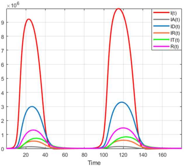
Numerical visualization of COVID-19 model for $\alpha =0.85$

Figure 28.

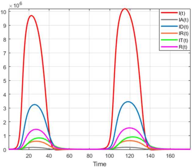
Numerical visualization of COVID-19 model for $\alpha =0.91$

Figure 29.

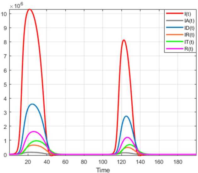
Numerical visualization of COVID-19 model for $\alpha =0.76$

Figure 30.

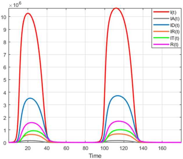
Numerical visualization of COVID-19 model for $\alpha =0.90$, $\beta =0.85$

Figure 31.

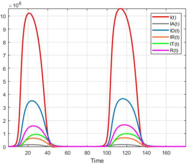
Numerical visualization of COVID-19 model for $\alpha =0.95$, $\beta =0.95$

Figure 32.

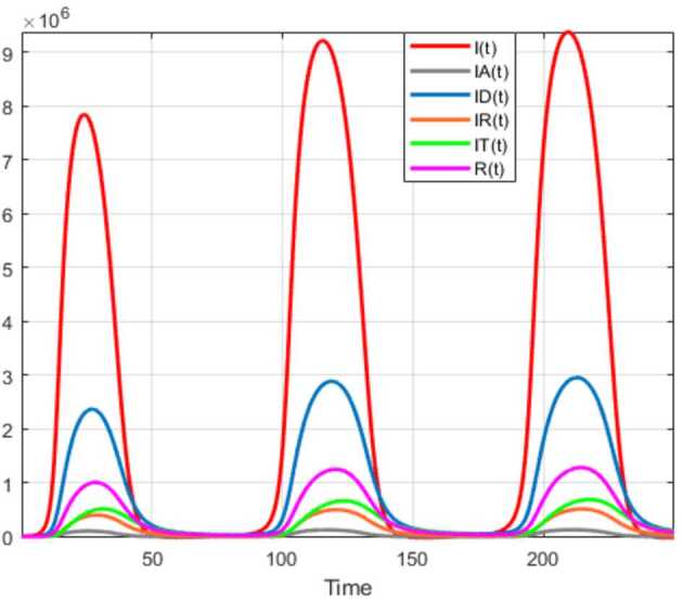
Numerical visualization of COVID-19 model for $\alpha =0.72$

Figure 33.

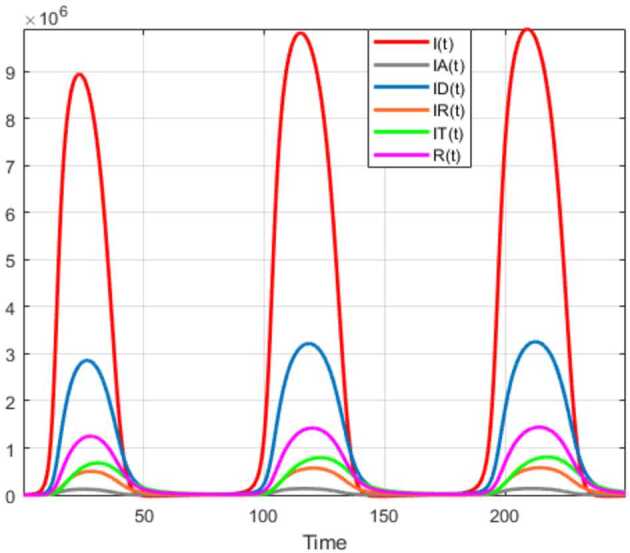
Numerical visualization of COVID-19 model for $\alpha =0.82$

Figure 34.

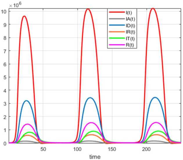
Numerical visualization of COVID-19 model for $\alpha =0.90$

Figure 35.

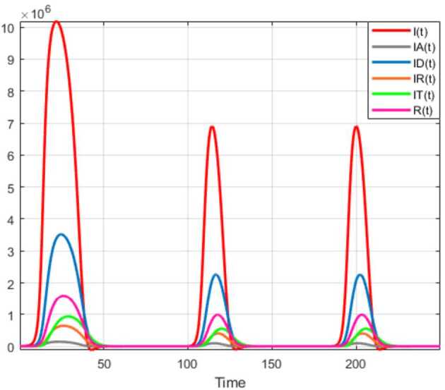
Numerical visualization of COVID-19 model for $\alpha =1$

Figure 36.

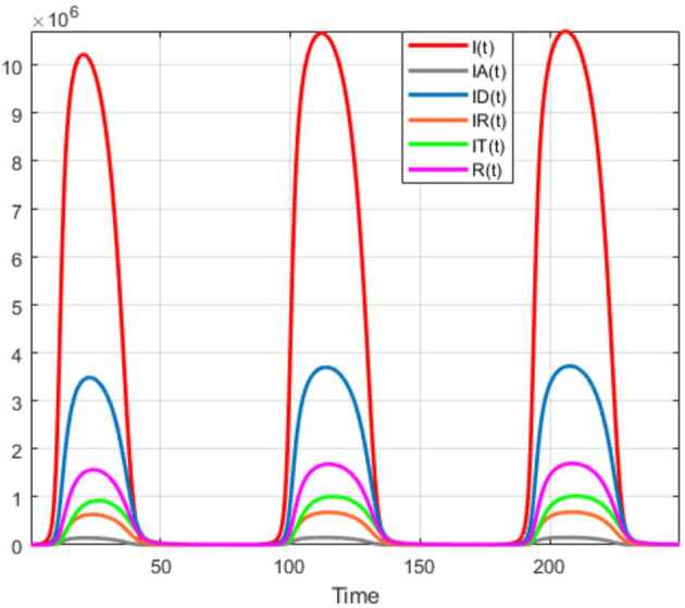
Numerical visualization of COVID-19 model for $\alpha =0.89$, $\beta =0.85$

Figure 26.

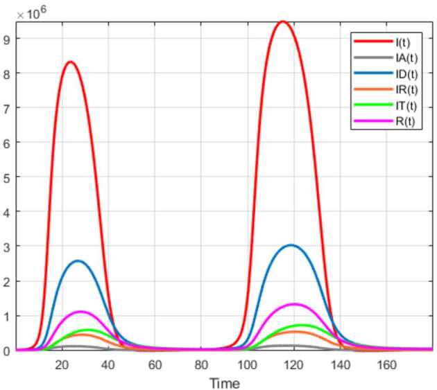
Numerical visualization of COVID-19 model for $\alpha =0.76$

Figure 37.

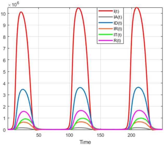
Numerical visualization of COVID-19 model for $\alpha =0.95$, $\beta =0.97$

Likelihood with hyper-Poisson distribution

Using the suggested numerical model, we obtain the approximate solution $(S^{\ast }(t),I^{\ast }(t),I_A^{\ast }(t),I_D^{\ast }(t),I_R^{\ast }(t),I_T^{\ast }(t),R^{\ast }(t),D^{\ast }(t),V^{\ast }(t))$. We are more interested in $I^{\ast }(t)$, $R^{\ast }(t)$, and $D^{\ast }(t)$ and the approximate solution I, R, D because we have the collected data $z_I^t$, $z_R^t$, $z_D^t$ which represent the number of infections, recovered, and deaths daily. We assume that such follow hyper-Poisson distribution with parameters. The hyper-Poisson distribution is given as follows:

$$P(X=k)=\frac{\mathrm{\Gamma }(\beta )}{\mathrm{\Gamma }(k+\beta )\mathrm{\Phi }(1,\beta ,\lambda )},\lambda >0,k=0,1,2,\dots ,n,$$ 145

where

$$\mathrm{\Phi }(1,\beta ,\lambda )=\sum _{k=0}^{\mathrm{\infty }}\frac{{(1)}_k{\lambda }^k}{{(\beta )}_{k}k!},{(\beta )}_k=\beta (\beta +1)\cdots (\beta +k)$$ 146

${\mathrm{\Omega }}_{{}^{″}}$ with parameters $k_1$, $k_2$, $k_3$

$$\begin{array}{c}{k}_1={\mathrm{\Omega }}_1{I}^{\ast }(t),\hfill \\ k_2={\mathrm{\Omega }}_2{R}^{\ast }(t),\hfill \\ k_3={\mathrm{\Omega }}_3{D}^{\ast }(t)\hfill \end{array}$$ 147

and

$$\begin{array}{c}{z}_I^t\sim HP(k_1={\mathrm{\Omega }}_1{I}^{\ast }(t)),\hfill \\ z_R^t\sim HP(k_2={\mathrm{\Omega }}_2{R}^{\ast }(t)),\hfill \\ z_D^t\sim HP(k_3={\mathrm{\Omega }}_3{D}^{\ast }(t)).\hfill \end{array}$$ 148

Here, the parameters ${\mathrm{\Omega }}_1$, ${\mathrm{\Omega }}_2$, and ${\mathrm{\Omega }}_3$ are a combination of collection accuracy and detectability of infected, recovered, and dead. Thus the likelihood function is defined as follows:

$$\begin{array}{c}L(k_1)=\prod _{t=0}^{n}g(z_I^t/k_1),\hfill \\ L(k_2)=\prod _{t=0}^{n}g(z_R^t/k_2),\hfill \\ L(k_3)=\prod _{t=0}^{n}g(z_D^t/k_3).\hfill \end{array}$$ 149

Thus

$$\begin{array}{c}L(k_1)=\prod _{t=0}^n\frac{\mathrm{\Gamma }(\beta ){\lambda }^{z_I^t}}{\mathrm{\Gamma }(z_I^t+\beta )\mathrm{\Phi }(1,\beta ,\lambda )},\hfill \\ L(k_2)=\prod _{t=0}^n\frac{\mathrm{\Gamma }(\beta ){\lambda }^{z_R^t}}{\mathrm{\Gamma }(z_R^t+\beta )\mathrm{\Phi }(1,\beta ,\lambda )},\hfill \\ L(k_3)=\prod _{t=0}^n\frac{\mathrm{\Gamma }(\beta ){\lambda }^{z_D^t}}{\mathrm{\Gamma }(z_D^t+\beta )\mathrm{\Phi }(1,\beta ,\lambda )}.\hfill \end{array}$$ 150

Without loss of generality, we consider $L(k_1)$:

$$\begin{array}{rl}logL(k_1)& =\sum _{t=0}^{n}log\frac{\mathrm{\Gamma }(\beta ){\lambda }^{z_I^t}}{\mathrm{\Gamma }(z_I^t+\beta )\mathrm{\Phi }(1,\beta ,\lambda )}\\ & =\sum _{t=0}^n[log\mathrm{\Gamma }(\beta )+z_I^{t}log\left({\mathrm{\Omega }}_1{I}^{\ast }\right)-log\mathrm{\Gamma }(z_I^t+\beta )-log\mathrm{\Phi }(1,\beta ,{\mathrm{\Omega }}_1{I}^{\ast })]\end{array}$$ 151

and

$$\begin{array}{rl}\frac{\partial logL(k_1)}{\partial z_I^t}& =\sum _{t=0}^{n}log({\mathrm{\Omega }}_1)+\sum _{t=0}^{n}log\left(I^{\ast }\right)-\sum _{t=0}^n\frac{(\mathrm{\Gamma }(z_I^t+\beta ))\prime }{\mathrm{\Gamma }(z_I^t+\beta )}\\ & =n[log({\mathrm{\Omega }}_1)+log\left(I^{\ast }\right)]-\sum _{t=0}^n\frac{(\mathrm{\Gamma }(z_I^t+\beta ))\prime }{\mathrm{\Gamma }(z_I^t+\beta )}\\ & =nlog\left({\mathrm{\Omega }}_1{I}^{\ast }\right)-\sum _{t=0}^n\frac{(\mathrm{\Gamma }(z_I^t+\beta ))\prime }{\mathrm{\Gamma }(z_I^t+\beta )},\end{array}$$ 152

$$\begin{array}{rl}\frac{\partial logL(k_1)}{\partial I^{\ast }}& =n{z}_I^t\frac{I^{\ast }\prime }{I^{\ast }}-\sum _{t=0}^n\frac{\mathrm{\Phi }(1,\beta ,{\mathrm{\Omega }}_1{I}^{\ast })\prime }{\mathrm{\Phi }(1,\beta ,{\mathrm{\Omega }}_1{I}^{\ast })}\\ & =n{z}_I^t\frac{I^{\ast }\prime }{I^{\ast }}-n\frac{\mathrm{\Phi }(1,\beta ,{\mathrm{\Omega }}_1{I}^{\ast })\prime }{\mathrm{\Phi }(1,\beta ,{\mathrm{\Omega }}_1{I}^{\ast })},\end{array}$$ 153

$$\begin{array}{rl}\frac{\partial logL(k_1)}{\partial {\mathrm{\Omega }}_1}& =n{z}_I^t\frac{{\mathrm{\Omega }}_1\prime }{{\mathrm{\Omega }}_1}-n\frac{\mathrm{\Phi }(1,\beta ,{\mathrm{\Omega }}_1{I}^{\ast })\prime }{\mathrm{\Phi }(1,\beta ,{\mathrm{\Omega }}_1{I}^{\ast })}\\ & =-n\frac{\mathrm{\Phi }(1,\beta ,{\mathrm{\Omega }}_1{I}^{\ast })\prime }{\mathrm{\Phi }(1,\beta ,{\mathrm{\Omega }}_1{I}^{\ast })},\end{array}$$ 154

$$\begin{array}{rl}L(k_2)& =\sum _{t=0}^{n}log\frac{\mathrm{\Gamma }(\beta ){\lambda }^{z_R^t}}{\mathrm{\Gamma }(z_R^t+\beta )\mathrm{\Phi }(1,\beta ,\lambda )}\\ & =\sum _{t=0}^n[log\mathrm{\Gamma }(\beta )+z_R^{t}log\lambda -log\mathrm{\Gamma }(z_R^t+\beta )-log\mathrm{\Phi }(1,\beta ,\lambda )],\end{array}$$ 155

$$\begin{array}{rl}\frac{\partial logL(k_2)}{\partial z_R^t}& =\sum _{t=0}^{n}log({\mathrm{\Omega }}_2)+\sum _{t=0}^{n}log\left(R^{\ast }\right)-\sum _{t=0}^n\frac{(\mathrm{\Gamma }(z_R^t+\beta ))\prime }{\mathrm{\Gamma }(z_R^t+\beta )}\\ & =n[log({\mathrm{\Omega }}_2)+log\left(R^{\ast }\right)]-\sum _{t=0}^n\frac{(\mathrm{\Gamma }(z_R^t+\beta ))\prime }{\mathrm{\Gamma }(z_R^t+\beta )}\\ & =nlog\left({\mathrm{\Omega }}_2{R}^{\ast }\right)-\sum _{t=0}^n\frac{(\mathrm{\Gamma }(z_R^t+\beta ))\prime }{\mathrm{\Gamma }(z_R^t+\beta )},\end{array}$$ 156

$$\begin{array}{rl}\frac{\partial logL(k_2)}{\partial R^{\ast }}& =n{z}_R^t\frac{R^{\ast }\prime }{R^{\ast }}-\sum _{t=0}^n\frac{\mathrm{\Phi }(1,\beta ,{\mathrm{\Omega }}_2{R}^{\ast })\prime }{\mathrm{\Phi }(1,\beta ,{\mathrm{\Omega }}_2{R}^{\ast })}\\ & =n{z}_R^t\frac{R^{\ast }\prime }{R^{\ast }}-n\frac{\mathrm{\Phi }(1,\beta ,{\mathrm{\Omega }}_2{R}^{\ast })\prime }{\mathrm{\Phi }(1,\beta ,{\mathrm{\Omega }}_2{R}^{\ast })},\end{array}$$ 157

$$\begin{array}{rl}\frac{\partial logL(k_2)}{\partial {\mathrm{\Omega }}_2}& =n{z}_R^t\frac{{\mathrm{\Omega }}_2\prime }{{\mathrm{\Omega }}_2}-n\frac{\mathrm{\Phi }(1,\beta ,{\mathrm{\Omega }}_2{R}^{\ast })\prime }{\mathrm{\Phi }(1,\beta ,{\mathrm{\Omega }}_2{R}^{\ast })}\\ & =-n\frac{\mathrm{\Phi }(1,\beta ,{\mathrm{\Omega }}_2{R}^{\ast })\prime }{\mathrm{\Phi }(1,\beta ,{\mathrm{\Omega }}_2{R}^{\ast })},\end{array}$$ 158

$$\begin{array}{rl}L(k_3)& =\sum _{t=0}^{n}log\frac{\mathrm{\Gamma }(\beta ){\lambda }^{z_D^t}}{\mathrm{\Gamma }(z_D^t+\beta )\mathrm{\Phi }(1,\beta ,\lambda )}\\ & =\sum _{t=0}^n[log\mathrm{\Gamma }(\beta )+z_D^{t}log\lambda -log\mathrm{\Gamma }(z_D^t+\beta )-log\mathrm{\Phi }(1,\beta ,\lambda )],\end{array}$$ 159

$$\begin{array}{rl}\frac{\partial logL(k_3)}{\partial z_D^t}& =\sum _{t=0}^{n}log({\mathrm{\Omega }}_3)+\sum _{t=0}^{n}log\left(D^{\ast }\right)-\sum _{t=0}^n\frac{(\mathrm{\Gamma }(z_D^t+\beta ))\prime }{\mathrm{\Gamma }(z_D^t+\beta )}\\ & =n[log({\mathrm{\Omega }}_3)+log\left(D^{\ast }\right)]-\sum _{t=0}^n\frac{(\mathrm{\Gamma }(z_D^t+\beta ))\prime }{\mathrm{\Gamma }(z_D^t+\beta )}\\ & =nlog\left({\mathrm{\Omega }}_3{D}^{\ast }\right)-\sum _{t=0}^n\frac{(\mathrm{\Gamma }(z_D^t+\beta ))\prime }{\mathrm{\Gamma }(z_D^t+\beta )},\end{array}$$ 160

$$\begin{array}{rl}\frac{\partial logL(k_3)}{\partial R^{\ast }}& =n{z}_D^t\frac{D^{\ast }\prime }{D^{\ast }}-\sum _{t=0}^n\frac{\mathrm{\Phi }(1,\beta ,{\mathrm{\Omega }}_3{D}^{\ast })\prime }{\mathrm{\Phi }(1,\beta ,{\mathrm{\Omega }}_3{D}^{\ast })}\\ & =n{z}_D^t\frac{D^{\ast }\prime }{D^{\ast }}-n\frac{\mathrm{\Phi }(1,\beta ,{\mathrm{\Omega }}_3{D}^{\ast })\prime }{\mathrm{\Phi }(1,\beta ,{\mathrm{\Omega }}_3{D}^{\ast })},\end{array}$$ 161

$$\begin{array}{rl}\frac{\partial logL(k_3)}{\partial {\mathrm{\Omega }}_3}& =n{z}_D^t\frac{{\mathrm{\Omega }}_3\prime }{{\mathrm{\Omega }}_3}-n\frac{\mathrm{\Phi }(1,\beta ,{\mathrm{\Omega }}_3{D}^{\ast })\prime }{\mathrm{\Phi }(1,\beta ,{\mathrm{\Omega }}_3{D}^{\ast })}\\ & =-n\frac{\mathrm{\Phi }(1,\beta ,{\mathrm{\Omega }}_3{D}^{\ast })\prime }{\mathrm{\Phi }(1,\beta ,{\mathrm{\Omega }}_3{D}^{\ast })}.\end{array}$$ 162

Likelihood with Weibull distribution

We will do the same routine for the Weibull distribution known as

$$P(X=k)=\frac{k}{\alpha }{\left(\frac{\lambda }{\alpha }\right)}^{k-1}exp{(-\lambda /\alpha )}^k,\lambda ,\alpha >0,k=0,1,2,\dots ,n,$$ 163

Ω with parameters $k_1$, $k_2$, $k_3$

$$\begin{array}{c}{k}_1={\mathrm{\Omega }}_1{I}^{\ast }(t),\hfill \\ k_2={\mathrm{\Omega }}_2{R}^{\ast }(t),\hfill \\ k_3={\mathrm{\Omega }}_3{D}^{\ast }(t)\hfill \end{array}$$ 164

and

$$\begin{array}{c}{\epsilon }_I^t\sim W(k_1={\mathrm{\Omega }}_1{I}^{\ast }(t)),\hfill \\ {\epsilon }_R^t\sim W(k_2={\mathrm{\Omega }}_2{R}^{\ast }(t)),\hfill \\ {\epsilon }_D^t\sim W(k_3={\mathrm{\Omega }}_3{D}^{\ast }(t)).\hfill \end{array}$$ 165

Thus the likelihood function is given by

$$\begin{array}{c}L(k_1)=\prod _{t=0}^{n}W({\epsilon }_I^t/k_1),\hfill \\ L(k_2)=\prod _{t=0}^{n}W({\epsilon }_R^t/k_2),\hfill \\ L(k_3)=\prod _{t=0}^{n}W({\epsilon }_D^t/k_3).\hfill \end{array}$$ 166

Thus

$$\begin{array}{c}L(k_1)=\prod _{t=0}^n\frac{{\epsilon }_I^t}{\alpha }{\left(\frac{\lambda }{\alpha }\right)}^{{\epsilon }_I^t-1}exp{(-\lambda /\alpha )}^{{\epsilon }_I^t},\hfill \\ L(k_2)=\prod _{t=0}^n\frac{{\epsilon }_R^t}{\alpha }{\left(\frac{\lambda }{\alpha }\right)}^{{\epsilon }_R^t-1}exp{(-\lambda /\alpha )}^{{\epsilon }_R^t},\hfill \\ L(k_3)=\prod _{t=0}^n\frac{{\epsilon }_D^t}{\alpha }{\left(\frac{\lambda }{\alpha }\right)}^{{\epsilon }_D^t-1}exp{(-\lambda /\alpha )}^{{\epsilon }_D^t}.\hfill \end{array}$$ 167

Without loss of generality, we consider $L(k_1)$:

$$\begin{array}{rcl}logL(k_1)& =& \sum _{t=0}^{n}log[\frac{{\epsilon }_I^t}{\alpha }{\left(\frac{{\mathrm{\Omega }}_1{I}^{\ast }}{\alpha }\right)}^{{\epsilon }_I^t-1}exp{(-{\mathrm{\Omega }}_1{I}^{\ast }/\alpha )}^{{\epsilon }_I^t}]\\ & =& [log{\epsilon }_I^t-log\alpha +({\epsilon }_I^t-1)[log\left({\mathrm{\Omega }}_1{I}^{\ast }\right)-log\alpha ]-{\epsilon }_I^t(-{\mathrm{\Omega }}_1{I}^{\ast }/\alpha )]\end{array}$$ 168

and

$$\begin{array}{rl}\frac{\partial logL(k_1)}{\partial {\epsilon }_I^t}& =\sum _{t=0}^n\frac{{\epsilon }_I^t\prime }{{\epsilon }_I^t}+\sum _{t=0}^n[log\left({\mathrm{\Omega }}_1{I}^{\ast }\right)-log\alpha ]-\sum _{t=0}^n(-{\mathrm{\Omega }}_1{I}^{\ast }/\alpha )\\ & =n\frac{{\epsilon }_I^t\prime }{{\epsilon }_I^t}+n[log\left({\mathrm{\Omega }}_1{I}^{\ast }\right)-log\alpha ]+n({\mathrm{\Omega }}_1{I}^{\ast }/\alpha ),\end{array}$$ 169

$$\begin{array}{rl}\frac{\partial logL(k_1)}{\partial I^{\ast }}& =n({\epsilon }_I^t-1)\frac{I^{\ast }\prime }{I^{\ast }}-\sum _{t=0}^n\frac{(-{\mathrm{\Omega }}_1{I}^{\ast }/\alpha )\prime }{(-{\mathrm{\Omega }}_1{I}^{\ast }/\alpha )}\\ & =n({\epsilon }_I^t-1)\frac{I^{\ast }\prime }{I^{\ast }}-n\frac{(-{\mathrm{\Omega }}_1{I}^{\ast }/\alpha )\prime }{(-{\mathrm{\Omega }}_1{I}^{\ast }/\alpha )},\end{array}$$ 170

$$\begin{array}{rl}\frac{\partial logL(k_1)}{\partial {\mathrm{\Omega }}_1}& =n({\epsilon }_I^t-1)\frac{{\mathrm{\Omega }}_1\prime }{{\mathrm{\Omega }}_1}-n\frac{(-{\mathrm{\Omega }}_1{I}^{\ast }/\alpha )\prime }{(-{\mathrm{\Omega }}_1{I}^{\ast }/\alpha )}\\ & =-n\frac{(-{\mathrm{\Omega }}_1{I}^{\ast }/\alpha )\prime }{(-{\mathrm{\Omega }}_1{I}^{\ast }/\alpha )},\end{array}$$ 171

$$\begin{array}{rl}logL(k_2)& =\sum _{t=0}^{n}log[\frac{{\epsilon }_R^t}{\alpha }{\left(\frac{{\mathrm{\Omega }}_2{I}^{\ast }}{\alpha }\right)}^{{\epsilon }_R^t-1}exp{(-{\mathrm{\Omega }}_2{R}^{\ast }/\alpha )}^{{\epsilon }_I^t}]\\ & =[log{\epsilon }_R^t-log\alpha +({\epsilon }_R^t-1)[log\left({\mathrm{\Omega }}_2{R}^{\ast }\right)-log\alpha ]-{\epsilon }_R^t(-{\mathrm{\Omega }}_2{R}^{\ast }/\alpha )]\end{array}$$ 172

and

$$\begin{array}{rl}\frac{\partial logL(k_2)}{\partial {\epsilon }_R^t}& =\sum _{t=0}^n\frac{{\epsilon }_R^t\prime }{{\epsilon }_R^t}+\sum _{t=0}^n[log\left({\mathrm{\Omega }}_2{R}^{\ast }\right)-log\alpha ]-\sum _{t=0}^n(-{\mathrm{\Omega }}_2{R}^{\ast }/\alpha )\\ & =n\frac{{\epsilon }_R^t\prime }{{\epsilon }_R^t}+n[log\left({\mathrm{\Omega }}_2{R}^{\ast }\right)-log\alpha ]+n(-{\mathrm{\Omega }}_2{R}^{\ast }/\alpha ),\end{array}$$ 173

$$\begin{array}{rl}\frac{\partial logL(k_2)}{\partial R^{\ast }}& =n({\epsilon }_R^t-1)\frac{R^{\ast }\prime }{R^{\ast }}-\sum _{t=0}^n\frac{(-{\mathrm{\Omega }}_2{R}^{\ast }/\alpha )\prime }{(-{\mathrm{\Omega }}_2{R}^{\ast }/\alpha )}\\ & =n({\epsilon }_R^t-1)\frac{R^{\ast }\prime }{R^{\ast }}-n\frac{(-{\mathrm{\Omega }}_2{R}^{\ast }/\alpha )\prime }{(-{\mathrm{\Omega }}_2{R}^{\ast }/\alpha )},\end{array}$$ 174

$$\begin{array}{rl}\frac{\partial logL(k_2)}{\partial {\mathrm{\Omega }}_2}& =n({\epsilon }_R^t-1)\frac{{\mathrm{\Omega }}_2\prime }{{\mathrm{\Omega }}_2}-n\frac{(-{\mathrm{\Omega }}_2{R}^{\ast }/\alpha )\prime }{(-{\mathrm{\Omega }}_2{R}^{\ast }/\alpha )}\\ & =-n\frac{(-{\mathrm{\Omega }}_2{R}^{\ast }/\alpha )\prime }{(-{\mathrm{\Omega }}_2{R}^{\ast }/\alpha )},\end{array}$$ 175

$$\begin{array}{rl}logL(k_3)& =\sum _{t=0}^{n}log[\frac{{\epsilon }_D^t}{\alpha }{\left(\frac{{\mathrm{\Omega }}_3{D}^{\ast }}{\alpha }\right)}^{{\epsilon }_D^t-1}exp{(-{\mathrm{\Omega }}_3{D}^{\ast }/\alpha )}^{{\epsilon }_D^t}]\\ & =[log{\epsilon }_D^t-log\alpha +({\epsilon }_D^t-1)[log\left({\mathrm{\Omega }}_3{D}^{\ast }\right)-log\alpha ]-{\epsilon }_D^t(-{\mathrm{\Omega }}_3{D}^{\ast }/\alpha )]\end{array}$$ 176

and

$$\begin{array}{rl}\frac{\partial logL(k_3)}{\partial {\epsilon }_D^t}& =\sum _{t=0}^n\frac{{\epsilon }_D^t\prime }{{\epsilon }_D^t}+\sum _{t=0}^n[log\left({\mathrm{\Omega }}_3{D}^{\ast }\right)-log\alpha ]-\sum _{t=0}^n(-{\mathrm{\Omega }}_3{D}^{\ast }/\alpha )\\ & =n\frac{{\epsilon }_D^t\prime }{{\epsilon }_D^t}+n[log\left({\mathrm{\Omega }}_3{R}^{\ast }\right)-log\alpha ]+n(-{\mathrm{\Omega }}_3{D}^{\ast }/\alpha ),\end{array}$$ 177

$$\begin{array}{rl}\frac{\partial logL(k_3)}{\partial D^{\ast }}& =n({\epsilon }_D^t-1)\frac{D^{\ast }\prime }{D^{\ast }}-\sum _{t=0}^n\frac{(-{\mathrm{\Omega }}_3{D}^{\ast }/\alpha )\prime }{(-{\mathrm{\Omega }}_3{D}^{\ast }/\alpha )}\\ & =n({\epsilon }_I^t-1)\frac{D^{\ast }\prime }{D^{\ast }}-n\frac{(-{\mathrm{\Omega }}_3{D}^{\ast }/\alpha )\prime }{(-{\mathrm{\Omega }}_3{D}^{\ast }/\alpha )},\end{array}$$ 178

$$\begin{array}{rl}\frac{\partial logL(k_1)}{\partial {\mathrm{\Omega }}_1}& =n({\epsilon }_D^t-1)\frac{{\mathrm{\Omega }}_3\prime }{{\mathrm{\Omega }}_3}-n\frac{(-{\mathrm{\Omega }}_3{D}^{\ast }/\alpha )\prime }{(-{\mathrm{\Omega }}_3{D}^{\ast }/\alpha )}\\ & =-n\frac{(-{\mathrm{\Omega }}_3{D}^{\ast }/\alpha )\prime }{(-{\mathrm{\Omega }}_3{D}^{\ast }/\alpha )}.\end{array}$$ 179

Likelihood with Mittag-Leffler distribution

Finally, we shall use the Mittag-Leffler distribution for similar processes. The Mittag-Leffler distribution is defined by

$$P(X=k)=\frac{{\lambda }^k}{\mathrm{\Gamma }(\alpha k+\beta )E_{\alpha ,\beta }(\lambda )},\lambda >0,k=0,1,2,\dots ,n,$$ 180

where

$$E_{\alpha ,\beta }(\lambda )=\sum _{k=0}^{\mathrm{\infty }}\frac{{\lambda }^k}{\mathrm{\Gamma }(\alpha k+\beta )}.$$ 181

${\mathrm{\Omega }}_i$, $i=1,2,3$ with parameters $k_1$, $k_2$, $k_3$

$$\begin{array}{c}{k}_1={\mathrm{\Omega }}_1{I}^{\ast }(t),\hfill \\ k_2={\mathrm{\Omega }}_2{R}^{\ast }(t),\hfill \\ k_3={\mathrm{\Omega }}_3{D}^{\ast }(t)\hfill \end{array}$$ 182

and

$$\begin{array}{c}{\epsilon }_I^t\sim ML(k_1={\mathrm{\Omega }}_1{I}^{\ast }(t)),\hfill \\ {\epsilon }_R^t\sim ML(k_2={\mathrm{\Omega }}_2{R}^{\ast }(t)),\hfill \\ {\epsilon }_D^t\sim ML(k_3={\mathrm{\Omega }}_3{D}^{\ast }(t)).\hfill \end{array}$$ 183

Thus the likelihood function is written as

$$\begin{array}{c}L(k_1)=\prod _{t=0}^{n}ML({\epsilon }_I^t/k_1),\hfill \\ L(k_2)=\prod _{t=0}^{n}ML({\epsilon }_R^t/k_2),\hfill \\ L(k_3)=\prod _{t=0}^{n}ML({\epsilon }_D^t/k_3).\hfill \end{array}$$ 184

Thus

$$\begin{array}{c}L(k_1)=\prod _{t=0}^n\frac{{\lambda }^{{\epsilon }_I^t}}{\mathrm{\Gamma }(\alpha {\epsilon }_I^t+\beta )E_{\alpha ,\beta }(\lambda )},\hfill \\ L(k_2)=\prod _{t=0}^n\frac{{\lambda }^{{\epsilon }_R^t}}{\mathrm{\Gamma }(\alpha {\epsilon }_R^t+\beta )E_{\alpha ,\beta }(\lambda )},\hfill \\ L(k_3)=\prod _{t=0}^n\frac{{\lambda }^{{\epsilon }_D^t}}{\mathrm{\Gamma }(\alpha {\epsilon }_D^t+\beta )E_{\alpha ,\beta }(\lambda )}.\hfill \end{array}$$ 185

We write $L(k_1)$:

$$\begin{array}{rcl}logL(k_1)& =& log\frac{{\lambda }^{{\epsilon }_I^t}}{\mathrm{\Gamma }(\alpha {\epsilon }_I^t+\beta )E_{\alpha ,\beta }(\lambda )}\\ & =& \sum _{t=0}^n[{\epsilon }_I^{t}log\left({\mathrm{\Omega }}_1{I}^{\ast }\right)-log\mathrm{\Gamma }(\alpha {\epsilon }_I^t+\beta )-log{E}_{\alpha ,\beta }\left({\mathrm{\Omega }}_1{I}^{\ast }\right)]\end{array}$$ 186

and

$$\begin{array}{rl}\frac{\partial logL(k_1)}{\partial {\epsilon }_I^t}& =\sum _{t=0}^{n}log({\mathrm{\Omega }}_1)+\sum _{t=0}^{n}log\left(I^{\ast }\right)-\sum _{t=0}^n\frac{(\mathrm{\Gamma }(\alpha {\epsilon }_I^t+\beta ))\prime }{\mathrm{\Gamma }(\alpha {\epsilon }_I^t+\beta )}\\ & =n[log({\mathrm{\Omega }}_1)+log\left(I^{\ast }\right)]-\sum _{t=0}^n\frac{(\mathrm{\Gamma }(\alpha {\epsilon }_I^t+\beta ))\prime }{\mathrm{\Gamma }(\alpha {\epsilon }_I^t+\beta )}\\ & =nlog\left({\mathrm{\Omega }}_1{I}^{\ast }\right)-\sum _{t=0}^n\frac{(\mathrm{\Gamma }(\alpha {\epsilon }_I^t+\beta ))\prime }{\mathrm{\Gamma }(\alpha {\epsilon }_I^t+\beta )},\end{array}$$ 187

$$\begin{array}{rl}\frac{\partial logL(k_1)}{\partial I^{\ast }}& =n{\epsilon }_I^t\frac{I^{\ast }\prime }{I^{\ast }}-\sum _{t=0}^n\frac{E_{\alpha ,\beta }({\mathrm{\Omega }}_1{I}^{\ast })\prime }{E_{\alpha ,\beta }({\mathrm{\Omega }}_1{I}^{\ast })}\\ & =n{\epsilon }_I^t\frac{I^{\ast }\prime }{I^{\ast }}-n\frac{E_{\alpha ,\beta }({\mathrm{\Omega }}_1{I}^{\ast })\prime }{E_{\alpha ,\beta }({\mathrm{\Omega }}_1{I}^{\ast })},\end{array}$$ 188

$$\begin{array}{rl}\frac{\partial logL(k_1)}{\partial {\mathrm{\Omega }}_1}& =n{\epsilon }_I^t\frac{{\mathrm{\Omega }}_1\prime }{{\mathrm{\Omega }}_1}-n\frac{E_{\alpha ,\beta }({\mathrm{\Omega }}_1{I}^{\ast })\prime }{E_{\alpha ,\beta }({\mathrm{\Omega }}_1{I}^{\ast })}\\ & =-n\frac{E_{\alpha ,\beta }({\mathrm{\Omega }}_1{I}^{\ast })\prime }{E_{\alpha ,\beta }({\mathrm{\Omega }}_1{I}^{\ast })}.\end{array}$$ 189

With the same routine,

$$\begin{array}{rcl}logL(k_2)& =& \sum _{t=0}^{n}log\frac{{\lambda }^{{\epsilon }_R^t}}{\mathrm{\Gamma }(\alpha {\epsilon }_I^t+\beta )E_{\alpha ,\beta }(\lambda )}\\ & =& \sum _{t=0}^n[{\epsilon }_R^{t}log\left({\mathrm{\Omega }}_1{R}^{\ast }\right)-log\mathrm{\Gamma }(\alpha {\epsilon }_R^t+\beta )-log{E}_{\alpha ,\beta }\left({\mathrm{\Omega }}_2{R}^{\ast }\right)]\end{array}$$ 190

and

$$\begin{array}{rl}\frac{\partial logL(k_2)}{\partial {\epsilon }_R^t}& =\sum _{t=0}^{n}log({\mathrm{\Omega }}_2)+\sum _{t=0}^{n}log\left(R^{\ast }\right)-\sum _{t=0}^n\frac{(\mathrm{\Gamma }(\alpha {\epsilon }_R^t+\beta ))\prime }{\mathrm{\Gamma }(\alpha {\epsilon }_R^t+\beta )}\\ & =n[log({\mathrm{\Omega }}_2)+log\left(R^{\ast }\right)]-\sum _{t=0}^n\frac{(\mathrm{\Gamma }(\alpha {\epsilon }_R^t+\beta ))\prime }{\mathrm{\Gamma }(\alpha {\epsilon }_R^t+\beta )}\\ & =nlog\left({\mathrm{\Omega }}_2{R}^{\ast }\right)-\sum _{t=0}^n\frac{(\mathrm{\Gamma }(\alpha {\epsilon }_R^t+\beta ))\prime }{\mathrm{\Gamma }(\alpha {\epsilon }_R^t+\beta )},\end{array}$$ 191

$$\begin{array}{rl}\frac{\partial logL(k_2)}{\partial R^{\ast }}& =n{\epsilon }_R^t\frac{R^{\ast }\prime }{R^{\ast }}-\sum _{t=0}^n\frac{E_{\alpha ,\beta }({\mathrm{\Omega }}_2{R}^{\ast })\prime }{E_{\alpha ,\beta }({\mathrm{\Omega }}_2{R}^{\ast })}\\ & =n{\epsilon }_I^t\frac{R^{\ast }\prime }{R^{\ast }}-n\frac{E_{\alpha ,\beta }({\mathrm{\Omega }}_2{R}^{\ast })\prime }{E_{\alpha ,\beta }({\mathrm{\Omega }}_2{R}^{\ast })},\end{array}$$ 192

$$\begin{array}{rl}\frac{\partial logL(k_2)}{\partial {\mathrm{\Omega }}_2}& =n{\epsilon }_R^t\frac{{\mathrm{\Omega }}_2\prime }{{\mathrm{\Omega }}_2}-n\frac{E_{\alpha ,\beta }({\mathrm{\Omega }}_2{R}^{\ast })\prime }{E_{\alpha ,\beta }({\mathrm{\Omega }}_2{R}^{\ast })}\\ & =-n\frac{E_{\alpha ,\beta }({\mathrm{\Omega }}_2{R}^{\ast })\prime }{E_{\alpha ,\beta }({\mathrm{\Omega }}_2{R}^{\ast })}\end{array}$$ 193

and

$$\begin{array}{rcl}logL(k_3)& =& \sum _{t=0}^{n}log\frac{{\lambda }^{{\epsilon }_D^t}}{\mathrm{\Gamma }(\alpha {\epsilon }_D^t+\beta )E_{\alpha ,\beta }(\lambda )}\\ & =& \sum _{t=0}^n[{\epsilon }_D^{t}log\left({\mathrm{\Omega }}_3{D}^{\ast }\right)-log\mathrm{\Gamma }(\alpha {\epsilon }_D^t+\beta )-log{E}_{\alpha ,\beta }\left({\mathrm{\Omega }}_3{D}^{\ast }\right)]\end{array}$$ 194

and

$$\begin{array}{rl}\frac{\partial logL(k_1)}{\partial {\epsilon }_I^t}& =\sum _{t=0}^{n}log({\mathrm{\Omega }}_3)+\sum _{t=0}^{n}log\left(D^{\ast }\right)-\sum _{t=0}^n\frac{(\mathrm{\Gamma }(\alpha {\epsilon }_D^t+\beta ))\prime }{\mathrm{\Gamma }(\alpha {\epsilon }_D^t+\beta )}\\ & =n[log({\mathrm{\Omega }}_3)+log\left(D^{\ast }\right)]-\sum _{t=0}^n\frac{(\mathrm{\Gamma }(\alpha {\epsilon }_D^t+\beta ))\prime }{\mathrm{\Gamma }(\alpha {\epsilon }_D^t+\beta )}\\ & =nlog\left({\mathrm{\Omega }}_3{D}^{\ast }\right)-\sum _{t=0}^n\frac{(\mathrm{\Gamma }(\alpha {\epsilon }_D^t+\beta ))\prime }{\mathrm{\Gamma }(\alpha {\epsilon }_D^t+\beta )},\end{array}$$ 195

$$\begin{array}{rl}\frac{\partial logL(k_3)}{\partial D^{\ast }}& =n{\epsilon }_D^t\frac{D^{\ast }\prime }{D^{\ast }}-\sum _{t=0}^n\frac{E_{\alpha ,\beta }({\mathrm{\Omega }}_3{D}^{\ast })\prime }{E_{\alpha ,\beta }({\mathrm{\Omega }}_3{D}^{\ast })}\\ & =n{\epsilon }_D^t\frac{D^{\ast }\prime }{D^{\ast }}-n\frac{E_{\alpha ,\beta }({\mathrm{\Omega }}_3{D}^{\ast })\prime }{E_{\alpha ,\beta }({\mathrm{\Omega }}_3{D}^{\ast })},\end{array}$$ 196

$$\begin{array}{rl}\frac{\partial logL(k_3)}{\partial {\mathrm{\Omega }}_3}& =n{\epsilon }_D^t\frac{{\mathrm{\Omega }}_1\prime }{{\mathrm{\Omega }}_1}-n\frac{E_{\alpha ,\beta }({\mathrm{\Omega }}_3{D}^{\ast })\prime }{E_{\alpha ,\beta }({\mathrm{\Omega }}_3{D}^{\ast })}\\ & =-n\frac{E_{\alpha ,\beta }({\mathrm{\Omega }}_3{D}^{\ast })\prime }{E_{\alpha ,\beta }({\mathrm{\Omega }}_3{D}^{\ast })}.\end{array}$$ 197

Conclusion

Up to date humans have relied on forecasting with the aim to better control their world, or at least to have an asymptotic idea of their future. They have many ways to achieve this, one way is to use the deterministic approach and another is stochastic one. In this work, we presented a comprehensive analysis ranging from stochastic, fractal to differentiation with the aim to predict the future behavior of COVID-19 with cases studied in Africa and Europe. With stochastic approach, we were able to detect a possibility of the second wave of COVID-19 spread in Europe and in Africa, a continuous exponential growth could be possible. We presented an extension of the blancmange function to capture more fractal behaviors, and some examples were presented resembling the COVID-19 spread in various countries in Africa and Europe. A complex and nonlinear mathematical model with wave function was considered and solved numerically with a modified scheme.

Authors’ contributions

All authors have contributed equally in this work. All authors read and approved the final manuscript.

Funding

There is no funding for this paper.

Availability of data and materials

There are no data for this paper.

Competing interests

The authors declare that they have no competing interests.

References

- 1. WHO: Coronavirus disease (Covid-2019) situation reports. https://www.who.int/emergencies/diseases/novel-coronavirus-2019/situation-reports
- 2.https://who.maps.arcgis.com/apps/opsdashboard/index.html#/ead3c6475654481ca51c248d52ab9c61
- 3.Ndaïrou F., Area I., Nieto J.J., Torres D.F.M. Mathematical modeling of Covid-19 transmission dynamics with a case study of Wuhan. Chaos Solitons Fractals. 2020;135:109846. doi: 10.1016/j.chaos.2020.109846. [DOI] [PMC free article] [PubMed] [Google Scholar]
- 4.Khan M.A., Atangana A. Modeling the dynamics of novel coronavirus (2019-nCov) with fractional derivative. Alex. Eng. J. 2020;59(4):2379–2389. doi: 10.1016/j.aej.2020.02.033. [DOI] [Google Scholar]
- 5.Postnikov E.B. Estimation of Covid-19 dynamics “on a back-of-envelope”: does the simplest SIR model provide quantitative parameters and predictions? Chaos Solitons Fractals. 2020;135:109841. doi: 10.1016/j.chaos.2020.109841. [DOI] [PMC free article] [PubMed] [Google Scholar]
- 6.Atangana A., İğret Araz S. Nonlinear equations with global differential and integral operators: existence, uniqueness with application to epidemiology. Results Phys. 2020;20:103593. doi: 10.1016/j.rinp.2020.103593. [DOI] [Google Scholar]
- 7.Jiao J., Liu Z., Cai S. Dynamics of an SEIR model with infectivity in incubation period and homestead-isolation on the susceptible. Appl. Math. Lett. 2020;107:106442. doi: 10.1016/j.aml.2020.106442. [DOI] [PMC free article] [PubMed] [Google Scholar]
- 8. Atangana, A., İğret Araz, S.: Mathematical model of Covid-19 spread in Turkey and South Africa: theory, methods and applications. medRxiv (2020) [DOI] [PMC free article] [PubMed]
- 9.Ivorra B., Ferrández M.R., Vela-Péreza M., Ramos A.M. Mathematical modeling of the spread of the coronavirus disease 2019 (Covid-19) taking into account the undetected infections. The case of China. Commun. Nonlinear Sci. Numer. Simul. 2020;88:105303. doi: 10.1016/j.cnsns.2020.105303. [DOI] [PMC free article] [PubMed] [Google Scholar]
- 10.Rezapour S., Mohammadi H., Jajarmi A. A new mathematical model for Zika virus transmission. Adv. Differ. Equ. 2020;2020:589. doi: 10.1186/s13662-020-03044-7. [DOI] [Google Scholar]
- 11.Atangana A. Modelling the spread of COVID-19 with new fractal-fractional operators: can the lockdown save mankind before vaccination? Chaos Solitons Fractals. 2020;136:109860. doi: 10.1016/j.chaos.2020.109860. [DOI] [PMC free article] [PubMed] [Google Scholar]
- 12.Jajarmi A., Baleanu D. A new iterative method for the numerical solution of high-order nonlinear fractional boundary value problems. Front. Phys. 2020;8:220. doi: 10.3389/fphy.2020.00220. [DOI] [Google Scholar]
- 13.Atangana A., İğret Araz S. Analysis of a Covid-19 model: optimal control, stability and simulations. Alex. Eng. J. 2021;60(1):647–658. doi: 10.1016/j.aej.2020.09.058. [DOI] [Google Scholar]
- 14.Singh S., Parmar K.S., Singh Makkhan S.J., Kaur J., Peshoria S., Kumar J. Study of ARIMA and least square support vector machine (LS-SVM) models for the prediction of SARS-CoV-2 confirmed cases in the most affected countries. Chaos Solitons Fractals. 2020;139:110086. doi: 10.1016/j.chaos.2020.110086. [DOI] [PMC free article] [PubMed] [Google Scholar]
- 15.Barnsley M. Fractals Everywhere. 3. New York: Dover; 2012. [Google Scholar]
- 16.Păcurar C.M., Necula B.R. An analysis of Covid-19 spread based on fractal interpolation and fractal dimension. Chaos Solitons Fractals. 2020;139:110073. doi: 10.1016/j.chaos.2020.110073. [DOI] [PMC free article] [PubMed] [Google Scholar]
- 17.Ovidiu C. An Informal Introduction to Stochastic Calculus with Applications. Singapore: World Scientific; 2015. [Google Scholar]
- 18.Atangana A., Araz S.İ. New Numerical Scheme with Newton Polynomial: Theory, Methods, and Applications. San Diego: Academic Press; 2021. [Google Scholar]
Associated Data
This section collects any data citations, data availability statements, or supplementary materials included in this article.
Data Availability Statement