A compartmental epidemic model incorporating probable cases to model COVID-19 outbreak in regions with limited testing capacity

Abstract

We propose a new compartmental epidemic model taking into account people who have symptoms with no confirmatory laboratory testing (probable cases). We prove well-posedness of the model and provide an explicit expression for the basic reproduction number (${\mathcal{R}}_0$). We use the model together with an extended Kalman filter (EKF) to estimate the time-varying effective reproduction number (${\mathcal{R}}_t$) of COVID-19 in West Java province in Indonesia and the state of Michigan in the USA, where laboratory testing capacities are limited. Based on our estimation, the value of ${\mathcal{R}}_t$ is higher when the probable cases are taken into account. This correction can be used by decision and policy makers when considering re-opening policy and evaluation of public measures.

1. Introduction

Since declared as pandemic by WHO in early of March 2020, the coronavirus disease (COVID-19) has been spread to 216 countries and territories by the end of 2020. At the end of 2020, the virus has infected more than 80 million people (confirmed) and caused more than 1.8 million deaths. Particularly in Indonesia, the number of confirmed positive infection is over 750 thousand cases with over 20 thousand deaths, while in the USA the number of confirmed positive infection is over 20 million cases with over 350 thousand deaths. The pandemic has attracted researchers from different disciplines to model and forecast using different approach, e.g., [1], [2].

In order to prevent and control the outbreak, in early April 2020, the Indonesian government began to conduct Large-Scale Social Restriction (LSSR) at several regions with severe outbreak cases, such as in Jakarta and West Java Province. LSSR includes measures such as closing public places, restricting public transport, and limiting travel to and from restricted regions. This regulation is being controlled by each of the local government. Superspreaders dictate COVID-19 transmission in big cities such as Jakarta and Batam [3]. To assess the duration of LSSR, local government relies on the estimation value of the time-varying effective reproduction number (${\mathcal{R}}_t$) at each region. The government officials use sequential Bayesian method based on the discrete SIR model presented in [4], [5]. The method requires daily confirmed infection data as primarily inputs to estimate ${\mathcal{R}}_t$.

Based on CDC case definitions, however, there are two classifications of COVID-19 case, namely probable cases and confirmed cases [6]. A person can be classified into probable case if he or she

• • meets clinical criteria AND epidemiologic evidence with no confirmatory laboratory testing performed for COVID-19,
• • meets presumptive laboratory evidence AND either clinical criteria OR epidemiologic evidence,
• • meets vital records criteria with no confirmatory laboratory testing performed for COVID-19.

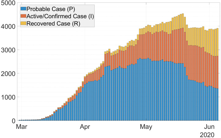
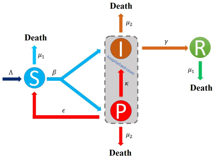
Details regarding clinical criteria, epidemiologic evidence, and vital records criteria can be found in [6]. Probable case is quite similar to Patient under Surveillance (Pasien Dalam Pengawasan or PDP) based on the Indonesian ministry of health. In many provinces in Indonesia, the number of probable cases far exceeded the number of confirmed cases, especially in the beginning of the pandemic. For example, Fig. 1 shows a much larger number of probable cases in West Java province in Indonesia compared to active/confirmed cases. Limited laboratory testing and the lag time between testing and result can be the cause of this situation. Our aim is to estimate the time-varying effective reproduction number ${\mathcal{R}}_t$ by utilizing probable case data together with confirmed case data. To this end, we propose a Susceptible–Probable–Infectious–Recovered (SPIR) model with four compartments as shown in Fig. 2.

Fig. 1.

Stacked-bar of COVID-19 cases in West Java, Indonesia.

Fig. 2.

SPIR model is proposed to model the number of probable case of COVID-19 transmission process.

2. Model description

2.1. Susceptible–probable–infectious–recovered (SPIR) model

The SPIR model consists of four ordinary differential equations (ODEs), describing the evolution of the population in each stage over time, and is given by:

$$\frac{\mathrm{d}S\left(t\right)}{\mathrm{d}t}=\Lambda \left(t\right)-\frac{\beta S\left(t\right)(I\left(t\right)+P\left(t\right))}{N}+\epsilon P\left(t\right)-{\mu }_{1}S\left(t\right),$$ (1)

$$\frac{\mathrm{d}P\left(t\right)}{\mathrm{d}t}=\frac{\beta S\left(t\right)P\left(t\right)}{N}-(\kappa +\epsilon +{\mu }_2)P\left(t\right),$$ (2)

$$\frac{\mathrm{d}I\left(t\right)}{\mathrm{d}t}=\frac{\beta S\left(t\right)I\left(t\right)}{N}+\kappa P\left(t\right)-(\gamma +{\mu }_2)I\left(t\right),$$ (3)

$$\frac{\mathrm{d}R\left(t\right)}{\mathrm{d}t}=\gamma I\left(t\right)-{\mu }_{1}R\left(t\right).$$ (4)

Here, $S$, $P$, $I$, $R$ denote susceptible case, probable case, active/confirmed case, and recovered case, respectively. The system satisfies

$$S\left(t\right)+P\left(t\right)+I\left(t\right)+R\left(t\right)=N,$$ (5)

expressing in mathematical terms the constancy of population $N$. We assume the natality $\Lambda \left(t\right)$ compensate for the death from all compartments, i.e., 

$$\Lambda \left(t\right)={\mu }_{1}S\left(t\right)+{\mu }_{2}P\left(t\right)+{\mu }_{2}I\left(t\right)+{\mu }_{1}R\left(t\right),$$ (6)

where ${\mu }_1$ and ${\mu }_2$ denote the death rates. The number of deaths from compartment $S$, $P$, $I$, and $R$ are given by ${\mu }_{1}S\left(t\right)$, ${\mu }_{2}P\left(t\right)$, ${\mu }_{2}I\left(t\right)$, and ${\mu }_{1}R\left(t\right)$, respectively. In our model, we assume ${\mu }_2>{\mu }_1$ since infected individuals die at faster rate. If ${\mu }_1={\mu }_2=\mu$, then the natality is constant, i.e., $\Lambda =\mu N$. The remaining parameters include the infection rate $\beta$, the negative testing rate $\epsilon$, the positive testing rate $\kappa$, and the recovery rate $\gamma$. Among these parameters, $\beta$ could be considered as the most important parameter, which quantifies the transmission of the virus. The infection rate $\beta$ could also be defined as the average number of contacts per person per time multiplied by the probability of disease transmission. Thus, in practice this parameter is time-varying due to intervention. Remark that in order to simplify the analysis, the infection rate $\beta$ in our model goes equally to compartment $I$ and compartment $P$. However, if a Polymerase Chain Reaction (PCR) testing shows a negative result, a person from compartment $P$ can go back to compartment $S$. This is modeled by the negative testing rate $\epsilon$.

2.2. Well-posedness of the SPIR model

We establish Theorem 1, Theorem 2 to ensure the mathematical and biological well-posedness of the SPIR model (1)–(4). Let us define $\mathit{z}\left(t\right)={\left(\begin{array}{cccc}\hfill S\left(t\right)\hfill & \hfill P\left(t\right)\hfill & \hfill I\left(t\right)\hfill & \hfill R\left(t\right)\hfill \end{array}\right)}^{⊺}$, such that the Initial Value Problem (IVP) of the SPIR model can be written as

$$\frac{\mathrm{d}\mathit{z}\left(t\right)}{\mathrm{d}t}=\mathit{F}\left(\mathit{z}\left(t\right)\right),$$ (7)

$$\mathit{z}\left(0\right)={\mathit{z}}_0.$$ (8)

Theorem 1

For any initial conditions $\mathit{z}\left(0\right)={\mathit{z}}_0\in {\mathbb{R}}^4$ and $t>0$ , there exists a unique continuously differentiable vector-valued function $\mathit{z}\left(t\right)$ solving the IVP (7) – (8) .

Proof

The Jacobian of (1)–(4) is linear with respect to $S\left(t\right),P\left(t\right),I\left(t\right)$, and $R\left(t\right)$. Thus, the system is locally Lipschitz. From Picard–Lindelöf theorem [7], there exists a unique local solution for the system (1)–(4). To prove global existence of the solution, first let us assume the first-order derivative of $\mathit{z}\left(t\right)$ is defined in an interval $(a,b)$. Furthermore, let us denote

$$\mathcal{J}=[t_0-a,t_0+a],$$ (9)

$$\mathcal{B}=\left\{\mathit{z}\in {\mathbb{R}}^4|\Vert \mathit{z}-{\mathit{z}}_0\Vert \le b\right\},$$ (10)

$$\mathcal{D}=\left\{(t,\mathit{z})\in \mathbb{R}\times {\mathbb{R}}^4|t\in \mathcal{J},\mathit{z}\in \mathcal{B}\right\}.$$ (11)

The vector-valued function $\mathit{F}$ is continuous with respect to $t$ and $\mathit{z}$ on $\mathcal{J}$ and $\mathcal{B}$, respectively. Thus, $\mathit{F}$ is Lebesgue measurable. Furthermore, it is clear from (1) that for $\epsilon ,{\mu }_1>0$, $S\left(t\right)$ is a monotonically decreasing function. Subsequently, (2)–(4) are bounded. Thus, there exist positive constants $\omega$ and $\lambda$, such that $\Vert \mathit{F}\left(\mathit{z}\right)\Vert \le \omega +\lambda \Vert \mathit{z}\Vert$. Following Theorem 3.1 and Remark 3.2 in [8], the global solution exists. This conclude the proof.  □

Theorem 2

Let us assume that $\mathit{z}\left(0\right)\ge 0$ . The function $\mathit{z}\left(t\right)$ will remain positive and bounded $\forall t\in [0,\infty )$ , i.e., the system (1) – (4) is a dynamical system on the compact set

$$\mathcal{K}=\left\{(S,P,I,R)\in {\mathbb{R}}_{+}^4\mid \exists c>0\ni S+P+I+R<c\right\}.$$ (12)

Proof

Solution of (2) is given by

$$P\left(t\right)=P\left(0\right)exp\left({\int }_0^t\left(\frac{\beta S\left(\tau \right)}{N}-(\kappa +\epsilon +{\mu }_2)\right)\mathrm{d}\tau \right).$$ (13)

Thus, for $P\left(0\right)\ge 0$ we have $P\left(t\right)\ge 0$. Furthermore, solution for (1) is given by

$$S\left(t\right)=S\left(0\right)exp\left({\int }_0^t\left(\frac{\beta (I\left(\tau \right)+P\left(\tau \right))}{N}+{\mu }_1\right)\mathrm{d}\tau \right)$$ (14)

$$+exp\left({\int }_0^t\left(\frac{\beta (I\left(\tau \right)+P\left(\tau \right))}{N}+{\mu }_1\right)\mathrm{d}\tau \right)\times$$

$$\phantom{S\left(t\right)}{\int }_0^t\left((\Lambda \left(\tau \right)+\epsilon P\left(\tau \right))\right)\left(\times exp\left(-{\int }_0^s\left(\frac{\beta (I\left(\tau \right)+P\left(\tau \right))}{N}+{\mu }_1\right)\mathrm{d}\tau \right)\right)\mathrm{d}s.$$

Since $\Lambda \left(t\right)\ge 0$ and $P\left(t\right)\ge 0$, then $S\left(t\right)\ge 0$. Using similar approach, we can prove $I\left(t\right),R\left(t\right)\ge 0$. Boundedness follows from the fact that $S\left(t\right)+P\left(t\right)+I\left(t\right)+R\left(t\right)=N$.  □

2.3. Basic reproduction number

Setting the left hand side of (1)–(4) to zero, the Disease-Free Equilibrium (DFE) of the SPIR model is given by $(S^{\ast },P^{\ast },I^{\ast },R^{\ast })=(\frac{\Lambda \left(t\right)}{{\mu }_1},0,0,0)$. From (5), we have $S^{\ast }=N$ and from (6), we have $\Lambda \left(t\right)={\mu }_1{S}^{\ast }={\mu }_{1}N$. Thus, $\frac{\Lambda \left(t\right)}{{\mu }_1}=N$ and the DFE becomes $(S^{\ast },P^{\ast },I^{\ast },R^{\ast })=(N,0,0,0)$. Following Lemma 1 in [9], we define:

$$F=\left(\begin{array}{cc}\hfill \beta \hfill & \hfill 0\hfill \\ \hfill 0\hfill & \hfill \beta \hfill \end{array}\right)\text{and}V=\left(\begin{array}{cc}\hfill \kappa +\epsilon +{\mu }_2\hfill & \hfill 0\hfill \\ \hfill -\kappa \hfill & \hfill \gamma +{\mu }_2\hfill \end{array}\right).$$ (15)

According to [10], the next generation matrix is defined as $F{V}^{-1}$ and the basic reproduction number is defined as the spectral radius of the next generation matrix, i.e., 

$${\mathcal{R}}_0=max\left\{\Omega \left(F{V}^{-1}\right)\right\}=max\left\{\frac{\beta }{\kappa +\epsilon +{\mu }_2},\frac{\beta }{\gamma +{\mu }_2}\right\},$$ (16)

where $\Omega$ denotes the eigenvalue of the next generation matrix $F{V}^{-1}$. Remark that, in practice $\beta =\beta \left(t\right)$ due to intervention. Thus, considering the number of susceptible individual declines over time [11], the time-varying effective reproduction number is given by:

$${\mathcal{R}}_t\left(t\right)=\frac{S\left(t\right)}{S\left(0\right)}max\left\{\frac{\beta \left(t\right)}{\kappa +\epsilon +{\mu }_2},\frac{\beta \left(t\right)}{\gamma +{\mu }_2}\right\}.$$ (17)

In the next section, we use an extended Kalman (EKF) filter to estimate the infection rate $\beta \left(t\right)$, and thus estimate the time-varying effective reproduction number ${\mathcal{R}}_t\left(t\right)$.

3. Estimation of the time-varying effective reproduction number ${\mathcal{R}}_t$

Substituting (6) into (1), the SPIR model (1)–(4) can be written as follow

$$\frac{\mathrm{d}S\left(t\right)}{\mathrm{d}t}=-\frac{\beta \left(t\right)S\left(t\right)(I\left(t\right)+P\left(t\right))}{N}+(\epsilon +{\mu }_2)P\left(t\right)+{\mu }_{2}I\left(t\right)+{\mu }_{1}R\left(t\right),$$ (18)

$$\frac{\mathrm{d}P\left(t\right)}{\mathrm{d}t}=\frac{\beta \left(t\right)S\left(t\right)P\left(t\right)}{N}-(\kappa +\epsilon +{\mu }_2)P\left(t\right),$$ (19)

$$\frac{\mathrm{d}I\left(t\right)}{\mathrm{d}t}=\frac{\beta \left(t\right)S\left(t\right)I\left(t\right)}{N}+\kappa P\left(t\right)-(\gamma +{\mu }_2)I\left(t\right),$$ (20)

$$\frac{\mathrm{d}R\left(t\right)}{\mathrm{d}t}=\gamma I\left(t\right)-{\mu }_{1}R\left(t\right).$$ (21)

In this section, the SPIR model (18)–(21) is discretized using forward Euler method and, together with EKF, is used to estimate the time-varying effective reproduction number ${\mathcal{R}}_t$.

3.1. Discrete-time stochastic augmented SPIR model

Discretizing the SPIR model (18)–(21) using forward Euler method and augmenting the infection rate $\beta$ as a sixth state variable, we obtain the following discrete-time stochastic augmented SPIR model:

$$S(k+1)=S\left(k\right)-\frac{\beta \left(k\right)S\left(k\right)(I\left(k\right)+P\left(k\right))\Delta t}{N}+(\epsilon +{\mu }_2)\Delta tP\left(k\right)+{\mu }_2\Delta tI\left(k\right)+{\mu }_1\Delta tR\left(k\right)+w_1\left(k\right),$$ (22)

$$P(k+1)=\frac{\beta \left(k\right)S\left(k\right)P\left(k\right)\Delta t}{N}+(1-(\kappa +\epsilon +{\mu }_2))\Delta tP\left(k\right)+w_2\left(k\right),$$ (23)

$$I(k+1)=\frac{\beta \left(k\right)S\left(k\right)I\left(k\right)\Delta t}{N}+\kappa \Delta tP\left(k\right)+(1-(\gamma +{\mu }_2))\Delta tI\left(k\right)+w_3\left(k\right),$$ (24)

$$R(k+1)=\gamma \Delta tI\left(k\right)+(1-{\mu }_1\Delta t)R\left(k\right)+w_4\left(k\right),$$ (25)

$$\beta (k+1)=\beta \left(k\right)+w_5\left(k\right).$$ (26)

where $\Delta t$ denotes the time step. In practice, we set $\Delta t=0.01$. Here, we add noise $\mathit{w}\left(k\right)={\left(w_1\left(k\right)w_2\left(k\right)w_3\left(k\right)w_4\left(k\right)w_5\left(k\right)\right)}^{⊺}$ to model uncertainty and is assumed to be white Gaussian noise and uncorrelated. Furthermore, we assume the profile of the infection rate $\beta \left(k\right)$ as a piece-wise continuous function with jump every one day. Thus, in one day the value of $\beta \left(k\right)$ is constant and (26) is satisfied. Augmenting a parameter as a new state variable is a common technique when estimating a parameter using EKF (see page 422 in [12]).

3.2. Extended Kalman filter (EKF)

In this section, we use EKF to estimate the state variables in (22)–(26) dynamically. To simplify the presentation, we define an augmented state vector

$$\mathit{x}(k+1)={\left(\begin{array}{ccccc}\hfill S(k+1)\hfill & \hfill P(k+1)\hfill & \hfill I(k+1)\hfill & \hfill R(k+1)\hfill & \hfill \beta (k+1)\hfill \end{array}\right)}^{⊺},$$ (27)

such that the discrete-time stochastic augmented SPIR model (22)–(26) can be written as follows

$$\mathit{x}(k+1)=\mathit{f}\left(\mathit{x}\left(k\right)\right)+\mathit{w}\left(k\right).$$ (28)

Let us denote $\hat{\mathit{x}}\left(k\right)$ as an estimated vector state from the EKF. Applying first-order Taylor series expansion to $\mathit{f}$ at $\hat{\mathit{x}}\left(k\right)$, we obtain $\mathit{f}\left(\mathit{x}\left(k\right)\right)=\mathit{f}\left(\hat{\mathit{x}}\left(k\right)\right)+{\mathit{J}}_{\mathit{f}}\left(\hat{\mathit{x}}\left(k\right)\right)(\mathit{x}\left(k\right)-\hat{\mathit{x}}\left(k\right))$, where ${\mathit{J}}_{\mathit{f}}\left(\hat{\mathit{x}}\left(k\right)\right)$ is the Jacobian matrix of $\mathit{f}$, given by

$${\mathit{J}}_{\mathit{f}}\left(\hat{\mathit{x}}\left(k\right)\right)=\left(\begin{array}{ccccc}\hfill J_{11}\left(\hat{\mathit{x}}\left(k\right)\right)\hfill & \hfill J_{12}\left(\hat{\mathit{x}}\left(k\right)\right)\hfill & \hfill J_{13}\left(\hat{\mathit{x}}\left(k\right)\right)\hfill & \hfill {\mu }_1\Delta t\hfill & \hfill J_{15}\left(\hat{\mathit{x}}\left(k\right)\right)\hfill \\ \hfill J_{21}\left(\hat{\mathit{x}}\left(k\right)\right)\hfill & \hfill J_{22}\left(\hat{\mathit{x}}\left(k\right)\right)\hfill & \hfill 0\hfill & \hfill 0\hfill & \hfill J_{25}\left(\hat{\mathit{x}}\left(k\right)\right)\hfill \\ \hfill J_{31}\left(\hat{\mathit{x}}\left(k\right)\right)\hfill & \hfill \kappa \Delta t\hfill & \hfill J_{33}\left(\hat{\mathit{x}}\left(k\right)\right)\hfill & \hfill 0\hfill & \hfill J_{35}\left(\hat{\mathit{x}}\left(k\right)\right)\hfill \\ \hfill 0\hfill & \hfill 0\hfill & \hfill \gamma \Delta t\hfill & \hfill 1-{\mu }_1\Delta t\hfill & \hfill 0\hfill \\ \hfill 0\hfill & \hfill 0\hfill & \hfill 0\hfill & \hfill 0\hfill & \hfill 1\hfill \end{array}\right),$$ (29)

where

$$J_{11}\left(\hat{\mathit{x}}\left(k\right)\right)=1-\frac{\beta \left(k\right)(I\left(k\right)+P\left(k\right))\Delta t}{N},$$ (30)

$$J_{12}\left(\hat{\mathit{x}}\left(k\right)\right)=-\frac{\beta \left(k\right)S\left(k\right)\Delta t}{N}+(\epsilon +{\mu }_2)\Delta t,$$ (31)

$$J_{13}\left(\hat{\mathit{x}}\left(k\right)\right)=-\frac{\beta \left(k\right)S\left(k\right)\Delta t}{N}+{\mu }_2\Delta t,$$ (32)

$$J_{15}\left(\hat{\mathit{x}}\left(k\right)\right)=-\frac{S\left(k\right)(I\left(k\right)+P\left(k\right))\Delta t}{N},$$ (33)

$$J_{21}\left(\hat{\mathit{x}}\left(k\right)\right)=\frac{\beta \left(k\right)P\left(k\right)\Delta t}{N},$$ (34)

$$J_{22}\left(\hat{\mathit{x}}\left(k\right)\right)=\frac{\beta \left(k\right)S\left(k\right)\Delta t}{N}+1-(\kappa +\epsilon +{\mu }_2)\Delta t,$$ (35)

$$J_{25}\left(\hat{\mathit{x}}\left(k\right)\right)=\frac{S\left(k\right)P\left(k\right)\Delta t}{N},$$ (36)

$$J_{31}\left(\hat{\mathit{x}}\left(k\right)\right)=\frac{\beta \left(k\right)I\left(k\right)\Delta t}{N},$$ (37)

$$J_{33}\left(\hat{\mathit{x}}\left(k\right)\right)=\frac{\beta \left(k\right)S\left(k\right)\Delta t}{N}+1-(\gamma +{\mu }_2)\Delta t,$$ (38)

$$J_{35}\left(\hat{\mathit{x}}\left(k\right)\right)=\frac{S\left(k\right)I\left(k\right)\Delta t}{N}.$$ (39)

The EKF has two main tuning parameters: the process covariance matrix ${\mathit{Q}}_F$ and the observation covariance matrix ${\mathit{R}}_F$. Detail procedures of implementing this method can be found in [13]. Note that, the main purpose of the EKF is used as real-time data fitting. Thus, the tuning parameters are chosen such that the Relative Root Mean Square Error (RRMSE) between the confirmed data and the estimated data is sufficiently small. The RRMSE for each variable $X$ is defined as

$${\text{RRMSE}}_X=\frac{1}{N_d}\sum _{i=1}^{N_d}\frac{{\Vert X_i-{\hat{X}}_i\Vert }_2^2}{{\Vert X_i\Vert }_2^2},$$ (40)

where $N_d$ is the number of days observed. Here, $X_i\in \{S\left(i\right),P\left(i\right),I\left(i\right),R\left(i\right)\}$ and ${\hat{X}}_i\in \{\hat{S}\left(i\right),\hat{P}\left(i\right),\hat{I}\left(i\right),\hat{R}\left(i\right)\}$ denote the confirmed data and the estimated data, respectively.

4. Case studies

We use the discrete-time stochastic augmented SPIR model together with the EKF to estimate the time-varying effective reproduction number ${\mathcal{R}}_t$ in West Java province in Indonesia and the state of Michigan in the USA. All data sets and $\mathsf{MATLAB}$ code are available on GitHub (https://github.com/agusisma/covidPDP). Furthermore, we compare the estimation of ${\mathcal{R}}_t$ without considering probable case by using the SIRD model presented in [13].

To simplify the model, the parameters are assumed to be constant and are obtained from clinical information, such as case-fatality-rate (CFR), infectious time $T_i$, and life expectancy $T_l$. If an individual is infectious for an average time period $T_i$, then $\gamma +{\mu }_2=\frac{1}{T_i}$. Since ${\mu }_2$ is the death rate due to the disease, ${\mu }_2$ is the fatality fraction of $\frac{1}{T_i}$, i.e., ${\mu }_2=\frac{\text{CFR}}{T_i}$. On the other hand, since $\gamma$ is the recovery fraction of $\frac{1}{T_i}$, then $\gamma =\frac{\text{1-CFR}}{T_i}$. Furthermore, since ${\mu }_1$ is the natural death rate relative to COVID-19 death rate, we assume ${\mu }_1=\frac{\text{CFR}}{T_l}$, where $T_l$ is the life expectancy. The total rate from compartment $P$ is $\frac{1}{T_i}$, i.e., $\epsilon +\kappa +{\mu }_2=\frac{1}{T_i}$. Since ${\mu }_2=\frac{\text{CFR}}{T_i}$, then the positive and the negative testing rate $\epsilon +\kappa =\frac{1-\text{CFR}}{T_i}$. If $c_p$ denotes the percentage of people in compartment $P$ who are tested positive, then $\kappa =c_p\left(\frac{1-\text{CFR}}{T_i}\right)$ and $\epsilon =(1-c_p)\left(\frac{1-\text{CFR}}{T_i}\right)$.

The data used in this simulation are provided in Table 1. The tuning parameters for the Kalman filter are chosen as ${\mathit{Q}}_F=\text{diag}(10101050.2)$ and ${\mathit{R}}_F=\text{diag}\left(1001051\right)$, respectively, such that (40) is minimized.

Table 1.

Data used to calculate model parameters.

Region	N (million)	CFR	$T_i$ (days)	$T_l$ (days)
West Java	48	0.0425	12 ± 3	72 × 360
Michigan	10	0.0093	12 ± 3	78.3 × 360

4.1. West Java province, Indonesia

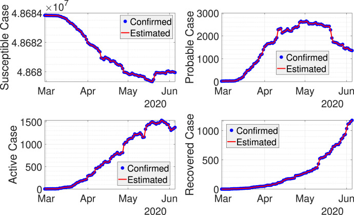
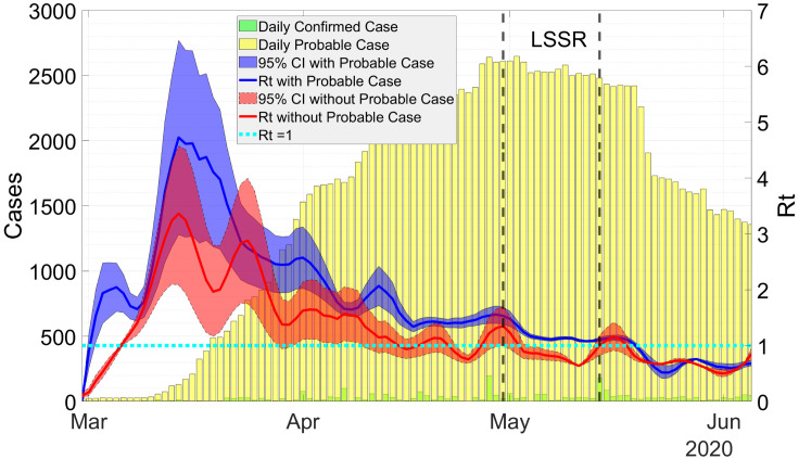
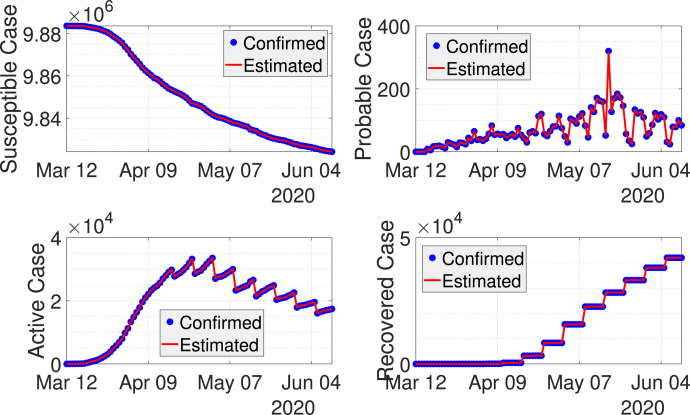
Fig. 3 shows results from dynamic data fitting using EKF for West Java province in Indonesia. As can be seen from this figure, the discrete-time stochastic augmented SPIR model together with the EKF are able to model the transmissions of COVID-19 accurately. The RRMSE${}_X$ using the chosen tuning parameters ${\mathit{Q}}_F$ and ${\mathit{R}}_F$ are given in Table 2, where the error is reasonably small. The estimated ${\mathcal{R}}_t$ can be seen from Fig. 4. Here, the value of ${\mathcal{R}}_t$ is higher when the probable cases are taken into account. The difference between the estimated ${\mathcal{R}}_t$ with and without probable cases becomes smaller once the rate of the probable cases decreases.

Fig. 3.

Real-time fitting of COVID-19 cases in West Java using EKF.

Table 2.

RRMSE between confirmed data and estimated data using EKF.

RRMSE${}_X$
Region	S	P	I	R	Total
West Java	4.2e−16	6.6e−04	1.3e−06	2.2e−06	6.7e−04
Michigan	5.7e−12	1.0e−04	2.5e−01	2.6e−03	2.6e−01

Fig. 4.

Estimation of ${\mathcal{R}}_t$ in West Java with and without probable cases. Estimation of ${\mathcal{R}}_t$ without probable case is obtained using the SIRD model [13].

On May 6, the government of West Java province enact a Large-Scale Social Restriction (LSSR). Control measures include: (i) dismissal of schools and workplaces, (ii) restrictions on religious activities, activities in public places, social and cultural activities, and (iii) restrictions on modes of transportation. The decision was taken based on the evaluation of ${\mathcal{R}}_t$, which according to WHO need to be done if ${\mathcal{R}}_t>1$. The restriction can be relaxed if ${\mathcal{R}}_t<1$ for fourteen consecutive days. Since the government officials estimated ${\mathcal{R}}_t$ without considering probable cases, the restriction was relaxed on May 20 when ${\mathcal{R}}_t<1$ for two weeks. Taking probable cases into account, our estimation shows that during the period of LSSR, the estimated value of ${\mathcal{R}}_t$ is still above 1. Thus, the LSSR need to be extended rather than relaxed. The effect of LSSR, where ${\mathcal{R}}_t<1$, can be seen after two weeks (May 24) since there are delays in infection confirmation.

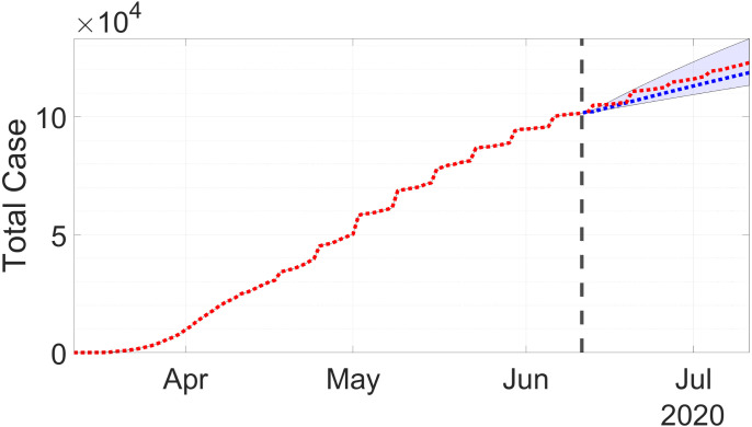
Using 95% confidence interval, forecasting result for the total case is presented in Fig. 5 by the dashed-blue line, whereas the confirmed data is presented by the dashed-red line. The forecast is done assuming the current measure is continued for the next 30 days. The figure shows the forecast is a bit higher than the confirmed data, but still inside the confidence interval. This could mean the government has tighten the measures, the number of testing was decreased, the transmission was successfully slowed down, or the combinations of those reasons.

Fig. 5.

Forecast for the number of total case in West Java. The dashed-red line is the actual or confirmed cases, while the dashed-blue line is the forecast. (For interpretation of the references to color in this figure legend, the reader is referred to the web version of this article.)

4.2. Michigan, USA

Fig. 6 shows data fitting results of COVID-19 cases in Michigan using EKF. It can be observed that the EKF estimates the confirmed cases accurately. As can be seen from Table 2, the RRSME is fairly small. Stay-at-home order was issued on March 24 by the government of Michigan. The order includes measures such as: (i) temporarily suspend in-person services that are not necessary for businesses and operations, (ii) asking residents to remain in their home, not to engage in outdoor activity, and practice social distancing. The order was lasting until May 15. The government started in-house testing for COVID-19 on March 16, with the capabilities to deliver same-day results. As a result, the number of daily probable cases is relatively low compare to the number of daily confirmed case, as can be seen from Fig. 7. Furthermore, as expected the estimation of ${\mathcal{R}}_t$ with and without probable cases is fairly similar. The stay-at-home order has been proven effective to reduce the transmission, indicated by ${\mathcal{R}}_t<1$ two weeks after being put into effect. However, we see that there is an increase in the number of daily cases once the order was repealed.

Fig. 6.

Real-time fitting of COVID-19 cases in Michigan using EKF.

Fig. 7.

Estimation of ${\mathcal{R}}_t$ in Michigan with and without probable cases.

Fig. 8 shows forecasting result for the number of total case in Michigan in the next 30 days. To show the quality of the forecast, we compare the forecast for the next 30 days using data until 11 June and the confirmed data from 12 June until 12 July. The forecast is slightly lower than the confirmed data but still inside the 95% confidence interval. This could mean the control measures were relaxed. In this case, the government should have to tighten the measures to control the transmissions.

Fig. 8.

Forecast for the number of total case in Michigan. The dashed-red line is the actual or confirmed cases, while the dashed-blue line is the forecast. (For interpretation of the references to color in this figure legend, the reader is referred to the web version of this article.)

5. Conclusion

A new compartmental epidemic model taking probable cases into account has been presented in this paper. The model, called the SPIR model, consists of four compartments: Susceptible (S), Probable (P), Active (I), and Recovered (R). The model is used to estimate the time-varying effective reproduction number ${\mathcal{R}}_t$ in West Java province in Indonesia and the state of Michigan in the USA. To this end, we apply an EKF to a discrete-time stochastic augmented SPIR model. Numerical simulations using data from West Java province show that when probable cases are taking into account, the value of ${\mathcal{R}}_t$ is significantly higher. However, if the number of probable cases is not significant, exemplified by the state of Michigan, the value of ${\mathcal{R}}_t$ is similar to regular methods. This results can be used to inform policy makers when deciding to loosen or tighten the measures. In general, our model and approach can be used in regions with limited testing capacity.

Declaration of Competing Interest

The authors declare that they have no known competing financial interests or personal relationships that could have appeared to influence the work reported in this paper.

References

- 1.Giordano G., Blanchini F., Bruno R., Colaneri P., Filippo A.D., Matteo A.D., et al. Modelling the COVID-19 epidemic and implementation of population-wide interventions in Italy. Nat Med. 2020;26:855–860. doi: 10.1038/s41591-020-0883-7. [DOI] [PMC free article] [PubMed] [Google Scholar]
- 2.Singhal A., Singh P., Lall B., Joshi S. Modeling and prediction of COVID-19 pandemic using Gaussian mixture model. Chaos Solitons Fractals. 2020;138:1–8. doi: 10.1016/j.chaos.2020.110023. [DOI] [PMC free article] [PubMed] [Google Scholar]
- 3.Hasan A., Susanto H., Kasim M., Nuraini N., Lestari B., Triany D., et al. Superspreading in early transmissions of COVID-19 in Indonesia. Sci Rep. 2020;10:1–4. doi: 10.1038/s41598-020-79352-5. [DOI] [PMC free article] [PubMed] [Google Scholar]
- 4.Bettencourt L., Ribeiro R. Real time Bayesian estimation of the epidemic potential of emerging infectious diseases. PLoS ONE. 2008;3:1–9. doi: 10.1371/journal.pone.0002185. [DOI] [PMC free article] [PubMed] [Google Scholar]
- 5.Cori A., Ferguson N., Fraser C., Cauchemez S. A new framework and software to estimate time-varying reproduction numbers during epidemics. Am J Epidemiol. 2013;178:1505–1512. doi: 10.1093/aje/kwt133. [DOI] [PMC free article] [PubMed] [Google Scholar]
- 6.Center for Disease Control and Prevention, Coronavirus Disease 2019 (COVID-19) 2020 Interim Case Definition, https://wwwn.cdc.gov/nndss/conditions/coronavirus-disease-2019-covid-19/case-definition/2020/.
- 7.Bartle R., Sherbert D. 4th ed. Wiley; 2011. Introduction to real analysis. [Google Scholar]
- 8.Lin W. Global existence theory and chaos control of fractional differential equations. J Math Anal Appl. 2007;332:709–726. doi: 10.1016/j.jmaa.2006.10.040. [DOI] [Google Scholar]
- 9.van den Driessche P., Watmough J. Reproduction numbers and sub-threshold endemic equilibria for compartmental models of disease transmission. Math Biosci. 2002;180:29–48. doi: 10.1016/S0025-5564(02)00108-6. [DOI] [PubMed] [Google Scholar]
- 10.Diekmann O., Heesterbeek J., Metz J. On the definition and the computation of the basic reproduction ratio in models for infectious diseases in heterogeneous populations. J Math Biol. 1990;28:365–382. doi: 10.1007/BF00178324. [DOI] [PubMed] [Google Scholar]
- 11.Brauer F., Castillo-Chavez C., Feng Z. 1st ed. Springer-Verlag; 2019. Mathematical models in epidemiology. [Google Scholar]
- 12.Simon D. 1st ed. Wiley-Interscience; 2006. Optimal state estimation: Kalman, H infinity, and nonlinear approaches. [Google Scholar]
- 13.Hasan A., Susanto H., Tjahjono V., Kusdiantara R., Putri E., Hadisoemarto P., et al. 2020. A new estimation method for COVID-19 time-varying reproduction number using active cases. MedRxiv (preprint) [DOI] [PMC free article] [PubMed] [Google Scholar]