Optimal control approach of a mathematical modeling with multiple delays of the negative impact of delays in applying preventive precautions against the spread of the COVID-19 pandemic with a case study of Brazil and cost-effectiveness

Highlights

• •We propose to study an optimal control approach with delay in state and control variables.
• •Numerical simulation of different strategies.
• •The cost of effectivness.

Abstract

As of June 02, 2020. The number of people infected with COVID-19 virus in Brazil was about 529,405, the number of death is 30046, the number of recovered is 211080, and the number is subject to increase. This is due to the delay by a number of countries in general, and Brazil in particular, in taking preventive and proactive measures to limit the spread of the COVID-19 pandemic. So, we propose to study an optimal control approach with delay in state and control variables in our mathematical model proposed by kouidere et al. which describes the dynamics of the transmission of the COVID-19. That the time with delay represent the delay to applying preventive precautions measures. Pontryagin’s maximum principle is used to characterize the optimal controls and the optimality system is solved by an iterative method. Finally, some numerical simulations are performed to verify the theoretical analysis using MATLAB.

1. Introduction

On December 31, 2019, the Chinese authorities announced a dangerous virus outbreak in the Chinese city of Wuhan. The virus was temporarily called the novel Coronavirus nCoV-19, then the International Virus Classification Committee named it (SARS-CoV-2) [19], [20]. This virus belongs to Corona viruses COVID-19 that infect the human respiratory system from seasonal colds. The danger of the novel Coronavirus 2019 lies in the fact that the infected person does not show symptoms of the disease in the incubation period, which ranges from two days to 14 days. The person then shows mild symptoms such as sneezing, a slight rise in temperature, then severe fatigue, a dangerous rise in temperature, difficulty breathing, and failure to breathe that leads to death, especially if the person suffers from a chronic disease such as diabetes, cancer, or HIV disease.

According to the World Health Organization [1], [2], [3]. The novel Coronavirus COVID-19 belongs to the strains of Coronaviruses, which are transmitted from animals to humans and between humans. The most prominent of these is the SARS virus [21], which also appeared for the first time in China and infected about 8098 people and caused the death of 774 people. The source of this virus was bats. Another virus of this strain is the Middle East Syndrome virus (MERS) [4], [5], [6], [7], which infected about 2498 people and resulted in the death of 858 people. The source of this virus was camels.

Compared to the rest of the Coronaviruses, COVID-19 virus is considered the most dangerous and the fastest in spread. Up to June 02, 2020, this virus caused about 6,400,055 infected cases, 378,069 deaths and 2,930,682 recovered cases. Following this huge spread around the world [13], [14], [24]. The WHO declared a state of emergency.

Globally, the number of infected people. In USA, about the infected individuals reached 1,859,772 and the deaths reached 106929. In Brazil, 529,405 people were infected and 30,046 died. In Russia, about 423,741 people were infected and 5037 died. According to the last stats declared on June 02, 2020. The epidemic has moved from China to Europe and to USA and now to South America, which has become the main epidemic area according to the World Health Organization.

On February 26, 2020, Brazilian authorities announced the first case of COVID-19, the first case recorded in South America, of a Brazilian national from Italy. The spread of the COVID-19 virus was initially stable. Then in recent weeks, where the spread of the virus has experienced tremendous acceleration, reaching in June 02, 2020, 3 months after the registration of the first case, approximately 529,405 infected, 30,046 deaths. Brazil has become the second country in the world in terms of infected, after the United States of America.

Where he recorded in State of S ao Paulo about 109,698 infected, followed by State of Rio de Janeiro about 53,388 infected, and in State of Ceará about 48,489 infected, and in State of Amazonas about 41,378 infected.

A large number of mathematical models have been developed to simulate, analyse and understand the Corona virus. In a related research work, Tian-Mu Chen et al. [8] proposed a mathematical model for simulating the phase-based transmissibility of a novel Coronavirus, and Zhi-Qiang Xia et al. [9] Early dynamics of transmission and control of COVID-19: a mathematical modeling study. Sunhwa Choi and Moran Ki proposed [8] Estimating the reproductive number and the outbreak size of Novel Coronavirus disease (COVID-19) using mathematical model in the Republic of Korea [22] Also, many researches have focused on this topic and other related topics [16], [17], [25], [26], [27], [28], [33], [40] . They have found the basic reproduction number $R_0$ and discussed the stability analysis of their model using the basic reproduction number. They found that the model is locally asymptotically stable at disease free equilibrium $E_0$ when $R_0<1$ and when $R_0>1,$ endemic equilibrium exists and becomes stable. In their research, equilibrium points are also globally asymptotically stable under certain conditions. Besides these, many mathematical models were formulated to investigate the dynamics of infectious diseases with control (For example: [30], [31], [32]).

But they did not take into account delay in applying precautionary and preventive measures which may cause a delay in response to the potential threats.

Delay in applying precautionary and preventive measures, such as:

• •The delay in schools closure in the affected countries.
• •The delay in closing airports and ports in a timely manner.
• •The delay in suspending air, land and navigation travels from and to the affected countries.
• •The delay in applying precautionary, preventive and strict measures when receiving travelers.
• •The delay in diagnosis of the infected cases, given that symptoms do not appear in the disease’s incubation period.
• •The tolerance of others in the passage of passengers through airports in some countries.
• •The delay in diagnosis of infected cases, especially as symptoms do not appear in the disease’s incubation period.
• •The delay in imposing quarantine among patients increases the spread of the disease.

Perhaps the delay in applying the aforementioned precautionary measures was the main reason that Western Europe turned into the main focus of the global pandemic. This led to panic as the number of the infected individuals and deaths keep rising. Thousands of infected cases and hundreds of deaths are recorded daily in Italy, Spain, Germany, the United States of America and France. In Italy, on Saturday, 21 March 2020, a record number of deaths reached nearly 800 deaths, and more than 6000 infected. The pandemic focus shifted from China to Western Europe and that led to the ease of transmission and spread of the disease in the neighboring countries and the countries of North Africa.

In addition, most of the previous research has focused on continuous modeling. In this research, the statistical data are collected at the time (day, week, month, and year). Treatment and vaccination of some patients are also given at the same time. Consequently, it is more direct, more practical, and more precise to describe a phenomenon using continuous temporal modeling. Thus, differential equations appear like a more natural way of describing epidemiological models. In addition, numerical solutions are used for the discretionary differential equations, which encourages us to use the differential equations directly. and therefore can be easily implemented by mathematicians.

To make the modeling of this phenomenon more realistic, we consider an optimal control problem governed by a system of differential equations with time to delay. We study an optimal control problem with time to delay in the state and control variable in a mathematical model $S{I}_{W}ICHR$ of kouidere et al. [25] and a time delay representing delay in applying preventive precaution and measures.

The paper is organized as follows: In Section 2, we represent our mathematical model $S{I}_{W}ICHR$, analysis of a mathematical modeling of transmission of novel coronavirus “COVID-19”. In Section 3, a mathematical modeling with optimal control startegy of transmission of novel coronavirus “COVID-19”. In Section 4, we present a optimal control problem with multiple delays in our proposed model where we give some results concerning the existence of the optimal control and we caracterize the optimal controls using the Pontryagin’s maximum principle. Numerical simulations through MATLAB are given in Section 5. Finally we conclude the paper in Section 6.

2. Mathematical model

We consider a mathematical model $S{I}_{W}ICHR$ of kouidere et al., that describes the of transmission of novel coronavirus “COVID-19”. We divide the population denoted by $N$ into six compartments: susceptible population Brazil $S,$ the infected without symptoms $I_W,$ the infected with symptoms $I,$ the infected with complications $C,$ the number of people who have been quarantined in hospitals $H$ and recovered $R.$

Hence, we present the COVID-2019 mathematical model is governed by the following system of differential equation:

$$\{\begin{array}{c}{\displaystyle \frac{dS\left(t\right)}{dt}}=\Lambda -\mu S\left(t\right)-{\beta }_1{\displaystyle \frac{S\left(t\right)I_W\left(t\right)}{N}}-{\beta }_2{\displaystyle \frac{S\left(t\right)I\left(t\right)}{N}}\hfill \\ \\ {\displaystyle \frac{d{I}_W\left(t\right)}{dt}}={\beta }_1{\displaystyle \frac{S\left(t\right)I_W\left(t\right)}{N}}+{\beta }_2{\displaystyle \frac{S\left(t\right)I\left(t\right)}{N}}-(\mu +{\alpha }_1+{\alpha }_2)I_W\left(t\right)\hfill \\ \\ {\displaystyle \frac{dI\left(t\right)}{dt}}={\alpha }_1{I}_W\left(t\right)-({\alpha }_3+{\theta }_1+\mu )I\left(t\right)\hfill \\ \\ {\displaystyle \frac{dC\left(t\right)}{dt}}={\alpha }_2{I}_W\left(t\right)+{\alpha }_{3}I\left(t\right)-({\theta }_2+\mu +{\delta }_1)C\left(t\right)\hfill \\ \\ {\displaystyle \frac{dH\left(t\right)}{dt}}={\theta }_{1}I\left(t\right)+{\theta }_{2}C\left(t\right)-(\mu +\sigma +{\delta }_2)H\left(t\right)\hfill \\ \\ {\displaystyle \frac{dR\left(t\right)}{dt}}=\sigma H\left(t\right)-\mu R\left(t\right)\hfill \end{array}$$ (1)

where $S\left(0\right)\ge 0,$ $I_W\left(0\right)\ge 0,$ $I\left(0\right)\ge 0,$ $C\left(0\right)\ge 0,$ $H\left(0\right)\ge 0$ and $R\left(0\right)\ge 0$ are the initial state.

With

- $\Lambda$: Denote the incidence of susceptible in Brazil.

- $\mu$: natural mortality

- ${\beta }_1$: The rate of people who were infected with the virus by contact with the infected patients without symptoms

- ${\beta }_2$: The rate of people who were infected with the virus by communicating with the infected patients with symptoms

- ${\alpha }_1$: The rate of people become normaly infected with symptoms

- ${\alpha }_2$: The rate of people have developed a rapid and dangerous development of the disease due to immunodeficiency, old age or children.

- ${\alpha }_3$: The rate of people have severe complications such as pulmonary failure.

- ${\theta }_1$: The rate of people with symptoms of mild virus who have been quarantined.

- ${\theta }_2$: The rate of people with serious complications who have been quarantined.

- $\sigma$: The rate of people who recovered from the virus.

- ${\delta }_1$: Mortality rate due to complications.

- ${\delta }_2:$ The rate of people who died under quarantine in hospitals.

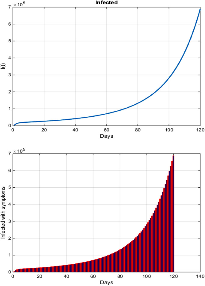
Fig. 1 shows that, if Brazil does not apply preventive precautions to reduce the spread of the COVID-19 pandemic, the number of COVID-19 infected cases is likely to reach millions.

Fig. 1.

Accumulated cases of COVID-19 in Brazil after 4 months.

2.1. Model basic properties

2.1.1. Positivity of solutions

Theorem 1

If $S\left(0\right)\ge 0,$ $I_W\left(0\right)\ge 0,$ $I\left(0\right)\ge 0,$ $C\left(0\right)\ge 0,$ $H\left(0\right)\ge 0$ and $R\left(0\right)\ge 0,$ the solutions $S\left(t\right),$ $I_W\left(t\right),I\left(t\right),C\left(t\right),H\left(t\right)$ and $R\left(t\right)$ of system (15) are positive for all $t\ge 0$ .

Proof

It follows from the first equation of system (15) that

$$\begin{array}{ccc}\hfill \frac{dS\left(t\right)}{dt}& =& {\Lambda }_1-\mu S\left(t\right)-{\beta }_1\frac{S\left(t\right)I_W\left(t\right)}{N}-{\beta }_2\frac{S\left(t\right)I\left(t\right)}{N}\hfill \\ & \ge & -\mu S\left(t\right)-{\beta }_1\frac{S\left(t\right)I_W\left(t\right)}{N}-{\beta }_2\frac{S\left(t\right)I\left(t\right)}{N}\hfill \end{array}$$

$$\frac{dS\left(t\right)}{dt}+(\mu +{\beta }_1\frac{I_W\left(t\right)}{N}+{\beta }_2\frac{I\left(t\right)}{N})S\left(t\right)\ge 0$$

where $F\left(t\right)=\mu +{\beta }_1\frac{I_W\left(t\right)}{N}+{\beta }_2\frac{I\left(t\right)}{N}.$ The both sides in last inequality are multiplied by $\exp \left(\underset{0}{\overset{t}{\int }}F\left(s\right)ds\right).$

We obtain

$$\exp \left(\underset{0}{\overset{t}{\int }}F\left(s\right)ds\right).\frac{dS\left(t\right)}{dt}+F\left(t\right)\exp \left(\underset{0}{\overset{t}{\int }}F\left(s\right)ds\right).S\left(t\right)\ge 0$$

then $\frac{d}{dt}\left(S\left(t\right)\exp \right(\underset{0}{\overset{t}{\int }}F\left(s\right)ds\left)\right)\ge 0$

Integrating this inequality from 0 to $t$ gives:

$$\underset{0}{\overset{t}{\int }}\frac{d}{ds}\left(S\left(s\right)\exp \left(\underset{0}{\overset{t}{\int }}(\mu +{\beta }_1\frac{I_W\left(s\right)}{N}+{\beta }_2\frac{I\left(s\right)}{N})ds\right)\right)ds\ge 0$$

then

$$S\left(t\right)\ge S\left(0\right)\exp (-\underset{0}{\overset{t}{\int }}(\mu +{\beta }_1\frac{I_W\left(s\right)}{N}+{\beta }_2\frac{I\left(s\right)}{N})ds)$$

$⟹S\left(t\right)\ge 0$.

Similarly, we prove that $I_W\left(t\right)\ge 0I\left(t\right)\ge 0,C\left(t\right)\ge 0,H\left(t\right)\ge 0$ and $R\left(t\right)>0.$  □

2.1.2. Boudedness of the solutions

Theorem 2

The set $\Omega =\{(S,I_W,I,C,H,R)\in {\mathbb{R}}_{+}^6/0\le S+I_W+I+C$ $+H+R\le \frac{\Lambda }{\mu }\}$ positively invariant under system (15) with initial conditions $S\left(0\right)\ge 0,$ $I_W\left(0\right)\ge 0,$ $I\left(0\right)\ge 0,$ $C\left(0\right)\ge 0,$ $H\left(0\right)\ge 0$ and $R\left(0\right)\ge 0$ .

Proof

Also, one assumes that:

$$\begin{array}{ccc}\hfill \frac{dN}{dt}& =& \Lambda -\mu N-{\delta }_{1}C\le \Lambda -\mu N\hfill \\ & ⟹& N\left(t\right)\le \frac{\Lambda }{\mu }+N\left(0\right)e^{-\mu t}\hfill \end{array}$$

If we take limit $t\to \infty$we have$0\le N\left(t\right)\le \frac{\Lambda }{\mu }$.

It implies that the region $\Omega$ is a postivily invariant set for the system (15). □

2.1.3. Exictence of solutions

Theorem 3

The system (15) that satisfies a given initial condition

$(S\left(0\right),I_W\left(0\right),I\left(0\right).C\left(0\right),H\left(0\right),R\left(0\right))$ has a unique solution.

Proof

Let $X=\left(\begin{array}{c}S\left(t\right)\\ I_W\left(t\right)\\ I\left(t\right)\\ C\left(t\right)\\ H\left(t\right)\\ R\left(t\right)\end{array}\right)$ and $\phi \left(X\right)=\left(\begin{array}{c}\frac{dS\left(t\right)}{dt}\\ \\ \frac{d{I}_W\left(t\right)}{dt}\\ \\ \frac{dI\left(t\right)}{dt}\\ \\ \frac{dC\left(t\right)}{dt}\\ \\ \frac{dH\left(t\right)}{dt}\\ \\ \frac{dR\left(t\right)}{dt}\end{array}\right)$ so the system (15) can be rewritten in the following form:

$$\phi \left(X\right)=AX+B\left(X\right)$$ (2)

where

$$A=\left(\begin{array}{cccccc}-\mu & 0& -0& 0& 0& 0\\ 0& -(\mu +{\alpha }_1+{\alpha }_2)& 0& 0& 0& 0\\ 0& {\alpha }_1& -({\alpha }_3+{\theta }_1+\mu )& 0& 0& 0\\ 0& {\alpha }_2& {\alpha }_3& -({\theta }_2+\mu +{\delta }_1)& 0& 0\\ 0& 0& {\theta }_1& {\theta }_2& -(\mu +\sigma +{\delta }_2)& 0\\ 0& 0& 0& 0& \sigma & -\mu \end{array}\right)$$

and

$$B\left(X\right)=\left(\begin{array}{c}\Lambda -{\beta }_1\frac{S\left(t\right)I_W\left(t\right)}{N}-{\beta }_2\frac{S\left(t\right)I\left(t\right)}{N}\\ \\ {\beta }_1\frac{S\left(t\right)I_W\left(t\right)}{N}+{\beta }_2\frac{S\left(t\right)I\left(t\right)}{N}\\ 0\\ 0\\ 0\\ 0\end{array}\right)$$

The second term on the right-hand side of (8) satisfies

$|B\left(X_1\right)-B\left(X_2\right)|=2|{\beta }_1\frac{S_1\left(t\right)I_{W.1}\left(t\right)}{N}+{\beta }_2\frac{S_1\left(t\right)I_1\left(t\right)}{N}-{\beta }_1\frac{S_2\left(t\right)I_{W.2}\left(t\right)}{N}$ $-{\beta }_2\frac{S_2\left(t\right)I_2\left(t\right)}{N}|$

$=2\left|\begin{array}{c}{\beta }_1\frac{S_1\left(t\right)I_{W.1}\left(t\right)}{N}+{\beta }_1\frac{S_1\left(t\right)I_{W.2}\left(t\right)}{N}-{\beta }_1\frac{S_1\left(t\right)I_{W.2}\left(t\right)}{N}-{\beta }_2\frac{S_1\left(t\right)I_1\left(t\right)}{N}\\ +{\beta }_2\frac{S_1\left(t\right)I_2\left(t\right)}{N}-{\beta }_2\frac{S_1\left(t\right)I_2\left(t\right)}{N}-{\beta }_1\frac{S_2\left(t\right)I_{W.2}\left(t\right)}{N}+{\beta }_2\frac{S_2\left(t\right)I_2\left(t\right)}{N}\end{array}\right|$

$\le 2\left(\begin{array}{c}\left|\frac{{\beta }_1{S}_1\left(t\right)}{N}\right||I_{W.1}\left(t\right)-I_{W.2}\left(t\right)|+\left|\frac{{\beta }_1{I}_{W.2}\left(t\right)}{N}\right||S_1\left(t\right)-S_2\left(t\right)|\\ +\left|\frac{{\beta }_2{S}_1\left(t\right)}{N}\right||I_1\left(t\right)-I_2\left(t\right)|+\left|\frac{{\beta }_2{I}_2\left(t\right)}{N}\right||S_1\left(t\right)-S_2\left(t\right)|\end{array}\right)$

$\le 2\frac{Z}{\mu }\left(\begin{array}{c}\left|\frac{{\beta }_1}{N}\right||I_{W.1}\left(t\right)-I_{W.2}\left(t\right)|+\left|\frac{{\beta }_1}{N}\right||S_1\left(t\right)-S_2\left(t\right)|\\ +\left|\frac{{\beta }_2}{N}\right||I_1\left(t\right)-I_2\left(t\right)|+\left|\frac{{\beta }_2}{N}\right||S_1\left(t\right)-S_2\left(t\right)|\end{array}\right)$

$\le M\left(|X_1\left(t\right)-X_2\left(t\right)|\right)$

Where $M=2\frac{Z}{\mu }(\left|\frac{{\beta }_1}{N}\right|+\left|\frac{{\beta }_2}{N}\right|;\left|\frac{{\beta }_1}{N}\right|+\left|\frac{{\beta }_2}{N}\right|)$ then

$$\parallel \phi \left(X_1\right)-\phi \left(X_2\right)\parallel \le V.\parallel X_1-X_2\parallel$$

where $V=\max (M,\parallel A\parallel )<\infty$.

Thus, it follows that the function $\phi$ is uniformly Lipschitz continuous, and the restriction on $S\left(t\right)\ge 0,$ $I_W\left(t\right)\ge 0$ $I\left(t\right)\ge 0,$ $C\left(t\right)\ge 0,$ $H\left(t\right)\ge 0$ and $R\left(t\right)\ge 0,$ we see that a solution of the system exists [18]. □

3. Stability analysis and sensitivity of the model parameters

In this section, we will study the stability behavior of system (1) at an Disease Free Equilibrium point is denoted by $E^0$ and an Endemic Equilibrium point is denoted by $E^{*}$. The first three equations in system (1) are independent of the variables $C,H$ and $R$. Hence, the dynamics of equation system (1) is equivalent to the dynamics of the equation system:

$$\{\begin{array}{c}{\displaystyle \frac{dS\left(t\right)}{dt}}=\Lambda -\mu S\left(t\right)-{\beta }_1{\displaystyle \frac{S\left(t\right)Iw\left(t\right)}{N}}-{\beta }_2{\displaystyle \frac{S\left(t\right)I\left(t\right)}{N}}\hfill \\ \\ {\displaystyle \frac{dIw(t}{dt}}={\beta }_1{\displaystyle \frac{S\left(t\right)Iw\left(t\right)}{N}}+{\beta }_2{\displaystyle \frac{S\left(t\right)I\left(t\right)}{N}}-(\mu +{\alpha }_1+{\alpha }_2)Iw\left(t\right)\hfill \\ \\ {\displaystyle \frac{dI\left(t\right)}{dt}}={\alpha }_1{I}_W\left(t\right)-({\alpha }_3+{\theta }_1+\mu )I\left(t\right)\hfill \end{array}$$ (3)

3.1. Equilibrium point

3.1.1. The disease free equilibrium

To find the disease free equilibrium point, we equated the right hand side of model (1) to zero, evaluating it at $I_w=I$=0 and solving for the noninfected and noncarrier state variables. Therefore, the disease free equilibrium point $E^0=(\frac{\Lambda }{\mu },0,0).$

3.1.2. The endemic equilibrium

The endemic equilibrium point $E^{*}=(S^{*},I_w^{*},I^{*})$ it occurs when the disease persists in the community. To obtain it, we equate all the model Eq. (1) to zero. then we obtain

$S^{*}=\frac{\Lambda }{\mu R_0}$

$I_w^{*}=\frac{\Lambda (R_0-1)}{(\mu +{\alpha }_1+{\alpha }_2)R_0}$

$I^{*}=\frac{{\alpha }_1\Lambda (R_0-1)}{({\alpha }_3+{\theta }_1+\mu )(\mu +{\alpha }_1+{\alpha }_2)R_0}$ where $R_0$ is the basic reproduction number given by:

$R_0=\frac{{\beta }_1({\alpha }_3+{\theta }_1+\mu )+{\beta }_2{\alpha }_1}{({\alpha }_3+{\theta }_1+\mu )(\mu +{\alpha }_1+{\alpha }_2)}$

3.2. The basic reproductive number

In our work, the basic reproduction number $R_0$ is defined as the average number of secondary infections produced by an infected individual in a completely susceptible population. To obtain the basic reproduction number, we used the next-generation matrix method formulated in Bentout et al. [34], Bani-Yaghoub et al. [35], Driessche and Watmough [36].

Through the model equations system (2), then by the principle of next generation matrix, we obtained:

$$\mathrm{f}=\left(\begin{array}{c}-{\beta }_1{\displaystyle \frac{S\left(t\right)Iw\left(t\right)}{N}}-{\beta }_2{\displaystyle \frac{S\left(t\right)I\left(t\right)}{N}}\\ \\ {\beta }_1{\displaystyle \frac{S\left(t\right)Iw\left(t\right)}{N}}+{\beta }_2{\displaystyle \frac{S\left(t\right)I\left(t\right)}{N}}\\ 0\end{array}\right)$$

$$\mathrm{v}=\left(\begin{array}{c}-\Lambda +\mu S\left(t\right)\\ (\mu +{\alpha }_1+{\alpha }_2)Iw\left(t\right)\\ ({\alpha }_3+{\theta }_1+\mu )I\left(t\right)-{\alpha }_{1}Iw\left(t\right)\end{array}\right)$$

where

$$\mathrm{F}=\left(\begin{array}{ccc}0& -{\beta }_1& -{\beta }_2\\ 0& {\beta }_1& {\beta }_2\\ 0& 0& 0\end{array}\right)$$

$$\mathrm{V}=\left(\begin{array}{ccc}\mu & 0& 0\\ 0& (\mu +{\alpha }_1+{\alpha }_2)& 0\\ 0& -{\alpha }_1& ({\alpha }_3+{\theta }_1+\mu )\end{array}\right)$$

The inverse of V is given by

$${\mathrm{V}}^{-1}=\left(\begin{array}{ccc}{\displaystyle \frac{1}{\mu }}& 0& 0\\ 0& {\displaystyle \frac{1}{(\mu +{\alpha }_1+{\alpha }_2)}}& 0\\ 0& {\displaystyle \frac{{\alpha }_1}{(\mu +{\alpha }_1+{\alpha }_2)({\alpha }_3+{\theta }_1+\mu )}}& {\displaystyle \frac{1}{({\alpha }_3+{\theta }_1+\mu )}}\end{array}\right)$$

then

$$\begin{array}{ccc}& & {\text{FV}}^{-1}\hfill \\ & & =\left(\begin{array}{ccc}0& -({\displaystyle \frac{{\beta }_1}{\mu +{\alpha }_1+{\alpha }_2}}+{\displaystyle \frac{{\beta }_2{\alpha }_1}{(\mu +{\alpha }_1+{\alpha }_2)({\alpha }_3+{\theta }_1+\mu )}})& {\displaystyle \frac{-{\beta }_2}{{\alpha }_3+{\theta }_1+\mu }}\\ 0& ({\displaystyle \frac{{\beta }_1}{\mu +{\alpha }_1+{\alpha }_2}}+{\displaystyle \frac{{\beta }_2{\alpha }_1}{(\mu +{\alpha }_1+{\alpha }_2)({\alpha }_3+{\theta }_1+\mu )}})& {\displaystyle \frac{{\beta }_2}{{\alpha }_3+{\theta }_1+\mu }}\\ 0& 0& 0\end{array}\right)\hfill \end{array}$$

Finally, we have

$R_0=\rho \left(F{V}^{-1}\right)={\displaystyle \frac{{\beta }_1({\alpha }_3+{\theta }_1+\mu )+{\beta }_2{\alpha }_1}{(\mu +{\alpha }_1+{\alpha }_2)({\alpha }_3+{\theta }_1+\mu )}}$

3.3. Local stability of disease free equilibrium

Theorem 4

The disease free equilibrium point $E^0$ is locally asymptotically stable if $R_0<1$ and unstable if $R_0>1$ .

Proof

The Jacobian matrix of system (3) at the disease free equilibrium point $E^0$ as follows:

$$\mathrm{J}\left({\mathrm{E}}^0\right)=\left(\begin{array}{ccc}-\mu & -{\beta }_1& -{\beta }_2\\ 0& -(\mu +{\alpha }_1+{\alpha }_2-{\beta }_1)& {\beta }_2\\ 0& {\alpha }_1& -({\alpha }_3+{\theta }_1+\mu )\end{array}\right)$$

From the jacobian matrix $J\left(E^0\right)$ we obtained a characteristic polynomial:

$p\left(\lambda \right)=(\mu +\lambda )({\lambda }^2+a\lambda +b)=0$ with

$a={\displaystyle \frac{{({\alpha }_3+{\theta }_1+\mu )}^2+{\beta }_2{\alpha }_1}{{\alpha }_3+{\theta }_1+\mu }}+(\mu +{\alpha }_1+{\alpha }_2)(1-R_0)$

$b=(\mu +{\alpha }_1+{\alpha }_2)({\alpha }_3+{\theta }_1+\mu )(1-R_0)$ we see that the characteristic equation $p\left(\lambda \right)$ of $J\left(E^0\right)$ has an eigenvalue ${\lambda }_1=-\mu$ is negative. So, in order to determine the stability of the $E^0,$ we discuss the roots of the following equation ${\lambda }^2+a\lambda +b=0$.

By Routh-Hurwitz criterion, system (2) is locally stable if $a>0$ and $b>0$.

Obviously we see that a and b to be positive, $(1-R_0)$ must be positive, which leads to $R_0<1$.

So $E^0$ is stable if $R_0<1$ and unstable if $R_0>1$. □

3.4. Numerical simulation

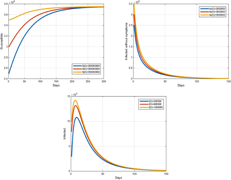
In this section, we present some numerical solutions of system (1) for different values of the parameters. The resolution of system (1) was created using the Gauss-Seidel-like implicit finite-difference method developed by LaSalle [37], presented in Gumel et al. [38] and denoted the GSS1 method. We use the different initial values for each variable of state, and we use the following parameters: $\Lambda =8,5.{10}^5$ $\mu =0.02,$ ${\alpha }_1=0.8,$ ${\alpha }_2=0.2,{\alpha }_3=0.2,$ ${\beta }_1=0.12,$ ${\beta }_2=0.1,$ ${\theta }_1=0.1,$ we have the Disease free Equilibrium point $E^0=(375.{10}^6,0,0,0,0).$ and $R_0=0.6059<1$. In this case, we obtained the following remarks: Over time, we notice that the number of susceptible people is close to $375.{10}^6$. We also note that the number of the people infected without symptoms and the number of the people infected with symptoms, are close to zero (see Fig. 2 ).

Fig. 2.

COVID-19 model with a disease-free equilibrium.

We start by a graphic representation of the COVID-19 disease-free equilibrium $E_0$ and we use the same parameters and different initial values in table1. $R_0=0.6059<1$ $R_0<1$. From these figures, using the different values of initial variables $S_0,I_{W0}$ and $I_0$ we obtained the following remarks: The number of potential individuals increases and approaches the number $S_0=1536$ (see Fig. 2): Also, the number of the asymptomatic infected cases or cases with mild symptoms decreases and converges to zero (see Fig. 2). The number of the infected people with symptoms and carriers of the virus increases at first, after that it decreases and approaches zero (see Fig. 2). Therefore, the solution curves to the equilibrium $E^0$ = $(S^0,0,0)$ when $R_0<1$. Hence, model (1) is stable.

According to theorem (3), the Disease free equilibrium point $E^0$ of system (1) is stable on $\Omega .$

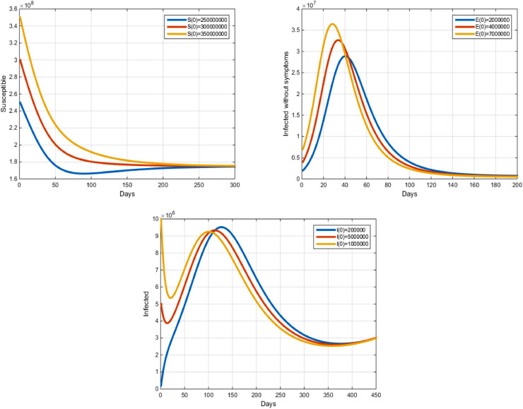
Also, for the different initial values for each variable of state, and the following parameters: $\Lambda =8,5.{10}^5,$ $\mu =0.02,$ ${\alpha }_1=0.8,$ ${\alpha }_2=0.2,{\alpha }_3=0.2,$ ${\beta }_1=0.35,$ ${\beta }_2=0.3,$ ${\theta }_1=0.1,$ we have the Endemic Equilibrium point $E^{*}=(1.7.{10}^8,1.504.{10}^6,3.5.{10}^6)$ and $R_0=1.8734>1$. In this case, we obtained the following remarks: Over time, we notice that the number of susceptible people is close to $1,7.{10}^8$. We also note that the number of the people infected without symptoms is close to $1.504.{10}^6,$ and the number of the people infected with symptoms are close to $3.5.{10}^6$ (see Fig. 3 ).

Fig. 3.

COVID-19 model with an epidemic equilibrium.

Therefore the solution curves to the equilibruim point $E^{*}$ when $R_0>1$.

3.5. Sensitivity analysis of model parameters

we performed a sensitivity analysis, On the basic parameters. to help us to know the parameters that have a high impact on the breeding number of base $R_0$.

To achieve a sensitivity analysis of the model (1), we followed the technique described by Karrakchou et al. [39].

This technique develops a formula to obtain the sensitivity index of all the basic parameters, defined as ${▵}_x^{R_0}=\frac{x}{R_0}*\frac{ðR_0}{ðx},$ for $x$ represents all the basic parameters. The sensitivity index of $R_0$ with respect to the remaining parameters are computed as follows:

${▵}_{\mu }^{R_0}=\frac{\mu }{R_0}*\frac{ðR_0}{ð\mu }=-\mu [\frac{1}{(\mu +{\alpha }_1+{\alpha }_2)}+\frac{{\beta }_2{\alpha }_1}{({\alpha }_3+{\theta }_1+\mu )({\beta }_1({\alpha }_3+{\theta }_1+\mu )+{\beta }_2{\alpha }_1)}]$

${▵}_{{\alpha }_1}^{R_0}=\frac{{\alpha }_1}{R_0}*\frac{ðR_0}{ð{\alpha }_1}=\frac{{\alpha }_1[{\beta }_2(\mu +{\alpha }_2)-{\beta }_1{(\mu +{\alpha }_3+{\theta }_1)}^2]}{(\mu +{\alpha }_1+{\alpha }_2)({\alpha }_3+{\theta }_1+\mu )[{\beta }_1({\alpha }_3+{\theta }_1+\mu )+{\beta }_2{\alpha }_1]}$

${▵}_{{\alpha }_2}^{R_0}=\frac{{\alpha }_2}{R_0}*\frac{ðR_0}{ð{\alpha }_2}=\frac{-{\alpha }_2}{\mu +{\alpha }_1+{\alpha }_2}$

${▵}_{{\alpha }_3}^{R_0}=\frac{{\alpha }_3}{R_0}*\frac{ðR_0}{ð{\alpha }_3}=\frac{-{\alpha }_1{\beta }_2}{({\alpha }_3+{\theta }_1+\mu )[{\beta }_1({\alpha }_3+{\theta }_1+\mu )+{\beta }_2{\alpha }_1]}$

${▵}_{{\beta }_1}^{R_0}=\frac{{\beta }_1}{R_0}*\frac{ðR_0}{ð{\beta }_1}=\frac{{\beta }_1(\mu +{\alpha }_3+{\theta }_1)}{{\beta }_1(\mu +{\alpha }_3+{\theta }_1)+{\beta }_2{\alpha }_1}$

${▵}_{{\beta }_2}^{R_0}=\frac{{\beta }_2}{R_0}*\frac{ðR_0}{ð{\beta }_2}=\frac{{\beta }_2{\alpha }_1}{{\beta }_1({\alpha }_3+{\theta }_1+\mu )+{\beta }_2{\alpha }_1}$

${▵}_{{\theta }_1}^{R_0}=\frac{{\theta }_1}{R_0}*\frac{ðR_0}{ð{\theta }_1}=\frac{-{\theta }_1{\beta }_2{\alpha }_1}{(\mu +{\alpha }_3+{\theta }_1)[{\beta }_1(\mu +{\alpha }_3+{\theta }_1)+{\beta }_2{\alpha }_1]}$ are obtained and evaluated at (Table 1 ).

Table 1.

The sensitivity of indices.

Parameter symbol	Value	Sensitivity indexes
$\mu$	0.02	$-$0.0672
${\alpha }_1$	0.8	$-$0.3273
${\alpha }_2$	0.2	$-$0.2667
${\alpha }_3$	0.2	$-$0.4947
${\beta }_1$	0.35	0.7383
${\beta }_2$	0.3	0.2613
${\theta }_1$	0.1	$-$0.2473

Their sensitivity indices are in Table 1.

4. The optimal control problem

4.1. Problem statement

As of today June 02, 2020, there is no cure or vaccine for the disease. So, we suggest the following strategies: there are four controls $u\left(t\right),$ $v\left(t\right),$ $w\left(t\right)$ and $z\left(t\right)$ for $t\in [0,T],$ that represent consecutively the awareness program through sensitization and prevention, quarantine and health monitoring, diagnosis, monitoring and the last is treatment and psychological support with follow-up at time t. In order to have a realistic and logic model, we need to take in consideration that the movement of controlled individuals from the compartment of Infected without symptoms ($I_W$) to quarantined in hospitals ($H$), and transition by the contact between Infected without symptoms (Respectively Infected with symptoms) with susceptible to susceptible, and the transition of Infected with symptoms (Respectively Infected with complications) to quarantined in hospitals, and the transition of quarantined in hospitals to rocovered is subject to a delay. Thus, the time delay is introduced into the system as follows: at the moment,Thus, the delay is introduced into the system as follows: in time, only a percentage of individuals ($I_W,C,I,H$) that have been treated and controlled ${\tau }_i$ time unit ago, that is to say that at the time $k-{\tau }_i$ with $i\in \{1,2,3,4\},$ are removed to other compartments.

So, the mathematical system with time delay in state and control system of variables is given by the nonlinear retarded system of differential equations:

$$\{\begin{array}{c}{\displaystyle \frac{dS\left(t\right)}{dt}}=\Lambda -\mu S\left(t\right)-{\beta }_1{\displaystyle \frac{S\left(t\right)I_W\left(t\right)}{N}}-{\beta }_2{\displaystyle \frac{S\left(t\right)I\left(t\right)}{N}}+{\beta }_{1}u(t-{\tau }_1)\hfill \\ \\ {\displaystyle \frac{S(t-{\tau }_1)I_W(t-{\tau }_1)}{N}}+{\beta }_{2}u(t-{\tau }_1){\displaystyle \frac{S(t-{\tau }_1)I(t-{\tau }_1)}{N}}\hfill \\ \\ {\displaystyle \frac{d{I}_W\left(t\right)}{dt}}={\beta }_1(1-u\left(t\right)){\displaystyle \frac{S\left(t\right)I_W\left(t\right)}{N}}+{\beta }_2(1-u\left(t\right)){\displaystyle \frac{S\left(t\right)I\left(t\right)}{N}}\hfill \\ \\ -(\mu +{\alpha }_1+{\alpha }_2)I_W\left(t\right)-w\left(t\right)I_W\left(t\right)\hfill \\ \\ {\displaystyle \frac{dI\left(t\right)}{dt}}={\alpha }_1{I}_W\left(t\right)-({\alpha }_3+{\theta }_1+\mu )I\left(t\right)-v\left(t\right)I\left(t\right)\hfill \\ \\ {\displaystyle \frac{dC\left(t\right)}{dt}}={\alpha }_2{I}_W\left(t\right)+{\alpha }_{3}I\left(t\right)-({\theta }_2+\mu +{\delta }_1)C\left(t\right)-v\left(t\right)C\left(t\right)\hfill \\ \\ {\displaystyle \frac{dH\left(t\right)}{dt}}={\theta }_{1}I\left(t\right)+{\theta }_{2}C\left(t\right)-(\mu +\sigma +{\delta }_2)H\left(t\right)+w(t-{\tau }_3)I_W\hfill \\ \\ (t-{\tau }_3)+v(t-{\tau }_2)(I(t-{\tau }_2)+C(t-{\tau }_2))-z\left(t\right)H\left(t\right)\hfill \\ \\ {\displaystyle \frac{dR\left(t\right)}{dt}}=\sigma H\left(t\right)-\mu R\left(t\right)+z(t-{\tau }_4)H(t-{\tau }_4)\hfill \end{array}$$ (4)

In addition, for biological reasons, we assume, for $\phi$ $\in$ $[-\tau ,0],$ that $S_{\phi },$ $I_{W\phi },$ $I_{\phi },$ $C_{\phi },$ $H_{\phi }$ and $R_{\phi }$ are nonnegative continuous functions and $u_{\phi }=0,v_{\phi }=0,w_{\phi }=0$ and $z_{\phi }=0$.

4.2. Model basic properties

4.2.1. Boudedness of the solutions

Theorem 5

The set $\Omega =\{(S,I_W,I,C,H,R)\in {\mathbb{R}}_{+}^6/0\le S+I_W+I+C$ $+H+R\le \frac{\Lambda }{\mu }\}$ is positively invariant under system (4) with initial conditions, $S\left(0\right)\ge 0,$ $I_W\left(0\right)\ge 0,$ $I\left(0\right)\ge 0,$ $C\left(0\right)\ge 0,$ $H\left(0\right)\ge 0$ and $R\left(0\right)\ge 0$ .

Proof

By adding the equations of system (4) we obtain

$$\begin{array}{ccc}\hfill {\displaystyle \frac{dN}{dt}}& =& \Lambda -\mu N-{\delta }_{1}C\le \Lambda -\mu N\hfill \\ & ⟹& N\left(t\right)\le {\displaystyle \frac{\Lambda }{\mu }}+N\left(0\right)e^{-\mu t}\hfill \end{array}$$

If we take limit $t\to \infty$we have$0\le N\left(t\right)\le \frac{\Lambda }{\mu }$.

It implies that the region $\Omega$ is a postivily invariant set for the system (4). □

4.2.2. Existence of solutions

Theorem 6

The controlled system (4) that satisfies the given initial condition

$(S\left(0\right),I_W\left(0\right),I\left(0\right),C\left(0\right),H\left(0\right),R\left(0\right))$ has a unique solution.

Proof

Let $X=\left(\begin{array}{c}S\left(t\right)\\ I_W\left(t\right)\\ I\left(t\right)\\ C\left(t\right)\\ H\left(t\right)\\ R\left(t\right)\end{array}\right)$ and $\phi \left(X\right)=\left(\begin{array}{c}{\displaystyle \frac{dS\left(t\right)}{dt}}\\ {\displaystyle \frac{d{I}_W\left(t\right)}{dt}}\\ {\displaystyle \frac{dI\left(t\right)}{dt}}\\ {\displaystyle \frac{dC\left(t\right)}{dt}}\\ {\displaystyle \frac{dH\left(t\right)}{dt}}\\ {\displaystyle \frac{dR\left(t\right)}{dt}}\end{array}\right)$

So the system (4) can be rewritten in the following form:

$$\phi \left(X\right)=AX+B\left(X\right)+C\left(X_{\tau }\right)$$ (5)

where

$$A=\left(\begin{array}{cccccc}-\mu & 0& -0& 0& 0& 0\\ \\ 0& A_1& 0& 0& 0& 0\\ \\ 0& {\alpha }_1& A_2& 0& 0& 0\\ \\ 0& {\alpha }_2& {\alpha }_3& A_3& 0& 0\\ \\ 0& 0& {\theta }_1& {\theta }_2& A_4& 0\\ \\ 0& 0& 0& 0& \sigma & -\mu \end{array}\right)$$

where $A_1=-($ $\mu$ $+{\alpha }_1+{\alpha }_2+w\left(t\right)),$ $A_2=-({\alpha }_3+{\theta }_1+\mu +v\left(t\right)),A_3=$ $-({\theta }_2+\mu +{\delta }_1+v\left(t\right))$ and $A_4=-(\mu +\sigma +{\delta }_2+z\left(t\right))$ and

$$B\left(X\right)=\left(\begin{array}{c}\Lambda -{\beta }_1{\displaystyle \frac{S\left(t\right)I_W\left(t\right)}{N}}-{\beta }_2{\displaystyle \frac{S\left(t\right)I\left(t\right)}{N}}\\ {\beta }_1(1-u\left(t\right)){\displaystyle \frac{S\left(t\right)I_W\left(t\right)}{N}}+{\beta }_2(1-u\left(t\right)){\displaystyle \frac{S\left(t\right)I\left(t\right)}{N}}\\ 0\\ 0\\ 0\\ 0\end{array}\right)$$

and

$$\begin{array}{ccc}& & C\left(X_{\tau }\right)\hfill \\ & & =\left(\begin{array}{c}{\beta }_{1}u(t-{\tau }_1){\displaystyle \frac{S(t-{\tau }_1)I_W(t-{\tau }_1)}{N}}+{\beta }_{2}u(t-{\tau }_1){\displaystyle \frac{S(t-{\tau }_1)I(t-{\tau }_1)}{N}}\\ 0\\ 0\\ 0\\ w(t-{\tau }_3)I_W(t-{\tau }_3)+v(t-{\tau }_2)(I(t-{\tau }_2)+C(t-{\tau }_2))\\ z(t-{\tau }_4)H(t-{\tau }_4)\end{array}\right)\hfill \end{array}$$

The second term on the right-hand side of (5) satisfies

$$|B\left(X_1\right)-B\left(X_2\right)|\le M_1.\parallel X_1-X_2\parallel$$

and

$$|C\left(X_{1\tau }\right)-C\left(X_{2\tau }\right)|\le M_2.\parallel X_{1\tau }-X_{2\tau }\parallel$$

where $M_1$ and $M_2$ are some positive constants, independent of the state variables $S\left(t\right),$ $I_W\left(t\right),$ $I\left(t\right),$ $C\left(t\right),$ $H\left(t\right)$ and $R\left(t\right)$.

Then

$$\parallel \phi \left(X_1\right)-\phi \left(X_2\right)\parallel \le V.\parallel X_1-X_2\parallel$$

where $V=\max (M_1,M_1,\parallel A\parallel )<\infty$.

Thus, it follows that the function $\phi$ is uniformly Lipschitz continuous, From the definition of the controls $u\left(t\right),$ $v\left(t\right),$ $w\left(t\right)$ and $z\left(t\right)$ and the restriction on $S\left(t\right)\ge 0,$ $I_W\left(t\right)\ge 0$ $I\left(t\right)\ge 0,$ $C\left(t\right)\ge 0,$ $H\left(t\right)\ge 0$ and $R\left(t\right)\ge 0,$ we prove that a solution of the system exists [18]. □

4.3. The optimal control: existence and characterization

The problem is to minimize the objective functional

$$\begin{array}{ccc}& & J(u,v,w,z)=I\left(T\right)+C\left(T\right)+I_W\left(T\right)+H\left(T\right)+\underset{0}{\overset{T}{\int }}\hfill \\ & & [I\left(t\right)+C\left(t\right)+I_W\left(t\right)+H\left(t\right)+{\displaystyle \frac{A}{2}}{u}^2\left(t\right)+{\displaystyle \frac{B}{2}}{v}^2\left(t\right)\hfill \\ & & +{\displaystyle \frac{G}{2}}{w}^2\left(t\right)+{\displaystyle \frac{K}{2}}{z}^2\left(t\right)]dt\hfill \end{array}$$ (6)

where $A,$ $B,$ $G$ and $K$ are the cost coefficients. They are selected to weigh the relative importance of $u\left(t\right),$ $v\left(t\right),$ $w\left(t\right)$ and $z\left(t\right)$ at time $t,$ $T$ is the final time.

In other words, we seek the optimal controls $u^{*},$ $v^{*},$ $w^{*}$ and $z^{*}$ such that

$$J(u^{*},v^{*},w^{*},z^{*})=\underset{(u,v,w,z)\in U}{\min }J(u,v,w,z)$$ (7)

where $U$ is the set of admissible controls defined by

$$U=\left\{\begin{array}{c}(u,v,w,z)/0\le u_{\min }\le u\left(t\right)\le u_{\max }\le 10\hfill \\ \le v_{\min }\le v\left(t\right)\le v_{\max }\le 1\hfill \\ 0\le w_{\min }\le w\left(t\right)\le w_{\max }\le 1\text{and}0\le z_{\min }\le z\left(t\right)\hfill \\ \le z_{\max }\le 1,t\in [0,T]\hfill \end{array}\right\}$$ (8)

4.3.1. Existence of an optimal control

In this section we introduce a result concerning the existence of optimal control.

Theorem 7

Consider the control problem with system (4) .

There exists an optimal control $(u^{*},v^{*},w^{*},z^{*})\in U$ such that

$$J(u^{*},v^{*},w^{*},z^{*})=\underset{(u,v,w,z)\in U}{min}J(u,v,w,z)$$ (9)

Proof

The existence of the optimal control can be obtained using a result by Fleming and Rishel [12], checking the following steps:

• •The set of controls and corresponding state variables is nonempty. To prove this condition we use a simplified version of an existence result of Boyce and DiPrima ([15], Theorem 7.1.1)
• • $J$ is convex in $U$.
• •The control set $U$ is convex and closed by definition. Take any controls $u,v\in U$ and $\lambda \in [0,1]$. then $0\le \lambda u+(1-\lambda )v$

  Additionally, we observe that $\lambda u\le \lambda$ and $(1-\lambda )v\le (1-\lambda )$

  then $\lambda u+(1-\lambda )v\le \lambda +(1-\lambda )=1$

  Hence, $0\le \lambda u+(1-\lambda )v\le 1,$ for all $u,v\in U$ and $\lambda \in [0,1]$.

• •The right hand sides of equations of system (4) are continuous, bounded above by linear function in the state and controls variable.
• •The integrand $L(I,\dots ,H,u,v,w,z)$ of the objective functional is clearly convex on $U$.
  There exists constants ${\zeta }_1,$ ${\zeta }_2,$ and $\beta >1$ such that The integrand in the objective functional satisfies

  $$L(I,\dots ,H,u,v,w,z)\ge {\zeta }_1+{\zeta }_2{({\left|u\right|}^2+{\left|v\right|}^2+{\left|w\right|}^2+{\left|w\right|}^2)}^{{\displaystyle \frac{\beta }{2}}}$$

  Indeed

  $I\left(t\right)+C\left(t\right)+I_W\left(t\right)+H\left(t\right)+\frac{A}{2}{u}^2\left(t\right)+\frac{B}{2}{v}^2\left(t\right)+\frac{G}{2}{w}^2\left(t\right)+\frac{K}{2}{z}^2\left(t\right)\ge$ ${\zeta }_1+{\zeta }_2{({\left|u\right|}^2+{\left|v\right|}^2+{\left|w\right|}^2+{\left|w\right|}^2)}^{\frac{\beta }{2}}$.

  The state variables being bounded, let ${\zeta }_1=4\underset{t\in [0,T]}{inf}(I\left(t\right)+C\left(t\right)+I_W\left(t\right)+H\left(t\right)),$ ${\zeta }_2=\inf (\frac{A}{2},\frac{B}{2},\frac{G}{2},\frac{K}{2})$ and $\beta =2$

  Therfore, from Fleming and Rishel [12], we conclude that there exists an optimal control.

 □

4.3.2. Characterization of the optimal control

In order to derive the necessary conditions for the optimal control, we apply Pontryagin’s maximum principle [11] we have the Hamiltonian $\stackrel{\wedge }{H}$ at time $t$ defined by

$$\begin{array}{ccc}& & \stackrel{\wedge }{H}\left(t\right)=I\left(t\right)+C\left(t\right)+I_W\left(t\right)+H\left(t\right)+{\displaystyle \frac{A}{2}}{u}^2\left(t\right)+{\displaystyle \frac{B}{2}}{v}^2\left(t\right)+{\displaystyle \frac{G}{2}}{w}^2\left(t\right)\hfill \\ & & +{\displaystyle \frac{K}{2}}{z}^2\left(t\right)+\sum _{i=1}^6{\lambda }_i\left(t\right)f_i(S,I_W,I,C,H,R)\hfill \end{array}$$ (10)

where $f_{i,}$ is the right side of the difference equation of the $ith$ state variable.

Theorem 8

Given the optimal controls $(u^{*},v^{*},w^{*},z^{*})$ and the solutions $S^{*},I_W{}^{*}{I}^{*},C^{*},H^{*}$ and $R^{*}$ of the corresponding state system (4) , there exists adjoint variables ${\lambda }_1,$ ${\lambda }_2,$ ${\lambda }_3,$ ${\lambda }_4,$ ${\lambda }_5$ and ${\lambda }_6$ satisfying:

$$\begin{array}{ccc}& & {\lambda }_1^{\prime }={\lambda }_1(\mu +{\beta }_1{\displaystyle \frac{I_W\left(t\right)}{N}}+{\beta }_2{\displaystyle \frac{I\left(t\right)}{N}})\hfill \\ & & -{\lambda }_2({\beta }_1(1-u(t\left)\right){\displaystyle \frac{I_W\left(t\right)}{N}}+{\beta }_2(1-u(t\left)\right){\displaystyle \frac{I\left(t\right)}{N}})\hfill \\ & & +{\chi }_{[0,T-{\tau }_1]}\left(t\right){\lambda }_1(t+{\tau }_1)\hfill \\ & & ({\beta }_{1}u(t+{\tau }_1){\displaystyle \frac{I_W(t+{\tau }_1)}{N}}+{\beta }_{2}u(t+{\tau }_1){\displaystyle \frac{I(t+{\tau }_1)}{N}})\hfill \end{array}$$

$$\begin{array}{ccc}& & {\lambda }_2^{\prime }=-1+{\lambda }_1{\beta }_1{\displaystyle \frac{S\left(t\right)}{N}}\hfill \\ & & -{\lambda }_2({\beta }_1(1-u\left(t\right)){\displaystyle \frac{S\left(t\right)}{N}}-\mu -{\alpha }_1-{\alpha }_2-w\left(t\right))-{\lambda }_3{\alpha }_1-{\lambda }_4{\alpha }_2\hfill \\ & & -{\chi }_{[0,T-{\tau }_3]}\left(t\right){\lambda }_5(t+{\tau }_3)w(t+{\tau }_3)\hfill \end{array}$$

$$\begin{array}{ccc}& & {\lambda }_3^{\prime }=-1+{\lambda }_1{\beta }_1{\displaystyle \frac{S\left(t\right)}{N}}\hfill \\ & & -{\lambda }_2({\beta }_2(1-u\left(t\right)){\displaystyle \frac{S\left(t\right)}{N}})+{\lambda }_3({\alpha }_3+{\theta }_1+\mu +v\left(t\right))-{\lambda }_4{\alpha }_3\hfill \\ & & -{\chi }_{[0,T-{\tau }_2]}\left(t\right){\lambda }_5(t+{\tau }_2)v(t+{\tau }_2)\hfill \end{array}$$

$$\begin{array}{ccc}& & {\lambda }_4^{\prime }=-1+{\lambda }_4({\theta }_2+\mu +{\delta }_1+v\left(t\right))-{\lambda }_5{\theta }_2\hfill \\ & & -{\chi }_{[0,T-{\tau }_2]}\left(t\right){\lambda }_5(t+{\tau }_2)v(t+{\tau }_2)\hfill \end{array}$$

$$\begin{array}{ccc}& & {\lambda }_5^{\prime }=-1+{\lambda }_5(\mu +\sigma +{\delta }_2-z\left(t\right))-{\lambda }_6\sigma \hfill \\ & & -{\chi }_{[0,T-{\tau }_4]}\left(t\right){\lambda }_6(t+{\tau }_4)H(t+{\tau }_4)\hfill \end{array}$$

$${\lambda }_6^{\prime }={\lambda }_6\mu$$

where

$${\chi }_{[0,T-{\tau }_i]=I}\left(t\right)=\{\begin{array}{c}\begin{array}{ccc}1& if& t\in I\end{array}\\ \begin{array}{ccc}0& if& t\notin I\end{array}\end{array}$$

With the transversality conditions at time $T_f$ : ${\lambda }_1\left(T_f\right)=0,{\lambda }_2\left(T_f\right)=-1,{\lambda }_3\left(T_f\right)=-1,$ ${\lambda }_4\left(T_f\right)=-1,{\lambda }_5\left(T_f\right)=0$ and ${\lambda }_6\left(T_f\right)=0$ .

Furthermore, for $t\in [0,T],$ the optimal controls $u^{*},v^{*},w^{*}$ and $z^{*}$ are given by

$$\begin{array}{ccc}& & u^{*}=\min (1,\max (0,{\displaystyle \frac{{\lambda }_2}{A}}({\beta }_1{\displaystyle \frac{S\left(t\right)I_W\left(t\right)}{N}}+{\beta }_2{\displaystyle \frac{S\left(t\right)I\left(t\right)}{N}})-{\chi }_{[0,T-{\tau }_1]}\left(t\right)\hfill \\ & & {\displaystyle \frac{{\lambda }_1(t+{\tau }_1)}{A}}({\beta }_1{\displaystyle \frac{S(t+{\tau }_1)I_W(t+{\tau }_1)}{N}}+{\beta }_2{\displaystyle \frac{S(t+{\tau }_1)I(t+{\tau }_1)}{N}})))\hfill \end{array}$$ (11)

$$\begin{array}{ccc}& & v^{*}=\min \hfill \\ & & (1,\max (0,{\displaystyle \frac{{\lambda }_{3}I\left(t\right)+{\lambda }_{4}C\left(t\right)-{\chi }_{[0,T-{\tau }_2]}\left(t\right){\lambda }_5(t+{\tau }_2)(I(t+{\tau }_2)+C(t+{\tau }_2))}{B}}))\hfill \end{array}$$ (12)

$$w^{*}=\min (1,\max (0,{\displaystyle \frac{{\lambda }_2\left(t\right)I_W\left(t\right)-{\chi }_{[0,T-{\tau }_3]}\left(t\right){\lambda }_5(t+{\tau }_3)I_W(t+{\tau }_3)}{G}}))$$ (13)

$$z^{*}=\min (1,\max (0,{\displaystyle \frac{{\lambda }_5\left(t\right)H\left(t\right)-{\chi }_{[0,T-{\tau }_4]}\left(t\right){\lambda }_6(t+{\tau }_4)H(t+{\tau }_4)}{K}}))$$ (14)

Proof

The Hamiltonian $\stackrel{\wedge }{H}$ is defined as follows:

$\stackrel{\wedge }{H}\left(t\right)=I\left(t\right)+C\left(t\right)+S\left(t\right)+I_W\left(t\right)+\frac{A}{2}{u}^2\left(t\right)+\frac{B}{2}{v}^2\left(t\right)+\frac{G}{2}{w}^2\left(t\right)+\sum _{i=1}^6{\lambda }_i\left(t\right)f_i(S,I_W,I,C,H,R)$ where:

$f_1(S,I_W,I,C,H,R)=\Lambda -\mu$ $S\left(t\right)-{\beta }_1\frac{S\left(t\right)I_W\left(t\right)}{N}-{\beta }_2\frac{S\left(t\right)I\left(t\right)}{N}+{\beta }_{1}u(t-{\tau }_1)\frac{S(t-{\tau }_1)I_W(t-{\tau }_1)}{N}+{\beta }_{2}u(t-{\tau }_1)\frac{S(t-{\tau }_1)I(t-{\tau }_1)}{N}$

$f_2(S,I_W,I,C,H,R)={\beta }_1(1-u\left(t\right))\frac{S\left(t\right)I_W\left(t\right)}{N}+{\beta }_2(1-u\left(t\right))\frac{S\left(t\right)I\left(t\right)}{N}-(\mu +{\alpha }_1+{\alpha }_2)I_W\left(t\right)-w\left(t\right)I_W\left(t\right)$

$f_3(S,I_W,I,C,H,R)={\alpha }_1{I}_W\left(t\right)-({\alpha }_3+{\theta }_1+\mu )I\left(t\right)-v\left(t\right)I\left(t\right)$

$f_4(S,I_W,I,C,H,R)={\alpha }_2{I}_W\left(t\right)+{\alpha }_{3}I\left(t\right)-({\theta }_2+\mu +{\delta }_1)C\left(t\right)-v\left(t\right)C\left(t\right)$

$$\begin{array}{ccc}& & f_5(S,I_W,I,C,H,R)={\theta }_{1}I\left(t\right)+{\theta }_{2}C\left(t\right)-(\mu +\sigma +{\delta }_2)H\left(t\right)\hfill \\ & & +w(t-{\tau }_3)I_W(t-{\tau }_3)+v(t-{\tau }_2)(I(t-{\tau }_2)+C(t-{\tau }_2))\hfill \\ & & -z\left(t\right)H\left(t\right)\hfill \end{array}$$

$f_6(S,I_W,I,C,H,R)=\sigma H\left(t\right)-\mu R\left(t\right)$

For $t\in [0,T],$ the adjoint equations and transversality conditions can be obtained by using Pontryagin’s maximum principle [5], [10], [23] such that

$$\begin{array}{ccc}\hfill {\lambda }_1^{\prime }& =& -\frac{\partial \stackrel{\wedge }{H}\left(t\right)}{\partial S\left(t\right)}-{\chi }_{[0,T-{\tau }_1]}\left(t\right)\frac{\partial \stackrel{\wedge }{H}(t+{\tau }_1)}{\partial S(t-{\tau }_1)}={\lambda }_1\mu +{\beta }_1\frac{I_W\left(t\right)}{N}\hfill \\ & & +{\beta }_2\frac{I\left(t\right)}{N})-{\lambda }_2({\beta }_1(1-u(t\left)\right)\frac{I_W\left(t\right)}{N}+{\beta }_2(1-u(t\left)\right)\frac{I\left(t\right)}{N})\hfill \\ & & +{\chi }_{[0,T-{\tau }_1]}\left(t\right){\lambda }_1(t+{\tau }_1)({\beta }_{1}u(t+{\tau }_1)\frac{I_W(t+{\tau }_1)}{N}\hfill \\ & & +{\beta }_{2}u(t+{\tau }_1)\frac{I(t+{\tau }_1)}{N})\hfill \end{array}$$

$$\begin{array}{ccc}\hfill {\lambda }_2^{\prime }& =& -\frac{\partial \stackrel{\wedge }{H}\left(t\right)}{\partial I_W\left(t\right)}-{\chi }_{[0,T-{\tau }_3]}\left(t\right)\frac{\partial \stackrel{\wedge }{H}(t+{\tau }_3)}{\partial I_W(t-{\tau }_3)}=-1+{\lambda }_1{\beta }_1\frac{S\left(t\right)}{N}\hfill \\ & & -{\lambda }_2({\beta }_1(1-u\left(t\right))\frac{S\left(t\right)}{N}-\mu -{\alpha }_1-{\alpha }_2-w\left(t\right))\hfill \\ & & -{\lambda }_3{\alpha }_1-{\lambda }_4{\alpha }_2-{\chi }_{[0,T-{\tau }_3]}\left(t\right){\lambda }_5(t+{\tau }_3)w(t+{\tau }_3)\hfill \end{array}$$

$$\begin{array}{ccc}& & {\lambda }_3^{\prime }=-\frac{\partial \stackrel{\wedge }{H}\left(t\right)}{\partial I\left(t\right)}-{\chi }_{[0,T-{\tau }_2]}\left(t\right)\frac{\partial \stackrel{\wedge }{H}(t+{\tau }_2)}{\partial I(t-{\tau }_2)}=-1+{\lambda }_1{\beta }_1\frac{S\left(t\right)}{N}\hfill \\ & & -{\lambda }_2\left({\beta }_2(1-u\left(t\right))\frac{S\left(t\right)}{N}\right)\hfill \\ & & +{\lambda }_3({\alpha }_3+{\theta }_1+\mu +v\left(t\right))-{\lambda }_4{\alpha }_3\hfill \\ & & -{\chi }_{[0,T-{\tau }_2]}\left(t\right){\lambda }_5(t+{\tau }_2)v(t+{\tau }_2)\hfill \end{array}$$

$$\begin{array}{ccc}\hfill {\lambda }_4^{\prime }& =& -\frac{\partial \stackrel{\wedge }{H}\left(t\right)}{\partial C\left(t\right)}-{\chi }_{[0,T-{\tau }_2]}\left(t\right)\frac{\partial \stackrel{\wedge }{H}(t+{\tau }_2)}{\partial C(t-{\tau }_2)}=-1\hfill \\ & & +{\lambda }_4({\theta }_2+\mu +{\delta }_1+v\left(t\right))-{\lambda }_5{\theta }_2-{\chi }_{[0,T-{\tau }_2]}\left(t\right)\hfill \\ & & {\lambda }_5(t+{\tau }_2)v(t+{\tau }_2)\hfill \end{array}$$

$$\begin{array}{ccc}& & {\lambda }_5^{\prime }=-\frac{\partial \stackrel{\wedge }{H}\left(t\right)}{\partial H\left(t\right)}-{\chi }_{[0,T-{\tau }_4]}\left(t\right)\frac{\partial \stackrel{\wedge }{H}(t+{\tau }_4)}{\partial H(t-{\tau }_4)}=-1\hfill \\ & & +{\lambda }_5(\mu +\sigma +{\delta }_2-z\left(t\right))-{\lambda }_6\sigma -{\chi }_{[0,T-{\tau }_4]}\left(t\right)\hfill \\ & & {\lambda }_6(t+{\tau }_4)H(t+{\tau }_4)\hfill \end{array}$$

$${\lambda }_6^{\prime }=-\frac{\partial \stackrel{\wedge }{H\left(t\right)}}{\partial R\left(t\right)}={\lambda }_6\mu$$

For $t\in [0,T],$ the optimal controls $u^{*},$ $v^{*},$ $w^{*}$ and $z^{*}$ can be solved from the optimality condition,

$$\begin{array}{ccc}\hfill -\frac{\partial \stackrel{\wedge }{H}\left(t\right)}{\partial u\left(t\right)}-{\chi }_{[0,T-{\tau }_1]}\left(t\right)\frac{\partial \stackrel{\wedge }{H}(t+{\tau }_1)}{\partial u(t-{\tau }_1)}& =& 0\hfill \\ \hfill \frac{\partial \stackrel{\wedge }{H}\left(t\right)}{\partial v\left(t\right)}-{\chi }_{[0,T-{\tau }_2]}\left(t\right)\frac{\partial \stackrel{\wedge }{H}(t+{\tau }_2)}{\partial v(t-{\tau }_2)}& =& 0\hfill \\ \hfill -\frac{\partial \stackrel{\wedge }{H}\left(t\right)}{\partial w\left(t\right)}-{\chi }_{[0,T-{\tau }_3]}\left(t\right)\frac{\partial \stackrel{\wedge }{H}(t+{\tau }_3)}{\partial w(t-{\tau }_3)}& =& 0\hfill \\ \hfill -\frac{\partial \stackrel{\wedge }{H}\left(t\right)}{\partial z\left(t\right)}-{\chi }_{[0,T-{\tau }_4]}\left(t\right)\frac{\partial \stackrel{\wedge }{H}(t+{\tau }_4)}{\partial z(t-{\tau }_4)}& =& 0\hfill \end{array}$$

That are

$$\{\begin{array}{c}u\left(t\right)=\frac{{\lambda }_2}{A}({\beta }_1\frac{S\left(t\right)I_W\left(t\right)}{N}+{\beta }_2\frac{S\left(t\right)I\left(t\right)}{N})\hfill \\ -{\chi }_{[0,T-{\tau }_1]}\left(t\right)\frac{{\lambda }_1(t+{\tau }_1)}{A}({\beta }_1\frac{S(t+{\tau }_1)I_W(t+{\tau }_1)}{N}+{\beta }_2\frac{S(t+{\tau }_1)I(t+{\tau }_1)}{N})v\left(t\right)\hfill \\ =\frac{{\lambda }_{3}I\left(t\right)+{\lambda }_{4}C\left(t\right)-{\chi }_{[0,T-{\tau }_2]}\left(t\right){\lambda }_5(t+{\tau }_2)(I(t+{\tau }_2)+C(t+{\tau }_2))}{B}w\left(t\right)\hfill \\ =\frac{{\lambda }_2\left(t\right)I_W\left(t\right)-{\chi }_{[0,T-{\tau }_3]}\left(t\right){\lambda }_5(t+{\tau }_3)I_W(t+{\tau }_3)}{G}\hfill \\ z\left(t\right)=\frac{{\lambda }_5\left(t\right)H\left(t\right)-{\chi }_{[0,T-{\tau }_4]}\left(t\right){\lambda }_6(t+{\tau }_4)H(t+{\tau }_4)}{K}\hfill \end{array}$$ (15)

By the bounds in $U$ of the controls, it is easy to obtain $u^{*},$ $v^{*},$ $w^{*}$ and $z^{*}$ are given in (11)–(14) the form of system (4). □

5. Numerical simulation

In this section, we present the results obtained by numerically solving the optimality system. In our control problem, we have initial conditions for the state variables and terminal conditions for the adjoints. That is, the optimality system is a two-point boundary value problem with separated boundary conditions at times step $i=t_0$ and $i=t_f$. We solve the optimality system by an iterative method with forward solving of the state system followed by backward solving of the adjoint system. We start with an initial guess for the controls at the first iteration and then before the next iteration, we update the controls by using the characterization. We continue until convergence of successive iterates is achieved. A code is written and compiled in Matlab using the following data.

Different simulations can be carried out using various values of parameters. In the present numerical approach, we use the following parameters values taken from [13]:

Table 2 and 3 below we will discuss only the negative impact of delay on the evolution of potential people and recovered people from the disease and their response to precautionary and preventive measures.

Table 2.

Parameter values used in numerical simulation.

Paramter	Description	Value in $d^{-1}$
$\mu$	Natural mortality	0.02
${\beta }_1$	The rate of people who were infected by contact with the infected without sympt	0.2
${\beta }_2$	The rate of people who were infected by contact with the infected with sympt	0.1
${\alpha }_1$	The rate of people become normaly infected with symptoms	0.8
${\alpha }_2$	The rate of people have developed a rapid development of the disease	0.4
${\alpha }_3$	The rate of People have severe complications such as pulmonary failure.	0.2
${\theta }_1$	The rate of people with symptoms of mild virus who have been quarantined.	0.1
${\theta }_2$	The rate of people with serious complications who have been quarantined	0.2
${\delta }_1$	Mortality rate due to complications.	0.3
${\delta }_2$	The rate of people who died under quarantine in hospitals.	0.08
$\sigma$	The rate of people who recovered from the virus	0.08
$\Lambda$	Denote the incidence of susceptible.	2,000,000

Table 3.

Population values used in numerical simulation Since control and state functions are on different scales, the weight constant value is chosen as follows: $A=10,000,$$B=10,000,$$F=10,000$ and $G=10,000$.

Popoluation	Description	Value
S(0)	Population in Brazil	3$\times {10}^8$
$I_W\left(0\right)$	Infected without symptoms	$3\times {10}^5$
$I\left(0\right)$	Infected with symptoms	100,000
$C\left(0\right)$	Infected with complications	10,000
H(0)	Infected who have been quarantined in hospitals	60,000
R(0)	Recovered people	20,000

The proposed control strategy in this work helps to achieve several objectives.

5.1. Strategy A: sensitization and prevention

For This strategy we use only the optimal control $u\left(t\right)$.

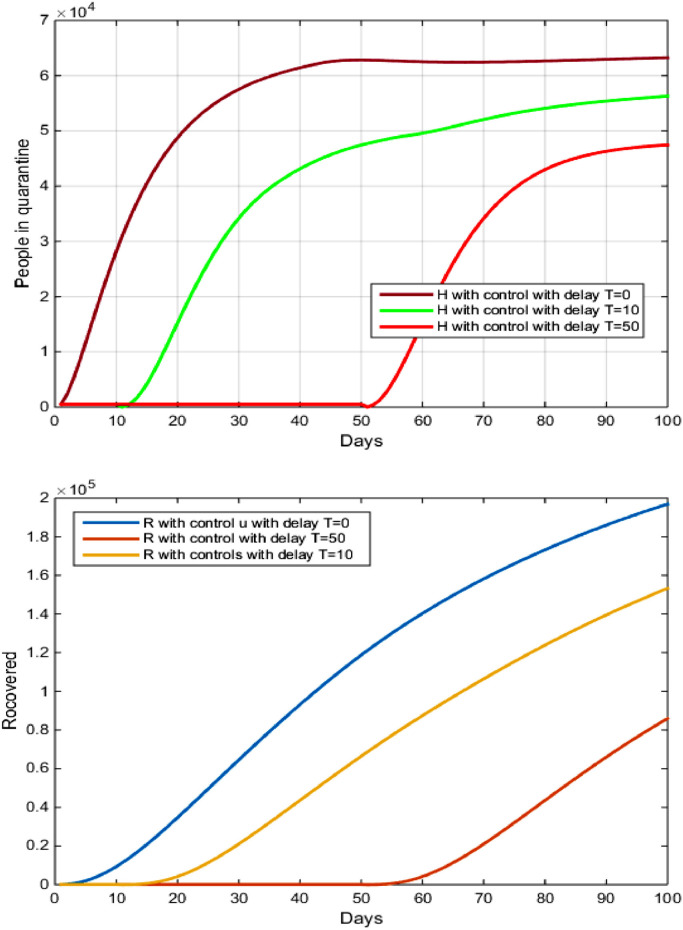
From Fig. 4 and Table 2 and 3, Delays in implementing the strategy to guide, educate and protect against COVID-19 in Brazil had very serious consequences after the outbreak of the epidemic after the initial settlement. This has resulted in a large and recently accelerated spread of more than 370,000 cases of COVID 19 virus, and its results will be a delay in early detection, which reduces the number of people healed and has significantly increased the number of deaths in Brazil.

Fig. 4.

The evolution of the number of Recovered and infected in quarantine with and without control $u\left(t\right)$ and with delay.

This delay is not taking into account advice and measures of prevention in a real and serious way:

• •Not taking the disease seriously in Brazil.
• •Not to wearing medical masks while keeping the hand clean, while reducing handshake.
• •Some consider this a regular virus, just like any other seasonal flu.
• •Not leaving a safe distance between him and the affected person.

In Fig. 2 shows that the number of recovered from the disease decreased negatively, we notice that after 100 days the number of recovered decreased From $1.01\times {10}^4$ to $8.11\times {10}^3$ after the delay of 10 days, while the decrease in the number of suscepetible increased from $1.01\times {10}^4$ to $6.29\times {10}^3$ after the delay of 50 days.

5.2. Strategy B: diagonsis and treatment

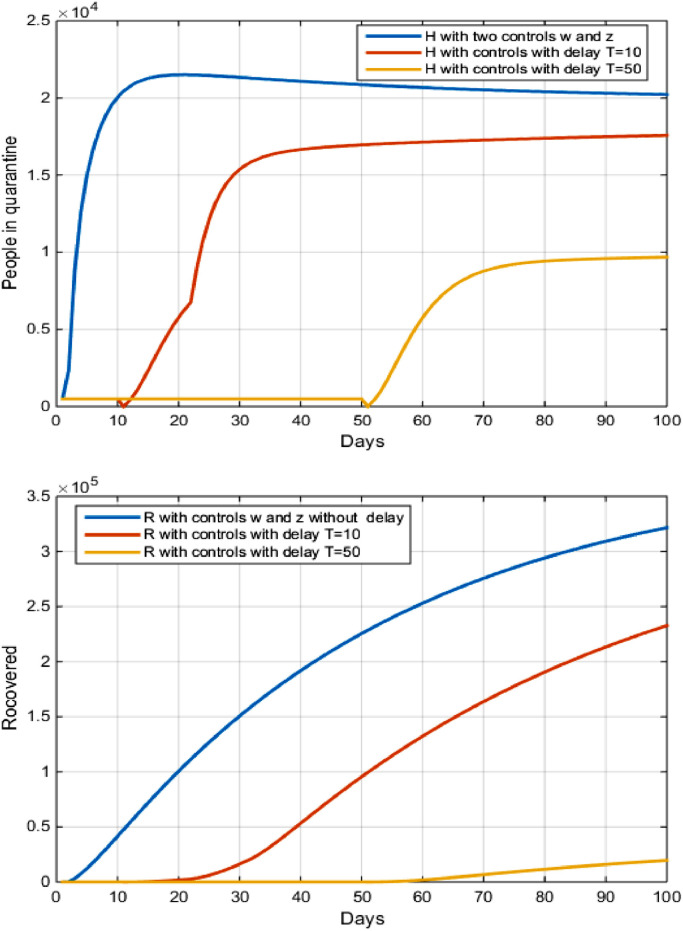
In his strategy, we combined two optimal controls $w\left(t\right)$ and $z\left(t\right)$.

In Fig. 5 and Tables 2 and 3 showed that the number of recovered from the disease decreased negatively, we noticed that after 100 days the number of recovered decreased From $1.01\times {10}^4$ to $8.11\times {10}^3$ after the delay of 10 days, while the decreased in the number of suscepetible increased from $1.01\times {10}^4$ to $6.29\times {10}^3$ after the delay of 20 days. We explained these results by the following: whenever the delay in the application of the strategy of surveillance and diagnosis of expatriates in Brazil from endemic countries such as Italy is a model of the fact that the first infected with Brazilian citizen came from Italy, with a diagnosis of his health and placing it under sanitary control for a period of at least 14 days. This has led to the massive spread of the virus in all regions of Brazil.

Fig. 5.

The evolution of the number of Recovered and infected in quarantine with and without control $w\left(t\right)$ and $z\left(t\right)$ and with delay.

5.3. Strategy C: quarantine and treatment

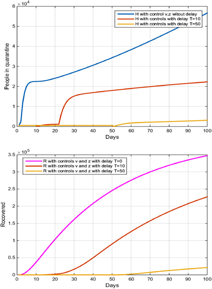
For This strategy we combined two controls $v\left(t\right)$ and $z\left(t\right)$.

In Fig. 6 and Tables 2 and 3 and showed that the number of recovered from the disease decreased negatively, we notice that after 100 days the number of recovered decreased From $8.1\times {10}^4$ to $4.08\times {10}^5$ after the delay of 10 days, while the decreased in the number of suscepetible increased from $8.1\times {10}^5$ to $6.72\times {10}^3$ after the delay of 50 days. We clarify these results by the following: The delay in implementing the quarantine strategy for infected with COVID-19, whether inside hospitals or at home in Brazil, and has led to a spread widespread in all regions of Brazil, where the number of people infected now exceeds 370,000 cases of infection of COVID-19.

Fig. 6.

The evolution of the number of Recovered and infected in quarantine with and without control $v\left(t\right)$ and $z\left(t\right)$ and with delay.

5.4. Strategy D: quarantine and diagnosis and monitoring with treatment

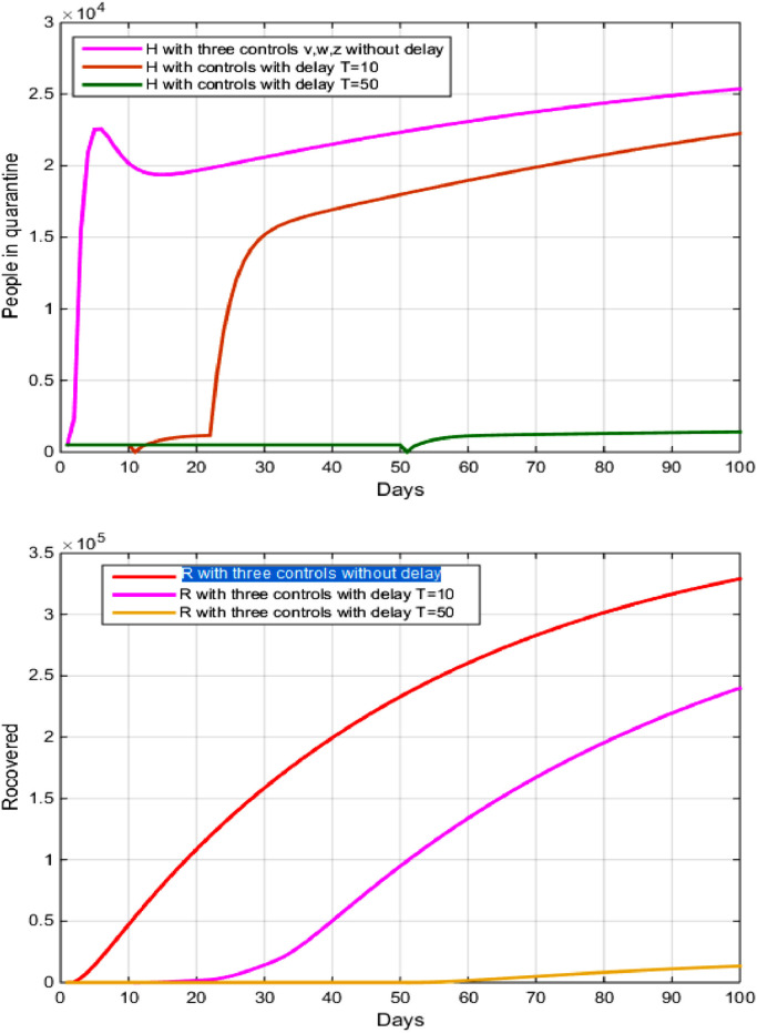
To use this optimal strategy, we combine between the optimal controls $v\left(t\right),w\left(t\right)$ and $z\left(t\right)$

From Fig. 7 , and depending on the values in Table 2, we note that the longer the delay in serious use and rapid interaction to reduce the spread of the virus. Fig. 4 shows that the number of people recovering from the disease decreased negatively and we notice that after 150 days the number of people recovered decreased From $4.56\times {10}^5$ to $3.17\times {10}^5$ after the delay of 10 days, while the decrease in the number of people recovered increased from $4\times {10}^5$ to $3.57\times {10}^3$ after the delay of 50 days.

Fig. 7.

The evolution of the number of recovered and hospitalization with and without controls with delay.

This decrease is due to several factors, including (Figs. 6 and 7 ):

• •The delay in schools closure in Brazil.
• •The delay in closing airports and ports in a timely manner in Brazil.
• •The delay in suspending air, land and sea travels from Brazil to affected countries.
• •The delay closure of schools, universities in Brazil.
• •The delay in applying precautionary, preventive and strict measures when receiving travelers to Brazil.
• •The tolerance of others in the passage of passengers through airports in some countries
• •The delay in diagnosis of infected cases, especially as symptoms do not appear in the disease’s incubation period.
• •The delay in applying total quarantine among patients increases the spread of the disease in all over Brazil.

5.5. Cost-effectiveness analysis

In this section, we analyze the profitability of the previous three scenarios and strategies by comparing these two control strategies to determine the most profitable strategy. Following the method applied in several studies [29], [30], [31], we assess costs using the differential cost-effectiveness (ICER). This ratio used compare the differences between costs and health outcomes of two competing intervention strategies.

The ICER is defined as the quotient of the difference in costs in strategies $i$ and $j,$ by the difference in infected averted in strategies $i$ and $j$ $(i,j\in \{1,2,3,4\left\}\right).$

Given two competing strategies (1) and (2), where strategy (2) has higher effectiveness than strategy (1) $\left(TA\right(2)>TA(1)$), the $ICER$ values are calculated as follow:

$$ICER\left(1\right)=\frac{TC\left(1\right)}{TA\left(1\right)}$$

$$ICER\left(2\right)=\frac{TC\left(2\right)-TC\left(1\right)}{TA\left(2\right)-TA\left(1\right)}$$

where the total costs $\left(TC\right)$ and the total cases averted $\left(TA\right)$ are defined, during a given period for strategy i for $i=1,2,3,4$ by:

$$\begin{array}{ccc}\hfill TC\left(i\right)& =& \underset{0}{\overset{T}{\int }}({\beta }_{1}u\left(t\right)\frac{S\left(t\right)E\left(t\right)}{N}+{\beta }_{2}u\left(t\right)\frac{S\left(t\right)I\left(t\right)}{N}\hfill \\ & & +v\left(t\right)\left(I\right(t)+D(t\left)\right)+z\left(t\right)H\left(t\right))dt\hfill \end{array}$$

$$\begin{array}{ccc}\hfill TA\left(i\right)& =& \underset{0}{\overset{T}{\int }}\left(E\right(t)+I(t)+C(t)+H(t\left)\right)\hfill \\ & & -(E^{*}\left(t\right)+I^{*}\left(t\right)+C^{*}\left(t\right)+H^{*}\left(t\right)))dt\hfill \end{array}$$

while $(E^{*}\left(t\right)+I^{*}\left(t\right)+C^{*}\left(t\right)+H^{*}\left(t\right))$ is the optimal solution associated to the optimal control $(u^{*},v^{*},w^{*},Z^{*})$ Using the simulation results and we ranked, in the Table 3 our control strategies in order of increased numbers of averted infections.

Strategy I is compared with strategy J with respect to increased effectiveness, in reference to Table 4. So (Table 4 ):

$$ICER\left(2\right)=\frac{TC\left(2\right)}{TA\left(2\right)}=\frac{1.57\times {10}^6}{4.82\times {10}^7}=0.032$$

$$ICER\left(3\right)=\frac{TC\left(3\right)-TC\left(2\right)}{TA\left(3\right)-TA\left(2\right)}=\frac{3.05\times {10}^6-1.57\times {10}^6}{4.85\times {10}^7-4.82\times {10}^7}=4.93$$

Table 4.

Total costs and total averted infections for strategies 1–4.

Strategy	Total averted infections (TA)	Total cost (TC)
4	$5.24\times {10}^7$	$1.94\times {10}^6$
3	$4.85\times {10}^7$	$3.05\times {10}^6$
2	$4.82\times {10}^7$	$1.57\times {10}^6$
1	$4.52\times {10}^7$	$5.92\times {10}^5$

Since $ICER\left(2\right)<ICER\left(3\right),$ then strategy 3 is less effective than strategy 1. Therefore, strategy 2 is excluded from the set of alternatives.

Next, strategy 2 is compared to strategy 4. The ICER values for strategy 4 and strategy 2 are calculated below:

$$ICER\left(2\right)=\frac{TC\left(2\right)}{TA\left(2\right)}=\frac{1.57\times {10}^6}{4.82\times {10}^7}=0.032$$

$$ICER\left(4\right)=\frac{TC\left(4\right)-TC\left(2\right)}{TA\left(4\right)-TA\left(2\right)}=\frac{1.94\times {10}^6-1.57\times {10}^6}{5.24\times {10}^7-4.82\times {10}^7}=0.08$$

Since $ICER\left(2\right)<ICER\left(4\right),$ then strategy 4 is less effective than strategy 2. Therefore, strategy 2 is excluded from the set of alternatives.

Next, strategy 2 is compared to strategy 1. The ICER values for strategy 2 and strategy 1 are calculated below:

$$ICER\left(2\right)=\frac{TC\left(2\right)}{TA\left(2\right)}=\frac{1.57\times {10}^6}{4.82\times {10}^7}=0.032$$

$$ICER\left(1\right)=\frac{TC\left(1\right)-TC\left(2\right)}{TA\left(1\right)-TA\left(2\right)}=\frac{5.92\times {10}^5-1.57\times {10}^6}{4.52\times {10}^7-4.82\times {10}^7}=32.6$$

Since $ICER\left(2\right)<ICER\left(1\right),$ then strategy 1 is less effective than strategy 2. Therefore, strategy 2 is excluded from the set of alternatives.

Therefore, the conclusion is that strategy 1 (awarness campaigns to protect potential individuals infected with the virus, prevent contact with people infected with COVID-19 and with hospital quarantine for the infected) is the most effective strategy as previously mentioned by the proportions.

6. Conclusion

In this paper, we introduced a mathematical model $S{I}_{W}ICHR$ of kouidere et al, that described the spread of COVID-19 virus in Brazil. We divided the population denoted by $N$ into six compartments, susceptible population Brazil $S,$ the infected without symptoms $I_W,$ the infected with symptoms $I,$ the infected with complications $C,$ the number of people who have been quarantined in hospitals $H$ and recovered $R$. We analyzed a mathematical model and the local and the global stability of COVID-19 free equilibrium and COVID-19 endemic equilibrium are obtained. We also studied the sensitivity analysis of the model parameters to know the parameters that have a high impact on the reproduction number $R_0$. In addition, in order to minimize the number of infected and infected with several complications and number of people in guarantine. We also introduced four controls which, respectively, represent sensitization, prevention, quarantine, diagnosis, monitoring, treatment and psychological support with follow-up. We also studied the optimal control with delay which represents measuring the extent of interaction with the means of treatment or awareness campaigns. that if preventive and proactive measures are implemented, such as awareness-raising and quarantine campaigns in all overe Brazil, the spread of the COVID-19 epidemic will be reduced, thus the number of people infected with the virus and the number of deaths will be reduced. We applied the results of the control theory and we managed to obtain the characterizations of the optimal controls. The numerical simulation of the obtained results showed the effectiveness of the proposed control strategies.

Funding source

None.

Ethical approval

Approval was not required.

CRediT authorship contribution statement

Abdelfatah Kouidere: Writing - original draft, Writing - review & editing. Driss Kada: Writing - original draft, Writing - review & editing. Omar Balatif: Writing - original draft, Writing - review & editing. Mostafa Rachik: Writing - original draft, Writing - review & editing. Mouhcine Naim: .

Declaration of Competing Interest

The authors declare that they have no conflict of interests.

References

- 1.World Health Organization. who.int/csr/don/12-january-2020-novel-coronavirus-china.
- 2.World Health Organization. who.int/emergencies/diseases/novel-coronavirus-2019.
- 3.World Health Organization. who.int/health-topics/coronavirus/laboratory-diagnostics-for-novel-coronavirus.
- 4.Middle east respiratory syndrome coronavirus (MERS-CoV) – the Kingdom of Saudi Arabia. 2019. Who.int/csr/don/05-december-2019-mers-saudi-arabia/.
- 5.Kouidere A., Balatif O., Ferjouchia H., Boutayeb A., Rachik M. Optimal control strategy for a discrete time to the dynamics of a population of diabetics with highlighting the impact of living environment. Discrete Dynamics in Nature and Society. 2019 [Google Scholar]; Article ID 5949303
- 6.Middle East respiratory syndrome coronavirus (MERS-CoV) Summary of Current Situation 21 July 2017.
- 7.Middle east respiratory syndrome coronavirus (MERS-CoV) – Qatar, 26 december 2019, http://www.who.int/csr/don/26-december-2019-mers-qatar.
- 8.Chen T., Rui J., Wang Q.. A mathematical model for simulating the phase-based transmissibility of a novel coronavirus. infect dis poverty. 2020. 9, 24, doi: 10.1186/s40249-020-00640-3. [DOI] [PMC free article] [PubMed]
- 9.Kucharski A.J.. Early dynamics of transmission and control of COVID-19: a mathematical modelling study. PMID: 32171059. doi: 10.1016/S1473-3099(20)30144-4. [DOI] [PMC free article] [PubMed]
- 10.Balatif O., Khajji B., Rachik M. Mathematical modeling, analysis, and optimal control of abstinence behavior of registration on the electoral lists. Discrete Dyn Nat Soc Vol. 2020;Article ID 9738934:12. doi: 10.1155/2020/9738934. [DOI] [Google Scholar]
- 11.Pontryagin L.S., Boltyanskii V.G., Gamkrelidze R.V., Mishchenko E.F. Wiley; New York, NY, USA: 1962. The mathematical theory of optimal processes. [Google Scholar]
- 12.Fleming W.H., Rishel R.W. Springer; New York, NY, USA: 1975. Deterministic and stochastic optimal control. [Google Scholar]
- 13.Novel coronavirus (2019-nCoV). https://www.who.int/docs/default-source/coronaviruse/situation-reports/20200315-sitrep-55-COVID-19.pdfsfvrsn=33daa5cb_8.
- 14.Novel coronavirus (2019-nCoV) technical guidance: Early investigations. who.int/emergencies/diseases/novel-coronavirus-2019/technical-guidance/early-investigations.
- 15.Boyce W.E., DiPrima R.C. John Wiley & Sons; New York: 2009. Elementary differential equations and boundary value problems. [Google Scholar]
- 16.Wang H., Wang Z., Dong Y. Phase-adjusted estimation of the number of coronavirus disease 2019 cases in Wuhan. China Cell Discov. 2020;6:10. doi: 10.1038/s41421-020-0148-0. [DOI] [PMC free article] [PubMed] [Google Scholar]
- 17.Al-Asuoad N., Rong L., Alaswad S., Shillo M.. Mathematical model and simulations of MERS outbreak: predictions and implications for control measures. 2016. 5(2).
- 18.Birkhoff G., Rota G.C. 4th ed. JohnWiley & Sons; New York: 1989. Ordinary differential equations. [Google Scholar]
- 19.The Food and Agriculture Organization of the United Nations (FAO), Coronavirus disease (COVID-19) outbreak, http://www.fao.org/2019-ncov/en/.
- 20.COVID-19 Overview, https://www.coronatracker.com/analytics/. 2020a.
- 21.World health organization. SARS virus. https://www.who.int/ith/diseases/sars/en/.
- 22.Choi S.C., Ki M.. Estimating the reproductive number and the outbreak size of novel coronavirus disease (COVID-19) using mathematical model in Republic of Korea. PMID: 32164053. doi: 10.4178/epih.e2020011. [DOI]
- 23.Kouidere A., Labzai A., Khajji B., Ferjouchia H., Balatif O., Boutayeb A., Rachik M. Optimal control strategy with multi-delay in state and control variables of a discrete mathematical modeling for the dynamics of diabetic population. Commun Math Biol Neurosci. 2020;2020 doi: 10.28919/cmbn/4486. [DOI] [Google Scholar]; Article ID 14 ISSN: 2052-2541
- 24.World Health Organization. https://experience.arcgis.com/experience/685d0ace521648f8a5beeeee1b9125cd. 2020b.
- 25.Kouidere A., Khajji B., El A., Balatif O., Rachik M. A mathematical modeling with optimal control strategy of transmission of COVID-19 pandemic virus. Commun Math Biol Neurosci. 2020;2020 doi: 10.28919/cmbn/4599. [DOI] [Google Scholar]; Article ID 24 ISSN: 2052-2541
- 26.Lekdee N., Sirisubtawee S., Koonprasert S. Bifurcations in a delayed fractional model of glucose-insulin interaction with incommensurate orders. Adv Differ Equ. 2019;2019:318. [Google Scholar]
- 27.Li Y., Liu H., Yang R., Tang L. Dynamics in a diffusive phytoplankton-zooplankton system with time delay and harvesting. Adv Differ Equ. 2019;2019:79. [Google Scholar]
- 28.Sarkar A., Mondal J., Chatterjee S. Controlling self-excited vibration using acceleration feedback with timedelay. Int J Dyn Control. 2019;7:1521–1531. [Google Scholar]
- 29.Silva C.J., Maurer H., Torres D.F.M. Optimal control of a tuberculosis model with state and control delays. Math Biosci Eng. 2017;14(1):321–337. doi: 10.3934/mbe.2017021. [DOI] [PubMed] [Google Scholar]
- 30.Khajji B., Kada D., Balatif O., Rachik M. A multi-region discrete time mathematical modeling of the dynamics of COVID-19 virus propagation using optimal control. J Appl Math Comput. 2020 doi: 10.1007/s12190-020-01354-3. [DOI] [PMC free article] [PubMed] [Google Scholar]
- 31.Khan M.A., Shah S.W., Ullah S., Gomez-Aguilar J.F. A dynamical model of asymptomatic carrier zika virus with optimal control strategies. Nonlinear Anal Real World Appl. 2019;50:144–170. [Google Scholar]
- 32.Bonyah E., Khan M.A., Okosun K.O., Gomez-Aguilar J.F. Modelling the effects of heavy alcohol consumption on the transmission dynamics of gonorrhea with optimal control. Math Biosci. 2019;309:1–11. doi: 10.1016/j.mbs.2018.12.015. [DOI] [PubMed] [Google Scholar]
- 33.Ullah S., Khan M.A., Gomez-Aguilar J.F. Mathematical formulation of hepatitis B virus with optimal control analysis. Optim Control Appl Methods. 2019;40(3):529–544. [Google Scholar]
- 34.Bentout S., Chekroun A., Kuniya T. Parameter estimation and prediction for coronavirus disease outbreak 2019 (COVID-19) in algeria. AIMS Public Health. 2020;7(2):306–318. doi: 10.3934/publichealth.2020026. [DOI] [PMC free article] [PubMed] [Google Scholar]
- 35.Bani-Yaghoub M., Gautam R., Shuai Z., van den Driessche P., Ivanek R. Reproduction numbers for infections with free-living pathogens growing in the environment. J Biol Dyn. 2012;6(2):923940. doi: 10.1080/17513758.2012.693206. [DOI] [PubMed] [Google Scholar]
- 36.Driessche P.V., Watmough J. Reproduction numbers and sub-threshold endemic equilibria for compartmental models of disease transmission. Math Biosci. 2002;180:2948. doi: 10.1016/s0025-5564(02)00108-6. [DOI] [PubMed] [Google Scholar]
- 37.LaSalle J.P. Regional conference series in applied mathematics. Vol. 25. SIAM; Philadelphia, PA, USA: 1976. The stability of dynamical systems. [Google Scholar]
- 38.Gumel A.B., Shivakumar P.N., Sahai B.M. A mathematical model for the dynamics of HIV-1 during the typical course of infection. Nonlinear Anal. 2001;47(3):17731783. [Google Scholar]
- 39.Karrakchou J., Rachik M., Gourari S. Optimal control and infectiology: application to an HIV/AIDS model. Appl Math Comput. 2006;177(2):807818. [Google Scholar]
- 40.Chitnis N., Cushing J.M., Hyman J.M. Bifurcation analysis of a mathematical model for malaria transmission. SIAM J Appl Math. 2006;67(1):2445. [Google Scholar]