Abstract
The occupant density in buildings is one of the major and overlooked parameters affecting the energy consumption and virus transmission risk in buildings. HVAC systems energy consumption is highly dependent on the number of occupants. Studies on the transmission of COVID-19 virus have indicated a direct relationship between occupant density and COVID-19 infection risk. This study aims to seek the optimum occupant distribution patterns that account for the lowest number of infected people and minimum energy consumption.
A university building located in Tehran has been chosen as a case study, due to its flexibility in performing various occupant distribution patterns. This multi-objective optimization problem, with the objective functions of energy consumption and COVID-19 infected people, is solved by NSGA-II algorithm. Energy consumption is evaluated by EnergyPlus, then it is supplied to the algorithm through a co-simulation communication between EnergyPlus and MATLAB. Results of this optimization algorithm for 5 consequent winter and summer days, represent optimum occupant distribution patterns, associated with minimum energy consumption and COVID-19 infected people for winter and summer.
Building air exchange rate, class duration, and working hours of the university, as the COVID-19 controlling approaches were studied, and promising results have been obtained. It was concluded that an optimal population distribution can reduce the number of infected people by up to 56% and energy consumption by 32%. Furthermore, it was concluded that virtual learning is an excellent approach in universities to control the number of infections and energy consumption.
Keywords: Occupant distribution, Building energy simulation, Building energy performance, Viral infection rate, Airborne transmission, COVID-19
Nomenclature
- S
Sensible Generated Heat (W)
- M
Metabolic Rate (W)
- T
Temperature (°C)
- RH
Relative Humidity
Mass Flowrate (kg/s)
- L
Heat Load of Individuals (W)
- h
Enthalpy (J/kg)
- fcl
Ratio of Clothes Surface to the Body Surface (−)
- Icl
Thermal Resistance of the Garment (clo)
- hcl
Convective Heat Transfer Coefficient (W/m2.K)
- P
Partial vapor Pressure (Pa)
- IR
Inhalation Rate (m3/hr)
- ERq
Quanta Emission Rate (quanta/hr)
- IVRR
Virus Elimination Rate (1/hr)
- t
Exposure Time (hr)
- n
Quanta Concentration (quanta/m3)
- R
Virus Infection Risk (−)
- T
Total Exposure Time (hr)
- S
Number of Present Occupants (−)
- In
New Infected People (−)
- W
Heat Loss (W)
- V
Volume (m3)
- Csettling
Virus Settling Rate (1/hr)
- Cinactivation
Virus Inactivation Rate (1/hr)
Subscripts
- min
Minimum
- SA
Supply Air
- out
Leaving Air
- zone
Thermal Zone Air
- cl
Clothes
- c
Cooling
- h
Heating
- x
Number of Occupants
- r
Radiation
Abbreviations
- NSGA-II
Nondominated Sorting Genetic Algorithm II
- HVAC
Heating, Ventilation and Air Conditioning
- COVID-19
Corona Virus Disease 2019
- PMV
Predicted Mean Vote
- AER
Air Exchange Rate (1/hr)
- PTAC
Packaged Terminal Air Conditioner
- E
Energy
1. Introduction
Climate change, environmental issues, and the energy crisis has made energy management more important than before. Since buildings account for 30%–40% of society's energy demand, they have the potential to alleviate the worldwide energy-related issues [1]. In this context, according to the United States Energy Information Agency (EIA) [2], HVAC systems are responsible for about 42% of the electricity consumption in commercial buildings in the U.S. The presence of occupants in buildings is one of the most important parameters in the buildings that affect the energy consumption of HVAC systems. There are, however, other dominant parameters for the energy consumption of HVAC systems, but studies show that controlling the attendance time of people can be effective in managing building energy consumption [[3], [4], [5]]. Therefore, an optimum occupant presence schedule may significantly reduce the overall energy consumption of buildings.
Occupants generate heat by their activity in buildings, which is added to the overall heat load of the buildings. This increases the energy consumption of cooling systems. Conversions in weather conditions such as solar radiation, wind speed and direction, and air temperature are the main parameters that determine the energy consumption of the building. Therefore, at different times of the day, HVAC systems would require various amount of energy to provide a desirable condition for occupants. Hence, by knowing the climatic conditions, it is possible to adjust the attendance of occupants effectively, so that fewer people would be present in the times that HVAC systems require more energy, and conversely, more people would exist in the building when HVAC systems require less energy. Implementation of this strategy in buildings can significantly reduce the energy consumption of the building, without using additional equipment or renewable energy systems. This strategy, however, is more effective in public places e.g. stores, offices, universities, service providers, etc.
Another major objective of this study is to control the infection risk of COVID-19 and other respiratory viruses. Controlling the probability of contact is the most important strategy for controlling respiratory viruses. The Coronavirus is transmitted among people through inhalation and exhalation and also by direct contact with infected objects [6]. As the population density in a building increases, the probability of the virus transmission in both ways increases, and as a result, the number of infected people with the virus increases. Therefore, by recognizing virus transmission parameters, the probability of virus transmission in the building can be estimated and, it would be possible to provide an optimal occupant distribution pattern, which has the lowest number of infected people.
Optimization algorithms are one of the most effective tools in energy modeling problems to characterize a global optimum value for a parameter as an objective function. These problems can inherently be single-objective or multi-objective optimization problems along with some constraints. In this context, metaheuristic algorithms are intelligent solvers especially used for solving complex optimization problems [7]. Most of the building optimization problems are multi-objective problems and metaheuristic algorithms are usually utilized to solve these problems.
The most famous multi-objective algorithms are NSGA-II [8], MOPSO [9], and SPEA2 [10]. Several applications of these algorithms in building optimization problems can be found in previous literature [1,[11], [12], [13], [14], [15]].
The extremely varied and unpredictable specifications of occupants in buildings have made them complex to model and being ignored in most of the previous building energy simulation studies. This simplification creates a huge inaccuracy between the actual energy consumption and the simulated one. Fortunately, in recent years, numerous studies have been conducted to understand occupant behavior in buildings. Huila et al. [16] and Menezes et al. [17] compared the accuracy of building energy simulation with and without considering the presence of people inside the building. The results show that considering the occupants in the simulation generates more accurate results. Dedesco et al. [18] studied the effect of various occupant-related parameters e.g. number of occupants and presence duration of occupants on the energy consumption in hospital rooms. Rio et al. [19] have proposed a model for estimating the presence of occupants in a building to create an accurate energy simulation using data mining techniques. In order to find the best population density in a building, Kang et al. [20] studied the effect of occupant density on 105 buildings and derived a direct relationship between the number of occupants and the building's energy consumption. Li and Yao [21], and Want et al. [22], considering the occupants, implemented machine learning techniques in modeling and predicting the energy consumption of buildings and concluded that occupant's presence and behaviors are one of the most determinant factors in energy consumption of buildings. Sun et al. [23] proposed a framework for data-driven occupant behavior analytics in residential buildings and concluded that occupant's effect on a building's energy consumption is significant, whether it's a residential or a commercial building. Jami et al. [24] adopted energy conservation measures in a student dormitory in Tehran by considering the occupant behaviors. They concluded that the accuracy of the energy conservation measures is highly associated with considering occupant energy behavior.
Rising the occupant density in a building leads to an increase in the physical contact between the people as well as breathing more common air and consequently, increasing the number of infected people in the building. Some research projects have been devoted to investigating the effect of occupant density and comfort conditions on the virus transmission rate [25,26]. In a recent study, Horo et al. [27] investigated the microbial dynamics and occupants interactions to understand the effect of building characteristics e.g. architectural design parameters, indoor moisture content, temperature, and lighting level as well as the occupant density, on the microbial survivability in buildings. Sari et al. [28] examined the affecting factors of the virus spread in the building and concluded that the occupant density is one of the most important factors in virus transmission. Kossi et al. [29] also examined the effect of indoor air quality conditions and population of pupils on respiratory infection in Canadian schools and demonstrated the importance of occupant distribution. Zhan et al. [30] evaluated the impacts of environmental conditions on the transmission of COVID-19 and studied virus transmission in different conditions. Ronchi and Lovreglio [31] assessed the crowd modeling effects on the occupant exposures in the confined spaces and proposed EXPOSED crowd model, as an effective occupant presence model during pandemics. Guo et at [32]. compared different guideline approaches in HVAC operation during COVID-19 pandemic and concluded that maximizing the fresh air supply in HVAC systems is the most effective strategy to mitigate the COVID-19 infection risk. Wee MPH et al. [33] Evaluated different approaches to reduce the risk of COVID-19 transmission in a multibedded cohorted general ward setting and concluded that social distancing between patients is a must for this approach. Rahman et al. [34] also reported that social distancing and avoiding crowds are among the promising approaches to prevent transmission of respiratory viruses. Sun and Zhai [35] have suggested a prediction model for the airborne virus in confined spaces that takes into account the occupant density, ventilation rate, and the exposure time on the infection risk. They concluded that social distancing is a great approach to decrease the infection risk and also minimizes the required ventilation rate in buildings.
COVID-19 pandemic has had irreparable damage to the world. According to the World Health Organization, 1.3 million people have passed away worldwide until 16 November 2020. In addition to health problems, COVID-19 has either completely disabled various industries or caused millions of dollars in damage for them. Research activities in academia can greatly help to mitigate this vital issue. In this regard, this virus must be precisely studied in different aspects to better understand the ways of minimizing the casualties and controlling the pandemic. Although various research studies have been conducted about COVID-19, due to the novelty of this virus, there hasn't been enough time to comprehensively study the virus. Therefore, previous literature lacks an investigation of various factors that affect the transmission of COVID-19. This paper is set up to fill the gap in the related context and aims to better understand the characteristics of the virus to help control the pandemic along with energy consumption. On the other hand, Countless parameters are affecting the HVAC system's energy consumption and COVID-19 infection risk in buildings which can be evaluated to conclude precise results e.g. occupant behavior, facial mask effect, occupant distribution, air exchange rate, building geometry, variable air exchange rate, working hours of building, exposure duration, occupant's activity level, clothing, etc. [36]. However, in this paper, the most dominant factors i.e. the effects of different occupant distribution, air exchange rates, working hours, and class duration on the HVAC system's energy consumption and the number of infected people with COVID-19 virus are investigated. Examining different occupant distributions lead to provide optimal schedules for the occupants in the buildings to align the internal load with the climatic conditions and to prevent crowding. By considering the energy consumption and the number of infected people as the objective functions, the multi-objective optimization problem has been solved by linking the virus infection risk and the EnergyPlus [37] outputs with the NSGA-II algorithm [8]. Simulations were conducted in 5 consequent days in winter and summer for a case study university building in Tehran. Furthermore, the effects of ventilation rate, working hours of the university, and the class durations on the HVAC system's energy consumption and the number of infected people with COVID-19 have been precisely investigated to propose the best approaches for controlling the number of infected people and decrease the energy consumption in buildings.
2. Material and methods
In this multi-objective optimization problem, energy consumption and the number of infected people with COVID-19 are intended to be simultaneously minimized. Therefore, instead of a unique optimum solution, a set of non-dominated solutions are being resulted. The decision variables of this problem are the number of occupants at different hours of the day. Therefore, the decision variables are discrete values from 0 to the maximum occupant capacity of the building. Various optimization algorithms have been developed to solve these sorts of problems [[8], [9], [10],38]. Among the existing optimization algorithms, NSGA-II stands out as a perfect solver, which does not get stuck in a local optimum and performs greatly in discrete problems. Besides, NSGA-II provides a well-distributed set of non-dominated solutions. The widespread use of NSGA-II in building optimization problems is a prove of these facts [[11], [12], [13],15]. Therefore, NSGA-II is adopted for this work to solve the optimization problem and find the optimum daily occupant distribution.
In the first step of this algorithm, a random set of occupant distribution pattern, that is called chromosomes is created in the size of the algorithm population. Chromosomes are a series of solutions (in this problem, different values of occupant distribution pattern) that arrange sequentially. In the next stage, these randomly generated chromosomes are evaluated by the predetermined cost functions, which are the number of COVID-19 infected people and energy consumption. Since this problem is a dual-objective optimization problem, each chromosome holds two values associated with two objective functions. So, these chromosomes cannot be compared regularly. For comparing these chromosomes, nondominated solutions are defined as:
“X1 dominates X2, if and only if X1 is less than X2 in all values of the cost functions.”
Besides the domination comparison, another factor called crowding distance that indicates the amount of accumulation of answers at a single point of space is used as a second approach of evaluating solutions. In the solution space, if a chromosome is far from the others, it will have a more crowding distance value and makes the set of solutions out of integration, which is not desirable. This approach distinguishes the nondominated chromosomes and is stored to be used in the next iterations. After passing the initial iteration of this algorithm, it keeps doing this process again but this time instead of generating random solutions, the set of nondominated solutions of the previous iteration are being supplied to the algorithm. According to the predetermined proportions of crossover and mutation populations, a set of chromosomes are being randomly chosen from the main population.
Crossover and mutation operators, increase the exploration power of the algorithm. These operators modify the components of parent chromosomes and generate new sets of chromosomes that are called offspring (children). The crossover operator substitutes the components of a pair of answers. This substitution takes place in three ways: single point, double point, and uniform crossovers. In a single point crossover, the components of the chromosomes are cut off from a randomly selected point and are then substituted by each other. In a double point crossover, the components are cut off from two random points and are replaced by each other. In a uniform crossover, the components of a chromosome are multiplied by a random number between 0 and 1, and for another chromosome, the complement of this value is multiplied, and eventually, new chromosomes form by summarizing these two answers. In this way, the population of children is generated [8]. Another essential operator is mutation. This operator mutates the components of a chromosome, generating new chromosomes. For mutation, three operators i.e. swap, reversion, and insertion are utilized. Swap operator selects two random chromosome points and replaces them with each other to form a new chromosome. Reversion selects two random points in a chromosome and by reversing the order of the components between the two points, generates new chromosomes. The insertion operator selects two random chromosome points and the first component is transferred to the position before the second point. The selection of each of these operators for mutation is also considered randomly with equal probability.
The populations of crossover and mutation are generated by applying the relevant operators on these chromosomes. The crossover and mutation populations are also evaluated by the objective functions. Eventually, these populations together with the main population are merged and after performing comparisons, non-dominated chromosomes are separated in the amount of predetermined algorithm population size. This iterative process continues until the stopping conditions are met and a population of superior answers that have achieved the lowest values of the objective functions is obtained [39].
2.1. Energy simulation
The objective functions of this optimization problem are COVID-19 infected people count and HVAC system energy consumption, which needs to be simultaneously minimized. COVID-19 infected people count is highly dependent on the occupant density, so the optimization algorithm seeks an occupant distribution pattern that the infected people through a day is the lowest. Energy consumption as one of the objective functions is minimized by evaluating different occupant distribution patterns within a day in the building. Occupants in the building generate heat which is added to the heat load of the building. Therefore, occupant density affects the HVAC system's energy consumption. To evaluate the energy consumption of different occupant distribution patterns, EnergyPlus has been used. By importing building parameters and weather conditions, this powerful software calculates the energy consumption of building in a fast and accurate way. Eq. (1) shows sensible heat which is generated by the occupants. In this equation, is the metabolic rate (W), is the zone air temperature (°C) and is the generated sensible heat (W) [40].
| (1) |
Latent heat () can also be easily calculated as follow:
| (2) |
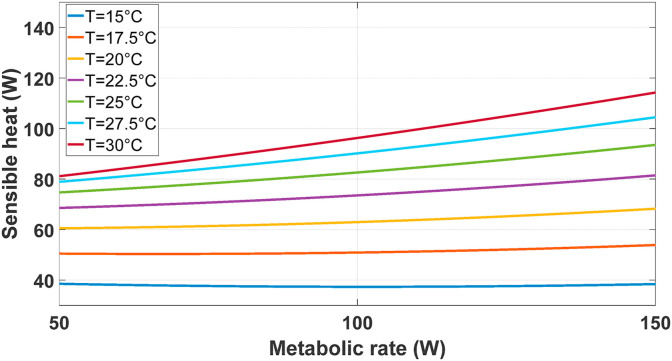
Fig. 1 shows generated heat by individuals in a university environment based on the temperature of the heat zone, calculated by ASHRAE standard 2004–2005 [41].
Fig. 1.
Heat generation rate by occupants in the classrooms for different zone temperatures.
Eq. (3) shows the amount of cooling/heating energy that the air conditioning systems transfer to the zones [40]. In this regard, is the mass flow rate of air that is sent through this system to the thermal zones (kg/s), is the enthalpy of leaving air from the system (J/kg) and is the enthalpy of thermal zone air. is referring to the constant relative humidity condition which is the minimum relative humidity of the air within the zones.
| (3) |
2.2. Co-simulation
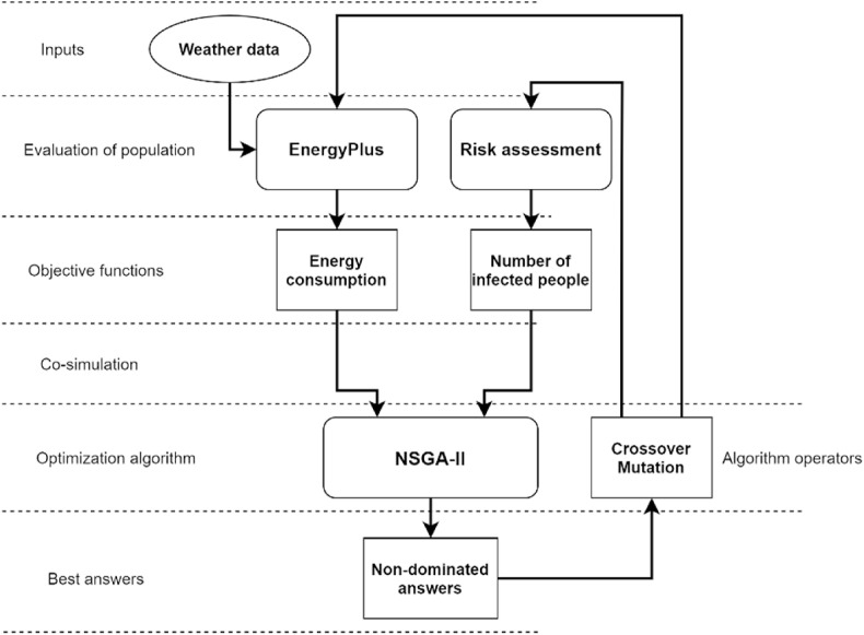
This problem aims to find the optimum occupant distribution through a day in the building to minimize the objective functions (i.e. energy consumption and COVID-19 infected people). To do so, a connection between the objective functions and the optimization algorithm should be made. COVID-19 infection equations are implemented in MATLAB and the other objective function, which is the energy consumption is evaluated by EnergyPlus. The communication between the EnergyPlus and MATLAB is established using EnergyPlus Co-simulation Toolbox [42]. First, a set of different occupant distribution is evaluated by both objective functions. The amounts of objective functions for each occupant distribution pattern that is stored in a chromosome are evaluated by NSGA-II algorithm and the non-dominated chromosomes form a new set of occupant distribution patterns. In this stage, the next generation of children is generated by performing crossover and mutation operators on the non-dominated solutions. This iterative process keeps running until the stopping condition is met. Eventually, a set of non-dominated occupant distribution patterns that have the least amount of COVID-19 infected people and energy consumption, form a Pareto front. A general schematic of this process is presented in Fig. 2 .
Fig. 2.
The overall process of the optimization problem.
2.3. Thermal comfort
Fanger's thermal comfort model is utilized to determine the thermal comfort conditions of occupants in the building [43]. In this model, the PMV value is introduced as an indication for the thermal comfort conditions of occupants. A positive PMV value denotes a feeling of warmth and conversely, a negative PMV value indicates a feeling of coldness for occupants. Accordingly, the ideal PMV value would be 0. Eq. (4) is utilized to calculate PMV in the zones [44].
| (4) |
In this equation, is the metabolic rate (W) and is the latent heat load of individuals (W), which is again calculated by the following equation:
| (5) |
In this equation, in addition to the production capacity by the activity of individuals, heat loss from convection, radiation, and respiration is also considered, in which , , , , and are the rate of heat loss due to the performance of work (W), clothing surface, convective heat transfer coefficient (W/m2), The surface temperature of the clothes (°C), mean radiant temperature (°C), and the partial vapor pressure of the thermal zone (Pa), respectively. represents the ratio of the surface of the clothes to the surface of the body, which can be calculated by Eq. (6). In this equation, is the thermal resistance of the garment (clo).
| (6) |
2.4. COVID-19 infection risk
To calculate the risk of COVID-19 infection, the number of floating virus particles in the room is required. For this purpose, first, the calculation process of the number of virus particles in space is discussed. Riley et al. [45]. proposed a model (known as Wells-Riley model), which shows the exponential increase of the number of newly infected people with time for steady-state quanta levels. Later, Gammaitoni and Nucci [46] represented an upgraded model for Wells-Riley model, which is based on the change in quanta levels through time in confined spaces. This model has successfully been used in supermarkets [47], airplanes [48], and cars [49]. The differential equations in the Gammaitoni model are solved considering initial conditions to estimate the quanta concentration in a confined space at the time . Some simplifying assumptions are considered to derive a proper equation to evaluate the quanta concentration in the building, which are as follow: the quanta emission rate remains constant, the period of the disease is longer than the time scale of the model, and the droplets are instantaneously distributed in the area [46,47]. These simplifying assumptions form Eq. (7). This equation shows the number of virus quanta in the space by considering affecting various parameters. Quanta is a definition used for infectious airborne particles. In this equation, is the quanta concentration, which is simply the ratio of quanta particles to the volume of the building (quanta/m3), is the volume of the building (m3), is the number of infected people in the building, is the virus particles that are distributed in the space by each inhale and exhale which depends on the characteristics of the virus. Furthermore, represents the time of exposure of the affected people in the space (hour), is the initial concentration of the virus particles in the space and represents the virus elimination rate, which can be calculated by Eq. (8) [50]. In this equation, represents the air exchange rate of the space (hr−1), is a coefficient, representing the virus settlement (hr−1) and is the virus inactivation rate (hr−1).
| (7) |
| (8) |
Accordingly, the concentration of virus particles in the building can be calculated by considering the characteristics of the virus and the building properties. After calculating the virus concentration, infection risk can be calculated for non-infected people. Eq. (9) is utilized to calculate the virus infection risk [45]. In this equation, is the virus quanta concentration in space (quanta/m3) which is calculated by Eq. (7), represents the exposed time of the occupants (hr) and indicate the inhalation rate of people (m3/hr). These parameters can be used to obtain the infection risk of people in the building. Furthermore, the number of infected people can be estimated by Eq. (10). In this equation is the virus infection risk, is the number of present occupants in the building and is the number of newly infected people [51].
| (9) |
| (10) |
3. Problem definition
The non-dominated sorting genetic algorithm II (NSGA-II) has multiple adjustable parameters that need to be precisely determined to achieve the desired performance, comprising crossover proportion, mutation proportion, the population of chromosomes, and the number of iterations. Depending on the type of the optimization problem and the characteristics of the decision variables, these parameters have optimum values which can be obtained by performing several simulations and achieving suitable exploration and exploitation rates. There is not a certain value for these parameters and they vary by the characteristics of the problem. By running the algorithm several times, it has been realized that a crossover and mutation proportion of respectively 60% and 40% provides a suitable exploration and exploitation amount for this problem. Furthermore, it has been concluded that an algorithm population size of 100 makes a perfect balance between the performance and the speed of the algorithm. Running the algorithm with these parameters showed that after 20 iterations, no change is observed in the final answers and the solutions have been already inclined to an optimum value. The empirically obtained optimum values of these parameters are given in Table 1 .
Table 1.
Obtained optimum values for the optimization algorithm.
| Parameter | Quantity |
|---|---|
| Iterations | 20 |
| Algorithm population count | 100 |
| Crossover proportion | 60% |
| Mutation proportion | 40% |
This problem is a dual-objective optimization problem aiming at minimizing energy consumption and the number of infected people with COVID-19 virus. The following equations are the constitutive optimization equations and constraints.
| (11) |
| (12) |
| (13) |
| (14) |
Eq. (11) is stating the minimization of the infected people within 5 days. In this equation as the first objective function, is the total number of infected people with the virus through the considered period that must be minimized. is the number of infected people in a certain hour of and the occupant count of . is obtained by summarizing the infected people through the working hours of the day (i.e. 8 to 19 within 5 days). Eq. (12) represents the second objective function which is also a minimization statement. This objective function is denoting the total energy consumption of the HVAC systems as , which is a summation of cooling energy and heating energy in thermal zones. Cooling and heating energy consumptions also vary by the time () and the number of occupants (). Therefore, determines the different times of the day which has various climatic parameters (e.g. solar radiation, ambient temperature, and wind speed). on the other hand, is the decision variable of this optimization problem which determines the values for objective functions. Eqs. (13), (14) are the constraints of the optimization problem that represent the cumulative number of occupants in the building during a day as well as the minimum and the maximum number of occupants in each hour. So, this multi-objective optimization problem searches for the optimum solutions for the occupant distribution within a day, by considering the bounds of the occupant counts and the predetermined total number of present occupants. The final set of solutions will form a Pareto front, which represents the dispersion of solutions in the search space by considering the values of their objective functions.
3.1. Building
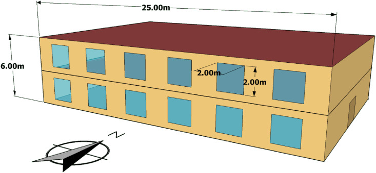
The case study building is a two-story university building designed by Sketchup 3D software. Fig. 3 shows the dimensions and orientation of this building. This building is considered to be located in Tehran, with a semi-arid climate and relatively high solar radiation [52]. Therefore, the utilization of solar energy is one of the most important parameters that determine the orientation of buildings in Tehran. Accordingly, most of the buildings in Tehran are north/south-oriented and so this building is considered to be oriented as north/south.
Fig. 3.
Dimensions and orientation of the case study university building.
This building has 24 windows and 2 exit doors. The general properties of the considered building are given in Table 2 . This building consists of 6 classrooms on each floor with a 48 m2 area, forming 12 classrooms at all. As a rule of thumb, approximately 2.5 m2 area is considered for each student and so 19.2 students will fit in each classroom, which by considering a teacher and rounding up, this number will rise up to 20 [53]. Therefore, the maximum number of present occupants in the building (by considering the formation of all classes) will be 240 people. Considering 5 permanent staffs working within the working hours, the maximum number of present people will be 245 people. It is assumed that the class durations are 1 h and each classroom forms 5 classes per day. Therefore, having 12 classes at all in the building, indicates that 60 classes with 1-h duration will be formed each day. Since the maximum number of present occupants in the building is 245 people, and each classroom forms 5 classes per day, total number of daily present people would be 1225 people. Referring to Iranian universities, the working hours of the building is assumed to be from 8 a.m. to a maximum of 8 p.m., so hereby, different chromosomes are the distribution of occupants ranging from 8 a.m. to 8 p.m.
Table 2.
Case study building properties.
| Parameters | Quantity |
|---|---|
| Stories | 2 |
| Windows | 24 |
| Gross area | 425 m2 |
| Height of walls | 3 m |
| Exit doors | 2 |
The building materials have been determined the same as an office building according to the standard regulations of ASHRAE material HOF 2005 [54] as well as the items used in Iran. The windows are double glazed with a single layer of air between the glasses and the doors are made of wood. Information on the specification of materials is collected in Table 3 . According to ANSI/ASHRAE 62–2 [55], the appropriate amount of the air exchange rate (AER) for HVAC systems in the universities is considered to be 3 hr−1.
Table 3.
Specifications of the building constructions.
| Building Construction | Components (Outside to inside) | Thickness (cm) | Thermal Conductivity (W/m.K) | Overall heat transfer coefficient (W/m2k) |
|---|---|---|---|---|
| External Wall | stucco | 2.5 | 0.6918 | 0.66 |
| Concrete | 20 | 1.7296 | ||
| Wall Insulation | 5.5 | 0.0432 | ||
| Gypsum | 1.27 | 0.16 | ||
| Internal Wall | Gypsum | 2 | 0.16 | 2.5 |
| Wall Air | 0.36 | 0.024 | ||
| Gypsum | 2 | 0.16 | ||
| Window | Clear Glass | 0.3 | 0.9 | 7.6 |
| Air | 0.3 | 0.024 | ||
| Clear Glass | 0.3 | 0.9 | ||
| Door | Wood | 5 | 0.15 | 3 |
| Ceiling | Lightweight Concrete | 10 | 0.53 | 1.37 |
| Air | 0.5 | 0.024 | ||
| Acoustic Tile | 2 | 0.06 | ||
| Roof | Roof Membrane | 0.95 | 0.16 | 0.23 |
| Roof Insulation | 21 | 0.049 | ||
| Metal Decking | 0.15 | 45 | ||
| Ground | Acoustic Tile | 2 | 0.06 | 0.74 |
| Air | 2 | 0.024 | ||
| Lightweight Concrete | 10 | 0.53 |
3.2. Internal loads
The metabolic heat generation of the occupants in a classroom is reported as an average of 150 W per person [41]. The insulation level of occupant's clothes is also determined to be variable for each season so that people in hot and cold seasons would have clothing insulation levels of 0.4 and 1.09 (clo), respectively [41]. Lightings are among the other major internal loads in this building. The appropriate level of lighting for the classrooms is 250 (lumens/m2) [56]. Therefore, to satisfy the favorable illumination rate for the occupants by taking into account the presence of people in different classes, the variable value of 5 (Watts/person) is considered. Other existing loads in the building are computers, printers, smart appliances, etc. These loads are divided into two groups of fixed and variable loads. The amount of considered fixed loads e.g. CCTV cameras, control systems, electronic doors, etc., which are listed in Table 4 , is 2000 Watts for whole thermal zones. Variable loads that depend on the number of people, including computers and laptops, is considered to be 100 Watts/person.
Table 4.
Building internal loads.
| Constant Loads | CCTV Cameras |
2000 W |
|---|---|---|
| Access Control systems | ||
| Electronic Doors | ||
| Security Computers | ||
| Public Use Electronics | ||
| Variable Loads | Student's Computers | 100 W/person |
| Laptops | ||
| Laboratory Equipment | ||
| Smart Board |
3.3. HVAC systems
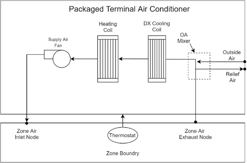
For the HVAC system, Packaged Terminal Air Conditioner (PTAC) is utilized to provide the required heating and cooling for the occupants. This system consists of cooling and heating coils, an outdoor air mixing system, and a blowing fan [40]. Fig. 4 represents a schematic of a PTAC air conditioning system.
Fig. 4.
Schematic of the PTAC air conditioning system [40].
The thermostats are adjusted by the thermal comfort conditions of the occupants, fixing the PMV value in the thermal zones in 0. Cooling coils, heating coils, and airflow are the decision variables that can interactively change to provide the determined PMV value. According to the World Health Organization's suggestions for the HVAC systems performance during COVID-19, demand-control ventilation controls that change the outdoor flowrate by the occupants should be disabled [57]. So, a constant airflow is considered for HVAC systems to comply with WHO's suggestions for controlling the COVID-19. Therefore, outside air's flowrate is considered to be 3 (hr−1).
3.4. Energy consumption
Thermostats are adjusted by the PMV of occupants and the HVAC systems are controlled according to these values. Setting the PMV value of 0 for HVAC systems will increase the sensitivity of the HVAC system's energy consumption on the occupant density and in consequence, the results of the optimization will be more contagious.
The presence of occupants at different hours of a day, makes electricity demand vary through these hours, so that the amount of generated heat by the occupants increases as the occupant density increases in thermal zones, leading to more energy consumption by the HVAC systems to establish thermal comfort. The simulations were conducted for two different periods of 5 consequent days in hot and cold seasons so that the effect of the occupant's presence in each season on the electricity consumption of HVAC systems, becomes evident.
3.5. Infection risk
To estimate COVID-19 infection risk in the building, the initial step is to calculate the virus quanta concentration in each hour. By knowing the required values of climate conditions, virus parameters, and the occupant's specifications, virus quanta concentration can be calculated by Eqs. (7), (8). To Calculate the number of already infected people () in Eq. (7), data about the worldwide infected people with the virus on August 3rd of 2020 were used [58]. According to these data, there have been about 6 million active cases of COVID-19 worldwide, on August 3rd of 2020. On the other hand, according to the COVID-19 virus disease status report [59], only 20% of COVID-19 carriers are symptomatic and the rest are infected as asymptomatic patients. Thus, the total number of COVID-19 carriers is estimated as 30 million people, worldwide. Dividing this amount by the number of all human beings, the proportion of infected people with the virus equals to 0.38%, and the same amount is taken into account in calculating the number of infected people in the case study building.
As discussed earlier, ERq is the number of virus particles that are released into space by each inhalation and exhalation. This amount depends on the characteristics of the virus, metabolic activity of occupants, and the viral respiration rate of the individuals which is a function of the amount of virus per milliliter of mucus (cv (mL-1)) and the quanta-RNA correction factor (ci). Table 5 shows the virus production rate for well-known viruses. According to Table 5, ERq for light activities, which is also suitable for classroom activities, is reported as 142 (quanta/hour) [47].
Table 5.
Quanta generation rate for various viruses.
The settlement rate of a virus is the amount of virus that settles on the ground within an hour. This value depends on the height of the generating source at which the virus is above the ground and the speed at which the virus lands on the ground. The height from the ground which is the distance between the occupant's mouth and the ground is generally considered as 1.5 m and the settling velocity is equal to 0.0001 m per second [68]. Therefore, the virus settling rate becomes 0.24 (hr−1). The inactivation rate is the proportion of the virus that inactivates through an hour. This value is calculated based on the virus half-life coefficient, which for COVID-19 is 0.63 (hr−1) [47,69]. Also, the initial value of the virus in space () at the beginning of classes is equal to 0.
Eqs. (9), (10) are used to calculate the risk and ultimately the total amount of infected people. In these equations, indicates the inhalation rate of infected people with the virus, which is equal to 0.96 hr−1 for light activities and the same for classrooms [47]. On the other hand, the exposure duration of occupants () which is the duration of classes is 1 h. It should be noted that the results of these formulas are limited to the respiratory transmission of the virus and other factors such as the transmission of the virus through direct and indirect contacts, as well as the effect of the mask in reducing the spread of the virus, are not considered in this study.
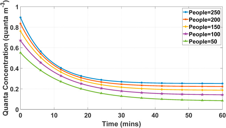
According to Eqs. (7), (8), (9), (10), virus quanta concentration is directly related to the number of already infected people, which is determined by the occupant density in the building. As a result, as the occupant density increases, the virus quanta concentration value would increase, and consequently, infection risk and the number of newly infected people will increase. Fig. 5 shows the number of virus concentration for the university building.
Fig. 5.
Changes in the virus quanta concentration over time with different numbers of occupants for the university building.
This figure shows the exponential relationship between quanta concentration and time. According to this figure, virus particles increase with the occupant density and as time passes, they start to inactivate and settle, and eventually, the existing virus particles in the building incline to a constant value which is determined by the other parameters. Fig. 6 represents the infection risk of occupants depending on the number of occupants in the building and exposure duration.
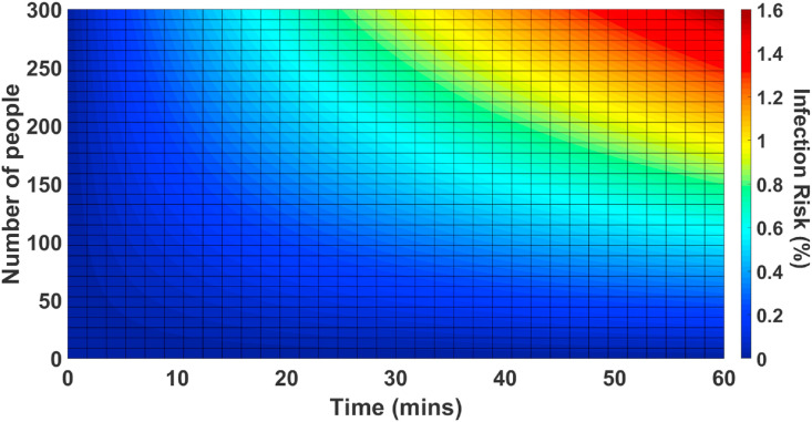
Fig. 6.
The relation between the infection risk with the exposure time and number of present people in the building.
According to this figure, the more exposed the occupants are to others, the greater the risk of infection would be. Furthermore, as the occupant density increases in the building, the risk of infection, and accordingly the number of infected people would increase. According to this figure, staying 15 min in this building exposing to 300 occupants has the same infection risk as staying 60 min exposed to 100 people.
4. Result and discussion
4.1. Validation
EnergyPlus is utilized for the energy simulation of this problem. Therefore, the equations and parameters of this model for the energy analysis are pre-defined in EnergyPlus. Many validations for this software have been presented in various studies [[70], [71], [72]] which validates the results of this software in building energy simulations.
For COVID-19 virus infection risk, the number of infected people with the virus depends on a large number of indeterminate parameters that cannot be measured easily, which makes it difficult to accurately model this phenomenon. Moreover, there are many complex ways of virus transmission between people, but in this article, only the respiratory transmission risk is studied. In order to validate the mathematical model for estimating the number of infected people with the virus, data from several universities in the United States have been used as the validation references, which are gathered in Table 6 [73].
Table 6.
Virus transmission model's validation data.
| University Name | Total Students | Closing Date | Reported Infections | Modeled Infections |
|---|---|---|---|---|
| University of Berkeley | 31348 | 10 March, 2020 | 123 | 115.22 |
| University of Washington | 32000 | 20 March, 2020 | 249 | 220.56 |
| Central Michigan University | 19431 | 11 March, 2020 | 16 | 8.77 |
| Stanford University | 17249 | 10 March, 2020 | 99 | 71.51 |
Infections that are reported by the universities, happen through various transmission mechanisms. Since the studied mathematical model only takes into account infection through droplets, the reported infections in the universities need to be limited to this mechanism for the sake of validation. It is reported that about 78–85% of COVID-19 infections happen through droplets and close contacts with infected cases [74]. Therefore, by considering only the reported infections that have happened through droplets, the accuracy of the model varies from 70% for the Central Michigan University to a maximum of 96% for the University of Washington. The resulted errors are mainly systematic errors (bias), which are originated from the inherent uncertainties (e.g. ignoring the facial masks, not having access to the actual presence pattern of students, ignoring the immune systems of occupants, etc.) [75,76]. Since no validations have been performed in this context before, there is no pre-specified acceptable range of accuracy for this validation. However, accuracy of the model in most of the cases is within the accepted accuracy range of some other related research models [77,78]. Therefore, the results successfully confirm the mathematical model.
4.2. Cold season
As a representative period for cold weather conditions, the range of January 1st to January 5th of 2020 has been chosen for the simulations. Fig. 7 shows the climatic conditions of the region in the mentioned period. It is concluded from Fig. 7.a that the HVAC systems have been able to adjust the PMV value to a constant number of 0 during work hours in variable climate conditions and therefore, it confirms the functionality of these systems.
Fig. 7.
(a) PMV value during the period of simulation and the ambient and building temperatures. (b) Wind speed and solar radiation levels for the case study during the winter days.
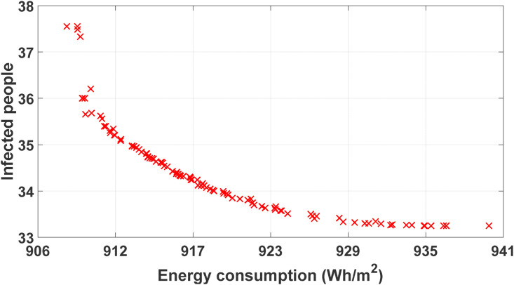
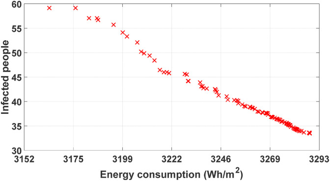
The result of this optimization problem would be a set of non-dominated chromosomes that form a Pareto front. This set of solutions provide a collection of the best possible solutions for the problem. The resulted Pareto front for the abovementioned period is shown in Fig. 8 . According to this figure, the minimum number of infected people is 33.25 and the minimum energy consumption has resulted as 907.7 Wh/m2 within 5 days.
Fig. 8.
Set of possible solutions for the optimization problem in winter days.
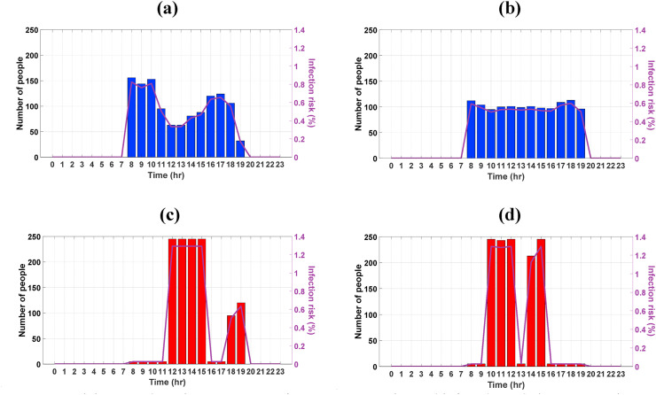
To make a comparison between the best and worst scenarios in terms of both energy consumption and infected people, a reverse optimization operation was performed which maximizes the objective functions. The obtained results of the best and worst occupant distributions in this building, based on the energy consumption and the infected people with the virus are given in Fig. 9 .
Fig. 9.
Minimum and maximum amounts of energy consumption and infected people in 5 consecutive days in winter. (a) Case with the lowest energy consumption of 907.7 Wh/m2. (b) Case with the lowest infected people of 33.24. (c) Case with the highest energy consumption of 1332.3 Wh/m2. (d) Case with the highest infected people of 75.16.
Fig. 9 represents a set of best and worst population distributions during the run period, for both objective functions.
Fig. 9.a is representing a population distribution pattern with the lowest energy consumption in the building, which is 907.7 Wh/m2. According to this figure, a slight depression in the bars has happened at noon and about 150 occupants are present in the opening hours. This pattern can be utilized in buildings to consume the lowest amount of heating energy in the buildings. In this scenario, the maximum number of present occupants in a particular time is 150, meaning that no more than about 7.5 classes per hour should be held during these days to achieve the lowest amount of energy consumption.
Fig. 9.b represents a pattern with the lowest infected people counts. The population distribution in the building within a day is almost uniform with an average amount of about 100 people. This is resulted in forming 5 classes per hour within these days. The total amount of infected people by this optimum pattern through 5 winter days is 33.24 people.
Fig. 9.c shows the case with the highest energy consumption within this period. According to this figure, the population distribution is non-uniform and in some particular times of the day it reaches up to the maximum number of 245 occupants, while in some other hours it has the minimum number of 5 people. By comparing this figure with Fig. 9.a, it is observed that the occupant distribution patterns of these cases are opposite. The consumed amount of energy in this pattern is 1332.3 Wh/m2, which is 47% more than the optimal model, shown in Fig. 9.a.
Eventually, Fig. 9.d shows a pattern with the highest number of infected people. According to this figure, at certain times of the day, the number of occupants in the building are 245 and at the other certain hours, it is the minimum amount of 5, forming an extremely uneven population distribution. In this case, 75.16 people are infected with the virus within 5 days, which is 126% more than the optimal scenario of Fig. 9.b. This population distribution occurs when all the classes are simultaneously formed at certain hours of the day while no classes are formed at some other hours of the day, which as a result, drastically increases the number of infected people. Therefore, the occupant distribution in a building in winter has a major impact on the number of infected people and the energy consumption in the building.
4.3. Hot season
As a representative period for hot days, the range of July 1st to July 5th of 2020 has been considered for simulations. The parameters of the simulation are the same as the cold seasons. Fig. 10 shows the climatic conditions of the region in the considered periods. From Fig. 10.a it can be concluded that the cooling systems have been able to fix the PMV value to 0 as well, just like Fig. 8.
Fig. 10.
a) PMV values during the period of simulation and the ambient and building temperatures. (b) Wind speed and solar radiation levels for the case study during the summer days.
The set of optimum solutions for this optimization problem, forming a Pareto front, is shown in Fig. 11 . According to this figure, the case with the minimum number of infected people has 33.46 infected people and the case with the minimum amount of energy consumption has 3163.7 Wh/m2 energy consumption.
Fig. 11.
Set of possible solutions for the optimization problem in summer days.
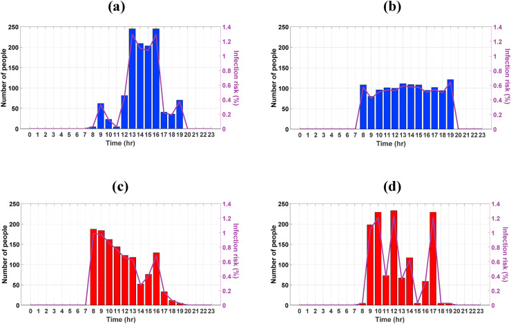
Just like the winter case, discussed in section 4.3, a maximization problem is solved to identify the worst population distribution pattern and compare the results with the optimum ones. Fig. 12 represents the best and worst occupant presence pattern in the building in terms of energy consumption and the number of infected people.
Fig. 12.
Minimum and maximum amounts of energy consumption and infected people in 5 consecutive days in summer. (a) Case with the lowest energy consumption of 3163.7 Wh/m2. (b) Case with the lowest infected people of 33.46. (c) Case with the highest energy consumption of 3311.6 Wh/m2. (d) Case with the highest infected people of 59.58.
Fig. 12.a belongs to the case with the lowest energy consumption. In this model, the population distribution is not uniform and varies between the maximum and minimum count of 245 and 5 within a day, which results in the minimum energy consumption of 3163.7 Wh/m2 for 5 days. According to the figure, the occupant distribution is aligned with the climatic conditions.
Fig. 12.b shows the population distribution pattern with the lowest number of infected people with the virus in summer days, which is 33.46 people within 5 days. According to this figure, the distribution of occupants within the working hours is almost uniform, with an average amount of 100 people, which is a result of forming 5 simultaneous classes per hour in the building, almost the same as Fig. 9.b.
Fig. 12.c represents the highest energy consumption in the building through the run period. This pattern leads to consumes 3312.67 Wh/m2 energy, which is 5% more energy than the case with the least energy consumption (Fig. 12.a). Therefore, it can be concluded that the occupant distribution doesn't tend to have a strong impact on the building's energy consumption in the summer days, unlike the winter days.
Fig. 12.d shows the occupant presence pattern with the highest infected people with COVID-19 virus. This pattern results in 59.58 infected people in summer, which is 78% more than the optimum pattern obtained from Fig. 12.b. Therefore, the occupant distribution in this building within the summer days, has a major effect on the number of infected people, while having a slight impact on the overall energy consumption.
4.4. Sensitivity analysis
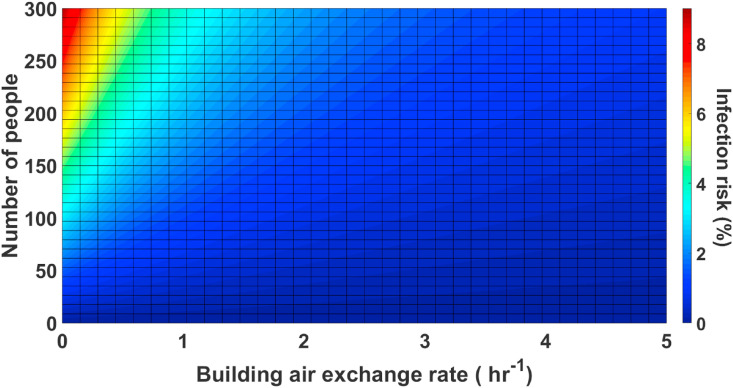
As shown in Eqs. (7), (9), there are many parameters for specifying the infected people numbers and also the building energy consumption. Among these affecting parameters, the air exchange rate is one of the most important factors, determining the energy consumption and the number of infected people with the virus. According to Fig. 4, it is clear that in winter, the outdoor air temperature is less than the desired temperature in the room so that heating coils will require much more energy to adjust the room's temperature. In the same way, in summer the outdoor air temperature is higher than the adjusted temperature in the thermal zones and as a result, the cooling coils would require more energy to be able to retain the zone's temperature in desirable conditions. So almost at any time of the year, increasing the fresh air flowrate would result in higher HVAC energy consumption in the building. The results obtained by Guo's study also confirms this fact [32]. On the other hand, according to Eqs. (7), (8), (9), (10), an increase in the outside air flowrate would result in more virus elimination rate () in the zone and accordingly fewer existing virus particles in the room. Therefore, the risk of infection would decrease exponentially, and the number of infected people would fall. So, assuming that the other parameters of the virus transmission equation are constant, the time of the year wouldn't affect this relationship and an increase in the fresh air flowrate would result in more virus elimination rate and will decrease the number of infected people with the same amount. Fig. 13 shows the relationship between the occupant count and air exchange rate with the COVID-19 infection risk in the building.
Fig. 13.
The relationship between the number of people and building air exchange rate with the COVID-19 infection risk.
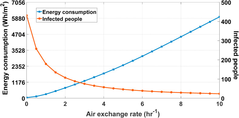
To understand the effect of the air exchange rate and ventilation of the building on the energy consumption and the number of infected people, many air exchange rate values were considered for the building and the objective functions were evaluated for each. Fig. 14 represents the results of this analysis. According to this figure, as the air exchange rate increases, the number of infected people with the virus decreases exponentially, but the building energy consumption also increases. Air exchange rate value of 2.8 hr−1 is obtained as the optimum value where two objective functions meet and can be introduced as the balance point for the building.
Fig. 14.
The relationship between the air exchange rate with the energy HVAC energy consumption and the number of infected people with COVID-19 in the building.
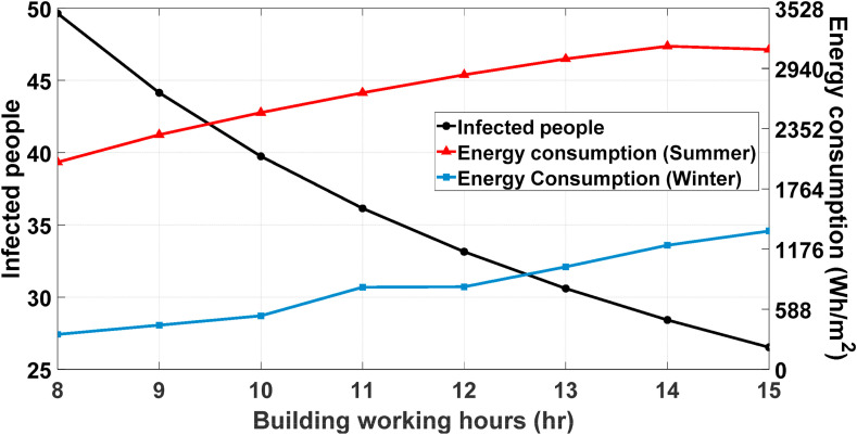
As another important parameter in determining the energy consumption and the number of infected people with COVID-19, the working hours of the university were further studied and analyzed. Extending the working hours of buildings means increasing the times that occupants are present in the building and therefore, HVAC systems need to operate longer. With any extension in the working hours of the building, despite having less dense occupant distribution within the day, HVAC systems would require more energy to provide the desired thermal conditions for the occupants in these hours. So, extending the working hours of the building results in extra energy consumption in HVAC systems that varies by the temperature difference of the indoors and outdoors. As discussed earlier, extending the working hours of a building leads to a less occupant density within a day. According to Eqs. (7), (8), (9), (10), less occupant density in a building comes with a lower number of already infected people () in the building. In consequence, this will decrease the virus particles in the building and so fewer people would be infected with the virus. Therefore, assuming that other parameters of virus transmission remain constant, any extent in the working hours of the buildings results in a lower number of infected people. In this regard, a uniform population distribution within a day was considered, and by changing the working hours of the university and the building, energy consumptions and the number of infected people were examined. Accordingly, the starting hour of the building is considered to be 6 a.m. and the closing hours vary from 2 p.m. to 9 p.m. The results of this investigation are shown in Fig. 15 . According to this figure, as the number of working hours of the building increases, the population density decreases and so the number of infected people decreases as well, but the HVAC energy consumption rises. Moreover, it is concluded that increasing the working hours of the building from 12 to 13 h, decreases the number of infected people by 7.67% and in contrast, energy consumption in winter and summer increased by 24.11% and 5.4%, respectively.
Fig. 15.
Changes in HVAC energy consumption and the number of infected people with COVID-19 in the building with different building working hours in winter and summer.
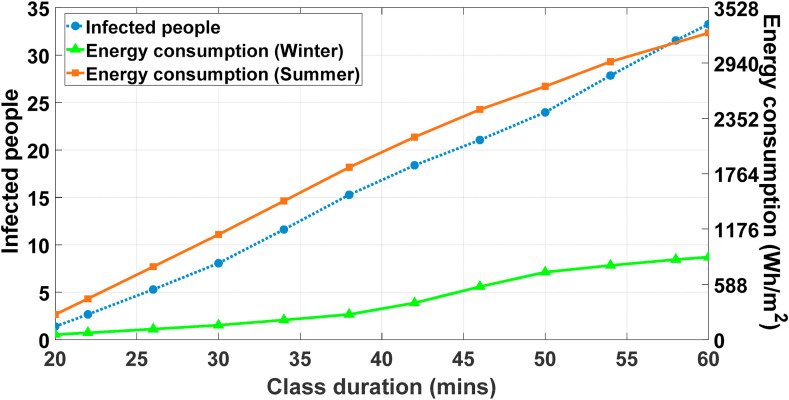
As another essential parameter affecting the number of infected people with COVID-19 and energy consumption, class duration time is examined. The class duration time is denoted as the exposure time () in Eq. (9), which has a direct relationship with virus infection risk and also with energy consumption. In the previous simulations, class durations were considered to be 1 h. In both winter and summer, any extension in the class duration means that HVAC systems need to work longer to provide thermal comfort for the occupants. So, it can be concluded that when a part of class time is dedicated to virtual learning to decrease the class duration, it is expected to have less energy consumption in the building. On the other hand, as the class duration is extended, the exposure time for the present occupants () increases. According to Eq. (7) and Fig. 5, virus quanta concentration in the building is indirectly related to the time. So, as time passes, virus particles start to settle and deactivate and finally harmonize by the exhalation rate of the infected people and the air exchange rate. But on the other hand, Eq. (9) proves that longer exposure in a space with infected people increases the risk of infection. In general, it turns out that shortening the class duration results in a lower number of infected people.
For further investigating the impact of class duration on the objective functions, the population distribution of the lowest infected people case in winter is selected as a study case. Fig. 16 represents the results of this examination. According to Fig. 16, it can be seen that reducing the class duration from 60 min to 40 min results in a reduction of 49.6% in the number of infected people with COVID-19 and respectively 28% and 28.6% in energy consumption in winter and summer. Eventually, it can be concluded that reducing the class duration by allocating a part of it to virtual education, can have a significant impact on reducing the number of infected people and also energy consumption.
Fig. 16.
Variation of infected people with COVID-19 and the HVAC energy consumption with class durations for winter and summer.
5. Conclusion
The purpose of this study was to investigate the impacts of the presence of occupants, air exchange rate, class duration, and working hours of a university building on the HVAC system's energy consumptions and the number of infected people with COVID-19 in buildings. Many parameters affecting COVID-19 infection risk and energy consumption exist in buildings, and in this paper, the four most dominant parameters that were more controllable and also their information were accessible, were chosen to study their effects on the objective functions. However, the results of this study show a strong relationship between these parameters and the objective functions.
Most of the COVID-19 infections happen in public places, so by changing the occupant distribution pattern in these places, it was concluded that a uniform population distribution pattern can reduce the number of infected people by up to 56%. On the other hand, the most optimal population distribution in terms of energy consumption is one that varies by the climatic conditions, which can reduce energy consumption by up to 32%. Additionally, it was concluded that with increasing the ventilation rate in buildings, the number of infected people greatly falls, but conversely, the HVAC system's energy consumption increases. Another examined important parameter is the working hours of the building. It was seen that extending the working hours of the university can reduce the number of infected people and shorter working hours in buildings can reduce the energy consumption in buildings. Furthermore, it was observed that as the class duration decreases, the number of infected people and the HVAC energy consumption in the buildings decrease as well.
Eventually, it can be concluded that during the global pandemic of COVID-19 or any other respiratory viruses, increasing the ventilation rate in the building as much as possible, reducing the class durations, and increasing the working hours of the university, can greatly reduce the number of infected people with the virus. Moreover, Virtual learning can be applied fully or along with in-person classes, which would reduce student attendance on campus. On the other hand, in non-epidemic conditions, by reducing the ventilation rate in the building, shortening the class durations and the working hours of the university, it is possible to save a significant amount of energy in the buildings. Therefore, by choosing the right approach with a proper tradeoff, it is possible to minimize the number of infected people by any virus and the HVAC energy consumption in buildings.
Accordingly, towards eradicating the COVID-19 and any other respiratory viruses, governments should particularly focus on public places and enforce new rules. In this regard, all buildings are recommended to maximize the ventilation rate to reduce the infection risk and decrease the ventilation rate up to the allowed rate to consume less energy. Buildings that can schedule occupant's presence (e.g. universities, clinics, beauty salons, etc.) can utilize a uniform population distribution pattern to significantly reduce the infection risk of COVID-19 and other respiratory viruses and utilize a climate-adaptive population distribution pattern to decrease the energy consumption. Buildings that have multiple attendees in a day (e.g. universities, malls, stores, clinics, etc.) can extend the working hours and shorten the presence time of occupants to minimize the infection risk and can decrease the working hours to consume less energy.
Declaration of competing interest
The authors declare that they have no known competing financial interests or personal relationships that could have appeared to influence the work reported in this paper.
References
- 1.Fesanghary M., Asadi S., Geem Z.W. Design of low-emission and energy-efficient residential buildings using a multi-objective optimization algorithm. Build. Environ. 2012;49:245–250. [Google Scholar]
- 2.International Energy Outlook. EIA; 2018. Accessed on. 2018. [Google Scholar]
- 3.Wang C., et al. Dynamic occupant density models of commercial buildings for urban energy simulation. Build. Environ. 2020;169:106549. [Google Scholar]
- 4.Hu S., et al. Building and Environment; 2020. A Systematic Review of Occupant Behavior in Building Energy Policy; p. 106807. [Google Scholar]
- 5.Salim F.D., et al. Building and Environment; 2020. Modelling Urban-Scale Occupant Behaviour, Mobility, and Energy in Buildings: A Survey; p. 106964. [Google Scholar]
- 6.Bai Y., et al. Presumed asymptomatic carrier transmission of COVID-19. Jama. 2020;323(14):1406–1407. doi: 10.1001/jama.2020.2565. [DOI] [PMC free article] [PubMed] [Google Scholar]
- 7.Abdel-Basset M., Abdel-Fatah L., Sangaiah A.K. Computational Intelligence for Multimedia Big Data on the Cloud with Engineering Applications. Elsevier; 2018. Metaheuristic algorithms: a comprehensive review; pp. 185–231. [Google Scholar]
- 8.Deb K., et al. A fast and elitist multiobjective genetic algorithm: NSGA-II. IEEE Trans. Evol. Comput. 2002;6(2):182–197. [Google Scholar]
- 9.Eberhart R., Kennedy J. MHS'95. Proceedings of the Sixth International Symposium on Micro Machine and Human Science. Ieee; 1995. A new optimizer using particle swarm theory. [Google Scholar]
- 10.Zitzler E., Laumanns M., Thiele L. TIK-report; 2001. SPEA2: Improving the Strength Pareto Evolutionary Algorithm; p. 103. [Google Scholar]
- 11.Carlucci S., et al. Multi-objective optimization of a nearly zero-energy building based on thermal and visual discomfort minimization using a non-dominated sorting genetic algorithm (NSGA-II) Energy Build. 2015;104:378–394. [Google Scholar]
- 12.Delgarm N., et al. A novel approach for the simulation-based optimization of the buildings energy consumption using NSGA-II: case study in Iran. Energy Build. 2016;127:552–560. [Google Scholar]
- 13.Zhou Y., et al. Multi-objective optimisation of an interactive buildings-vehicles energy sharing network with high energy flexibility using the Pareto archive NSGA-II algorithm. Energy Convers. Manag. 2020;218:113017. [Google Scholar]
- 14.Nguyen A.-T., Reiter S., Rigo P. A review on simulation-based optimization methods applied to building performance analysis. Appl. Energy. 2014;113:1043–1058. [Google Scholar]
- 15.Naderi E., et al. Multi-objective simulation-based optimization of controlled blind specifications to reduce energy consumption, and thermal and visual discomfort: case studies in Iran. Build. Environ. 2020;169:106570. [Google Scholar]
- 16.Huovila A., Tyni A., Dooley K. SB13 Dubai Conference. 2013. Building occupancy as an aspect of energy efficiency. [Google Scholar]
- 17.Menezes A.C., et al. Predicted vs. actual energy performance of non-domestic buildings: using post-occupancy evaluation data to reduce the performance gap. Appl. Energy. 2012;97:355–364. [Google Scholar]
- 18.Dedesko S., et al. Methods to assess human occupancy and occupant activity in hospital patient rooms. Build. Environ. 2015;90:136–145. [Google Scholar]
- 19.Ryu S.H., Moon H.J. Development of an occupancy prediction model using indoor environmental data based on machine learning techniques. Build. Environ. 2016;107:1–9. [Google Scholar]
- 20.Kang H., et al. Determining the optimal occupancy density for reducing the energy consumption of public office buildings: a statistical approach. Build. Environ. 2018;127:173–186. [Google Scholar]
- 21.Li X., Yao R. A machine-learning-based approach to predict residential annual space heating and cooling loads considering occupant behaviour. Energy. 2020;212:118676. [Google Scholar]
- 22.Wang Z., Hong T., Piette M.A. Predicting plug loads with occupant count data through a deep learning approach. Energy. 2019;181:29–42. [Google Scholar]
- 23.Sun Y., et al. Data-driven occupant-behavior analytics for residential buildings. Energy. 2020;206:118100. [Google Scholar]
- 24.Jami, S., et al., The effect of occupant behaviors on energy retrofit: a case study of student dormitories in Tehran. J. Clean. Prod. 278: p. 123556.
- 25.Wood R., et al. Quantification of shared air: a social and environmental determinant of airborne disease transmission. PloS One. 2014;9(9) doi: 10.1371/journal.pone.0106622. [DOI] [PMC free article] [PubMed] [Google Scholar]
- 26.Andrews J.R., et al. Integrating social contact and environmental data in evaluating tuberculosis transmission in a South African township. J. Infect. Dis. 2014;210(4):597–603. doi: 10.1093/infdis/jiu138. [DOI] [PMC free article] [PubMed] [Google Scholar]
- 27.Horve P.F., et al. Building upon current knowledge and techniques of indoor microbiology to construct the next era of theory into microorganisms, health, and the built environment. J. Expo. Sci. Environ. Epidemiol. 2019:1–17. doi: 10.1038/s41370-019-0157-y. [DOI] [PMC free article] [PubMed] [Google Scholar]
- 28.Saari A., et al. The effect of a redesigned floor plan, occupant density and the quality of indoor climate on the cost of space, productivity and sick leave in an office building–A case study. Build. Environ. 2006;41(12):1961–1972. [Google Scholar]
- 29.Kovesi T., et al. Indoor air quality and the risk of lower respiratory tract infections in young Canadian Inuit children. CMAJ (Can. Med. Assoc. J.) 2007;177(2):155–160. doi: 10.1503/cmaj.061574. [DOI] [PMC free article] [PubMed] [Google Scholar]
- 30.Zhan J., et al. Environmental impacts on the transmission and evolution of COVID-19 combing the knowledge of pathogenic respiratory coronaviruses. Environ. Pollut. 2020:115621. doi: 10.1016/j.envpol.2020.115621. [DOI] [PMC free article] [PubMed] [Google Scholar]
- 31.Ronchi E., Lovreglio R. 2020. EXPOSED: an Occupant Exposure Model for Confined Spaces to Retrofit Crowd Models during a Pandemic. arXiv preprint arXiv:2005.04007. [DOI] [PMC free article] [PubMed] [Google Scholar]
- 32.Guo M., et al. Building and Environment; 2020. Review and Comparison of HVAC Operation Guidelines in Different Countries during the COVID-19 Pandemic; p. 107368. [DOI] [PMC free article] [PubMed] [Google Scholar]
- 33.Wee L.E.I., et al. Containing COVID-19 outside the isolation ward: the impact of an infection control bundle on environmental contamination and transmission in a cohorted general ward. Am. J. Infect. Contr. 2020;48(9):1056–1061. doi: 10.1016/j.ajic.2020.06.188. [DOI] [PMC free article] [PubMed] [Google Scholar]
- 34.Rahman H.S., et al. Masrur Sleman Aziz, Ridha Hassan Hussein, Hemn Hassan Othman, Shirwan Hama Salih Omer, Eman Star Khalid, Nusayba Abdulrazaq Abdulrahman, Kawa Amin, Rasedee Abdullahg, The transmission modes and sources of COVID-19: a systematic review. International Journal of Surgery Open. 2020;26:125–136. doi: 10.1016/j.ijso.2020.08.017. [DOI] [PMC free article] [PubMed] [Google Scholar]
- 35.Sun C., Zhai Z. The efficacy of social distance and ventilation effectiveness in preventing COVID-19 transmission. Sustain. Cities Soc. 2020;62:102390. doi: 10.1016/j.scs.2020.102390. [DOI] [PMC free article] [PubMed] [Google Scholar]
- 36.McCollum D.L., et al. Energy modellers should explore extremes more systematically in scenarios. Nat. Energy. 2020;5(2):104–107. [Google Scholar]
- 37.Crawley D.B., et al. Energy plus: energy simulation program. ASHRAE J. 2000;42(4):49–56. [Google Scholar]
- 38.Zhang Q., Li H. MOEA/D: a multiobjective evolutionary algorithm based on decomposition. IEEE Trans. Evol. Comput. 2007;11(6):712–731. [Google Scholar]
- 39.Deb K., Jain H. An evolutionary many-objective optimization algorithm using reference-point-based nondominated sorting approach, part I: solving problems with box constraints. IEEE Trans. Evol. Comput. 2013;18(4):577–601. [Google Scholar]
- 40.DoE U. 2010. Energyplus Engineering Reference. The Reference to Energyplus Calculations. [Google Scholar]
- 41.Standard A. vol. 3. 2004. (ASHRAE 55-2004. Thermal Environmental Conditions for Human Occupancy). [Google Scholar]
- 42.Dostal J., Baumelt T. E3S Web of Conferences. EDP Sciences; 2019. Model predictive control for buildings with active one-pipe hydronic heating. [Google Scholar]
- 43.Fanger P.O. 1970. Thermal Comfort. Analysis and Applications in Environmental Engineering. Thermal Comfort. Analysis and Applications in Environmental Engineering. [Google Scholar]
- 44.ISO I. 7730: ergonomics of the thermal environment—analytical determination and interpretation of thermal comfort using calculation of the PMV and PPD indices and local thermal comfort criteria. Management. 2005;3(605):e615. [Google Scholar]
- 45.Riley E., Murphy G., Riley R. Airborne spread of measles in a suburban elementary school. Am. J. Epidemiol. 1978;107(5):421–432. doi: 10.1093/oxfordjournals.aje.a112560. [DOI] [PubMed] [Google Scholar]
- 46.Gammaitoni L., Nucci M.C. Using a mathematical model to evaluate the efficacy of TB control measures. Emerg. Infect. Dis. 1997;3(3):335. doi: 10.3201/eid0303.970310. [DOI] [PMC free article] [PubMed] [Google Scholar]
- 47.Buonanno G., Stabile L., Morawska L. Environment International; 2020. Estimation of Airborne Viral Emission: Quanta Emission Rate of SARS-CoV-2 for Infection Risk Assessment; p. 105794. [DOI] [PMC free article] [PubMed] [Google Scholar]
- 48.Wagner B.G., Coburn B.J., Blower S. Calculating the potential for within-flight transmission of influenza A (H1N1) BMC Med. 2009;7(1):81. doi: 10.1186/1741-7015-7-81. [DOI] [PMC free article] [PubMed] [Google Scholar]
- 49.Knibbs L.D., et al. Room ventilation and the risk of airborne infection transmission in 3 health care settings within a large teaching hospital. Am. J. Infect. Contr. 2011;39(10):866–872. doi: 10.1016/j.ajic.2011.02.014. [DOI] [PMC free article] [PubMed] [Google Scholar]
- 50.Yang W., Marr L.C. Dynamics of airborne influenza A viruses indoors and dependence on humidity. PloS One. 2011;6(6) doi: 10.1371/journal.pone.0021481. [DOI] [PMC free article] [PubMed] [Google Scholar]
- 51.Stephens B. National Air Filtration Association (NAFA) Foundation Report; 2012. HVAC filtration and the Wells-Riley approach to assessing risks of infectious airborne diseases. [Google Scholar]
- 52.Climate of Tehran. 2010. [Google Scholar]
- 53.Malik W.S. The International Educator; 2015. Planning a New School. [Google Scholar]
- 54.ASHRAE . 2005. ASHRAE 2005 HOF Materials. [Google Scholar]
- 55.Standard A. ASHRAE; Atlanta, GA: 2013. Standard 62.2-2013,“. Ventilation for Acceptable Indoor Air Quality in Low-Rise Residential Buildings. [Google Scholar]
- 56.U.S. General Services Administration https://www.gsa.gov/ Available from:
- 57.team W. 2020. Coronavirus Disease (COVID-19): Ventilation and Air Conditioning in Public Spaces and Buildings.https://www.who.int/news-room/q-a-detail/coronavirus-disease-covid-19-ventilation-and-air-conditioning-in-public-spaces-and-buildings Available from: [Google Scholar]
- 58.Covid-19 Pandemic Statistics. 2020. https://www.worldometers.info/coronavirus/ Available from: [Google Scholar]
- 59.reportCoronavirus Disease 2019 (COVID-19) Situation Report.
- 60.Rudnick S., Milton D. Risk of indoor airborne infection transmission estimated from carbon dioxide concentration. Indoor Air. 2003;13(3):237–245. doi: 10.1034/j.1600-0668.2003.00189.x. [DOI] [PubMed] [Google Scholar]
- 61.Liao C.M., Chang C.F., Liang H.M. A probabilistic transmission dynamic model to assess indoor airborne infection risks. Risk Anal.: Int. J. 2005;25(5):1097–1107. doi: 10.1111/j.1539-6924.2005.00663.x. [DOI] [PubMed] [Google Scholar]
- 62.Beggs C.B., Shepherd S.J., Kerr K.G. Potential for airborne transmission of infection in the waiting areas of healthcare premises: stochastic analysis using a Monte Carlo model. BMC Infect. Dis. 2010;10(1):247. doi: 10.1186/1471-2334-10-247. [DOI] [PMC free article] [PubMed] [Google Scholar]
- 63.Sze To G.N., Chao C.Y.H. Review and comparison between the Wells–Riley and dose‐response approaches to risk assessment of infectious respiratory diseases. Indoor Air. 2010;20(1):2–16. doi: 10.1111/j.1600-0668.2009.00621.x. [DOI] [PMC free article] [PubMed] [Google Scholar]
- 64.Nardell E.A., et al. Airborne infection. Theoretical limits of protection achievable by building ventilation. Am. Rev. Respir. Dis. 1991;144:302–306. doi: 10.1164/ajrccm/144.2.302. [DOI] [PubMed] [Google Scholar]
- 65.Escombe A.R., et al. Natural ventilation for the prevention of airborne contagion. PLoS Med. 2007;4(2):e68. doi: 10.1371/journal.pmed.0040068. [DOI] [PMC free article] [PubMed] [Google Scholar]
- 66.Chen S.C., et al. A probabilistic transmission model to assess infection risk from Mycobacterium tuberculosis in commercial passenger trains. Risk Anal.: Int. J. 2011;31(6):930–939. doi: 10.1111/j.1539-6924.2010.01552.x. [DOI] [PubMed] [Google Scholar]
- 67.Qian H., et al. Spatial distribution of infection risk of SARS transmission in a hospital ward. Build. Environ. 2009;44(8):1651–1658. [Google Scholar]
- 68.Chatoutsidou S.E., Lazaridis M. Assessment of the impact of particulate dry deposition on soiling of indoor cultural heritage objects found in churches and museums/libraries. J. Cult. Herit. 2019;39:221–228. [Google Scholar]
- 69.Van Doremalen N., et al. Aerosol and surface stability of SARS-CoV-2 as compared with SARS-CoV-1. N. Engl. J. Med. 2020;382(16):1564–1567. doi: 10.1056/NEJMc2004973. [DOI] [PMC free article] [PubMed] [Google Scholar]
- 70.Shrestha S., Maxwell G. Proceedings of Building Simulation. 2011. Empirical validation of building energy simulation software: EnergyPlus. [Google Scholar]
- 71.Zhu D., et al. Building Simulation. Springer; 2013. A detailed loads comparison of three building energy modeling programs: EnergyPlus, DeST and DOE-2.1 E. [Google Scholar]
- 72.Sullivan R. Final Report; 1998. Validation studies of the DOE-2 building energy simulation program. [Google Scholar]
- 73.Weiyi Cai D.I. The Newyork Times. 2020. Mitch smith, alex lemonides and lauryn higgins, more than 6,600 coronavirus cases have been linked to U.S. Colleges. [Google Scholar]
- 74.Organization W.H. World Health Organization; 2020. Transmission of SARS-CoV-2: Implications for Infection Prevention Precautions: Scientific Brief. 09 July 2020. [Google Scholar]
- 75.Sargent R.G. Verification and validation of simulation models. J. Simulat. 2013;7(1):12–24. [Google Scholar]
- 76.Thacker B.H., et al. Los Alamos National Lab; 2004. Concepts of model verification and validation. [Google Scholar]
- 77.Mahajan A., Sivadas N.A., Solanki R. An epidemic model SIPHERD and its application for prediction of the spread of COVID-19 infection in India. Chaos, Solit. Fractals. 2020;140:110156. doi: 10.1016/j.chaos.2020.110156. [DOI] [PMC free article] [PubMed] [Google Scholar]
- 78.Barda N., et al. Developing a COVID-19 mortality risk prediction model when individual-level data are not available. Nat. Commun. 2020;11(1):1–9. doi: 10.1038/s41467-020-18297-9. [DOI] [PMC free article] [PubMed] [Google Scholar]


