Abstract
In this paper, Transfer Learning is used in LSTM networks to forecast new COVID cases and deaths. Models trained in data from early COVID infected countries like Italy and the United States are used to forecast the spread in other countries. Single and multistep forecasting is performed from these models. The results from these models are tested with data from Germany, France, Brazil, India, and Nepal to check the validity of the method. The obtained forecasts are promising and can be helpful for policymakers coping with the threats of COVID-19.
Keywords: COVID-19, Long Short Term Memory (LSTM), Time-series-forecast, Transfer Learning, Neural network
1. Introduction
COVID-19 was first detected in Wuhan City in December 2019. Since then it has caused more than seven hundred thousand deaths and twenty million infections [1]. With such massive scale fatalities, it has become one of the greatest crises of this generation. Apart from the loss of human lives, the pandemic has caused serious damage to the world economy. Because of lockdowns and similar distancing strategies it has also adversely affected psychological and social sections [2].
In the absence of any proven medicine or vaccine at present, an intervention strategy may be more useful to control the spread [3]. An effective modeling method to forecast the spread of the virus among the population can be extremely useful to prepare and formulate health and economic policies for any government or administrators. From planning emergency hospitals, managing ventilators, and medical resources to regulating lock-downs and scheduling economic activities, effective forecasts are strategically very important for policymakers [4]. When new cases rise at a rate of thousands per day then even the most developed nation’s healthcare system has been overwhelmed to handle a large number of patients. A timely forecast can prepare the responsible authority accordingly to manage efficiently even during overwhelming scenarios.
With the rise of cases and the availability of more data, various studies [5], [6], [7] have presented mathematical models for the spread. However, most of the models have a limited scope of forecasts for a particular country or region only. Previous researches [8], [9] have also used LSTM models to forecast but they use old data of the same country which is pretty limited. As it may not have seen and learned from the various patterns like sharp spikes and flattening effects, the learning process may be incomplete and imprecise. These dynamic patterns are more prevalent in early infected countries like Italy which have now passed the sharp spiking and gradual flattening for new cases. The use of Transfer Learning may help the network to model all these highly non-linear temporal patterns which the test country may have never seen in its history. For countries like France, Italy the earlier occurrence and spread provides a large dataset for training which is not available for countries that saw the spread later like India and Nepal, which imposed strict lockdown early but is easing the regulations now. This discrepancy in pandemic over various regions has provided mature data for earlier infected countries.
Cluster analysis [10] study has shown similarities existing in the dynamics of the spread of the disease between various countries like Italy, France, and Germany which has similar intervention modalities. Though there may be some level of similarity in intervention techniques and timing, even then the countries can have massive differences in scale of spread and mortality rate. These differences are very prominent across countries in the European Union. A generalized forecasting model incorporating a wider region is thus a difficult challenge owing to all the differences existing across nations.
The paper implements Transfer Learning to LSTM models which learn separately from the data of Italy and the United States. It then applies these trained models i.e. the architecture along with weights, to forecast new COVID cases and deaths. The results are tested for France, Germany, Brazil, India, and Nepal. For both the models, separate networks have been trained to forecast for one and five days.
2. Material and methods
2.1. Dataset
The data has been obtained from an open dataset of Our World in Data [11] which maintains and updates global data daily acquired from the European Center for Disease Prevention and Control (ECDC). The data was available from the 31st of December to the 10th of June. However, the data from February 28th onwards has been used for training purpose during which cases were more active. Data for the number of new cases per 100 thousand of the population per day is one of the forecasting variables.
| (1) |
New death cases per million of the populations calculated as in Eq. (2) has also been forecasted from the available data.
| (2) |
Data from 7 countries: Italy, France, Germany, United States, Brazil, India, and Nepal has been used for this study. These test countries cover up 4 continents representing high diversity in intervention techniques, government policies, healthcare system, population density, and levels of spread and death because of COVID-19.
2.2. Moving-average
The data of new cases and new deaths consist of lots of sharp spikes, the noisy data is smoothened using moving average. Moving average can provide more stable data points suitable for the modeling.
Moving average is defined mathematically as:
| (3) |
where,
The study uses a moving average of 3 days for both new cases and new deaths. The reason for using low valued moving average is to smooth out very sharp spikes without changing the actual pattern of the data.
2.3. LSTM network
Recurrent Neural Network (RNN) is one of the most popular and effective deep learning techniques for time series forecasts, because of its ability to memorize sequential information [12]. However, the problems of exploding and vanishing gradient are more common in simple RNN [13]. LSTM solves this problem by introducing a new memory state in RNN [14]. The ability of LSTM networks to capture patterns in data like trends, seasonality, autocorrelations and noise makes it a good candidate for the time series forecast. In a deep neural network, initial layers capture more basic features or patterns and the deeper layer can extract high-level features. As a model trained in one country is used to forecast for the next country, the network should learn basic temporal patterns and avoid memorizing high-level features of a particular dataset. For this single layer LSTM network has been used to avoid any deep and complex architecture. For single and 5-days predictions 1 and 5 units are assigned for this single-layered network. The network does not return any sequences so the output from the LSTM network is the final output. The use of any dense layer has been avoided.
The success of LSTM networks lies in their variety of update, forget, and output gates. Cell state carries the memory of past data and the combination of gates helps the network to determine what information from the past is to be retained and from the present is to be updated. Each cell in the sequence is fed with an activation state () and cell state and the respective input ()
Update gate value (u) is based on the previous activation state () and present input (). Its range is 0 to 1. Weight and bias is learned during training. It provides necessary weightage to the new candidate cell state to determine a new cell state in Eq. (7).
| (4) |
Forget gate value () is also based on previous activation state () and present input (), Weight and bias is updated during training. It is used in the determination of a new cell state in Eq. (8).
| (5) |
Output gate value (o) depends on the previous activation state () and present input (), Weight and bias is updated during the training process. It determines the new activation state by assigning necessary weightage to a new cell state.
| (6) |
New candidate cell state is determined with values of previous activation and present input which will be used to update the new cell state, its influence in the new cell state is determined by the update gate value . The network learns the necessary weights and bias during training.
| (7) |
Cell state () is passed to the next cell with weightage provided by update gate () and forget gate () from Eqs. (4), (5).
| (8) |
New activation () is determined by output gate () and present cell state (). The values of the activation state () and cell state () gets passed to the next cell for repeated operations as explained from Eqs. (4), (5), (6), (7), (8), (9).
| (9) |
is the sigmoid function defined as:
| (10) |
Its output is in the range of 0 to 1. For all the gates i.e. update, forget and output gate the value ranges from 0 to 1, 0 provides no weightage, and 1 represents complete weightage. The output of the hyperbolic tangent (tanh) function ranges from −1 to 1.
The network weights are learned separately from the data of Italy and the United States. During training, these trained weights along with the respective network are then used to forecast for various test countries. Thus, the concept of Transfer Learning enables us to acquire the necessary knowledge from the matured dataset and apply it to forecast for a different country.
2.4. Network architecture
N units of the LSTM network are used where N is the number of days of forecast. As many to one architecture is used, the output of each unit is output to the architecture. So, for 1 and 5 days forecasting 1 and 5 units of LSTM has been assigned in the first layer respectively. The number of cells inside each unit varies according to the window size of the model. Window size refers to the number of past data that is input into the model, this is equal to the number of cells in each LSTM unit. For single-day prediction window size of 8 is chosen i.e. 8 days of past data used as input and the value of 9th-day value is taken as the forecasting value. During training, the network learns respective weights by trying to minimize the error between the actual value on the 9th day and the forecasted value by the network. For 5 days multistep prediction window size of 20 is used i.e. 20 days of past data is input for the network and the consecutive future 5 days data is used as output for the network. The time sequence is maintained both for input and output. A larger window size is used for multistep prediction as more data sequence is necessary to forecast the long-range pattern.
Fig. 1 depicts the architecture for single day prediction, as the window size is eight, the unit has eight cells. Each cell receives sequential input however the output is received from the final cell which is a typical many-to-one architecture. In multistep prediction 5 such sequences as in Fig. 1 are used with 20 cells in each unit. For a particular unit, the weights of trainable parameters across all the cells remain the same. In this architecture, the single-step model has 12 trainable parameters whereas the 5 days prediction model has 140 trainable parameters.
Fig. 1.
Proposed LSTM network for single day prediction.
For training purpose, a batch size of 10 is used. As training data is low in number lower batch size supplies more training batches from available data.
2.5. Network parameters
The LSTM network uses Stochastic Gradient Descent (SGD) optimizer for all of its models with momentum of 0.9. Initially variable learning rate ranging from to is set as a callback function to train along 100 epochs. Then the learning rate corresponding to minimum loss is chosen for actual training of 500 epochs. The same procedure has been used for all the models used in this paper. The details have been tabulated in Table 1.
Table 1.
Network parameters for training.
| Step | Trainable parameters | Batch size | Optimizer | Momentum | Epochs | Learning Rate | Loss Function | Performance metrics |
|---|---|---|---|---|---|---|---|---|
| Singlestep | 12 | 10 | SGD | 0.9 | 500 | 2E−05 | Huber Loss | MAE |
| Multistep | 140 | 10 | SGD | 0.9 | 500 | 1E−05 | Huber loss | MAE |
2.6. Performance parameters
Mean Absolute Error (MAE) and Root Mean Square Error (RMSE) are two metrics used to compare the results from the proposed models.
Mean Absolute Error provides an average absolute error between the forecasted value and real value.
| (11) |
Because of squared error, Root Mean Square Error (RMSE) gives better insights of higher valued error across forecasts.
| (12) |
The normal distribution represents the values of a given distribution as a density of variables. The distribution visualizes the symmetry occurrence in the data around the mean. For multistep prediction, both MAE and RMSE obtained are fitted to normal distribution to see the variation in error across all forecasts. The normal distribution is given by:
| (13) |
where refers to mean and refers to standard deviation.
3. Results and discussion
The paper implements Transfer Learning for the LSTM network to learn from one region and forecast for a completely different region. For training purpose, Keras API with TensorFlow backend [15] is used. Various python libraries have been used for other evaluations. The networks were trained in GPU available in the Google Colab environment [16].
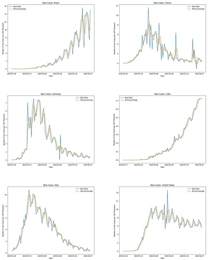
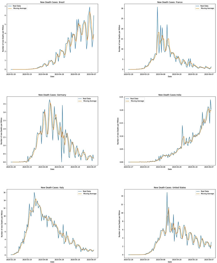
Both the models have been trained and tested in smoothened data whose samples are provided in Fig. 2, Fig. 3. A low value moving average has helped to smooth out sharp spikes without causing any significant distortions to the curves.
Fig. 2.
Samples for data smoothing for new cases.
Fig. 3.
Samples for data smoothing for new death cases.
Two models based on Italy and the United States have been used. Data from December 31st to June 10th was available during modeling. However, the initial part has been truncated when the reported cases and death were limited to single-digit or even 0 in most of the days. For both the models training data ranging from February 28th to June 10th has been taken which encapsulates an active period of the spreading and deaths in these countries. The timeframe for new death cases has been kept consistent with new cases for training as well as testing. It is observed in all datasets, the time series increase or decrease of new cases is consistent with an increase or decrease of new death cases so, the same time frame has been used for death cases as well.
In the United States even as late as February 26th, 0 new cases were recorded but after that, there has been a sharp rise in cases, and during the recorded time frame cases have risen from as low as 1 new case on February 28th to over 30,000 new cases being reported every day during March and April. As for new death cases, the first death in the US was recorded on March 1st and then rose to even 2000 plus new deaths per day within the second week of April. Even by the first week of June, the new death cases were still high approaching 1000 in some cases.
For Italy, new cases reporting surged from the last week of February, until then even as late as February 21st, no new case was reported. During the last week of February, the new death cases were still limited to single-digit however during March and April it reached its peak of over 800 new deaths per day. By the first week of June, the new death cases had decreased to double-digit figures. This time frame thus captures the active period of virus spread and deaths. So, both models start on February 28. During this period, both the countries have reached their peak as of new cases reporting and new death cases.
For testing the models, same timeframe has been used for France, Germany, and Brazil as it represents an active growth time frame for all these countries. However, for India and Nepal COVID spread has got more active lately. This can be explained by strict lockdowns imposed earlier in both countries. For India and Nepal, data from May 2nd to August 11th is used. For all the test countries 102 days have been taken as test days to maintain consistency while comparing results.
3.1. Forecast results
Detailed error calculation for all new cases forecasts has been tabulated in Table 2 and new death cases forecasts have been tabulated in Table 3. The model’s self-forecast i.e. Italy model’s forecast for Italy and the US model’s forecast for the US has not been tabulated for comparison as these are training data for the models.
Table 2.
New cases forecast error.
| 1 Days prediction |
5 Days Prediction |
|||||||||||
|---|---|---|---|---|---|---|---|---|---|---|---|---|
| Target Country | Italy Model |
US Model |
Italy Model |
US Model |
||||||||
| RMSE | MAE | RMSE | MAE | RMSE | RMSE SD | MAE | MAE SD | RMSE | RMSE SD | MAE | MAE SD | |
| Germany | 0.46 | 0.32 | 0.5 | 0.97 | 0.63 | 0.55 | 0.56 | 0.5 | 0.96 | 0.35 | 0.82 | 0.34 |
| France | 0.69 | 0.46 | 0.7 | 0.493 | 1.03 | 0.06 | 0.9 | 0.81 | 1.17 | 0.35 | 1.02 | 0.3 |
| Italy | – | – | 0.46 | 0.36 | – | – | – | – | 0.91 | 0.37 | 0.8 | 0.35 |
| US | 0.76 | 0.56 | – | – | 1.24 | 0.68 | 1.11 | 0.64 | – | – | – | – |
| Brazil | 1.65 | 1.31 | 1.01 | 0.52 | 1.3 | 1.21 | 1.14 | 1.09 | 1.31 | 1.19 | 1.12 | 1.08 |
| India | 0.12 | 0.11 | 0.17 | 0.15 | 0.51 | 0.21 | 0.46 | 0.19 | 0.53 | 0.24 | 0.43 | 0.18 |
| Nepal | 0.35 | 0.22 | 0.37 | 0.25 | 0.48 | 0.25 | 0.42 | 0.23 | 0.82 | 0.26 | 0.67 | 0.27 |
Table 3.
New death cases forecast error.
| 1 Days prediction |
5 Days Prediction |
||||||||||||
|---|---|---|---|---|---|---|---|---|---|---|---|---|---|
| Target Country | Italy Model |
US Model |
Italy Model |
US Model |
|||||||||
| RMSE | MAE | RMSE | MAE | RMSE | RMSE SD | MAE | MAE SD | RMSE | RMSE SD | MAE | MAE SD | ||
| Germany | 0.3 | 0.24 | 0.32 | 0.23 | 0.55 | 0.33 | 0.48 | 0.3 | 1.35 | 0.36 | 1.19 | 0.35 | |
| France | 1.46 | 0.84 | 2.28 | 1.15 | 1.94 | 1.92 | 1.71 | 1.64 | 2.17 | 1.63 | 1.91 | 1.41 | |
| Italy | – | – | 1.56 | 1.03 | – | – | – | – | 1.37 | 0.57 | 1.24 | 0.55 | |
| US | 0.85 | 0.57 | – | – | 0.84 | 0.72 | 0.75 | 0.67 | – | – | – | - | |
| Brazil | 0.44 | 0.32 | 0.37 | 0.23 | 0.78 | 0.46 | 0.68 | 0.44 | 1.13 | 0.38 | 0.98 | 0.34 | |
| India | 0.21 | 0.2 | 0.162 | 0.138 | 0.84 | 0.72 | 0.75 | 0.67 | 1.56 | 0.01 | 0.98 | 0.01 | |
3.1.1. Single-step forecast
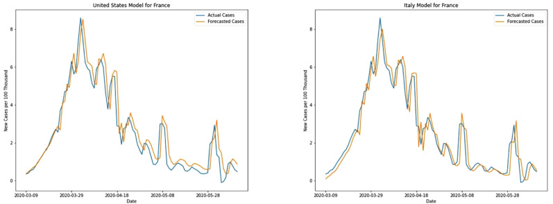
For new cases, the Italy model performs slightly better for France as compared to the US models. The differences in the result are prominent in the first peak occurring around the end of March, where the US model predicts higher values than the Italy model. France imposed lockdown from March 17th [17] when both new cases and death cases were having a very steep rise. Within a week both the curves for new cases and new deaths reached its’ peak and started descending gradually. As new cases started leveling out, France eased its lockdown from the first week of May with strict controls in hotspots of the spread. Both US and Italy models predict well for all different cases like steep rise, peak, and the gradual descent of new cases of curves (see Fig. 4). The Italy model has MAE of 0.46 and RMSE of 0.69 compared to MAE and RMSE of 0.49 and 0.7 respectively for the US model.
Fig. 4.
New cases prediction for France.
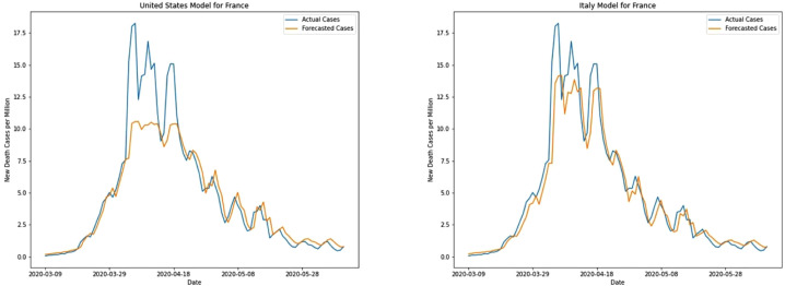
The Italy model performs better for new death cases of France with an MAE of 0.84 compared to the US model’s MAE of 1.15. Even though both the models perform comparatively well in the initial gradual rise and later gradual descend of death cases, the US model fails to forecast the steep peaks during April as seen in Fig. 5.
Fig. 5.
New death cases prediction for France.
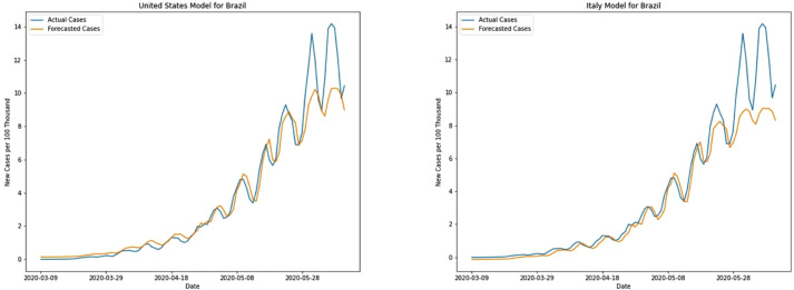
Both the models’ forecasts for Brazil have small errors initially as there is a gradual rise in new cases. However, during mid-May as there is a very steep rise in cases both the models fail to capture the steep peak which is visible in graphs of Fig. 6. Even though the US model predicts better in these peaks the error is still very high compared to prediction in other test countries.
Fig. 6.
New cases prediction for Brazil.
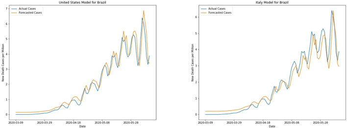
Unlike the forecast for new cases, both models can forecast new death cases for Brazil comparatively better (see Fig. 7). Numerically, the US model performs better with the MAE of 0.23. Unlike the case of France, both the models can forecast well in the peak region of Brazil.
Fig. 7.
New death cases prediction for Brazil.
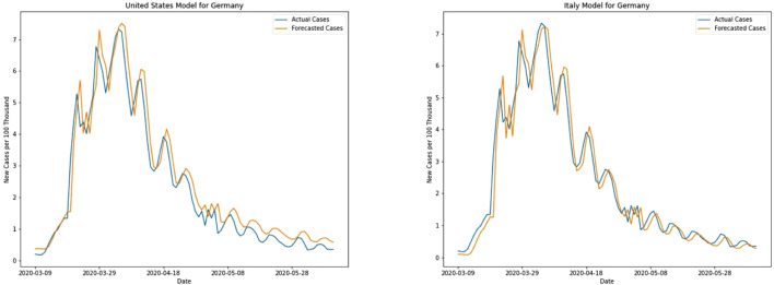
Germany’s infection curves are limited compared to other European nation mainly because of its’ quick actions and strict regulations. Beginning at the start of March itself strict regulations were being imposed for gathering [17] and offices. The Italy model performs better for Germany with an MAE of 0.32 compared to 0.97 for the US model. US model generally predicts higher values and the differences are clearer in May in Fig. 8 when new cases have started decreasing gradually.
Fig. 8.
New cases prediction for Germany.
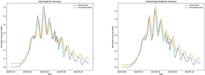
New death cases start to decrease after mid-April in Germany, Both the models predict higher values during this instance (see Fig. 9). Germany comparatively has a lower mortality rate compared to other similarly infected EU countries like Italy and France. Numerically, the US model predicts better in terms of MAE (0.23) compared to 0.24 of the Italy model, though the Italy model’s RMSE of 0.30 is less than that of the US model (0.32).
Fig. 9.
New death cases prediction for Germany.
For Germany, though the Italy model predicts better for new cases, the US model predicts better for death cases. A possible explanation can be provided from training data. If we visualize the training data for Italy and United States in Fig. 2, Fig. 3, it can be observed that for the United States’ new cases, gradual descent is still not distinctly visible as in Italy and Germany. In contrast, gradual descent is clear for new death cases in the United States data. Because of this United States’ training data for new death cases can capture a wider range of patterns than the data for new cases which still have no signs of the descent part. Moreover, the death cases data for the United States and Germany has a clear waveform with seasonal ups and downs which is not so clear in Italy’s data. This similarity in the US and Germany could also be a reason for the ability of the US model to perform better than the Italy model for death cases of Germany.
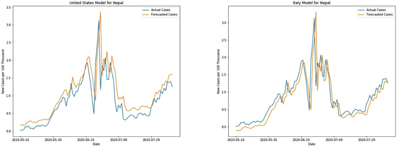
Nepal was under lockdown from March 24th and the easing started only around June 10th and finally ending it officially July 21st. Even then national and international flights have yet not started, inter-district mobility is highly controlled and strict restrictions apply to public gatherings. Vehicle movement has been controlled heavily using odd–even number plate rule, where only odd-numbered or even-numbered plates are allowed in a single day. Moreover, areas reporting higher cases have been put under immediate seal. Because of all these strict measures, the highest new cases reporting is limited to a few hundred. The new death cases are also limited to single-digit figures. However, even for such low cases, both models perform pretty well with MAE of 0.22 and 0.25 for Italy and US model respectively. Fig. 10 depicts the differences between these two models, Italy model predicts lower values for most of the instances whereas the US model predicts higher values.
Fig. 10.
New cases prediction for Nepal.
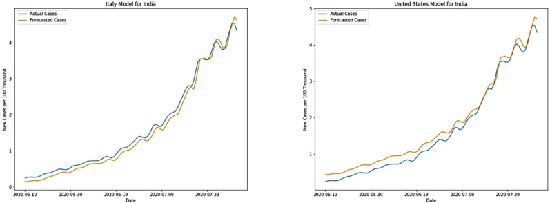
Though India maintained a longer lockdown in various phases easing different sectors one by one, the virus spread has gradually increased reaching threatening numbers. Sharp peaks are still not visible and it is still gradually increasing. For new cases, both the models have a modest performance with MAE of 0.12 and 0.17 for Italy and US models respectively. As seen in other test countries the US model predicts higher values compared to the Italy model (see Fig. 11).
Fig. 11.
New cases prediction for India.
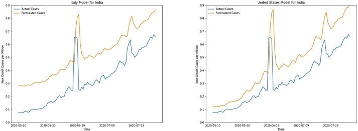
US model has an MAE of 0.138 for India which is the best figure among all the test countries for new death cases. Italy model also has a pretty decent MAE of 0.2 however it can be seen in Fig. 12 that initially Italy model has higher forecasted values with nearly equal forecasted values later for both the models as cases reach higher values.
Fig. 12.
New death cases prediction for India.
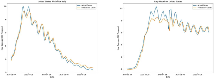
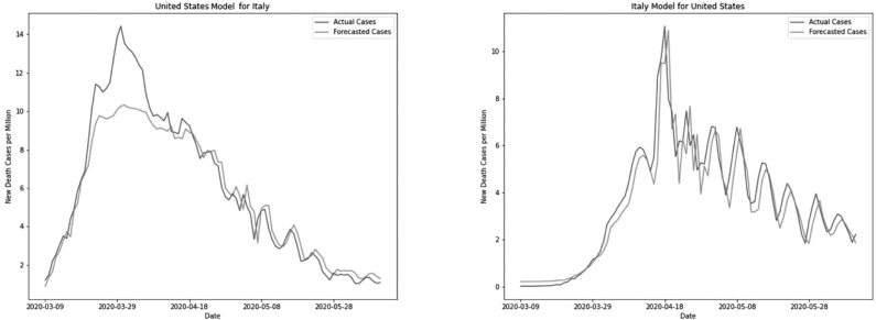
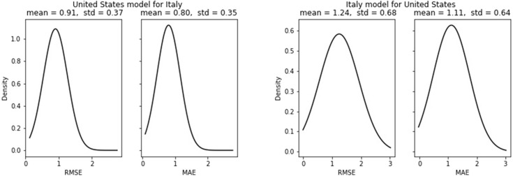
For new cases, Italy and US models when tested in each other produce interesting results. US model predicts comparatively better for Italy with MAE of 0.37, capturing its steep rise and peak very closely. Italy model on the other hand fails to capture sharp peaks in US Data and has an MAE of 0.56. The difference can be visualized more vividly in Fig. 13.
Fig. 13.
New cases prediction for Italy and the United States.
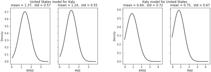
For new death cases, the US model has a higher error for Italy as compared to the Italy model’s error for the US. The errors are more pronounced in steep peaks of Italy occurring during the end of March (see Fig. 14). However, the Italy model predicts closely in the peak region of the US occurring during mid-April and other consecutive smaller peaks occurring thereafter.
Fig. 14.
New death cases prediction for Italy and the United States.
The Italy model predicts pretty well for countries like France, Germany whereas it predicts lower values for countries like Brazil and the United States and thus has comparatively large RMSE and MAE. The strategies implemented in European countries were pretty similar to each other [18], so the Italy model predicts better for European countries whereas for Brazil the strategy was very different from that of Italy and the US as well so the forecasts have higher errors. However, for Countries like Nepal and India where there are a lot of differences in intervention strategy, the health care system, and other control policies Italy model performs just as well as it performed for the European countries. This shows the forecasted values are also a strong function of its history or past data regardless of the exact policies being implemented or the other diversifying factors.
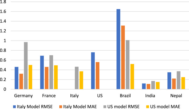
The lowest RMSE and MAE of the Italy model are 0.12 and 0.11 respectively both occurring for India, and the maximum value is 1.31 and 1.65 respectively occurring in Brazil for new cases. The lowest RMSE and MAE of the US model are also for India with 0.17 and 0.15 respectively. One of the possible reasons for this can be India is having a gradual rise in cases and still not seen steep peaks where the models’ performance is compromised. It can be seen in the earlier forecast figures, both the models’ weakness lies in peaks but performs extremely well on gradual incline or decline of cases.
The graphs of new cases for France, Italy, Germany, and Brazil consist of clear spikes which represent the highest rise in cases, the models predict fine for all these peaks except for Brazil. Thus, the models are not able to forecast a very steep rise in cases in Brazil. The graphs for Brazil depict the US model has a better capacity to encapsulate sharp spikes better than the Italy model for new cases. In contrast, the Italy model better encapsulates sharp spikes in death cases better compared to US models.
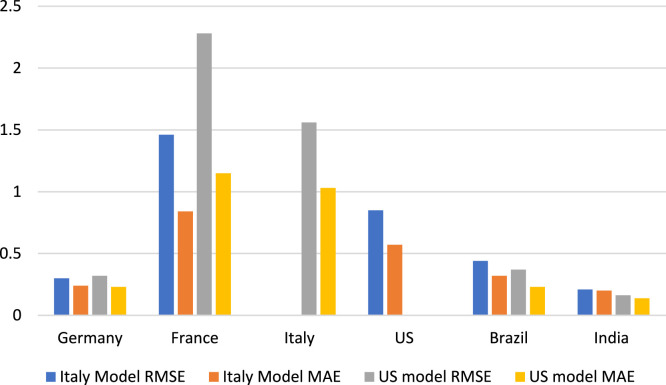
The difference in MAE and RMSE for both the models in various countries can be visualized through Fig. 15, Fig. 16. For testing purposes, training data i.e. Italy and US data have not been used for error analysis in Italy and US models respectively as these are the training data for the respective models.
Fig. 15.
Single day new cases forecast error.
Fig. 16.
New death cases forecast errors.
3.1.2. Multi-step forecast
The same set of data has been used for the multistep forecast as in single-step forecasts. Total data of 102 days form 78 test sets for the five-days forecast. The mean value of RMSE and MAE across all these sets is calculated along with its standard deviation. The result is then fitted to a normal distribution for analyzing the variability in error across these test sets. The model requires 25 days of data, for single set validation, 20 for window size, and 5 for forecasts.
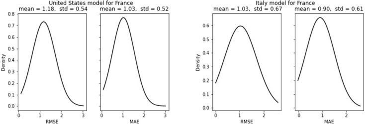
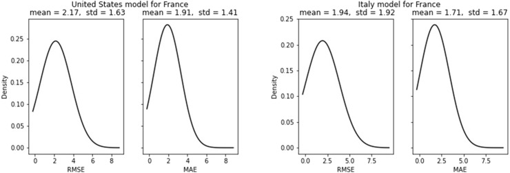
As for the single day forecast of France, the results of both models have a very small difference. Though the error parameters are small, it is nearly twice compared to the single-step forecast. The forecast results for new death cases are unacceptably large with very high MAE and RMSE along with high deviation for both the models (see Fig. 17, Fig. 18). The distributions extend to numbers as high as 7 which has not been recorded for other test countries.
Fig. 17.
New cases forecast error for France.
Fig. 18.
New death cases forecast error for France.
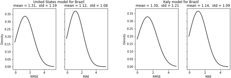
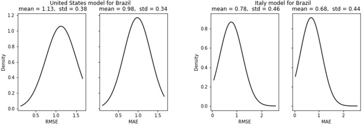
With MAE of 1.12 and 1.14 for US and Italy models respectively for new cases, the forecasted errors for Brazil are nearly equal for both the models. Though the US model performed comparatively better for single-step prediction the results for multistep prediction have one of the highest errors compared to other test countries. However, the results for new death cases are quite contrasting as the results are better compared to other test countries (see Fig. 19, Fig. 20).
Fig. 19.
New cases forecast error for Brazil.
Fig. 20.
New death cases forecast error for Brazil.
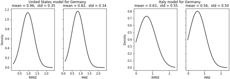
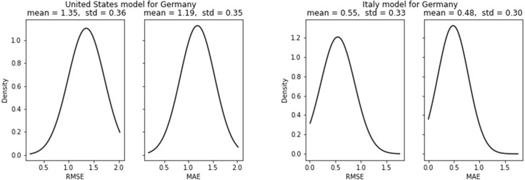
Consistent with the single-step prediction for Germany, Italy model has a modest performance for multistep new cases prediction with an MAE of 0.56 while the US model has an MAE of 0.82. The standard deviation for US and Italy models for MAE is 0.50 and 0.34 respectively, the results are stable across the test set. The performance of Italy models for new death cases is even better with an MAE of 0.48 and a standard deviation of 0.30, the results are quite stable across the test set (see Fig. 21, Fig. 22).
Fig. 21.
New cases forecast error for Germany.
Fig. 22.
New death cases forecast error for Germany.
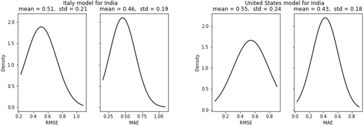
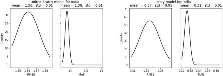
In case of India, though the Italy model has slightly better performance, both the models have a similar distribution with nearly equal error and its deviation (see Fig. 23). Compared to other countries MAE of 0.46 and 0.43 are modest numbers however compared to India’s single-step prediction the figures are nearly four times higher. For new death cases, both the models have the least deviated results with a standard deviation of 0.01 for both MAE and RMSE (see Fig. 24).
Fig. 23.
New cases forecast error for India.
Fig. 24.
New death cases forecast error for India.
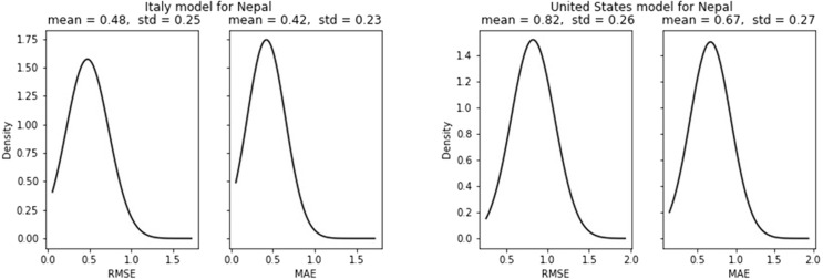
Italy model for Nepal has the best performance compared to all the test countries with an MAE of 0.42 Nepal is still in its early phase with a very slow gradual rise in cases. It has been seen in the single-step prediction that both the models predict well in regions of gradual rise or fall and have some compromise in predictions near the peaks. As Nepal does not have any sharp spikes and peaks this may be the reason for Italy’s fine performance for Nepal (see Fig. 25).
Fig. 25.
New cases forecast error for Nepal.
Consistent with the single-step prediction of new cases, the US model performs better for Italy compared to the Italy model’s performance for the United States. And for new death cases, the Italy model performs better for the United States (see Fig. 26, Fig. 27).
Fig. 26.
New cases forecast error for Italy and US.
Fig. 27.
New death cases forecast error for US and Italy.
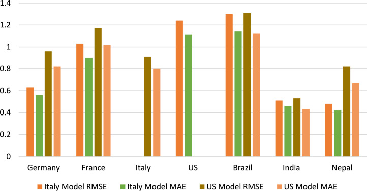
The lowest RMSE (0.48) and MAE (0.42) for Italy model’s new cases are for Nepal. The standard deviation for RMSE is 0.21 and MAE is 0.19, which are also pretty low, meaning the error does not deviate much through all of its test sets and the forecasts are stable. The Italy model also performs well for Germany as in single-step predictions. Moreover, the Italy model’s RMSE (1.3) and MAE (1.14) is high for Brazil. Unlike in single-step prediction, the Italy model does not predict well for France as it is RMSE(1.03) and MAE (0.9) are comparatively higher.
For new cases, Lowest RMSE (0.53) and lowest MAE (0.43) for the US model are seen for India, which is comparatively higher than errors observed in the Italy model. Like the Italy model, the US model also fails to predict better for Brazil. The RMSE and MAE values for Brazil are 1.31 and 1.12 respectively which is nearly equal to that of the Italy model.
Except for India and Germany both the models predict on a similar scale for new cases. The inability of the models to predict well for Brazil’s new cases may be explained by the problems in its different restriction policies. The strategy followed in Brazil is very different from to rest of the world [19] and has a very steep rise in new cases and death cases as well which may be the reason for higher prediction error. Moreover, Brazil shows a higher variation in error which can be visualized in Fig. 19, Fig. 20.
As expected, the 5 days models do not perform as good as single day models, as it is more challenging to capture and forecast long ranger patterns than a shorter one. Even then the results are satisfying for countries like India and Germany for new cases.
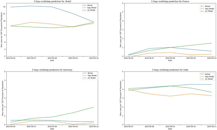
5 days new cases prediction error can be visualized from Fig. 28. Italy’s model performance for Nepal is far better than any other prediction model both. Samples of a multistep forecast for new cases have been presented in Fig. 29.
Fig. 28.
New cases multistep forecast error.
Fig. 29.
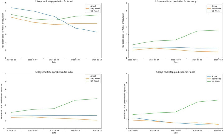
Samples of multistep forecast for new cases.
Though any conclusion cannot be drawn from samples of Fig. 29, what can be observed is the US model has predicted higher values compared to both the actual value and values forecasted by the Italy model.
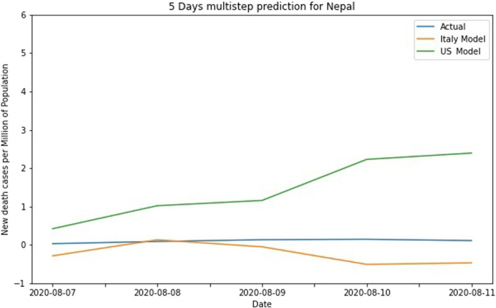
Fig. 30 depicts the multistep forecast for the latest available values for Nepal. The cases in Nepal are gradually rising and still, the spread is in its’ initial phase. For Nepal also US model predicts higher values compared to Italy’s model. As for available data for new death cases of Nepal, it is still limited to single-digit figures and there are many days with no new death cases recorded. So, forecasts for new death cases have not been presented as the numbers are too close to zero and will be ambiguous to compare with the results of other test countries.
Fig. 30.
New cases multistep forecast for Nepal.
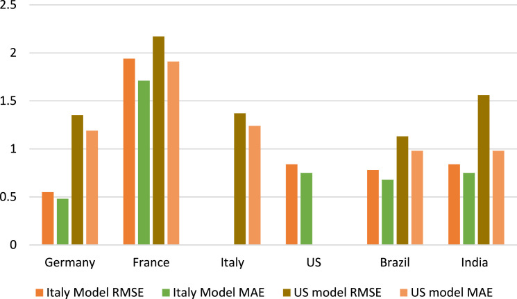
Error for multistep death cases forecast can be visualized in Fig. 31. In contrast to all previous forecasts, Brazil also has achieved decent results. For new death cases, the best result is obtained for the Italy model applied to Germany with MAE of 0.48 and RMSE of 0.55. Both US and Italy models have poor performance for France with the highest MAE of 1.71 and 1.91 respectively for Italy and the US model. For all the test countries Italy model’s performance is numerically better than that of the US model. Samples of multistep forecast are presented in Fig. 32.
Fig. 31.
New death cases multistep forecast error.
Fig. 32.
Samples of multistep forecast for new death cases.
As expected, multistep models have higher errors than single-step models for both new cases and deaths forecast as capturing longer sequences is challenging. Even then good results have been obtained for countries like Germany, Nepal, and India for new cases and Brazil and Germany for death cases. The results can further be improved by considering other variables like age ratio, population density, and localizing the forecasts to a particular region of hotspots like New York, Delhi, Paris, etc. With such limited training data and wide diversity across the test countries, the proposed models have provided a decent forecast.
4. Conclusions
In this paper, Transfer Learning is applied in the LSTM network to learn trends of new cases and new deaths because of COVID-19 from data of Italy and the United States and forecast for other countries. Germany, France, Brazil, India, and Nepal have been tested for single-step and multistep predictions from the prepared models. These forecasts have verified that even for different modes of intervention, policies, and health care systems, the proposed models can predict well. The results indicate new cases and deaths can be forecasted pretty well with the proposed models. Complex patterns of steep rise, spikes, and flattening effects of new cases and deaths can be learned from mature datasets i.e. data from countries infected earlier. This approach is more useful for countries that are in its early phase of virus spread, to forecast based on other country’s models. Such forecasts can be a great help to governments and policymakers.
Declaration of Competing Interest
The authors declare that they have no known competing financial interests or personal relationships that could have appeared to influence the work reported in this paper.
References
- 1.2020. Coronavirus Update (Live): 20, 514, 016 Cases and 745, 687 Deaths from COVID-19 Virus Pandemic - Worldometer. https://www.worldometers.info/coronavirus/. [Accessed 12 August 2020] [Google Scholar]
- 2.Atalan A. Is the lockdown important to prevent the COVID-9 pandemic? Effects on psychology, environment and economy-perspective. Ann Med Surg. 2020 doi: 10.1016/j.amsu.2020.06.010. [DOI] [PMC free article] [PubMed] [Google Scholar]
- 3.Liu Y.C., Kuo R.L., Shih S.R. COVID-19: The first documented coronavirus pandemic in history. Biomed J. 2020:1–6. doi: 10.1016/j.bj.2020.04.007. [DOI] [PMC free article] [PubMed] [Google Scholar]
- 4.Swapnarekha H., Behera H.S., Nayak J., Naik B. Role of intelligent computing in COVID-19 prognosis: A state-of-the-art review. Chaos Solitons Fractals. 2020;138 doi: 10.1016/j.chaos.2020.109947. [DOI] [PMC free article] [PubMed] [Google Scholar]
- 5.Ben Fredj H., Chrif F. Novel Corona virus Disease infection in Tunisia: Mathematical model and the impact of the quarantine strategy. Chaos Solitons Fractals. 2020 doi: 10.1016/j.chaos.2020.109969. [DOI] [PMC free article] [PubMed] [Google Scholar]
- 6.Torrealba-Rodriguez O., Conde-Gutiérrez R.A., Hernández-Javier A.L. Modeling and prediction of COVID-19 in Mexico applying mathematical and computational models. Chaos Solitons Fractals. 2020:138. doi: 10.1016/j.chaos.2020.109946. [DOI] [PMC free article] [PubMed] [Google Scholar]
- 7.Ndaïrou F., Area I., Nieto J.J., Torres D.F.M. Mathematical modeling of COVID-19 transmission dynamics with a case study of Wuhan. Chaos Solitons Fractals. 2020:135. doi: 10.1016/j.chaos.2020.109846. [DOI] [PMC free article] [PubMed] [Google Scholar]
- 8.Tomar A., Gupta N. Prediction for the spread of COVID-19 in India and effectiveness of preventive measures. Sci Total Environ. 2020;728 doi: 10.1016/j.scitotenv.2020.138762. [DOI] [PMC free article] [PubMed] [Google Scholar]
- 9.Chimmula V.K.R., Zhang L. Time series forecasting of COVID-19 transmission in Canada using LSTM networks. Chaos Solitons Fractals. 2020:135. doi: 10.1016/j.chaos.2020.109864. [DOI] [PMC free article] [PubMed] [Google Scholar]
- 10.Ghosal S., Bhattacharyya R., Majumder M. Impact of complete lockdown on total infection and death rates: A hierarchical cluster analysis. Diabetes Metab Syndr Clin Res Rev. 2020;14:707–711. doi: 10.1016/j.dsx.2020.05.026. [DOI] [PMC free article] [PubMed] [Google Scholar]
- 11.Roser M., Ritchie H., Ortiz-Ospina E., Hasell J. Coronavirus Pandemic (COVID-19) Our world data. 2020 [Google Scholar]
- 12.Connor J.T., Martin R.D., Atlas L.E. Recurrent neural networks and robust time series prediction. IEEE Trans Neural Netw. 1994;5:240–254. doi: 10.1109/72.279188. [DOI] [PubMed] [Google Scholar]
- 13.Pascanu R, Mikolov T, Bengio Y. On the difficulty of training recurrent neural networks. In: 30th int conf mach learn; 2013, p. 2347–55.
- 14.Hochreiter S., Schmidhuber J. LSTM can solve hard long time lag problems. Adv Neural Inf Process Syst. 1997:473–479. [Google Scholar]
- 15.2020. Keras: the Python deep learning API. https://keras.io/, [Accessed 16 June 2020] [Google Scholar]
- 16.2020. Welcome To Colaboratory - Colaboratory. https://colab.research.google.com/notebooks/intro.ipynb, [Accessed 17 June 2020] [Google Scholar]
- 17.2020. Coronavirus: France eases lockdown after eight weeks - BBC News. https://www.bbc.com/news/world-europe-52615733, [Accessed 15 August 2020] [Google Scholar]
- 18.Meunier T. 2020. Full lockdown policies in Western Europe countries have no evident impacts on the COVID-19 epidemic. [DOI] [Google Scholar]
- 19.2020. Coronavirus quarantine: While other countries open up, Brazil can’t lock down - The Washington Post. https://www.washingtonpost.com/world/while-other-countries-look-to-open-up-brazil-cant-find-a-way-to-shut-down/2020/05/10/2c02abea-92c1-11ea-87a3-22d324235636_story.html, [Accessed 17 June 2020] [Google Scholar]


