Multi-window back-projection residual networks for reconstructing COVID-19 CT super-resolution images

Abstract

Background and objective

With the increasing problem of coronavirus disease 2019 (COVID-19) in the world, improving the image resolution of COVID-19 computed tomography (CT) becomes a very important task. At present, single-image super-resolution (SISR) models based on convolutional neural networks (CNN) generally have problems such as the loss of high-frequency information and the large size of the model due to the deep network structure.

Methods

In this work, we propose an optimization model based on multi-window back-projection residual network (MWSR), which outperforms most of the state-of-the-art methods. Firstly, we use multi-window to refine the same feature map at the same time to obtain richer high/low frequency information, and fuse and filter out the features needed by the deep network. Then, we develop a back-projection network based on the dilated convolution, using up-projection and down-projection modules to extract image features. Finally, we merge several repeated and continuous residual modules with global features, merge the information flow through the network, and input them to the reconstruction module.

Results

The proposed method shows the superiority over the state-of-the-art methods on the benchmark dataset, and generates clear COVID-19 CT super-resolution images.

Conclusion

Both subjective visual effects and objective evaluation indicators are improved, and the model specifications are optimized. Therefore, the MWSR method can improve the clarity of CT images of COVID-19 and effectively assist the diagnosis and quantitative assessment of COVID-19.

1. Introduction

After the coronavirus invaded the lungs, it would diffuse along alveolar pores, which would lead to alveolar swelling, exudation of alveolar septum fluids, and thickening of alveolar septum, etc. All these will increase the CT number of the lungs, namely the lungs will become white. There is no exudation of granulocytes in viral infections, the alveoli are clean, and the air is still inside, so there is often a ground glass shadow without a substantial white mass change. Therefore, super-resolution (SR) reconstruction technology is urgently needed to improve the resolution of COVID-CT as an important basis for the diagnosis of COVID-19 [1].

Single-image super-resolution (SISR) reconstruction is an important image processing technology in the field of computer vision, which is widely used in medicine, video, security, and remote sensing. In the actual scene, due to the limitations of the existing medical hardware conditions, low-quality low-resolution (LR) medical images are often obtained. For example, the medical images of the current hospital CT detector as the detection and diagnosis of diseases often lack the key detection details or parts of the scene. Therefore, it is necessary to overcome the resolution limitations of the existing hardware system and use SISR reconstruction technology for enhancement the spatial resolution of the image. The core idea of this technology is to reconstruct the super-resolution image with high pixel density by analyzing the key semantic information or signal information of LR image, inferring the lack of real details.

At present, the research of SISR reconstruction is mainly divided into three stages. The earliest and most intuitive method is interpolation method based on sampling theory [2,3]. The advantage of this method is that it runs fast and is suitable for parallel computing, but it can't introduce additional useful high-frequency information, so it is difficult to get sharp high-definition image.

After that, some scholars proposed that the information of the corresponding high-resolution (HR) part can be inferred from the LR image. Relying on the technique of neighborhood embedding [4,5], sparse coding [6], [7], [8], the algorithm of learning the mapping function between LR image and HR image is studied and proposed. However, when the image does not contain enough repetitive patterns, this method tends to produce non-detailed sharp edges.

The main contributions of this paper are described as follows:

• (1)Expand the network structure horizontally to avoid the vertical depth of the network. The extended network uses the multi-window up-projection and down-projection residual module (MWUD) to extract the key information of the same feature map at the same time from the shallow network, to obtain more complete high/low frequency information in the original image as soon as possible.
• (2)The residual network extracts features. The dilated convolution is used to expand the receptive field, and the image high/low frequency information is extracted layer by layer through 3 repetitive and continuous residual modules.

2. Deep neural network for super-resolution reconstruction

In recent years, methods based on deep learning have become the most active research direction in the field of SR. Since the SRCNN [9] model proposed by Dong C et al. successfully used the convolutional neural network technology to reconstruct and generate higher-definition images, such methods have come to the fore. It uses many external HR images to construct a learning library, and generates a neural network model after training. In the process of LR image reconstruction, the prior knowledge obtained by the model is introduced to obtain the high-frequency detail information of the image, to achieve the excellent image reconstruction effect.

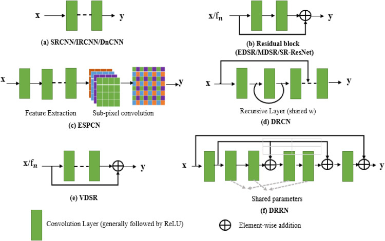
After that, FSRCNN [10], ESPCN [11] and other models have made some improvements on each part of the network structure based on SRCNN, and increased the number of network layers, focusing on learning the end-to-end mapping relationship from LR images to HR images, as shown in Fig. 1 . However, with the deepening of the network layer, the training cost increases gradually. At the same time, due to the increase of channel number, filter size, step size and other super parameters, it is very difficult to design a reasonable network structure. Then, He et al. [12] proposed the ResNet to solve the above problems. Although it is suitable for image classification, its residual idea and strategy of repeated stacking modules can be applied to all computer vision tasks. In addition, the ResNet also proved that shortcut connection and recursive convolution can effectively reduce the burden of neural network carrying a lot of key information.

Fig. 1.

Single image super-resolution network architecture of deep network.

Subsequently, residual network based super-resolution models, such as DRCN [13], DRNN [14], LapSRN [15], SRResNet [16], and EDSR [17] have been proposed, as shown in Fig. 1. These models are implemented by linear superposition of single size convolution modules to achieve the vertical deepening of the network, to pursue higher expression and abstract ability. However, for the super-resolution technology, it is very important to extract rich and complete feature information from the original image. If the network is deepened vertically, the high frequency information will be lost in the process of layer-by-layer convolution and filtering calculation, which will affect the authenticity of the final mapping generated super-resolution image. In addition, the number of model parameters will also increase exponentially. If the training dataset is limited, it is easy to produce over fitting; the model specifications will increase, and it is not easy to reconstruct and transplant; the amount of calculation will also increase, resulting in the training difficulty multiplied and difficult to apply.

3. Multi-window back-projection residual networks

To solve the problems of incomplete extraction of feature information in the original input image and large model scale due to the deep longitudinal structure of the network, we propose a multi-window back-projection residual networks for reconstructing COVID-19 CT super-resolution images. The model mainly includes multi-window up-projection and down-projection residual module (MWUD) and 3 Residual block modules (RB), MWUD is up-projection and down-projection residual module, RB is residual block module. as shown in Fig. 2 .

Fig. 2.

The architect of multi-window back-projection networks.

3.1. Multi-window up-projection and down-projection residual module

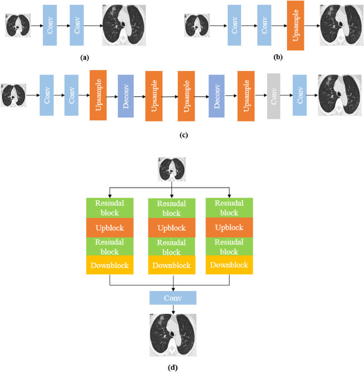
In the deep network, it is divided into three types. Fig. 3 is (a) Predefined upsampling, (b) Single upsampling, (c) Progressive upsampling. In this article, we proposed the multi-window up-projection and down-projection residual module, as shown in Fig. 3(d).

Fig. 3.

Comparisons of deep network super-resolution. (a) Predefined upsampling (e.g., VDSR [18], DRRN [18], SRCNN [9]). (b) Single upsampling (e.g., ESPCN [11], FSRCNN [10]). (c) Progressive upsampling uses a Laplacian pyramid network. (d) multi-window up-projection and down-projection rsidual module is proposed by our MWSR which uses the interconnected up- and down sampling stages to obtain many HR features of different depths.

The main purpose of multi-window up-projection and down-projection residual module (MWUD) is to explore the interdependence between LR and HR as an efficient iterative process. In addition, the MWUD module can provide more information for each bottom-up or top-down mapping and increase the flow of information. When the sampling multiple is large, the corresponding size of convolution kernel or deconvolution kernel is large, which makes the convergence speed of network slow and easy to fall into suboptimal results [20]. In each MWUD, the use of skip connections to fuse intermediate-scale features and the use of 1×1 convolution kernel to reduce the dimensionality of the fused high-dimensional features improve the feature utilization rate reduces the complexity of the network, which can obviously optimize the network structure.

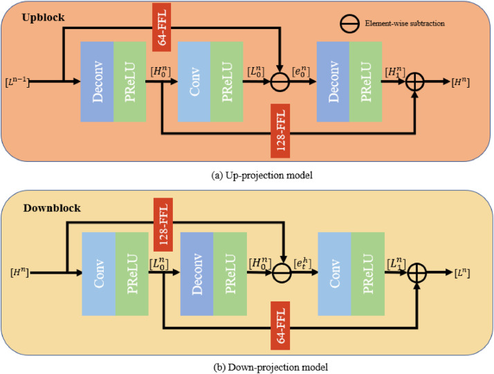
As shown in Fig. 3 (d), multi-window back-projection network consists of three up-projection and down-projection residual modules, each MWUD module consists of an up-projection (upblock), a down-projection (downblock), and two residual block modules. Consequently, in the deep network, in order to increase the receptive field and reduce the amount of calculation, it is necessary to carry out subsampled (pooling or S2 / conv). Although the receptive field can be increased, the spatial resolution is reduced. In this paper, we introduce dilated convolution into the up projection and down-projection of MWUD module without losing the resolution and expanding the receptive field. Furthermore, 128 feature fusing layer and 64 Feature Fusing Layers (FFL) are introduced in up-projection model and down-projection model to reduce the MWSR network parameters, the parameters are shown in Table 1 . In the MWUD module, different division rates lead to different receptive fields, which can capture multi-scale context information of COVID-19 CT images.

Table 1.

The network architect setting of MWSR.

Network module			Kernel size	Stride	Padding	Dialted rate	Input size	Output size
Initial layer			3*3	1	1	1	H*W*1	H*W*64
Residual block		Conv 1	3*3	1	1	1	H*W*64	H*W*64
		Conv 2	1*1	1	0	1	H*W*64	H*W*4
		Conv 3	1*1	1	0	1	H*W*4	H*W*64
Upblock	1	DeConv	4*4	2	1	1	H*W*64	H*W*128
		Conv	4*4	2	1	1	H*W*128	H*W*64
		DeConv	4*4	2	1	1	H*W*64	H*W*128
	2	DeConv	4*4	2	4	3	H*W*64	H*W*128
		Conv	4*4	2	4	3	H*W*128	H*W*64
		DeConv	4*4	2	4	3	H*W*64	H*W*128
	3	DeConv	4*4	2	7	5	H*W*64	H*W*128
Conv		4*4	2	7	5	H*W*128	H*W*64
DeConv		4*4	2	7	5	H*W*64	H*W*128
Downblock	1	Conv	4*4	2	1	1	H*W*128	H*W*64
		DeConv	4*4	2	1	1	H*W*64	H*W*128
		Conv	4*4	2	1	1	H*W*128	H*W*64
	2	Conv	4*4	2	4	3	H*W*128	H*W*64
		DeConv	4*4	2	4	3	H*W*64	H*W*128
		Conv	4*4	2	4	3	H*W*128	H*W*64
	3	Conv	4*4	2	7	5	H*W*128	H*W*64
DeConv		4*4	2	7	5	H*W*64	H*W*128
Conv		4*4	2	7	5	H*W*128	H*W*64
RB module		Conv 7	3*3	1	1	1	H*W*64	H*W*64
		Conv 8	1*1	1	0	1	H*W*64	H*W*4
		Conv 9	1*1	1	0	0	H*W*4	H*W*64
Middle layer			3*3	1	1	1	H*W*64	H*W*64
Upscale			3*3	1	1	1	H*W*64	2H*2W*64
Reconstruction layer			3*3	1	1	1	2H*2W*64	2H*2W*1

The up-projection model maps each other step by step between the LR feature map and the HR feature map, and the down-projection model maps each other step by step between the HR feature map and the LR feature map, as shown in Fig. 4 . Accordingly, back-projection extracts image features by up-projection and down-projection. It can be understood that the network is a process of continuous self-correction. Its purpose is to avoid the single-step nonlinear mapping error when only up-sampling at the end of the network [20], and to improve the super-resolution performance.

Fig. 4.

Structure of up-projection model and down-projection model.

Furthermore, the input of up-projection model is a LR feature map, which is mapped three times between the LR image and the HR image. The three mappings are: the first mapping maps the LR feature map to the HR feature map, the second mapping maps from the HR feature map to the LR feature map, and the third mapping maps the LR feature map to the HR feature map for output. Meanwhile, the down-projection model is very similar to the up-projection model, which is the inverse process of the up-projection model. Thus, the input of the down-projection model is a HR feature map, and after three mappings, the final output is a LR feature map.

The up-projection and down-projection residual module are defined as follows: up-projection scale up:

$$H_0^{\mathrm{n}}=\left(L^{n-1}*p_{\mathrm{n}}\right){\uparrow }^s$$ (1)

up-projection scale down:

$$L_0^{\mathrm{n}}=(H_0^{\mathrm{n}}*g_{\mathrm{n}}){\downarrow }_s,$$ (2)

up-projection residual:

$${\mathrm{e}}_{\mathrm{n}}^1=L_o^n-L^{n-1},$$ (3)

up-projection scale residual up:

$$H_1^{\mathrm{n}}=\left({\mathrm{e}}_n^1*q_{\mathrm{n}}\right){\uparrow }^s,$$ (4)

output feature map:

$$H^{\mathrm{n}}=H_0^{\mathrm{n}}+H_1^{\mathrm{n}},$$ (5)

down-projection scale down:

$$L_1^{\mathrm{n}}=\left(H_2^{\mathrm{n}}*g_n\right){\downarrow }_s,$$ (6)

down-projection scale up:

$$H_3^{\mathrm{n}}=\left(L_1^{\mathrm{n}}*p_n\right){\uparrow }^s,$$ (7)

down-projection residual:

$$e_h^n=H_3^n-\left(H_2^n*k_n\right),$$ (8)

down-projection scale up:

$$H_3^{\mathrm{n}}=\left(L_1^{\mathrm{n}}*p_{\mathrm{n}}\right){\uparrow }^s,$$ (9)

down-projection scale residual up:

$$L_2^{\mathrm{n}}=\left(e_{\mathrm{h}}^{\mathrm{n}}*g_n\right){\downarrow }_s,$$ (10)

output feature map:

$$L^n=L_0^n+L_1^n,$$ (11)

where * is the convolution operation. ↑^s and ↓_s are the upsampling and subsampled operation with scale factor S, respectively. p_n is the upsampling deconvolutional layer of the n − th UD. g_n is the subsampled convolutional layer of the n − th UD. q_n is 128-dimensional feature fusion layer of the n − th UD. k_n is 64-dimensional feature fusion layer of the n − th UD [21].

3.2. Residual block module

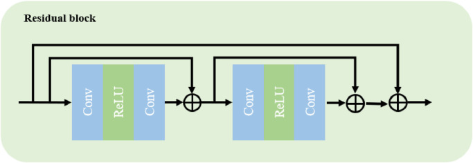
The MWSR model extracts the high and low frequency information of the image layer by layer through three repeated and continuous residual blocks, and fuses the initial feature map and the output of the above three residual blocks to merge the information flow through the network into the reconstruction module [22,23]. Thus, we construct three RB modules to extract deep features, as shown in Fig. 5 . The operation of RB can be described as:

$$T=[Q_3^1,M_1,M_2,M_3],$$ (12)

where [ ] is the connection operation between features, $Q_3^1$ is the initial feature graph, M ₃ is the output of the third residual module, and T is the output of global feature fusion.

Fig. 5.

Structure of residual block model.

3.3. Sub-pixel convolutional upsampling layer

In the actual camera imaging process, due to hardware limitations, each pixel in the generated image represents a whole block of color nearby. In fact, at the microscopic level, there are many pixels, namely sub-pixels, between actual physical pixels. In the field of SR image reconstruction, the sub-pixels that cannot be detected by the sensor can be approximated by algorithms [11], which is equivalent to inferring high-frequency information such as missing texture details in the image.

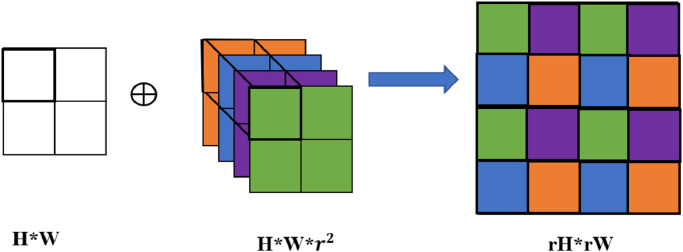
The sub-pixel convolution is used to complete the mapping of LR images to HR images in the high-multiple reconstruction part of the MWSR model, as shown in Fig. 6 . Assuming that the target multiple is γ and the input LR feature map size is H*W, we convolve it with the r² sub-pixel convolution kernel with channel number H*W to obtain H*W*r² pixel values, and then rearrange them to form a target image with size rH*rW.

Fig. 6.

Upsampling process on the subpixel convolution layer.

3.4. Network architect

The proposed the MWSR method is illustrated in Fig. 2. It can be divided into three parts: multi-window back projection, depth feature extraction and sub-pixel convolution layer. Further, set $I_{{}^{LR}}$ and $I_{{}^{LR}}$ denote the input image and the reconstructed image of MWSR, and the input image $I_{{}^{LR}}$ is extracted by an initial layer to obtain the initial feature map $L_{{}^{\text{initial}}}$, C _initial is the initial layer, and the operation of the initial layer can be defined as:

$$L_{\text{in}itial}=C_{initial}*I{}_{LR},$$ (13)

In the multi-window up-projection and down-projection residual modules, MWSR performs the back-projection for the initial feature map L_initial, and the operation of back-projection is described as:

$$L_{bp}=f_{bp}\left(L_{initial}\right),$$ (14)

where f_bp( • ) denotes the operation of back-projection, $I_{{}^{bp}}$ denotes the extracted shallow feature maps by back-projection.

Then, MWSR uses three RB modules to extract deep feature maps from the extracted shallow feature maps, and the operation of deep feature extraction is

$$L_{deep}=f_{deep}\left(L_{bp}\right),$$ (15)

where f_deep( • ) denotes the deep feature extraction operation, L_deep denotes the extracted feature maps by deep feature extraction.

Finally, MWSR uses the sub-pixel convolutional layer to upsample, and the operation of upscaling can be formulated as:

$$L_{up}=f_{up}(L_{initial}+C_{middle}*L_{deep}),$$ (16)

where f_up( • ) denotes the upscaling operation, C_middile denotes the middle layer which is a convolutional layer, L_up denotes the upscaling feature maps.

4. Experiments and analysis

4.1. Dataset and protocol

The public datasets BSD500 and T91 [24] were used in the experiment, and the two training sets have a total of 591 images. Due to the depth model usually benefits from large amounts of data, 591 images are not sufficient to push the model to its best performance [29]. Thus, to make full use of the dataset, we use the MATLAB to expand the data of the BSD500 and T91 training set images by two methods, namely scaling and rotation. Each image was scaled by the ratios of 0.7, 0.8, and 0.9. Additionally, each image was respectively rotated by 90°, 180°, and 270°, and 9456 images were finally obtained. In addition, a lot of tests and comparisons have been made on the public benchmark datasets Set5 [25], Set14 [26], and Urban100 [27].

4.2. Training details and implementation

In this paper, a 48×48 RGB image cut from $I_{{}^{LR}}$ is used as input, and the quality of the generated SR image is evaluated by I_HR of the target magnification. In the proposed MWSR, the parameters are initialized to a gaussian distribution with a mean of 0 and a standard deviation of 0.001, and the initialization of the bias is set to 0. The network trained a total of 200 epochs. To speed up the training process, an adjustable learning rate strategy was used to train the network. The initial learning rate was set to 0.1, and the learning rate decreased to 0.1 times the original learning rate every 10 epochs [30]. When the learning rate decreased to 0.0001, it is then kept at 0.0001 and the batch size is set to 128. In addition, use Adam optimizer [25] to set β₁ = 0.9, β₂ = 0.999, ε = 10⁻⁸ respectively. In this paper, L1 norm is selected as the loss function training model [28]. Compared with L2, it has sparsity, which can realize automatic feature selection, and has fewer parameters, which can better explain the model. L1 loss function to optimize MWSR as follow:

$$L\left(\theta \right)=\frac{1}{N}\sum _{i=1}^N\parallel f_{GBPN}\left(I_{LR}^i\right)-I_{HR}^i|{|}_1,$$ (17)

where θ denotes the parameters of MWSR.

In addition, combined with CUDA 10.0 and PyTorch 1.20, we use Python code to implement MWSR algorithm, and train and evaluate the algorithm through many experiments on NVIDIA GeForce RTX 1080ti GPU and Ubuntu16.04 operating systems.

4.3. Comparison with state-of-the-art methods

We compare our model with the 9 state-of-the-art SR methods, including Bicubic [3], A+ [7], SCN [28], SRCNN [9], FSRCNN [10], VDSR [18], DRCN [13], LapSRN [15], and DRRN [19]. The specific implementation of these models has been officially published on the Internet; thus, these algorithms can be executed on the same test dataset for fair comparison. In addition, the quality of the generated super-resolution image is evaluated by two common objective evaluation indexes: peak signal to noise ratio (PSNR) and structural similarity (SSIM) [31].

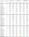
We show the quantitative results in the Table 2 , it shows the evaluation results of 10 kinds of super-resolution algorithms, which are magnified by 2×, 3× and 4× respectively on three public test datasets. As can see that the performance of the MWSR method outperforms other state-of-the art methods in different multiples and different test datasets, further, the MWSR method successfully reconstruct the detailed textures and improves the image perception quality, and realizes the model lightweight and operation efficiency optimization [32]. At the best performance of 2× enlargement on Set14 dataset, the MWSR method achieve 33.53 dB which better 3.28 dB, 1.21 dB, 1.18 dB, 1.02 dB, 0.87 dB, 0.48 dB, 0.47 dB, 0.45 dB, 0.30 dB than Bicubic, A+, SCN, SRCNN, FSRCNN, VDSR, DRCN, LapSRN, and DRRN respectively. Then, to further verify the performance of the MWSR, COVID-19 CT images are used to evaluate the visual quality of MWSR and other state-of-art methods (COVID-CT: https:, github.com/UCSD-AI4H/COVID-CT). The COVID-CT-Dataset has 349 CT images containing clinical findings of COVID-19 from 216 patients, and the images are collected from COVID19-related papers from medRxiv, bioRxiv, NEJM, JAMA, Lancet, etc. CTs containing COVID-19 abnormalities are selected by reading the figure captions in the papers. All copyrights of the data belong to the authors and publishers of these papers.

Table 2.

Quantitative evaluation results of state-of-the-art SR methods: average PSNR and SSIM for scale factors (×2, ×3, ×4). Red numbers indicate the best and green numbers indicate the second-best performance.

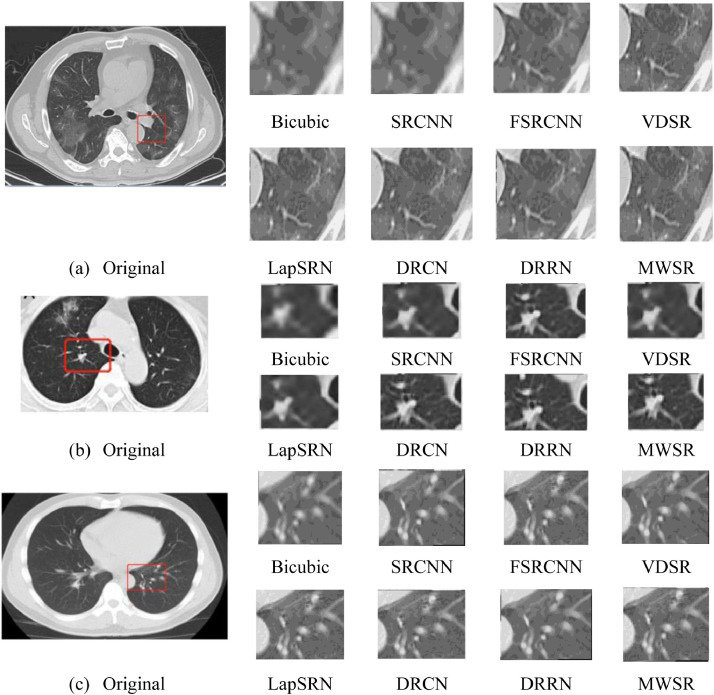
The results of 4× enlargement on the COVID-19 CT images dataset is visually shown in Fig. 7 . By enlarging the reconstructed results in some regions, it can be found that the COVID-19 CT images reconstructed by Bicubic and SRCNN algorithms can hardly observe the contour and other details. While the reconstruction results of FSRCNN, VDSR and LaPSRN algorithms lack the detail information of COVID-19 CT; the reconstruction results of DRCN and DRRN algorithm obtain rich detail information, but lack clear edge information; on the contrary, the COVID-19 CT images reconstructed by the algorithm proposed in this paper can complete the high-frequency information more accurately and completely. Whether it is the detail information or the edge, it can predict the more real new pixel value after magnification according to the overall semantic of the image.

Fig. 7.

Visual quality of the proposed MWSR and other state-of-art methods for 4× scale factor on COVID-19 CT images.

5. Conclusion

In order to solve the problems of incomplete extraction of feature information and large scale of COVID-19 CT original input image due to the deep vertical structure of the network, we propose a super-resolution model based on multi-window back-projection residual networks (MWSR). The model combines three windows to extract the key information of the same feature map at the same time, which can effectively use the feature map of each layer from the shallow network, and improve the probability of detecting high-frequency information. More importantly, compared with the vertical deepening network structure, this horizontal expansion network structure can obtain the complete COVID-19 CT images target features earlier. The experimental results show that MWSR can reconstruct COVID-19 texture features more effectively than other popular models. For future implementation, we will focus on optimizing the up-sampling operation of the high-resolution reconstruction part, and calculate the more realistic and effective mapping relationship between the low-resolution feature space and the high-resolution feature space.

Ethical approval

No ethics approval was required.

Declaration of Competing Interest

The authors declare that they have no conflicts of interest.

References

- 1.Kahrilas PJ, Altman KW, Chang AB, et al. The use of bronchoscopy during the COVID-19 pandemic: CHEST/AABIP guideline and expert panel report. Chest. 2020 S001236921658893X. [Google Scholar]
- 2.Zhang L, Wu X. An edge-guided image interpolation algorithm via directional filtering and data fusion. IEEE Trans. Image Process. 2006;15(8):2226–2238. doi: 10.1109/tip.2006.877407. [DOI] [PubMed] [Google Scholar]
- 3.Qiu D, Zheng L, Zhu J, Han G, Peng Y, et al. Multiple improved residual networks for medical image super-resolution. Future Gen. Comput. Syst. 2021:200–208. [Google Scholar]
- 4.Roweis S T, Saul L K. Nonlinear dimensionality reduction by locally linear embedding. Science. 2000;290(5500):2323–2326. doi: 10.1126/science.290.5500.2323. [DOI] [PubMed] [Google Scholar]
- 5.Gao X, Zhang K, Tao D, et al. Image super-resolution with sparse neighbor embedding. IEEE Trans. Image Process. 2012;21(7):3194–3205. doi: 10.1109/TIP.2012.2190080. [DOI] [PubMed] [Google Scholar]
- 6.Yang J, Wang Z, Lin Z, et al. Coupled dictionary training for image super-resolution. IEEE Trans. Image Process. 2012;21(8):3467–3478. doi: 10.1109/TIP.2012.2192127. [DOI] [PubMed] [Google Scholar]
- 7.Timofte R, Smet Vincent De, Gool Luc Van. Asian Conference on Computer Vision. Springer; Cham: 2014. A+: adjusted anchored neighborhood regression for fast super-resolution; pp. 111–126. [Google Scholar]
- 8.Michael E, Dmitry D. Example-based regularization deployed to super-resolution reconstruction of a single image. Comput. J. 2018;(1):15–30. [Google Scholar]
- 9.Dong C, Loy C C, He K, et al. European Conference on Computer Vision. Springer; Cham: 2014. Learning a deep convolutional network for image super-resolution; pp. 184–199. [Google Scholar]
- 10.Dong C, Loy C C, Tang X, et al. European Conference on Computer Vision. Springer; Amsterdam: 2016. Accelerating the super-resolution convolutional neural network; pp. 391–407. [Google Scholar]
- 11.Shi W, Caballero J, Huszár F, et al. IEEE Conference on Computer Vision and Pattern Recognition. IEEE Computer Society; Las Vegas: 2016. Real-time single image and video super-resolution using an efficient sub-pixel convolutional neural network; pp. 1874–1883. [Google Scholar]
- 12.He K, Zhang X, Ren S, et al. IEEE Conference on Computer Vision and Pattern Recognition. IEEE Computer Society; Las Vegas: 2016. Deep residual learning for image recognition; pp. 770–778. [Google Scholar]
- 13.Kim J, Kwon Lee J, Mu Lee K. Proceedings of the IEEE Conference on Computer Vision and Pattern Recognition. 2016. Deeply-recursive convolutional network for image super-resolution; pp. 1637–1645. [Google Scholar]
- 14.Tai Y, Yang J, Liu X, et al. IEEE Conference on Computer Vision and Pattern Recognition. IEEE Computer Society; Las Vegas: 2017. Image super-resolution via deep recursive residual network; pp. 2790–2798. [Google Scholar]
- 15.Lai W.-S, Huang J.-B, Ahuja N, et al. IEEE Conference on Computer Vision and Pattern Recognition. IEEE Computer Society; Las Vegas: 2017. Deep laplacian pyramid networks for fast and accurate superresolution; pp. 5835–5843. [Google Scholar]
- 16.Ledig C, Wang Z, Shi W, et al. IEEE Conference on Computer Vision and Pattern Recognition. IEEE Computer Society; Hawaii: 2017. Photo-realistic single image super-resolution using a generative adversarial network; pp. 105–114. [Google Scholar]
- 17.Lim B, Son S, Kim H, et al. IEEE Conference on Computer Vision and Pattern Recognition Workshops (CVPRW) IEEE Computer Society; Hawaii: 2017. Enhanced deep residual networks for single image super-resolution; pp. 136–144. [Google Scholar]
- 18.Kim J, Kwon Lee J, Mu Lee K. IEEE Conference on Computer Vision and Pattern Recognition (CVPR) 2016. Accurate image super resolution using very deep convolutional networks; pp. 1646–1654. [Google Scholar]
- 19.Tai Y, Yang J, Liu X. IEEE Conference on Computer Vision and Pattern Recognition (CVPR) 2017. Image super-resolution via deep recursive residual network; pp. 2790–2798. [Google Scholar]
- 20.Timofte R, Agustsson E, Gool L V, et al. IEEE Conference on Computer Vision & Pattern Recognition Workshops. IEEE; 2017. NTIRE 2017 Challenge on single image super-resolution: methods and results; pp. 1110–1121. [Google Scholar]
- 21.Haris M, Shakhnarovich G, Ukita N. 2018 IEEE/CVF Conference on Computer Vision and Pattern Recognition. 2018. Deep back-projection networks for super-resolution; pp. 1664–1673. [Google Scholar]
- 22.Zhang Y, Li K, Kai Li, Wang L, Zhong B, Fu Y. ECCV (7), volume11211 of Lecture Notes in Computer Science. 2018. Image super-resolution using very deep residual channel attention networks; pp. 294–310. [Google Scholar]
- 23.Liu J, Zhang W, Tang Y, et al. 2020 IEEE/CVF Conference on Computer Vision and Pattern Recognition (CVPR) IEEE; 2020. Residual feature aggregation network for image super-resolution; pp. 2356–2365. [Google Scholar]
- 24.Kim J, Lee J K, Lee K M. Computer Vision and Pattern Recognition. IEEE; 2016. Accurate image super-resolution using very deep convolutional networks; pp. 1646–1654. [Google Scholar]
- 25.Bevilacqua M, Roumy A, Guillemot C, et al. British Machine Vision Conference. BMVA Press; Guildford: 2012. Low-complexity single-image super-resolution based on nonnegative neighbor embedding; pp. 1–10. [Google Scholar]
- 26.Zeyde R, Elad M, Protter M. International Conference on Curves & Surfaces. Springer; Avignon: 2010. On single image scale-up using sparse-representations; pp. 711–730. [Google Scholar]
- 27.Huang J B, Singh A, Ahuja N. IEEE Conference on Computer Vision and Pattern Recognition. IEEE; Boston: 2015. Single image super-resolution from transformed self-exemplars; pp. 5197–5206. [Google Scholar]
- 28.Wang Z, Liu D, Yang J, et al. IEEE International Conference on Computer Vision. 2015. Deep networks for image super-resolution with sparse prior; pp. 1–15. [Google Scholar]
- 29.Wong K K L, Fortino G, Abbott D. Deep learning-based cardiovascular image diagnosis: a promising challenge. Future Gen. Comput. Syst. 2020:802–811. [Google Scholar]
- 30.Qiu D, Zhang S, Liu Y, et al. Super-resolution reconstruction of knee magnetic resonance imaging based on deep learning. Comput. Methods Programs Biomed. 2019 doi: 10.1016/j.cmpb.2019.105059. [DOI] [PubMed] [Google Scholar]
- 31.Wang Z, Bovik A.C, Sheikh H.R, et al. Image quality assessment: from error visibility to structural similarity. IEEE Trans. Image Process. 2004;13(4):600–612. doi: 10.1109/tip.2003.819861. [DOI] [PubMed] [Google Scholar]
- 32.Zhang K, Zuo W, Zhang L. 2018 IEEE/CVF Conference on Computer Vision and Pattern Recognition. IEEE; 2018. Learning a single convolutional super-resolution network for multiple degradations; pp. 3262–3271. [Google Scholar]