A Novel Block Imaging Technique Using Nine Artificial Intelligence Models for COVID-19 Disease Classification, Characterization and Severity Measurement in Lung Computed Tomography Scans on an Italian Cohort

Abstract

Computer Tomography (CT) is currently being adapted for visualization of COVID-19 lung damage. Manual classification and characterization of COVID-19 may be biased depending on the expert’s opinion. Artificial Intelligence has recently penetrated COVID-19, especially deep learning paradigms. There are nine kinds of classification systems in this study, namely one deep learning-based CNN, five kinds of transfer learning (TL) systems namely VGG16, DenseNet121, DenseNet169, DenseNet201 and MobileNet, three kinds of machine-learning (ML) systems, namely artificial neural network (ANN), decision tree (DT), and random forest (RF) that have been designed for classification of COVID-19 segmented CT lung against Controls. Three kinds of characterization systems were developed namely (a) Block imaging for COVID-19 severity index (CSI); (b) Bispectrum analysis; and (c) Block Entropy. A cohort of Italian patients with 30 controls (990 slices) and 30 COVID-19 patients (705 slices) was used to test the performance of three types of classifiers. Using K10 protocol (90% training and 10% testing), the best accuracy and AUC was for DCNN and RF pairs were 99.41 ± 5.12%, 0.991 (p < 0.0001), and 99.41 ± 0.62%, 0.988 (p < 0.0001), respectively, followed by other ML and TL classifiers. We show that diagnostics odds ratio (DOR) was higher for DL compared to ML, and both, Bispecturm and Block Entropy shows higher values for COVID-19 patients. CSI shows an association with Ground Glass Opacities (0.9146, p < 0.0001). Our hypothesis holds true that deep learning shows superior performance compared to machine learning models. Block imaging is a powerful novel approach for pinpointing COVID-19 severity and is clinically validated.

Introduction

COVID-19 is an ongoing pandemic caused by SARS-CoV-2 virus and was detected in Wuhan city of China in Dec 2019 [1]. Severe illness by this virus has no effective treatment or vaccine to date. By 15th August 2020, nearly 21.2 million cases were globally infected causing 767,000 deaths https://www.worldometers.info/coronavirus/. The symptoms of COVID-19 include fever and dry coughing due to acute respiratory infections. It was considered that the main mode of transmission for SARS-CoV-2 is through saliva droplets or nasal discharge https://www.who.int/health-topics/coronavirus#tab=tab 1.

Lungs may be severely affected by coronavirus and abnormalities reside mostly in the inferior lobes [2–10]. The congestion in the lungs is visible in the lung Computer Tomography (CT) scans. It is, however, difficult to differentiate it from interstitial pneumonia, or other lung diseases and manual classification may be biased depending on expert’s opinion. Hence there is an urgent need to classify and characterize the disease using an automated Computer-Aided Diagnostics (CADx), as it offers high accuracy due to low inter- and intra-observer variability [11, 12]. Further, one can use CADx to locate the disease in lung CT correctly without any bias [13].

After the outbreak of COVID-19 (COVID) many research groups have published Artificial Intelligence (AI)-based programs for automatic classification of COVID patients against Controls (or asymptomatic patients) [14]. Deep Learning (DL) [15–20] is a branch of AI that was mostly used for COVID classification. There are many research studies using Transfer Learning (TL)-based [21–26].

approaches, which is also a part of DL. Machine Learning (ML) is another class of AI which is also very useful in medical diagnosis [27–30]. Thus, automated systems can be developed using ML methods such as Artificial Neural Networks (ANN), decision tree (DT), random forest (RF), which are popular once. More important in lung CT COVID analysis is to know which part of the CT lung is most affected by COVID. Few studies have been published [2, 3], but they are not automated strategies for COVID severity locations (CSL). Thus, there is a clear need for a simple classification paradigm while being able to identify CSL.

Deep learning and transfer learning-based solutions can learn features automatically using their hidden layers and are generally trained on supercomputers to save training time. ML-based systems can also achieve higher accuracy when optimized with powerful feature extraction and selection methods [31, 32]. Also, if the extracted manual feature is rightly chosen, one can achieve higher accuracy for classification and able to characterize the disease [33]. Due to above the reasons, we hypothesize that DL and TL systems are relatively superior to ML.

This study presents nine kinds of AI-models. First, one DL based CNN, five deep learning-based transfer learning methods namely VGG16, DenseNet121, DenseNet169, DenseNet201, and MobileNet. The remaining three kinds of machine-learning (ML) models namely artificial neural network (ANN), decision tree (DT), and random forest (RF) were designed for classification of CT segmented lung COVID against Controls.

As part of the tissue characterization system, we attempt three kinds of novel tissue characterization subsystems for pinpointing the location of COVID severity. This includes (a) Block imaging for COVID severity location; (b) Bispectrum analysis; and (c) Block entropy. This Block imaging describes a novel approach of dividing the lungs into grid-style blocks; it detects the COVID severity of disease in each block and displays it to the user in the form of color-coded blocks to identify the most infected parts of the lungs. Higher-Order Spectra (HOS) [34] was also introduced which is a powerful strategy to detect the presence of disease congestion in the lungs of COVID patients. Further, since the ground glass opacities are fuzzy in nature and cause randomness in the lungs, we compute entropy as part of the tissue characterization system. Performance evaluation of the system was computed using diagnostics odds ratio (DOR) [35] and receiving operating curves (ROC) curve.

The rest of the paper is organized as follows: Section 2 contains the related work in COVID-19 classification. Section 3 contains methods and materials description. Section 4 contains results, while section 5 presents the lung tissue characterization. Section 6 discusses the performance evaluation, followed by a discussion in section 7. Finally, the paper concludes in section 8.

Background literature

Several research studies describe the process of identifying COVID-19 based on CT scan images. Most of these studies use lung segmentation prior to classification. Zhang et al. [21] have described lung segmentation using the DeepLabv3 model. As part of the classification, the authors used a multi-class paradigm having three classes: COVID-19, common pneumonia, and normal. Authors have used 3D ResNet-18 and obtained a classification accuracy of 92.49% with an AUC of 0.9813. Similarly, Wang et al. [22] have used DenseNet 121 for the creation of a lung mask to segment the lungs. Subsequently, authors have used DenseNet like structure for the classification of normal and COVID patients and achieved an AUC of 0.90, with sensitivity and specificity of 78.93%, and 89.93%, respectively.

Oh et al. [23] had used X-ray images and segmented lungs using fully connected DenseNet by getting a lung mask and then separating the lungs from X-ray images. For classification, the authors have randomly chosen several patches of size 224 × 224 covering the lungs from the segmented lungs and train ResNet18. During the prediction process, the authors chose randomly K patches and based on majority voting of classification results authors were able to predict the presence or absence of COVID-19 disease. The authors have shown an accuracy of 88.9% on the testing data set.

Yang et al. [24] had used CT scan images and initially identified the pulmonary parenchyma area by lung segmentation and used DenseNet for classification that gave an accuracy of 92% with an AUC of 0.98 on the test set. Wu et al. [25] have used lung regions extracted as nodules and no nodules using radiologist’s annotations and then used four different methods to classify between the two classes using 10-fold cross-validation. Authors tested on Curvelet and SVM, VGG19, Inception V3, and ResNet 50 and further obtained the best accuracy of 98.23% with AUC of 0.99.

Pan et al. [2] have shown how to estimate the severity of lung involvement in COVID-19. The authors have given scores to each of the five lung lobes visually on a scale of 0 to 5, with 0 indicating no involvement and 5 indicating more than 75% involvement. The total CT score was determined as the sum of lung involvement, ranging from 0 (no involvement) to 25 (maximum involvement). The study showed that inferior lobes were more inclined to be involved with higher CT scores in COVID-19 patients.

Wong et al. [3] used a severity index for each lung. The lung scores were summed to produce a final severity score. A score of 0–4 was assigned to each lung depending on the extent of involvement by consolidation. The scores for each lung were summed to produce the final severity score. The authors found that Chest X-ray findings in COVID-19 patients frequently showed bilateral lower zone consolidation.

Methodology

Patient demographics and data acquisition

COVID disease and Control patients’ data were collected using CT scans from a pool of 60 patients (30 COVID patients with age in the range of 29–85 years (21 males and 9 females) and 30 Control patients. Real-time reverse transcriptase-polymerase chain reaction (RT-PCR assay with throat swab samples) tests were done to confirm COVID disease patients. The control group was completely normal and reviewed by the experienced radiologist. 17 out of 60 (i.e., 28%) patients died who were suffering from ARDS due to COVID-19. The Acute respiratory distress syndrome can be caused by different pathologies but in the cases which we have included was due to the COVID-19 and it was the cause of death. Other cases with ARDS determined by other types of pathologies (cardiac impairment, cardiac pretension, etc.) were not included. The age was in the range of 17–93 years (9 males and 21 females) and the data was collected during March–April 2020 (approval was obtained from the Institutional Ethics Committee, Azienda Ospedaliero Universitari (A.O.U.), “Maggiore d.c.” University of Eastern Piedmont, Novara, ITALY.

Data acquisition

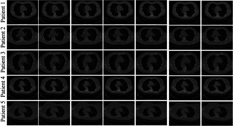
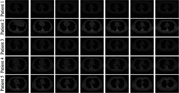
All chest CT scans were performed during a single full inspiratory breath-hold in a supine position on a 128-slice multidetector-row CT scanner (Philips Ingenuity Core, Philips Healthcare, Netherlands). No intravenous or oral contrast media were administered. The CT examinations were performed at 120 kV, 226 mAs (using automatic tube current modulation – Z-DOM, Philips), 1.08 spiral pitch factor, 0.5-s gantry rotation time, and 64*0.625 detector configurations. One-mm thick images were reconstructed with soft tissue kernel using a 512 × 512 matrix (mediastinal window) and with lung kernel using a 768 × 768 matrix (lung window). CT images were reviewed on the Picture Archiving and Communication System (PACS) workstation equipped with two 35 × 43 cm monitors produced by Eizo, with 2048 × 1536 matrix. The data comprised of 20–35 slices per patient giving 990 CT scans for Controls and 705 CT scans for COVID patients. A grid of five sample Control patients’ original grayscale lung CT scans is shown in Fig. 1, while a similar pattern for the COVID patients is shown in Fig. 2.

Fig. 1.

Five sample Control patients (representing five rows) showing original raw grayscale CT slices

Fig. 2.

Five COVID sample patients (representing five rows) original grayscale images

Baseline characteristics

The baseline characteristics of the Italian cohort’s COVID-19 data are presented in Table 1. We have utilized the MedCalc package to perform a t-test on the data, with the level of significance set to P < =0.05. The table shows the essential characteristic traits of CoP patients.

Table 1.

Baseline characteristics of CoP and NCoP patients

SN	Characteristic	Acronym	Description	CoP (N = 100)	NCoP (N = 30)	p values
1	Age (years)	–	–	50.12	51.4	0.0021
2	Gender (M)	–	–	0.685	0.68	0.0029
3	GGO	Ground Glass Opacities	An area characterized by hazy lung opacity through which vessels and bronchial structures may still be seen.	4.54	1.77	< 0.0001
4	CONS	Consolidations	A pulmonary consolidation is a region of compressible lung tissue that has filled with fluid instead of air	3.08	2.53	< 0.0001
5	PLE	Pleural Effusion	The collection of excess fluid between the layers of the pleura outside the lungs.	0.114	0.63	0.1608
6	LNF	Lymph Nodes	A kidney-shaped organ of the lymphatic system and a part of adaptive immune system.	0.171	0.20	0.0117
7	Cough	–	–	0.6	0.40	0.0029
8	Sore Throat	–	–	0.114	0.06	0.5725
9	Dyspnoea	–	Shortness of breath	0.828	0.40	0.0001

Lung CT segmentation

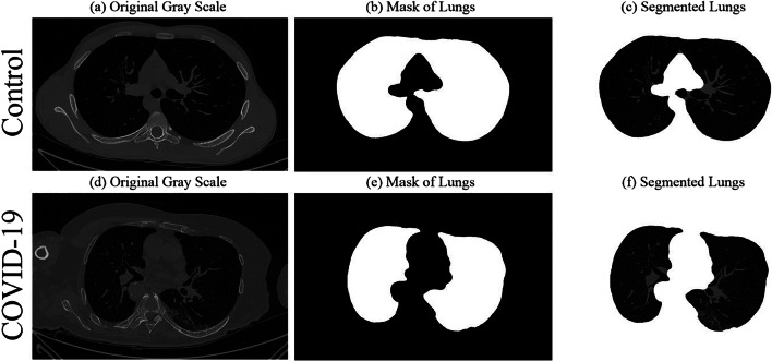
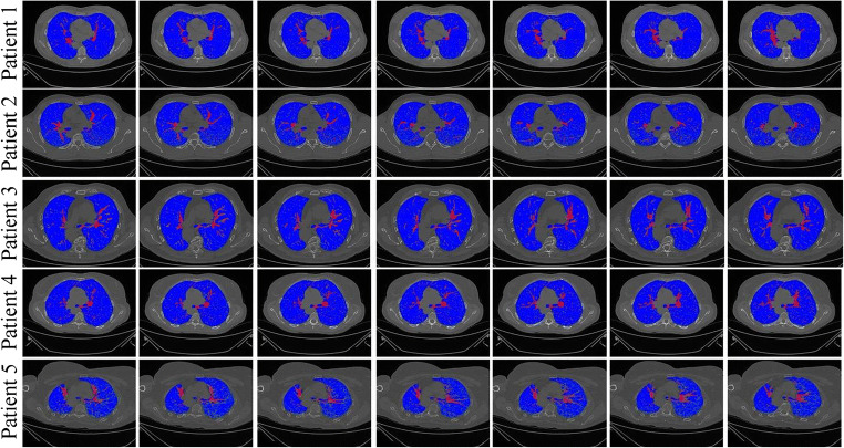
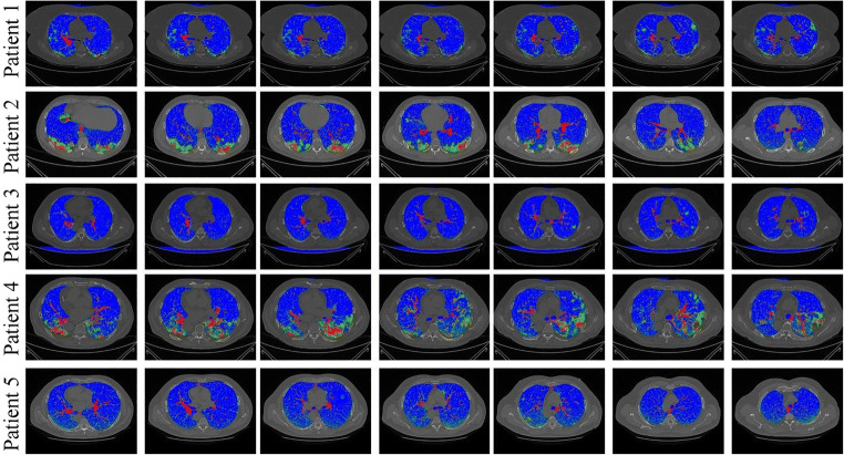
Several methods for lung CT segmentation have been developed by our group previously [11, 36, 37]. These methods were mainly for lung segmentation followed by risk stratification due to cancer. For simplicity, we used the following steps to segment the lung: (i) A lung mask creation tool was utilized from Neuroimaging Tools and resource collaboratory called “NIHLungSegmentation” tool for creating the masks of lungs in DICOM format using original DICOM CT scans. (ii) The original CT scans and masks in DICOM format were converted to PNG format using software called “XMedCon” [38]. (iii) The PNG masks were refined by using image processing closing operation to smoothen the masks. (iv) Smoothened masks were then used to segment lungs from original grayscale PNG formed in the previous step. Thus, using original CT scans, a lung mask for COVID and Control patients was generated. A sample grayscale image, its mask, and segmented lung are shown in Fig. 3. A grid of five sample Control and COVID patients’ masked lungs is shown in Figs. 4 and 5, respectively.

Fig. 3.

Sample Control patient’s a original grayscale image, b lung mask, c segmented lung; Sample COVID-19 patient’s d original grayscale image, e lung mask, f segmented lung

Fig. 4.

Five sample Control patients (shown in five rows) with colored segmented lungs

Fig. 5.

Five sample COVID patients (shown in five rows) with colored segmented lungs

Deep learning architecture

A deep-learning convolution neural network (CNN) was designed with an input convolution layer having 32 filters followed by max-pooling layer. This was adapted due to its simplicity. These were followed by another convolution layer of 16 filters followed by a max-pooling layer. In their succession was a flatten layer to convert the 2-D signal to 1-D and then another dense layer of 128 nodes. Finally, a softmax layer was present with two nodes for classification in two classes Control and COVID. The architecture of deep learning-based CNN thus has a total of 7 layers mainly adapting for simplicity. The diagrammatic view is shown in Fig. 6.

Fig. 6.

Deep learning architecture of CNN

Transfer learning architectures

Transfer learning is a mechanism to use already trained networks on a certain dataset and further calibrate them for desired needs. For example, a person knowing to ride a bicycle can use the learning and learn riding motorbike using that learning. In this study five such pre-trained networks have been used namely, VGG16, DenseNet121, DenseNet169, DenseNet201, and MobileNet. These networks have been trained on famous ImageNet dataset and by adding an extra softmax layer of two nodes at the end of the network we can make them functional for our COVID classification. The architectures of these models are shown in Appendix I (Fig. 26, 27, 28 ,29 and 30). A comparison of different DL/TL models (1 DL and 5 TL) in terms of layers is shown in Table 2.

Fig. 26.

Transfer learning architecture of VGG16

Fig. 27.

Transfer learning architecture of DenseNet121

Fig. 28.

Transfer learning architecture of DenseNet169

Fig. 29.

Transfer learning architecture of DenseNet201

Fig. 30.

Transfer learning architecture of MobileNet

Table 2.

A comparison of number of different layers in 5 TL models and 1 proposed CNN

AI Models	DL/TL	Conv2D	MaxPool	BN*	Dense	Concatenate	Activation	# Layers
CNN	DL	2	2	0	3	0	0	7
VGG16	TL	13	5	0	3	0	0	25
MobileNet	TL	27	0	27	3	0	27	88
DenseNet121	TL	120	1	121	3	58	120	432
DenseNet169	TL	168	1	169	3	82	168	600
DenseNet201	TL	200	1	201	3	98	200	712

*BN: Batch Normalization

Machine learning architecture and experimental protocols

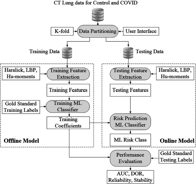
The ML-architecture for classification of COVID and Control patients is shown in Fig. 7. It consists of two parts: offline system and online system. The offline system consists of two main steps: (a) training feature extraction and (b) training classifier design to generate the offline coefficients (covered by dotted box on the left). The online system also consists of two main steps: (a) online feature extraction and (b) class prediction (Control or COVID). Such a system has been developed by our group before for tissue characterization for different applications such as liver cancer [39–41], thyroid cancer [42–44], ovarian cancer [45–47], atherosclerotic plaque characterization [48–53], and lung disease classification [37]. The classification of lungs into COVID and Control was implemented using three ML methods namely ANN, DT, and RF.

Fig. 7.

Machine learning architecture showing the offline and online system

Experimental protocol

Protocol 1: Accuracy using K-fold cross-validation protocol

Different K-fold cross-validation protocols were executed to test the accuracy of the system. K-fold cross-validation uses run time split of data into training and testing based on a split ratio and the system was trained using the training part and later tested using the testing images. The system adapted five kinds of features that were used in training and testing ML classifiers namely Haralick [39], HOG, Hu-moments [47], LBP [54, 55], and GLRLM features. The features were added one-by-one at a time to run K-fold protocols: K2, K4, K5, and K10. The following set of mean parameters was further calculated to assess the system performance as given in Eq. 1, 2, 3, and 4.

$$\overline{A}\left(\mathrm{c}\right)=\frac{\sum _{\mathrm{f}}^{\mathrm{F}}\sum _k^{\mathrm{K}}\sum _i^{{\mathrm{C}}_{\mathrm{o}}}A\left(\mathrm{c},\mathrm{f},\mathrm{k},\mathrm{i}\right)}{F\times K\times C_o}$$ 1

Where, Ᾱ(c)is the accuracy for a classifier for a set of features (f) and different K-fold cross-validation protocols (k) and a combination number of K-fold protocol (i).

$$\overline{A}\left(\mathrm{f}\right)=\frac{\sum _{\mathrm{c}}^{{\mathrm{C}}_{\mathrm{l}}}\sum _k^{\mathrm{K}}\sum _i^{{\mathrm{C}}_{\mathrm{o}}}A\left(\mathrm{c},\mathrm{f},\mathrm{k},\mathrm{i}\right)}{C_l\times K\times C_o}$$ 2

Where Ᾱ(f)is the accuracy for a feature for a set of classifiers (c) and different K-fold cross-validation protocols (k) and the combination number of K-fold protocol (i).

$$\overline{A}\left(\mathrm{k}\right)=\frac{\sum _{\mathrm{c}}^{{\mathrm{C}}_{\mathrm{l}}}\sum _{\mathrm{f}}^{\mathrm{F}}\sum _i^{{\mathrm{C}}_{\mathrm{o}}}A\left(\mathrm{c},\mathrm{f},\mathrm{k},\mathrm{i}\right)}{C_l\times F\times C_o}$$ 3

Where Ᾱ(k)is the accuracy for any K-fold protocol for a set of classifiers (c) and different features (f) and the combination number of K-fold protocol (i).

$${\overline{A}}_{\mathrm{sys}}=\frac{\sum _{\mathrm{c}}^{{\mathrm{C}}_{\mathrm{l}}}\sum _{\mathrm{f}}^{\mathrm{F}}\sum _k^{\mathrm{K}}\sum _i^{{\mathrm{C}}_{\mathrm{o}}}A\left(\mathrm{c},\mathrm{f},\mathrm{k},\mathrm{i}\right)}{C_l\times F\times K\times C_o}$$ 4

Where Ᾱ_sys is the system mean accuracy for any set of classifiers (c), features (f), K-fold protocols (k), and combination number (i) C_l is the number of classifiers equal to 3, F is the feature set equal to 3, K is the number of partition protocols equal to 4 and C_o is the number of combinations for a particular K-fold protocol. The symbol A is used for accuracy in Eqs. (1)–(4). The results were analyzed based on (a) accuracy, (b) area under the curve (AUC) and (c) diagnostics odds ratio (DOR), which will be discussed in performance evaluation section.

Results

DL and TL classification results

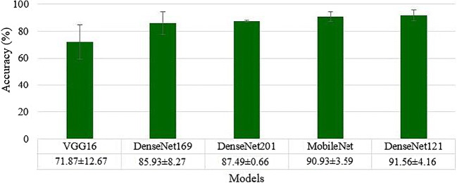
The deep learning architecture as explained in section 3.3 was used for classification of Control vs. COVID. The K10 cross-validation protocol was used that gave the accuracy of 99.41 ± 5.12%, with an AUC of 0.991 (p < 0.0001). We used five transfer learning methods namely VGG16, DenseNet121, DenseNet169, DenseNet201 and MobileNet as described in section 3.4. The best accuracy was obtained by DenseNet121: 91.56 ± 4.16% with an AUC of 0.913, p < 0.0001, followed by MobileNet: 90.93 ± 3.59%, with an AUC of 0.893, p < 0.0001, DenseNet201: 87.49 ± 0.66%, with an AUC of 0.871, p < 0.0001, DenseNet169: 85.93 ± 8.27%, with an AUC of 0.852, p < 0.0001, and VGG16: 71.87 ± 12.67%, with an AUC of 0.714, p < 0.0001. These results were obtained using the K10 cross-validation protocol. A plot of mean accuracy along with their standard deviations of five transfer learning models is shown in Fig. 8.

Fig. 8.

Mean accuracies of five different transfer learning models

ML classification results

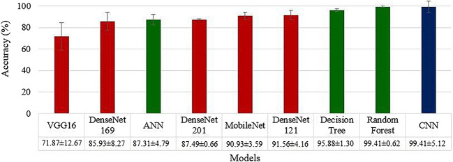
As detailed in section 3.5, three ML classifiers ANN, DT and RF were executed on the entire dataset using five features (i) LBP, (ii) Haralick, (iii) Histogram of oriented gradients (HOG), (iv) Hu-moments and (v) Gray Level Run Length Matrix (GLRLM). These 5 × 3 sets of feature combinations and classifiers were executed for four K-fold cross-validation protocols (K2, K4, K5, and K10) and mean accuracy was calculated for each combination with a K-fold protocol. The best K10 mean accuracy was noticed for the Random Forest model by including all the five features leading to 99.41 ± 0.62%, having an AUC of 0.988, (p < 0.0001) followed by DT including all the five features: 95.88 ± 1.30%, 0.948 (p < 0.0001). The accuracy of ANN was also best with all five features, 87.31 ± 4.79%, 0.861 (p < 0.0001). A comparison plot of ML, TL and DL accuracies is given in Fig. 9.

Fig. 9.

Comparison of 9 AI models with increasing order of classification accuracies. ML methods shown in green, TL methods are shown in red, and DL method shown in blue. K10 protocol was executed for these accuracies

Mean accuracies of 3 ML classifiers based on Eqs. (1–4) are shown in Appendix II (Fig. 31, 32, 33 and 34).

Fig. 31.

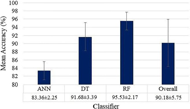
Mean accuracies of three different ML (ANN, DT, RF) based classifiers

Fig. 32.

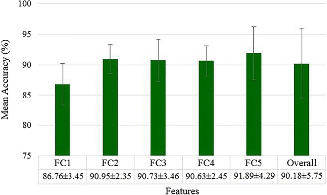
Mean accuracies over all ML classifier for different features (FC1 to FC5)

Fig. 33.

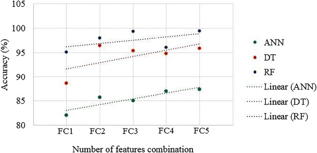
Effect of feature addition on classification accuracy for ML classifiers

Fig. 34.

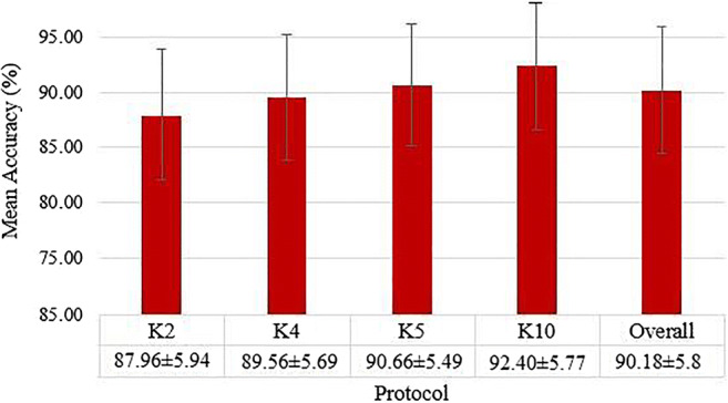
Mean accuracies over all the classifiers and all the features for different K-fold protocols using ML models

COVID separation index

COVID Separation Index (CSI) is mathematically defined as:

$$\mathrm{CSI}=\left(\frac{\left|{\mathrm{\mu }}_{\text{COVID}}-{\mathrm{\mu }}_{\text{Control}}\right|}{{\mathrm{\mu }}_{\text{Control}}}\right)\times 100$$ 5

where μ_COVID is the mean feature value for COVID block and μ_Control is the mean feature value for Control blocks. CSI for the different set of features is shown in Table 3. As seen in Table 3 all the features have similar CSI in range 35–50. If these values are high, this reflects the changes of higher classification accuracy.

Table 3.

CSI for the different set of features

	C1	C2	C3	C4
	Features	Feature Strength (Control)	Feature Strength (COVID)	CSI
FC1	LBP	0.03956 ± 0.0023	0.05555 ± 0.0027	40.41962
FC2	LBP + Haralick	928.46 ± 35.45	1395.27 ± 57.46	50.27788
FC3	LBP + Haralick+HOG	1.8734 ± 0.34	1.2075 ± 0.17	35.545
FC4	Haralick+LBP + HOG+Hu-moments	1.873 ± 0.28	1.207 ± 0.16	35.55793
FC5	Haralick+LBP + HOG+Hu-moments+GLRLM	3.1586 ± 0.76	1.9536 ± 0.54	38.14981

C Column, R Row.

Tissue characterization of COVID-19 disease

Spatial gridding process

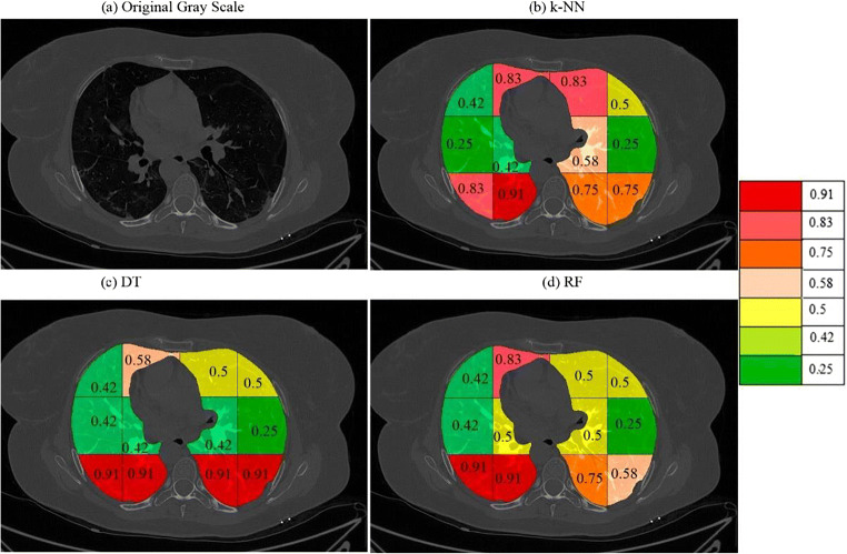
Lungs infected due to SARS-CoV-2 shows regions of hyperintensity in certain regions. An effort was thus made to identify the lung region which was most affected. The segmented lungs were divided into 12 blocks consisting of 3 rows each having 4 blocks, spanning left and right lungs. The pictorial representation of this grid on the segmented lungs for the sample Control and COVID patient is shown in Fig. 10.

Fig. 10.

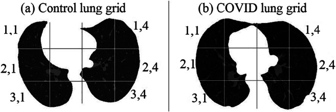
Division of segmented lungs into 12 blocks of a Control and b COVID patient

Stacking concept mutually exclusive for each block

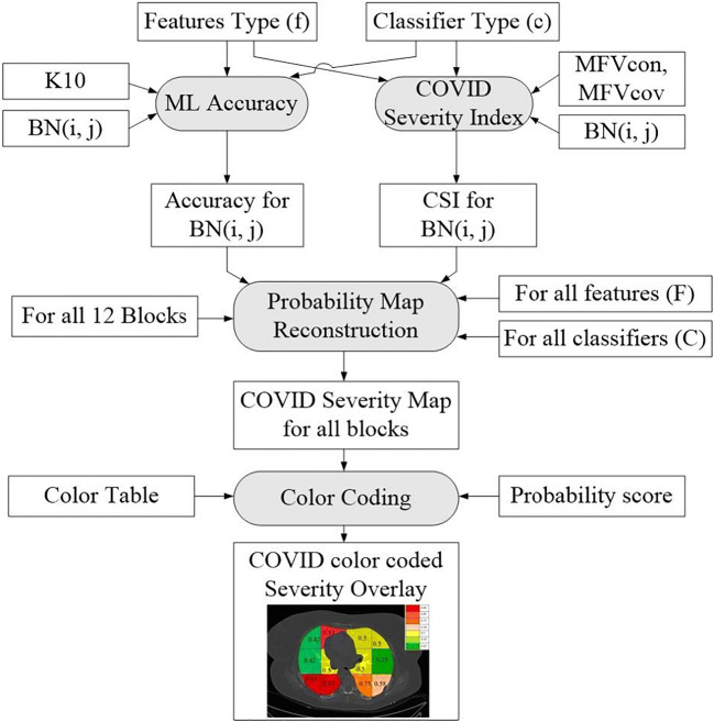
Figure 11 shows a conceptual stack of all blocks of a particular location of the grid (say for (3,1) shown in Fig. 20) for Control and COVID patients which is used to calculate K10 classification accuracy and CSI values. These values are used to calculate block score and finally its severity value in the form of a probability. Since there are 12 blocks in the grid, there will be 12 such vectors each corresponding to that grid location. This vector will be the stack of all the patients for Control and COVID combination, which will be used for feature extraction.

Fig. 11.

Process flow of calculating the probability of COVID severity for each blocks (Courtesy of AtheroPoint™, CA, USA)

Fig. 20.

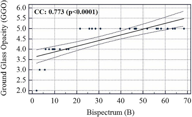
Association between Bispectrum and GGO values

Scoring concept for each block and its probability computation

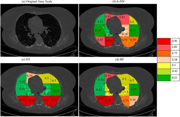
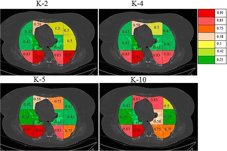
Given the ML accuracy and CSI values, one then computes the score for each block corresponding to the feature selected (f) and classifier selected (c). Points are assigned to each block depending upon the location in the 2 × 2 quadrant of the “classification accuracy vs. COVID separation index” plot. This is shown in Fig. 12, where values are assigned to each quadrant ranging from 1 to 4. The block values are then assigned colors depending upon the probability computed. Color changes are assigned from red, pink, orange, cream, yellow, light green, dark green as per the probability maps per block.

Fig. 12.

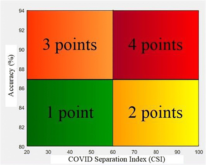
The division of classification accuracy vs. COVID separation index graph into 4 quadrants and points for each quadrant

Overall architecture of the block imaging system

The overall system architecture of the Block imaging system for COVID severity computation is shown in Fig. 13. The two main blocks are (a) the probability map computation and (b) color coding. Note that, since there are four partition protocols, three sets of features, three set of classifiers, and a set of 12 blocks for Block imaging, therefore, there are 4× 12× 3× 3 (432) block points. Thus, for each combination of training protocol “k” and each set of classifier “c”, we get a probability map. Therefore, there will be 4 × 3 = 12 probability maps. Technically we get 36 block points for each combination of “k, c”.

Fig. 13.

Architecture design of the Block Imaging strategy for COVID disease characterization

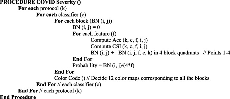
COVID severity computation algorithm

These individual blocks were passed through K-fold protocols to find the accuracy and COVID separation index (CSI) for all features and classifiers combinations. Based on these values a severity probability is calculated for each block and color code is given to each probability starting from red with the highest probability and green lowest. This type of graph was created for all 3 classifiers and the graph was divided into 4 quadrants with points being given to a block depending on the quadrant they lie.

The pseudo code for the block severity is shown as follows:

Results of accuracy vs. CSI computation on different blocks

The entire database of Controls and COVID was segmented into lung blocks and each block was analyzed in terms of K10 accuracy of RF, DT, and k-NN classifiers. Each block mean features were also calculated and the COVID separation index (CSI) was calculated for different sets of features using Eq. 5. The sets of features used were: Haralick with LBP, Hu-moments with Haralick and LBP with Hu-moments. A graph of accuracy vs. CSI was plotted for each classifier with one of 3 sets of features as shown in Fig. 14.

Fig. 14.

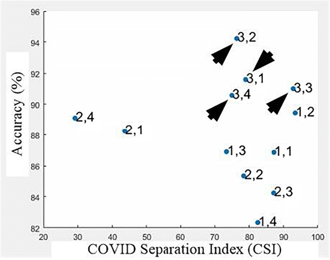
A plot of accuracy vs. CSI using RF classifier with Hu-moments and Haralick features for all blocks

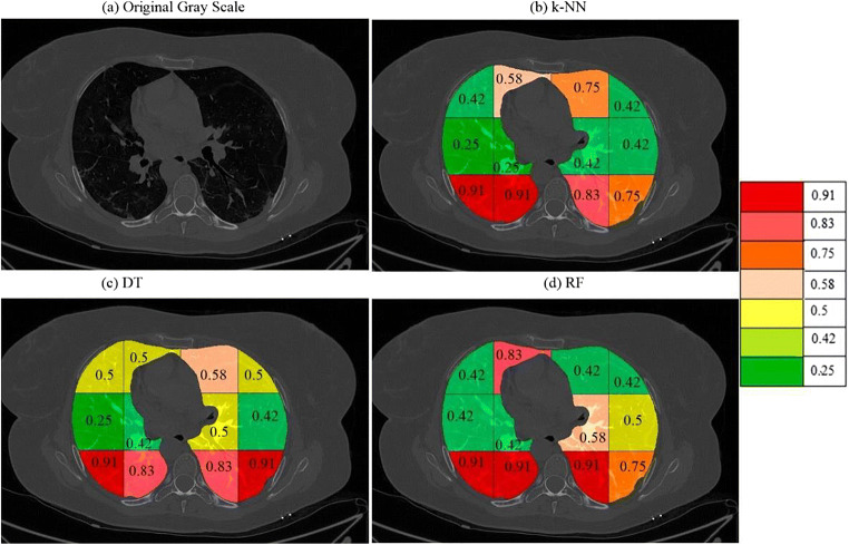
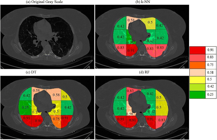
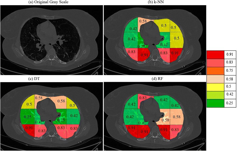
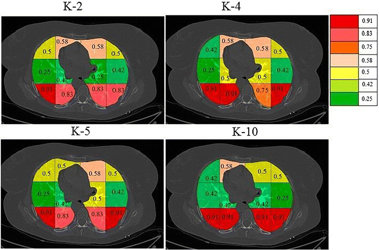
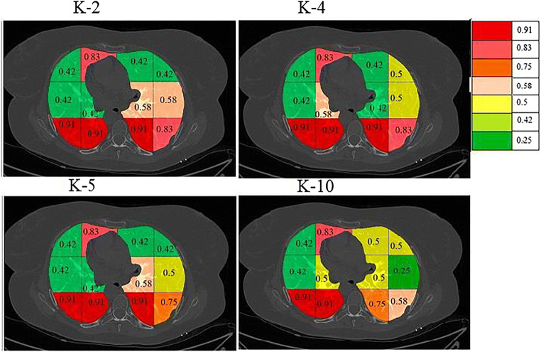
On giving points to each block in this way the final probabilities were calculated independently for each classifier and a color code was given to each block. The block with the highest probability was given a bright red color and then orange and then yellow and then green. The points and probability of each block for RF are given in Table 4. A sample diseased patient color-coded image for k-NN, DT, and RF is shown in Fig. 15. These clearly show that maximum COVID severity is in lower right lung regions. More figures of color-coded images for different classifiers and protocols are given in Appendix III (Fig. 35, 36, 37, 38, 40 and 41). The mean probability values for all blocks for different partition protocols are given in Appendix III (Table 10) and for different classifiers are given in Appendix III (Table 11).

Table 4.

Points to each block and combined probability of each block

	C1	C2	C3	C4	C5
	Random Forest
	Block	Haralick + LBP	Haralick + Hu moments	LBP + Hu moments	Probability (RF)
R1	1,1	2	2	1	0.42
R2	1,2	4	4	2	0.83
R3	1,3	2	2	2	0.5
R4	1,4	2	2	2	0.5
R5	2,1	3	1	1	0.42
R6	2,2	3	2	1	0.5
R7	2,3	3	2	1	0.5
R8	2,4	1	1	1	0.25
R9	3,1	4	4	3	0.92
R10	3,2	4	4	3	0.92
R11	3,3	4	4	1	0.75
R12	3,4	2	4	1	0.58

Fig. 15.

a A sample grayscale diseased image, Color-coded blocks of diseased lung using b k-NN, c DT, and d RF

Fig. 35.

a A sample grayscale diseased image, Color coded blocks of COVID lung using K10 protocol for b k-NN, c DT, and d RF classifiers

Fig. 36.

a A sample grayscale diseased image, Color coded blocks of COVID lung using K5 protocol for b k-NN, c DT, and d RF classifiers

Fig. 37.

a A sample grayscale diseased image, Color coded blocks of COVID lung using K4 protocol for b k-NN, c DT, and d RF classifiers

Fig. 38.

a A sample grayscale diseased image, Color coded blocks of COVID lung using K2 protocol for b k-NN, c DT, and d RF classifiers

Fig. 40.

A sample COVID patient’s image with color coded blocks of COVID lung using DT classifier for a K2 b K4, c K5, and d K10 protocols

Fig. 41.

A sample COVID patient’s image with color coded blocks of COVID lung using RF classifier for a K2 b K4, c K5, and d K10 protocols

Table 10.

Training protocol-wise probability maps for different four different classifiers

Block	K10			Mean	K5			Mean	K4			K2			Mean	Overall Mean
	RF	DT	kNN		RF	DT	kNN		RF	kNN	Mean	RF	DT	kNN
1,1	0.42	0.42	0.42	0.42	0.42	0.5	0.42	0.45	0.42	0.42	0.42	0.42	0.5	0.42	0.45	0.44
1,2	0.83	0.67	0.83	0.78	0.75	0.5	0.58	0.61	0.83	0.58	0.66	0.83	0.58	0.58	0.66	0.68
1,3	0.5	0.5	0.83	0.61	0.42	0.58	0.75	0.58	0.42	0.5	0.5	0.42	0.58	0.5	0.5	0.55
1,4	0.5	0.5	0.5	0.5	0.42	0.5	0.42	0.45	0.5	0.42	0.47	0.42	0.5	0.5	0.47	0.47
2,1	0.42	0.42	0.25	0.36	0.42	0.25	0.25	0.31	0.42	0.42	0.36	0.42	0.25	0.42	0.36	0.35
2,2	0.5	0.42	0.42	0.45	0.42	0.42	0.25	0.36	0.58	0.25	0.44	0.42	0.42	0.25	0.36	0.4
2,3	0.5	0.42	0.58	0.5	0.58	0.5	0.42	0.5	0.42	0.42	0.45	0.58	0.25	0.42	0.42	0.47
2,4	0.25	0.25	0.25	0.25	0.5	0.42	0.42	0.45	0.5	0.42	0.45	0.58	0.42	0.5	0.5	0.41
3,1	0.92	0.92	0.83	0.89	0.92	0.92	0.92	0.92	0.92	0.83	0.89	0.92	0.92	0.83	0.89	0.9
3,2	0.92	0.92	0.92	0.92	0.92	0.83	0.92	0.89	0.92	0.92	0.92	0.92	0.83	0.92	0.89	0.91
3,3	0.75	0.92	0.75	0.81	0.92	0.83	0.83	0.86	0.92	0.83	0.83	0.92	0.83	0.83	0.86	0.84
3,4	0.58	0.92	0.75	0.75	0.75	0.92	0.75	0.81	0.83	0.83	0.86	0.83	0.83	0.92	0.86	0.82

Table 11.

Classifier-wise probability map for four training protocols using three kinds of classifiers

Block	k-NN				Mean	DT				Mean	RF				Mean	Overall Mean
	K2	K4	K5	K10		K2	K4	K5	K10		K2	K4	K5	K10
1,1	0.42	0.42	0.42	0.42	0.42	0.5	0.42	0.5	0.42	0.46	0.42	0.42	0.42	0.42	0.42	0.43
1,2	0.58	0.58	0.58	0.83	0.64	0.58	0.58	0.5	0.67	0.58	0.83	0.83	0.75	0.83	0.81	0.68
1,3	0.5	0.5	0.75	0.83	0.65	0.58	0.58	0.58	0.5	0.56	0.42	0.42	0.42	0.5	0.44	0.55
1,4	0.5	0.42	0.42	0.5	0.46	0.5	0.5	0.5	0.5	0.5	0.42	0.5	0.42	0.5	0.46	0.47
2,1	0.42	0.42	0.25	0.25	0.34	0.25	0.25	0.25	0.42	0.29	0.42	0.42	0.42	0.42	0.42	0.35
2,2	0.25	0.25	0.25	0.42	0.29	0.42	0.5	0.42	0.42	0.44	0.42	0.58	0.42	0.5	0.48	0.4
2,3	0.42	0.42	0.42	0.58	0.46	0.25	0.5	0.5	0.42	0.42	0.58	0.42	58	0.5	0.52	0.47
2,4	0.5	0.42	0.42	0.25	0.4	0.42	0.42	0.42	0.25	0.38	0.58	0.5	0.5	0.25	0.46	0.41
3,1	0.83	0.83	0.92	0.83	0.85	0.92	0.92	0.92	0.92	0.92	0.92	0.92	0.92	0.92	0.92	0.9
3,2	0.92	0.92	0.92	0.92	0.92	0.83	0.92	0.83	0.92	0.88	0.92	0.92	0.92	0.92	0.92	0.91
3,3	0.83	0.83	0.83	0.75	0.81	0.83	0.75	0.92	0.92	0.83	0.92	0.92	0.92	0.75	0.88	0.84
3,4	0.92	0.83	0.75	0.75	0.81	0.83	0.92	0.92	0.92	0.9	0.83	0.83	0.75	0.58	0.75	082

Characterization method-II: Bispectrum analysis

The Bispectrum is a useful measure of the Higher-Order spectrum (HOS) for analyzing the non-linearity of a signal. Several applications of HOS have been published by our group for tissue characterization [44, 56–59].

COVID lungs have an extra white congestion area these pixels were separated and passed to Radon transform which was used as a signal for higher-order spectrum (HOS) based Bisprectrum (B) calculation. The Bispectrum are powerful tools to detect the non-linearity in the input signal [60, 61]. Radon transform becomes highly nonlinear when there is a sudden change in grayscale image density. Thus, COVID images are characterized with the help of higher B values. The equation for Bispectrum is as given in Eq. 6.

$$\text{Bispectrum}\left(\mathbf{B}\left(\mathrm{f}1,\mathrm{f}2\right)\right)=\mathrm{E}\left[\mathcal{F}\left(\mathrm{f}1\right)\times \mathcal{F}\left(\mathrm{f}2\right)\times \mathcal{F}\left(\mathrm{f}1+\mathrm{f}2\right)\right]$$ 6

where, B is the Bispectrum value, $\mathcal{F}$ is the Fourier transforms and E is the expectation operator. The region Ω of computation of bispectrum and bispectral features of a real signal is uniquely given by a triangle 0 < = f2 < = f1 < = f1 + f2 < = 1.

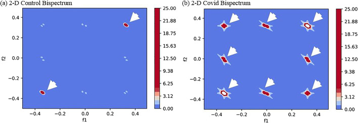
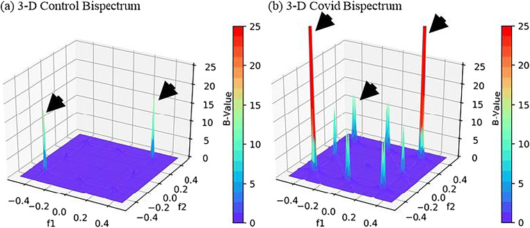
The images were found to have more diseased pixels in the range 20–40 intensity thus a radon transform of these pixels were taken to transform an image in the form of a signal which was passed to Bispectrum function and 2-D and 3-D plots were created for Control and COVID classes. As expected, the B-values for COVID class were much higher due to several diseased pixels in these images. The 2-D and 3-D plots of Bispectrum for two classes are shown in Figs. 16 and 17.

Fig. 16.

Comparison of Bispectrum 2-D plots for a Control and b COVID class

Fig. 17.

Comparison of Bispectrum 3-D plots for a Control and b COVID class

Characterization method-III: Block entropy

As explained in section 6.1 the lungs were divided into 12 blocks using a grid. The same blocks were used to compute the entropy of each block for Controls and COVID. This process was used to show that there is greater chaotic (or randomness) in certain parts of diseased lungs due to the presence of white regions of congestion. The equation for entropy is as given in Eq. 7.

$$\text{Entropy}=-{\sum }_{\mathrm{i}=0}^{\mathrm{N}}{\mathrm{p}}_{\mathrm{i}}log\left({\mathrm{p}}_{\mathrm{i}}\right)$$ 7

Where p_i is the probability of any pixel intensity i in the input image and N is the total number of intensity levels in the grayscale image equal to 255. Entropy is a useful measure of showing the texture of images [37, 44, 60]. If the image has more roughness then it will have higher entropy [47, 62]. The entropy was calculated for each block as shown in Fig. 12. A plot was made for entropies of blocks of Control and COVID class as shown in Fig. 18. As seen the entropy of blocks of lower regions of lungs is higher than Control due to disease regions more prominent in the lower part of the lungs. The percentage increase in entropy for the COVID class is shown in Table 5.

Fig. 18.

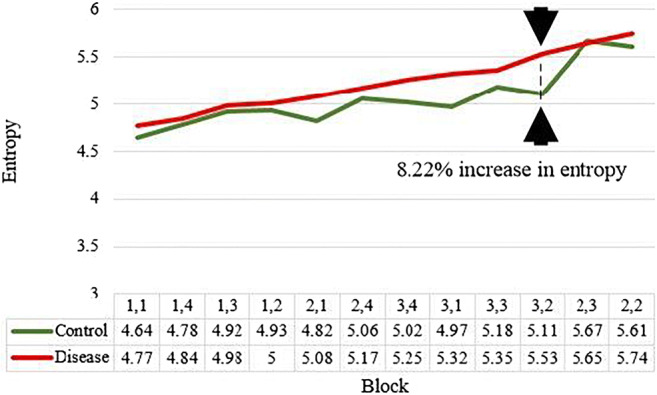
Comparison of block-wise entropy for Control and COVID disease classes

Table 5.

The percent gain in entropy of disease lung shows higher values in the lower part of the lungs

	C1	C2	C3	C4
		Control	Disease	% Gain
R1	1,1	4.64	4.77	2.80
R2	1,4	4.78	4.84	1.25
R3	1,3	4.92	4.98	1.21
R4	1,2	4.93	5	1.41
R5	2,1	4.82	5.08	5.39
R6	2,4	5.06	5.17	2.17
R7	3,4	5.02	5.25	4.58
R8	3,1	4.97	5.32	7.04
R9	3,3	5.18	5.35	3.28
R10	3,2	5.11	5.53	8.21
R11	2,3	5.67	5.65	0.35
R12	2,2	5.61	5.74	2.31

Validation of block imaging

The COVID severity was computed for each block in the grid and a mean was taken for all the blocks to find the overall COVID severity of a patient. All the slices of a particular patient were fed to an ML system trained on all patients except that patient and using Block Imaging algorithm described above its block-wise severity was calculated. Further, the mean of all blocks was computed. Evaluating in this fashion and comparing it with Ground Glass Opacity (GGO) values of CT scans of all patients it was found that the two series had a correlation coefficient of 0.9145 (p < 0.0001). Similarly, correlation of COVID severity with Bispectrum values (Bispectrum is explained in next section 5.2) for each patient was found to be 0.66 (p = 0.0001). The list of all patients COVID severity, Bispectrum strength, CONS (A pulmonary consolidation is a region of compressible lung tissue that has filled with fluid instead of air), and GGO values are shown in Table 12 (Appendix IV). The correlation and p values between variables of Table 12 (Appendix IV) are given in Table 6. The association between GGO and COVID severity is shown in Fig. 19, between GGO and Bispectrum strength is given in Fig. 20, and between COVID severity and Bispectrum strength is shown in Fig. 21. As seen the correlation between COVID severity and GGO values is quite high and similarly correlation between COVID severity and Bispectrum strength is also strong and further validates the COVID severity values.

Table 12.

The COVID severity values as compared to GGO values

	R1	R2	R3	R4	R5	R6
	Patient Number	GGO	CONS	LNF	Bispectrum strength	COVID Severity
C1	1	5	2	0	46.59	0.821
C2	2	4	0	0	6.03	0.782
C3	3	4	1	0	7.48	0.792
C4	4	5	5	0	46.67	0.825
C5	5	4	2	1	9.03	0.775
C6	6	4	3	0	9.46	0.749
C7	7	5	1	0	39.71	0.833
C8	8	4	1	0	10.01	0.764
C9	9	5	5	1	21.47	0.873
C10	10	5	5	0	25.72	0.842
C11	11	5	3	1	26.91	0.833
C12	12	5	3	0	28.47	0.846
C13	13	5	5	0	30.70	0.831
C14	14	5	5	1	58.07	0.856
C15	15	5	2	0	43.87	0.823
C16	16	5	1	0	46.11	0.862
C17	17	4	4	1	12.36	0.743
C18	18	5	5	0	46.92	0.817
C19	19	5	5	0	56.01	0.831
C20	20	2	5	0	1.88	0.627
C21	21	3	0	0	3.28	0.715
C22	22	5	4	0	68.39	0.840
C23	23	4	2	0	15.30	0.770
C24	24	5	3	0	51.76	0.773
C25	25	5	2	0	61.00	0.787
C26	26	5	5	1	56.65	0.854
C27	27	5	4	0	64.34	0.884
C28	28	3	3	0	5.649	0.701
C29	29	4	3	0	16.30	0.768
C30	30	5	2	0	63.34	0.814

Table 6.

The correlation between GGO, CONS, COVID severity and Bispectrum

	GGO	CONS	LNF	Bispectrum
COVID Severity	0.9146 (p < 0.0001)	0.220 (p = 0.2407)	0.19248 (p = 0.3082)	0.6656 (p = 0.0001)
Bispectrum	0.7736 (p < 0.0001)	0.3131 (p = 0.0920)	−0.0443 (p = 0.8162)

Fig. 19.

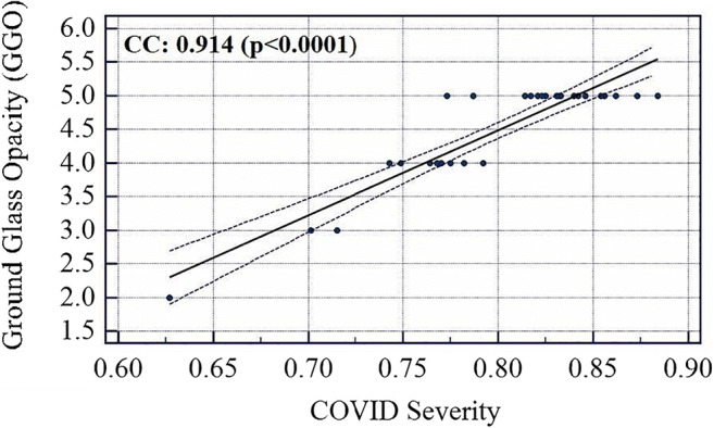
Association between COVID severity and GGO values

Fig. 21.

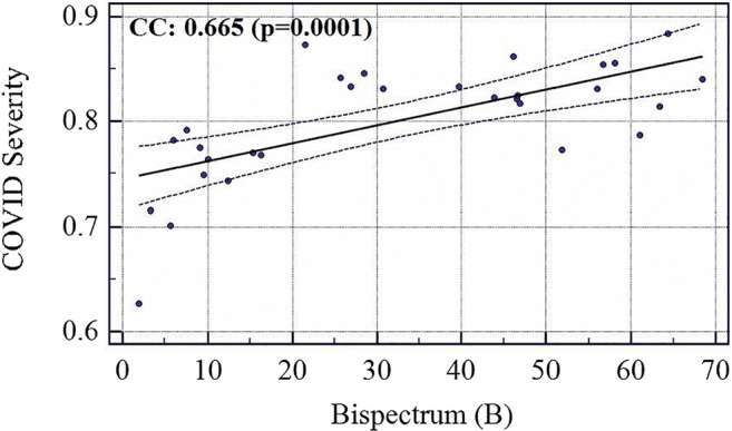
Association between Bispectrum and COVID Severity

Performance evaluation

Diagnostics odds ratio

Diagnostic Odds Ratio (DOR) is used to discriminate subjects with a target disorder from subjects without it. DOR is calculated according to Eq. 8. DOR can take any value from 0 to infinity. A test with a more positive value means better test performance. A test with value 1 means it gives no information about the disease and with a value of less than 1 means it is in the wrong direction and predicts the opposite outcomes.

$$\mathrm{DOR}=\frac{\mathrm{TP}/\mathrm{FN}}{\mathrm{FP}/\mathrm{TN}}=\frac{S_p\times S_e}{\left(1-{\mathrm{S}}_{\mathrm{p}}\right)\times \left(1-{\mathrm{S}}_{\mathrm{e}}\right)}$$ 8

Where S_e refers to the sensitivity and S_p refers to the specificity and is calculated using Eq. 9 and 10.

$$\text{Sensitivity}=\frac{\mathrm{TP}}{\mathrm{TP}+\mathrm{FN}}$$ 9

$$\text{Specificity}=\frac{\mathrm{TN}}{\mathrm{TN}+\mathrm{FP}}$$ 10

where, TP, FP, TN, and FN represent true positive, false positive, true negative, false negative. The DOR values for all ML and TL methods are shown in Table 7. The variation of accuracy and DOR for three ML classifiers and five TL methods are shown in Fig. 22.

Table 7.

Sensitivity, specificity with increasing order of DOR for the 3 ML and 5 TL systems

–	–	C1	C2	C3
–	Model	Specificity (%)	Sensitivity (%)	DOR
R1	VGG16	63.09	80.23	6.93
R2	DenseNet169	81.08	89.58	36.85
R3	ANN	81.57	91.48	47.60
R4	DenseNet201	82.66	91.57	65.00
R5	MobileNet	86.48	93.75	96.00
R6	DenseNet121	88.88	93.87	122.66
R7	DT	94.36	96.96	536.00
R8	RF	98.57	99.00	6831.00
R9	CNN	98.57	99.00	6831.00

Fig. 22.

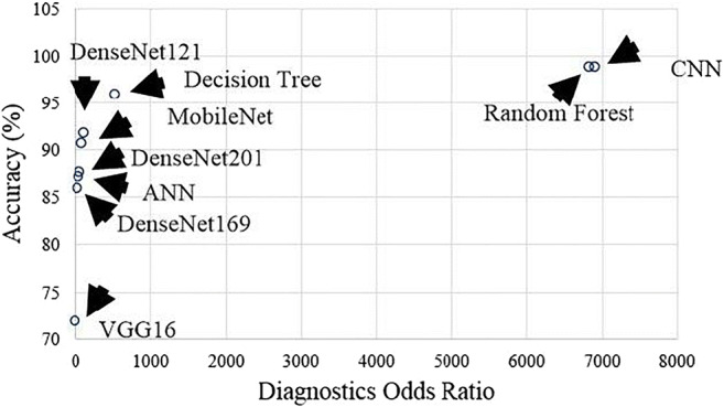
Plot showing the relation between accuracy and DOR for 3 ML and 5 TL systems

Receiver operating characteristics curve

Receiver Operating Characteristics curve shows the relationship between the false-positive rate (FPR) and the true-positive rate (TPR). The AUC validates our hypothesis. The ROC curves for 3 ML classifiers and 5 TL methods and 1 DL are given in Fig. 23. ROC curve is a plot between TPR (y-axis) and FPR (x-axis). The equation for TPR and FPR is given as Eq. 11 and 12.

$$\mathrm{TPR}=\frac{\mathrm{TP}}{\mathrm{TP}+\mathrm{FN}}$$ 11

$$\mathrm{FPR}=\frac{\mathrm{FP}}{\mathrm{FP}+\mathrm{TN}}$$ 12

Fig. 23.

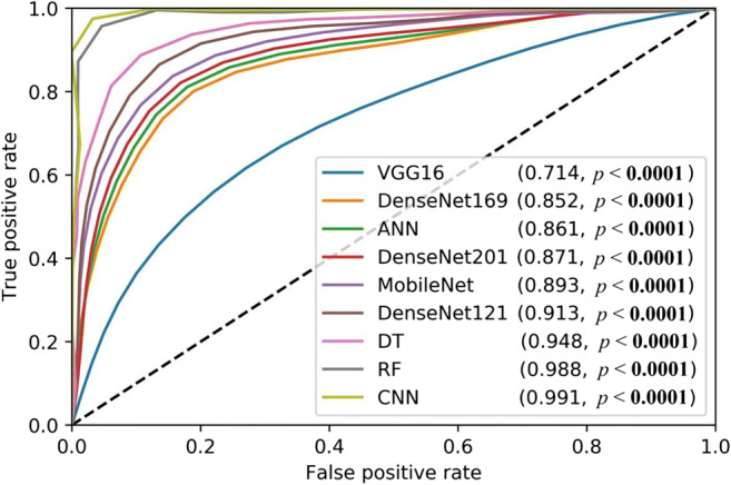
Plot showing ROC for 3 ML and 5 TL systems

Performance evaluation metrics

Various performance evaluation metrics such as specificity, sensitivity, precision, recall, accuracy, F1-score, DOR, AUC and cohen kappa score of all ML and TL classifiers are presented in Table 8 in increasing order of accuracy.

Table 8.

Performance evaluation metrics for all proposed AI methods

		C1	C2	C3	C4	C5	C6	C7	C8	C9
		Sp	Se	Precision	Recall	Acc (%)	F1-Score	DOR	AUC*	Kappa
R1	VGG16	0.630	0.802	0.69	0.80	71.87	0.741	6.93	0.714	0.434
R2	DenseNet169	0.810	0.895	0.86	0.89	85.93	0.877	36.85	0.852	0.711
R3	ANN	0.815	0.914	0.86	0.914	87.058	0.88	47.60	0.861	0.736
R4	DenseNet201	0.835	0.907	0.88	0.90	87.49	0.893	49.70	0.871	0.747
R5	MobileNet	0.864	0.937	0.9	0.93	90.93	0.918	96.00	0.893	0.807
R6	DenseNet121	0.888	0.938	0.92	0.93	91.56	0.929	122.67	0.913	0.831
R7	DT	0.943	0.969	0.96	0.969	95.882	0.964	536	0.948	0.915
R8	RF	0.985	0.99	0.99	0.99	99.41	0.99	6831	0.988	0.976
R9	CNN	0.985	0.99	0.99	0.99	99.41	0.99	6831	0.991	0.976

*all p values <0.0001

Other statistical tests like Mann Whitney and paired -tests are described in Appendix V in Tables 13, 14, 15, 16 and 17.

Table 13.

Labels are given to different feature set combinations of ML

Label	Features set combination
FC1	LBP
FC2	LBP + Haralick
FC3	LBP + Haralick+HOG
FC4	Haralick+LBP + HOG+Hu-moments
FC5	Haralick+LBP + HOG+Hu-moments+GLRLM

Table 14.

Mann Whitney tests result for the different feature set combinations of ML

	z score	p value	Mann Whitney U
FC1 versus FC2	1.091	0.2752	2
FC1 versus FC3	1.091	0.2752	2
FC1 versus FC4	0.655	0.5127	3
FC1 versus FC5	1.091	0.2752	2
FC2 versus FC3	0.218	0.8273	4
FC2 versus FC4	0.000	1.000	4.5
FC2 versus FC5	0.218	0.8273	4
FC3 versus FC4	0.218	0.8273	4
FC3 versus FC5	0.655	0.5127	3
FC4 versus FC5	0.655	0.5127	3

Table 15.

Paired t-tests results for 10 combinations of K10 protocol for TL and ML classifiers

Set of Classifiers	t value	p value	Degrees of Freedom
DenseNet121-ANN	−1.356	0.2081	9
DenseNet121-DT	3.356	0.0084	9
DenseNet121-RF	5.892	0.0002	9
MobileNet-ANN	−0.873	0.4053	9
MobileNet-DT	3.582	0.0059	9
MobileNet-RF	6.624	0.0001	9
DenseNet201-ANN	2.001	0.0764	9
DenseNet201-DT	5.702	0.0003	9
DenseNet201-RF	7.857	< 0.0001	9
DenseNet169-ANN	1.354	0.2088	9
DenseNet169-DT	3.644	0.0054	9
DenseNet169-RF	5.029	0.0007	9
VGG16-ANN	4.58	0.0013	9
VGG16-DT	5.764	0.0003	9

Table 16.

Paired t-tests results for 10 combinations of K10 protocol for DL and ML classifiers

Set of Classifiers	t value	p value	Degrees of Freedom
CNN-ANN	−17.954	<0.0001	9
CNN-DT	−7.076	0.0001	9
CNN-RF	0.00135	0.999	9

Table 17.

Paired t-tests results for 10 combinations of K10 protocol for DL and TL classifiers

Set of Classifiers	t value	p value	Degrees of Freedom
CNN-DenseNet121	−5.642	0.0003	9
CNN-MobileNet	−7.054	0.0001	9
CNN-DenseNet201	−8.832	<0.0001	9
CNN-DenseNet169	−5.321	0.0005	9
CNN-VGG16	−6.786	0.0001	9

Power analysis

We follow the standardized protocol for estimating the total samples needed for a certain threshold of the margin of error. The standardized protocol consisted of choosing the right parameters while applying the “power analysis” [63–66]. Adapting the margin of error (MoE) to be 3%, the confidence interval (CI) to be 97%, the resultant sample size (n) was computed using the following equation:

$$\mathrm{n}=\left[{\left({\mathrm{z}}^{\ast }\right)}^2\times \left(\frac{\widehat{\mathrm{p}}\left(1-\widehat{\mathrm{p}}\right)}{{\mathrm{MoE}}^2}\right)\right]$$ 13

where z∗ represents the z-score value (2.17) from the table of probabilities of the standard normal distribution for the desired CI, and p̂ represents the data proportion (705/(705 + 990) = 0.41). Plugging in the values, we obtain the number of samples 1265 (as a baseline). Since the total number of samples in the input cohort consisted of 1695 CT slices, we were 33.99% higher than the baseline requirements.

Discussion

This study used DL, TL, and ML-based methods for the classification of COVID-19 vs. Controls. The unique contribution of this study was to show three different strategies for COVID characterization of CT lung and the design of the COVID severity locator. Block imaging was implemented for the first time in a COVID framework and gave a unique probability map which ties with the existing studies. We further demonstrated the Bispectrum model and entropy models for COVID lung tissue characterization. All three methods showed consistent results while using 990 Control scans and 705 COVID scans.

The accuracy of proposed CNN was higher than other transfer learning-based models, this may be caused due to only 2 class classification problem. All the pre-trained models used in transfer learning were trained on a 1000 class ImageNet dataset and are winners of the ImageNet Large Scale Visual Recognition Challenge (ILSVRC) challenge. They are however designed with a huge number of hidden layers as shown in Table 2 and on training for only 2 class classification problems their accuracy is not highest. This may be due to a smaller number of output classes needing a smaller number of hidden layers and a smaller number of filters/nodes in these layers. In a similar way proposed CNN will not work well for a greater number of classes. The usage of pre-trained models leads to overfitting in which training accuracy starts showing 100% accuracy but testing accuracy is in range of 80–90%.

Pathophysiology pathway for ARDS due to of SAR-CoV-2

It is well established that SARS-CoV-2 uses the ACE2 receptor to grant cell access by binding to SPIKE protein (‘S’ protein) on the surface of cells [67–69] (see Fig. 24 showing the green color ACE2 receptor giving access to spike protein of SARS-CoV-2). Renin-Angiotensin-Aldosterone System” (RAAS) is the famous pathway where ACE2 and “angiotensin-converting enzyme 1” (ACE1) are homolog carboxypeptidase enzymes pathway [70] having different key functions. Note that ACE2 is well and widely expressed in (i) brain (as astrocytes) [71, 72], (ii) in heart (as myocardial cells) [70], (iii) lungs (as type 2 pneumocytes), and (iv) enterocytes. This leads to extra-pulmonary complications. Figure 24 shows a Hypoxia pathway (reduction in oxygen) showing the reduction of ACE2 levels once the SARS-CoV-2 enters the lung parenchyma cells. This causes a series of changes leading to “acute respiratory distress syndrome” (ARDS) [73]. This includes (a) accumulation of exaggerated neutrophil, (b) enhancement of vascular permeability, and finally, (c) the creation of diffuse alveolar and interstitial exudates. Due to oxygen and carbon dioxide mismatch in respiratory syndrome (ARDS), there is a severe abnormality in the blood-gas composition leading to low blood oxygen levels [74, 75]. This ultimately leads to myocardial ischemia and heart injury [76, 77]. Our results on COVID patients show clear damage to CT lungs, especially in inferior lobes, which is very consistent with the pathophysiological phenomenon of SARS-CoV-2.

Fig. 24.

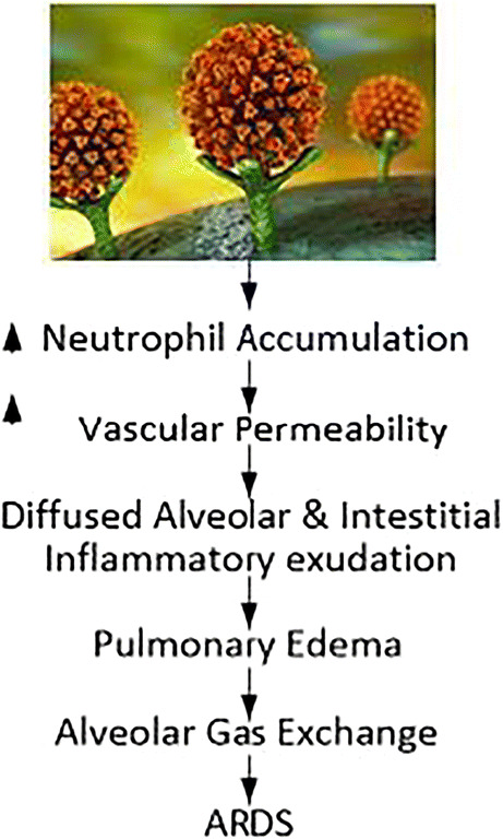
ARDS phenomenon due to SAR-CoV-2.

Comparison of COVID lung severity location with other studies

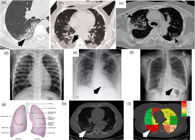
A very curial point to note here is that our system characterizes the lung region based on COVID severity. This characterization shows that all three classifiers (RF, DT, and k-NN) used in Block imaging have a more or less the same behavior in the sense that COVID severity is highest in the inferior lobe of the right lung and close to the base of the lung (near the diaphragm). This was well noted pathologically by several studies as well [2–8]. The images from existing research are shown in Fig. 25. The top row shows the COVID infected lung pointing out the COVID severity by black arrows ((a) Pan et al. [2] showing COVID severity more in the lower lung regions, (b) Wang et al. [16] similarly showing the severity of infection in lower lobes of lungs, (c) Tian et al. [5] chest CT also showing the point of infection near the lower part of the left lung). The middle row shows the chest X-ray scans of the Control and COVID patients ((d) Elasnaoui & Chawki [78] showing normal lung X-Ray, (e) Elasnaoui & Chawki [78] showing COVID lung X-Ray, (f) Aigner et al. [7] showing COVID CXR). The bottom image shows the color-coding of the probability map using Block imaging. The RED color is the highest COVID severity which matches the top row COVID severity locations (which is part of the inferior lobes, as shown in the anatomy as well).

Fig. 25.

a Pan et al. [2] showing COVID severity more in the lower lung regions, b Wang et al. [16] similarly showing the severity of infection in lower lobes of lungs, c Tian et al. [5] chest CT also shows the point of infection near the lower part of the left lung, d Elasnaoui & Chawki [78] showing normal lung X-Ray, e Elasnaoui & Chawki [78] showing COVID lung X-Ray, f Aigner et al. [7] showing COVID CXR, g image showing the anatomy of lungs, h original grayscale image from this study’s dataset with a white arrow pointing severity of infection at the bottom part of the right lung, i Block imaging showing most severity of infection in the right lower lobe of lung in RED color

Benchmarking against previous studies

Table 9 presents the benchmarking table that compares five main studies for lung tissue classification (R1 to R5). Six different attributes are used for the comparison (shown from C1 to C6). This includes the year in which it was published (column 1), the technique used (such as ML vs. DL or TL in column 2), the data size adapted in the protocol (in column 3), classification accuracy (in column 4), COVID severity (column 5) and ability to characterize the lung tissue (in column 6). Note that the unique contribution of our study comes in the way we compute the COVID severity by designing the color map superimposed on the grayscale CT lung slice. Further, we developed three different kinds of strategies for tissue characterization for COVID lungs based on (a) Block imaging strategy, (b) Bispectrum using higher-order spectra, and (c) entropy analysis. Another important accomplishment of our work is the achievement of higher accuracy even with conventional classifiers like Random Forest, which is in the range close to 100% with AUC close to 1.0 (p < 0.0001), as shown in the box (R6, C4).

Table 9.

Benchmarking of the proposed CADx study against the existing work in COVID classification and characterization

R#	C1	C2	C3	C4	C5	C6
	Author	AI-Model ML vs. DL	Data Size	Accuracy	COVID Severity	COVID Disease Characterization
R1	Zhang et al. [21] (2020)	TL-based 3-D ResNet 18	617,775 CT lung images from 4154 patients	92.49% (AUC: 0.9813)	X	X
R2	Wang et al. [22] (2020)	TL-based DenseNet-like structure	5372 patients with CT images	80.12% (AUC:0.90)	X	X
R3	Oh et al. [23] (2020)	TL-based FC-DenseNet103	13,645 patients	88.9%	X	X
R4	Yang et al. [24] (2020)	TL-based DenseNet	healthy person: 149; COVID-19 patients: 146	92% (AUC: 0.98)	X	X
R5	Wu et al. [25] (2020)	TL-based ResNet50	1018 patients (375,590 CT images)	98.23% (AUC: 0.9971)	X	X
R6	Proposed Study	ML-based classifier: RF	990 Controls and 705 COVID	99.41 ± 0.62% (AUC: 0.988) (p < 0.0001)	Block Imaging	Block Imaging, Bispectrum, Entropy
R7	Proposed Study	DL-based systems: CNN	990 Controls and 705 COVID	99.41 ± 5.12% (AUC: 0.991) (p < 0.0001)	Block Imaging	Block Imaging, Bispectrum, Entropy

TL Transfer learning, ML machine learning, RF Random Forest, DT Decision Tree, k-NN k Nearest Neighbor, AUC area under the curve.

Most of the methods which have been recently published use the transfer-learning paradigm, where the initial weights are taken from the natural images or animal data called the “ImageNet” dataset [79]. Three of the five techniques use “DenseNet” based on TL having accuracies in the low 80% or high 80% range (see row numbers: R2, R3, R4). Two of the five techniques used “ResNet-18” and “ResNet-50” (R1 and R5) having the accuracy in low 90% and one in a high 90% range. Even though we also use DL and TL, however, we do adopt a low number of features with the usage of the feature selection paradigm for ML methods.

Special note on transfer learning models

VGG16 is a pre-trained model with 13 convolution layers and 3 dense layers which gives the name VGG16 due to 13 + 3 = 16 main layers in the model. It gives the encouraging results on the ImageNet dataset and is thus use widely adapted for transfer learning in different image classification problems. The size of the weights file of VGG16 is however huge and thus to solve this problem MobileNet was introduced for deployment on mobile devices with reduced storage using width multiplier and resolution multiplier having almost a similar accuracy as VGG16. As seen from DenseNet architectures, the number of batch normalization layers gives the corresponding name of the DenseNet model. For each layer, the feature-maps of all preceding layers were used as inputs, and its own feature-maps were used as inputs into all subsequent layers. DenseNets have several advantages: they solve the vanishing-gradient problem, strengthen feature propagation, encourage feature reuse, and substantially reduce the number of parameters. The pre-trained models, however, are designed for 1000 class problems thus to design a CNN for only 2 class COVID classification problems a simpler model was needed with only 7 layers as shown in Fig. 6 and was found to give better results than pre-trained models.

Strengths

In the first part of the study, we compared one type of deep learning and 5 transfer learning-based methods of COVID classification and showed they performed with high accuracy using K10 protocol. ML classifiers were also experimented and they also showed comparable accuracy with DL models. The next part of the study demonstrated how the division of lung into blocks and carrying classification of individual blocks can help to identify the most severely affected area of the lung infected in COVID patients. This matches other research work which also tells that lower lung segments are most affected by COVID. Bispectrum after Radon transform of images also shows much higher values for COVID images, thus supporting the hypothesis of more visible areas of congestion in diseased lungs. Finally, block-wise entropy of lungs also showed more random texture in lower blocks of lungs of COVID as compared to Control patients. These three methods form a strong basis for characterizing the severity of COVID infection in affected patients. The COVID tissue characterization was validated against the ground glass opacity (GGO) values of CT scans and it was found COVID severity using block imaging showed high correlation with GGO values. Similarly, Bispectrum also showed high correlation with GGO values, thereby validating the characterization systems. Validation of classification results was also done using the Diagnostics Odds Ratio (DOR) and Receiver Operating Characteristics (ROC) curve.

Limitations

Although we used a limited size of the cohort it was demonstrated that 9 AI classification systems and 3 characterization systems gave a high performance in terms of accuracy and correlation with GGO values, ensuring that the system is reliable and foolproof. It is not unusual to see lesser cohort size in standardized journals [80, 81] and that uses AI-based technologies first time on newly acquired data sets [82–86]. Despite the novelty in CL lung characterization and classification paradigms on the Italian database, a more diversified CT lung dataset can be collected retrospectively from other parts of the world such as Asia, Europe, the Middle East, and South America for further validation of our models.

Extensions

Further, we can extend our models from ML to DL for classification and characterization of “mild COVID lung disease” vs. “other viral pneumonia lung disease”. The study can be extended for larger and diversified cohorts. We intend to bring viral pneumonia cases over time and for better multi-class ML models [87, 88]. More automated CT lung segmentation tools can be tried [11, 89, 90] as COVID data evolves and readily get available. Further, systems can undergo variability analysis in segmentation [91] and imaging different types of scanners [92]. To save time, transfer learning-based approaches can be appropriately tried in a big data framework [93]. Lastly, more sophisticated cross-modality validation can be conducted between PET and CT using registration algorithms [11, 94–96].

Conclusion

This study presented a CADx system that consisted of a two-stage system: (a) lung segmentation and (b) classification. The classification system consisted of one proposed CNN, five kinds of transfer learning methods and three different kinds of soft classifiers such as Random Forest, Decision Tree, and ANN. Further, the system also presented three kinds of lung tissue characterization systems such as Block imaging, Bispectrum analysis, and entropy analysis. Our performance evaluation criteria used diagnosis odds ratio, receiver operating characteristics, and statistical tests of the CADx system. The best performing soft classifier was proposed CNN and Random Forest having an accuracy of 99.41 ± 5.12% and AUC of 0.991 p < 0.0001 and 99.41 ± 0.62% and AUC of 0.988 p < 0.0001. The characterization system demonstrated the color-coded probability maps having the highest accuracy in the inferior lobes of the COVID lungs. Further, all three kinds of tissue characterization system gave consistent results on COVID severity locations. This is a pilot study and more aggressive data collection must be followed to further validate the system design. This pilot study was unique in its ability to perform best with limited data size and limited classes. We anticipate extending this system to multiple classes consisting of Control, mild COVID, and other viral pneumonia.

Pictorial Representation of Mean Accuracies

Mean accuracies of different ML classifiers

A plot of mean accuracies of different ML classifiers using Eq. (1) is shown in Fig. 31. A plot of mean classification over all the classifiers taken over different features using Eq. (2) is shown in Fig. 32. In Fig. 32, FC1: LBP feature, FC2: LBP and Haralick feature set, FC3: LBP, Haralick, and HOG feature set, FC4: LBP, Haralick, HOG, and Hu-moments feature set, FC5: LBP, Haralick, HOG, Hu-moments, and GLRLM feature set. The effect of the features on the ML-based classifiers is shown in Fig. 33. The figure shows the accuracy values for different feature combinations and as seen the linear regression line for all classifiers show an increase with an increase in the number of features from FC1 to FC5. Line of regression for Random Forest is highest showing the best results are obtained using RF followed by DT and then ANN. A plot of mean accuracies vs. K-fold protocols over all the classifiers and all the features using Eq. (3) is shown in Fig. 34.

Visual Representation of the risk probabilities in lung region by color codes

Fig. 39.

A sample COVID patient’s image with color coded blocks of COVID lung using k-NN classifier for a K2 b K4, c K5, and d K10 protocols

Statistical Tests for AI models

Mann Whitney, paired t-test and Kappa statistical tests were performed on the accuracy values of different classifiers. Mann Whitney tests were performed on ML classifiers for a different feature set combination as shown in Table 13.

For performing Mann Whitney tests two feature combinations were used and 3 K10 mean accuracy values of ANN, DT and RF were fed to obtain a z score, p value and Mann Whitney U value as shown in Table 14.

The Mann Whitney U value indicates the number of times first feature set values are more than the second feature set. The maximum U value is n1*n2 where n1 and n2 are the sample size of 2 feature set, here n1 = n2 = 3. Thus, the maximum possible U in our case is 9 and the minimum possible value of U is 0. The probability is more than 0.05 in all cases thus we can use all feature set interchangeably. This means they are giving similar results. A sample screen

shot of Mann Whitney test between FC1 and FC2 using MedCalc software is shown in Fig. 42.

Paired t-tests were performed between 10 combinations of K10 protocol for TL classifiers versus ML, DL versus ML classifiers and DL versus TL classifiers as shown in Tables 15, 16 and 17 respectively. A sample screenshot of paired t-test between CNN and RF using MedCalc software is shown in Fig. 43.

Fig. 43.

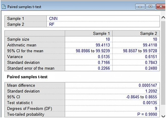
A sample screen shot of paired t-test for 10 combinations of K10 protocol for CNN and RF

The negative t values in paired t-tests indicate that the second classifier mean is less than the first classifier mean. The p values less than 0.05 means that there is a significant difference between the 2 classifiers accuracies. The p values more than 0.05 means that 2 classifiers can be used interchangeably. Thus, based on this classifier which can be used interchangeably are:

• DenseNet121-ANN

• MobileNet-ANN

• DenseNet201-ANN

• DenseNet169-ANN

• CNN-RF

Classifiers which differ significantly are:

• DenseNet121-DT

• DenseNet121-RF

• MobileNet-DT

• MobileNet-RF

• DenseNet201-DT

• DenseNet201-RF

• DenseNet169-DT

• DenseNet169-RF

• VGG16-ANN

• VGG16-DT

• VGG16-RF

• CNN-ANN

• CNN-DT

• CNN-DenseNet121

• CNN-MobileNet

• CNN-DenseNet201

• CNN-DenseNet169

• CNN-VGG16

In addition to Mann Whitney and paired t-tests, Cohen Kappa tests were also performed on all classifiers and its results are shown as Column C9 of Table 8. It is clearly seen Kappa score increases with increasing accuracy and is maximum for CNN and RF.

Fig. 42.

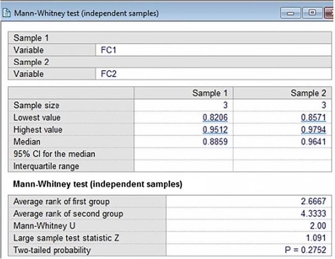
A sample screen shot of Mann Whitney test on FC1 and FC2 for ANN, DT and RF K10 accuracies

Symbol Table

Table 18.

Symbol Table

SN	Symbol	Description of Symbol
1	pi	Probability of pixel intensity
2	B	Bispectrum value
3	μControl	Mean feature strength for control class
4	μCOVID	Mean feature strength of COVID class
5	Se	Sensitivity
6	Sp	Specificity
7	F	Fourier transform
8	E	Expectation operator
9	DL	Deep Learning
10	TL	Transfer learning
11	k -NN	k-Nearest neighbor
12	ANN	Artificial Neural Network
13	DT	Decision tree
14	RF	Random Forest
15	K2	2-fold cross-validation
16	K4	4-fold cross-validation
17	K5	5-fold cross-validation
18	K10	10-fold cross-validation

Compliance with ethical standards

Conflict of interest

All authors declare that they have no conflict of interest.

Ethical approval

All procedures performed in studies involving human participants were in accordance with the ethical standards of the institutional and/or national research committee and with the 1964 Helsinki declaration and its later amendments or comparable ethical standards.

Informed consent

Informed consent was obtained from all individual participants included in the study.

References

- 1.Yuen K-S, Ye Z-W, Fung S-Y, Chan C-P, Jin D-Y. Sars-cov-2 and covid-19: The most important research questions. Cell Biosci. 2020;10(1):1–5. doi: 10.1186/s13578-020-00404-4. [DOI] [PMC free article] [PubMed] [Google Scholar]
- 2.F. Pan, T. Ye, P. Sun, S. Gui, B. Liang, L. Li, D. Zheng, J. Wang, R. L. Hesketh, L. Yang, et al., Time course of lung changes on chest ct during recovery from 2019 novel coronavirus (covid-19) pneumonia, Radiology (2020) 200370. [DOI] [PMC free article] [PubMed]
- 3.H. Y. F. Wong, H. Y. S. Lam, A. H.-T. Fong, S. T. Leung, T. W.-Y. Chin, C. S. Y. Lo, M. M.-S. Lui, J. C. Y. Lee, K. W.-H. Chiu, T. Chung, et al., Frequency and distribution of chest radiographic findings in covid-19 positive patients, Radiology (2020) 201160. [DOI] [PMC free article] [PubMed]
- 4.M. Smith, S. Hayward, S. Innes, A. Miller, Point-of-care lung ultrasound in patients with covid-19–a narrative review, Anaesthesia (2020). [DOI] [PMC free article] [PubMed]
- 5.S. Tian, W. Hu, L. Niu, H. Liu, H. Xu, S.-Y. Xiao, Pulmonary pathology of early phase 2019 novel coronavirus (covid-19) pneumonia in two patients with lung cancer, J Thorac Oncol (2020). [DOI] [PMC free article] [PubMed]
- 6.Ackermann M, Verleden SE, Kuehnel M, Haverich A, Welte T, Laenger F, Vanstapel A, Werlein C, Stark H, Tzankov A, et al. Pulmonary vascular endothelialitis, thrombosis, and angiogenesis in covid-19, New England Journal of Medicine. 2020. [DOI] [PMC free article] [PubMed] [Google Scholar]
- 7.Aigner C, Dittmer U, Kamler M, Collaud S, Taube C. Covid-19 in a lung transplant recipient. J Heart Lung Transplant. 2020;39(6):610. doi: 10.1016/j.healun.2020.04.004. [DOI] [PMC free article] [PubMed] [Google Scholar]
- 8.Q.-Y. Peng, X.-T. Wang, L.-N. Zhang, C. C. C. U. S. Group, et al., Findings of lung ultrasonography of novel corona virus pneumonia during the 2019–2020 epidemic, Intensive Care Med (2020) 1. [DOI] [PMC free article] [PubMed]
- 9.Saba L, Gerosa C, Fanni D, Marongiu F, La Nasa G, Caocci G, Barcellona D, Balestrieri A, Coghe F, Orru G, et al. Molecular pathways triggered by covid-19 in different organs: Ace2 receptorexpressing cells under attack? a review. Eur Rev Med Pharmacol Sci. 2020;24:12609–12622. doi: 10.26355/eurrev_202012_24058. [DOI] [PubMed] [Google Scholar]
- 10.R. Cau, P. P. Bassareo, L. Mannelli, J. S. Suri, L. Saba, Imaging in covid-19-related myocardial injury, Int J Cardiovasc Imaging (2020) 1–12. [DOI] [PMC free article] [PubMed]
- 11.A. El-Baz, J. S. Suri, Lung imaging and computer aided diagnosis, CRC Press, 2011.
- 12.R. M. Rangayyan, J. S. Suri, Recent Advances in Breast Imaging, Mammography, and ComputerAided Diagnosis of Breast Cancer., SPIE Publications, 2006.
- 13.Narayanan R, Werahera P, Barqawi A, Crawford E, Shinohara K, Simoneau A, Suri J. Adaptation of a 3d prostate cancer atlas for transrectal ultrasound guided target-specific biopsy. Phys Med Biol. 2008;53(20):N397. doi: 10.1088/0031-9155/53/20/N03. [DOI] [PubMed] [Google Scholar]
- 14.J. S. Suri, A. Puvvula, M. Biswas, M. Majhail, L. Saba, G. Faa, I. M. Singh, R. Oberleitner, M. Turk, P. S. Chadha, et al., Covid-19 pathways for brain and heart injury in comorbidity patients: A role of medical imaging and artificial intelligence-based covid severity classification: A review, Comput Biol Med (2020) 103960. [DOI] [PMC free article] [PubMed]
- 15.O. Gozes, M. Frid-Adar, H. Greenspan, P. D. Browning, H. Zhang, W. Ji, A. Bernheim, E. Siegel, Rapid ai development cycle for the coronavirus (covid-19) pandemic: Initial results for automated detection & patient monitoring using deep learning ct image analysis, arXiv preprint arXiv:2003.05037 (2020).
- 16.S. Wang, B. Kang, J. Ma, X. Zeng, M. Xiao, J. Guo, M. Cai, J. Yang, Y. Li, X. Meng, et al., A deep learning algorithm using ct images to screen for corona virus disease (covid-19), MedRxiv (2020). [DOI] [PMC free article] [PubMed]
- 17.I. D. Apostolopoulos, T. A. Mpesiana, Covid-19: automatic detection from x-ray images utilizing transfer learning with convolutional neural networks, Phys Eng Sci Med (2020) 1. [DOI] [PMC free article] [PubMed]
- 18.C. Butt, J. Gill, D. Chun, B. A. Babu, Deep learning system to screen coronavirus disease 2019 pneumonia, Appl Intell (2020) 1. [DOI] [PMC free article] [PubMed]
- 19.L. Wang, A. Wong, Covid-net: A tailored deep convolutional neural network design for detection of covid-19 cases from chest x-ray images, arXiv preprint arXiv:2003.09871 (2020). [DOI] [PMC free article] [PubMed]
- 20.A. Narin, C. Kaya, Z. Pamuk, Automatic detection of coronavirus disease (covid-19) using x-ray images and deep convolutional neural networks, arXiv preprint arXiv:2003.10849 (2020). [DOI] [PMC free article] [PubMed]
- 21.Zhang K, Liu X, Shen J, Li Z, Sang Y, Wu X, Zha Y, Liang W, Wang C, Wang K, et al. Clinically applicable ai system for accurate diagnosis, quantitative measurements, and prognosis of covid-19 pneumonia using computed tomography, Cell. 2020. [DOI] [PMC free article] [PubMed] [Google Scholar]
- 22.S. Wang, Y. Zha, W. Li, Q. Wu, X. Li, M. Niu, M. Wang, X. Qiu, H. Li, H. Yu, et al., A fully automatic deep learning system for covid-19 diagnostic and prognostic analysis, Eur Respir J (2020). [DOI] [PMC free article] [PubMed]
- 23.Y. Oh, S. Park, J. C. Ye, Deep learning covid-19 features on cxr using limited training data sets, IEEE Trans Med Imaging (2020). [DOI] [PubMed]
- 24.S. Yang, L. Jiang, Z. Cao, L. Wang, J. Cao, R. Feng, Z. Zhang, X. Xue, Y. Shi, F. Shan, Deep learning for detecting corona virus disease 2019 (covid-19) on high-resolution computed tomography: a pilot study, Annals of Translational Medicine 8 (7) (2020). [DOI] [PMC free article] [PubMed]
- 25.Wu P, Sun X, Zhao Z, Wang H, Pan S, Schuller B. Classification of lung nodules based on deep residual networks and migration learning, Computational Intelligence and Neuroscience 2020. 2020. [DOI] [PMC free article] [PubMed] [Google Scholar]
- 26.Skandha SS, Gupta SK, Saba L, Koppula VK, Johri AM, Khanna NN, Mavrogeni S, Laird JR, Pareek G, Miner M, et al. 3-d optimized classification and characterization artificial intelligence paradigm for cardiovascular/stroke risk stratification using carotid ultrasound-based delineated plaque: Atheromatic 2.0. Comput Biol Med. 2020;125:103958. doi: 10.1016/j.compbiomed.2020.103958. [DOI] [PubMed] [Google Scholar]
- 27.Wang S, Summers RM. Machine learning and radiology. Med Image Anal. 2012;16(5):933–951. doi: 10.1016/j.media.2012.02.005. [DOI] [PMC free article] [PubMed] [Google Scholar]
- 28.Wernick MN, Yang Y, Brankov JG, Yourganov G, Strother SC. Machine learning in medical imaging. IEEE Signal Process Mag. 2010;27(4):25–38. doi: 10.1109/MSP.2010.936730. [DOI] [PMC free article] [PubMed] [Google Scholar]
- 29.Prasadl B, Prasad P, Sagar Y. An approach to develop expert systems in medical diagnosis using machine learning algorithms (asthma) and a performance study. Int J on Soft Comput (IJSC) 2011;2(1):26–33. doi: 10.5121/ijsc.2011.2103. [DOI] [Google Scholar]
- 30.Erickson BJ, Korfiatis P, Akkus Z, Kline TL. Machine learning for medical imaging. Radiographics. 2017;37(2):505–515. doi: 10.1148/rg.2017160130. [DOI] [PMC free article] [PubMed] [Google Scholar]
- 31.Maniruzzaman M, Kumar N, Abedin MM, Islam MS, Suri HS, El-Baz AS, Suri JS. Comparative approaches for classification of diabetes mellitus data: Machine learning paradigm. Comput Methods Prog Biomed. 2017;152:23–34. doi: 10.1016/j.cmpb.2017.09.004. [DOI] [PubMed] [Google Scholar]
- 32.Maniruzzaman M, Rahman MJ, Al-MehediHasan M, Suri HS, Abedin MM, El-Baz A, Suri JS. Accurate diabetes risk stratification using machine learning: role of missing value and outliers. J Med Syst. 2018;42(5):92. doi: 10.1007/s10916-018-0940-7. [DOI] [PMC free article] [PubMed] [Google Scholar]
- 33.Maniruzzaman M, Rahman MJ, Ahammed B, Abedin MM, Suri HS, Biswas M, El-Baz A, Bangeas P, Tsoulfas G, Suri JS. Statistical characterization and classification of colon microarray gene expression data using multiple machine learning paradigms. Comput Methods Prog Biomed. 2019;176:173–193. doi: 10.1016/j.cmpb.2019.04.008. [DOI] [PubMed] [Google Scholar]
- 34.Nikias CL, Hsing-Hsing C. Higher-order spectrum estimation via noncausal autoregressive modeling and deconvolution. IEEE Trans Acoust Speech Signal Process. 1988;36(12):1911–1913. doi: 10.1109/29.9037. [DOI] [Google Scholar]
- 35.Glas AS, Lijmer JG, Prins MH, Bonsel GJ, Bossuyt PM. The diagnostic odds ratio: a single indicator of test performance. J Clin Epidemiol. 2003;56(11):1129–1135. doi: 10.1016/S0895-4356(03)00177-X. [DOI] [PubMed] [Google Scholar]
- 36.Noor NM, Than JC, Rijal OM, Kassim RM, Yunus A, Zeki AA, Anzidei M, Saba L, Suri JS. Automatic lung segmentation using control feedback system: morphology and texture paradigm. J Med Syst. 2015;39(3):22. doi: 10.1007/s10916-015-0214-6. [DOI] [PubMed] [Google Scholar]
- 37.Than JC, Saba L, Noor NM, Rijal OM, Kassim RM, Yunus A, Suri HS, Porcu M, Suri JS. Lung disease stratification using amalgamation of riesz and gabor transforms in machine learning framework. Comput Biol Med. 2017;89:197–211. doi: 10.1016/j.compbiomed.2017.08.014. [DOI] [PubMed] [Google Scholar]
- 38.Nolf EX, Voet T, Jacobs F, Dierckx R, Lemahieu I. An open-source medical image conversion toolkit. Eur J Nucl Med. 2003;30(Suppl 2):S246. [Google Scholar]
- 39.Saba L, Dey N, Ashour AS, Samanta S, Nath SS, Chakraborty S, Sanches J, Kumar D, Marinho R, Suri JS. Automated stratification of liver disease in ultrasound: an online accurate feature classification paradigm. Comput Methods Prog Biomed. 2016;130:118–134. doi: 10.1016/j.cmpb.2016.03.016. [DOI] [PubMed] [Google Scholar]
- 40.Acharya UR, Sree SV, Ribeiro R, Krishnamurthi G, Marinho RT, Sanches J, Suri JS. Data mining framework for fatty liver disease classification in ultrasound: a hybrid feature extraction paradigm. Med Phys. 2012;39(7Part1):4255–4264. doi: 10.1118/1.4725759. [DOI] [PubMed] [Google Scholar]
- 41.Kuppili V, Biswas M, Sreekumar A, Suri HS, Saba L, Edla DR, Marinho RT, Sanches JM, Suri JS. Author correction to: Extreme learning machine framework for risk stratification of fatty liver disease using ultrasound tissue characterization. J Med Syst. 2017;42(1):18. doi: 10.1007/s10916-017-0862-9. [DOI] [PubMed] [Google Scholar]
- 42.Molinari F, Mantovani A, Deandrea M, Limone P, Garberoglio R, Suri JS. Characterization of single thyroid nodules by contrast-enhanced 3-d ultrasound. Ultrasound Med Biol. 2010;36(10):1616–1625. doi: 10.1016/j.ultrasmedbio.2010.07.011. [DOI] [PubMed] [Google Scholar]
- 43.Acharya UR, Swapna G, Sree SV, Molinari F, Gupta S, Bardales RH, Witkowska A, Suri JS. A review on ultrasound-based thyroid cancer tissue characterization and automated classification. Technology in cancer research & treatment. 2014;13(4):289–301. doi: 10.7785/tcrt.2012.500381. [DOI] [PubMed] [Google Scholar]
- 44.Acharya U, Vinitha Sree S, Mookiah M, Yantri R, Molinari F, Ziele’znik W, Ma lyszekTumidajewicz J, Stepie’n B, Bardales R, Witkowska A, et al. Diagnosis of hashimoto’s thyroiditis in ultrasound using tissue characterization and pixel classification, Proceedings of the Institution of Mechanical Engineers. Part H: J Eng Med. 2013;227(7):788–798. doi: 10.1177/0954411913483637. [DOI] [PubMed] [Google Scholar]
- 45.Acharya UR, Molinari F, Sree SV, Swapna G, Saba L, Guerriero S, Suri JS. Ovarian tissue characterization in ultrasound: a review. Technol Cancer Res Treat. 2015;14(3):251–261. doi: 10.1177/1533034614547445. [DOI] [PubMed] [Google Scholar]
- 46.Acharya UR, Sree SV, Kulshreshtha S, Molinari F, Koh JEW, Saba L, Suri JS. Gynescan: an improved online paradigm for screening of ovarian cancer via tissue characterization. Technol Cancer Res Treat. 2014;13(6):529–539. doi: 10.7785/tcrtexpress.2013.600273. [DOI] [PMC free article] [PubMed] [Google Scholar]
- 47.Acharya UR, Mookiah MRK, Sree SV, Yanti R, Martis R, Saba L, Molinari F, Guerriero S, Suri JS. Evolutionary algorithm-based classifier parameter tuning for automatic ovarian cancer tissue characterization and classification. Ultraschall in der Medizin-Eur J Ultrasound. 2014;35(03):237–245. doi: 10.1055/s-0032-1330336. [DOI] [PubMed] [Google Scholar]
- 48.Acharya UR, Mookiah MRK, Sree SV, Afonso D, Sanches J, Shafique S, Nicolaides A, Pedro LM, Fernandes JF e, Suri JS. Atherosclerotic plaque tissue characterization in 2d ultrasound longitudinal carotid scans for automated classification: a paradigm for stroke risk assessment. Med Biol Eng Comput. 2013;51(5):513–523. doi: 10.1007/s11517-012-1019-0. [DOI] [PubMed] [Google Scholar]
- 49.J. S. Suri, C. Kathuria, F. Molinari, Atherosclerosis disease management, Springer Science & Business Media, 2010.
- 50.Acharya UR, Faust O, Sree SV, Molinari F, Saba L, Nicolaides A, Suri JS. An accurate and generalized approach to plaque characterization in 346 carotid ultrasound scans. IEEE Trans Instrum Meas. 2011;61(4):1045–1053. doi: 10.1109/TIM.2011.2174897. [DOI] [Google Scholar]
- 51.Saba L, Jain PK, Suri HS, Ikeda N, Araki T, Singh BK, Nicolaides A, Shafique S, Gupta A, Laird JR, et al. Plaque tissue morphology-based stroke risk stratification using carotid ultrasound: a polling-based pca learning paradigm. J Med Syst. 2017;41(6):98. doi: 10.1007/s10916-017-0745-0. [DOI] [PubMed] [Google Scholar]
- 52.Acharya UR, Faust O, Alvin A, Krishnamurthi G, Seabra JC, Sanches J, Suri JS, et al. Understanding symptomatology of atherosclerotic plaque by image-based tissue characterization. Comput Methods Prog Biomed. 2013;110(1):66–75. doi: 10.1016/j.cmpb.2012.09.008. [DOI] [PubMed] [Google Scholar]
- 53.Acharya UR, Faust O, Sree SV, Alvin APC, Krishnamurthi G, Sanches J, Suri JS, et al. 2011 Annual International Conference of the IEEE Engineering in Medicine and Biology Society, IEEE. 2011. Atheromatic: Symptomatic vs. asymptomatic classification of carotid ultrasound plaque using a combination of hos, dwt & texture; pp. 4489–4492. [DOI] [PubMed] [Google Scholar]
- 54.Acharya U, Sree SV, Mookiah M, Saba L, Gao H, Mallarini G, Suri J. Computed tomography carotid wall plaque characterization using a combination of discrete wavelet transform and texture features: A pilot study. Proc Inst Mech Eng H J Eng Med. 2013;227(6):643–654. doi: 10.1177/0954411913480622. [DOI] [PubMed] [Google Scholar]
- 55.Acharya UR, Sree SV, Krishnan MMR, Saba L, Molinari F, Guerriero S, Suri JS. Ovarian tumor characterization using 3d ultrasound. Technol Cancer Res Treat. 2012;11(6):543–552. doi: 10.7785/tcrt.2012.500272. [DOI] [PubMed] [Google Scholar]
- 56.Martis RJ, Acharya UR, Prasad H, Chua CK, Lim CM, Suri JS. Application of higher order statistics for atrial arrhythmia classification. Biomed Signal Process Control. 2013;8(6):888–900. doi: 10.1016/j.bspc.2013.08.008. [DOI] [Google Scholar]
- 57.Pareek G, Acharya UR, Sree SV, Swapna G, Yantri R, Martis RJ, Saba L, Krishnamurthi G, Mallarini G, El-Baz A, et al. Prostate tissue characterization/classification in 144 patient population using wavelet and higher order spectra features from transrectal ultrasound images. Technol Cancer Res Treat. 2013;12(6):545–557. doi: 10.7785/tcrt.2012.500346. [DOI] [PubMed] [Google Scholar]
- 58.Acharya UR, Sree SV, Krishnan MMR, Krishnananda N, Ranjan S, Umesh P, Suri JS. Automated classification of patients with coronary artery disease using grayscale features from left ventricle echocardiographic images. Comput Methods Prog Biomed. 2013;112(3):624–632. doi: 10.1016/j.cmpb.2013.07.012. [DOI] [PubMed] [Google Scholar]
- 59.Shrivastava VK, Londhe ND, Sonawane RS, Suri JS. Computer-aided diagnosis of psoriasis skin images with hos, texture and color features: a first comparative study of its kind. Comput Methods Prog Biomed. 2016;126:98–109. doi: 10.1016/j.cmpb.2015.11.013. [DOI] [PubMed] [Google Scholar]
- 60.Acharya UR, Faust O, Sree V, Swapna G, Martis RJ, Kadri NA, Suri JS. Linear and nonlinear analysis of normal and cad-affected heart rate signals. Comput Methods Prog Biomed. 2014;113(1):55–68. doi: 10.1016/j.cmpb.2013.08.017. [DOI] [PubMed] [Google Scholar]
- 61.Acharya UR, Sree SV, Molinari F, Saba L, Nicolaides A, Suri JS. An automated technique for carotid far wall classification using grayscale features and wall thickness variability. J Clin Ultrasound. 2015;43(5):302–311. doi: 10.1002/jcu.22183. [DOI] [PubMed] [Google Scholar]
- 62.Acharya RU, Faust O, Alvin APC, Sree SV, Molinari F, Saba L, Nicolaides A, Suri JS. Symptomatic vs. asymptomatic plaque classification in carotid ultrasound. J Med Syst. 2012;36(3):1861–1871. doi: 10.1007/s10916-010-9645-2. [DOI] [PubMed] [Google Scholar]
- 63.Jamthikar A, Gupta D, Saba L, Khanna NN, Araki T, Viskovic K, Mavrogeni S, Laird JR, Pareek G, Miner M, et al. Cardiovascular/stroke risk predictive calculators: a comparison between statistical and machine learning models. Cardiovasc Diagn Ther. 2020;10(4):919. doi: 10.21037/cdt.2020.01.07. [DOI] [PMC free article] [PubMed] [Google Scholar]
- 64.Jamthikar A, Gupta D, Khanna NN, Saba L, Laird JR, Suri JS. Cardiovascular/stroke risk prevention: a new machine learning framework integrating carotid ultrasound image-based phenotypes and its harmonics with conventional risk factors. Indian Heart J. 2020;72(4):258–264. doi: 10.1016/j.ihj.2020.06.004. [DOI] [PMC free article] [PubMed] [Google Scholar]
- 65.Viswanathan V, Jamthikar AD, Gupta D, Shanu N, Puvvula A, Khanna NN, Saba L, Omerzum T, Viskovic K, Mavrogeni S, et al. Low-cost preventive screening using carotid ultrasound in patients with diabetes. Frontiers in Bioscience (Landmark Edition) 2020;25:1132–1171. doi: 10.2741/4850. [DOI] [PubMed] [Google Scholar]
- 66.Kadam P, Bhalerao S. Sample size calculation. Int J Ayurveda Res. 2010;1(1):55. doi: 10.4103/0974-7788.59946. [DOI] [PMC free article] [PubMed] [Google Scholar]
- 67.M. Hoffmann, H. Kleine-Weber, S. Schroeder, N. Krüger, T. Herrler, S. Erichsen, T. S. Schiergens, G. Herrler, N.-H. Wu, A. Nitsche, et al., Sars-cov-2 cell entry depends on ace2 and tmprss2 and is blocked by a clinically proven protease inhibitor, Cell (2020). [DOI] [PMC free article] [PubMed]
- 68.De Wit E, Van Doremalen N, Falzarano D, Munster VJ. Sars and mers: recent insights into emerging coronaviruses. Nat Rev Microbiol. 2016;14(8):523. doi: 10.1038/nrmicro.2016.81. [DOI] [PMC free article] [PubMed] [Google Scholar]
- 69.Wu K, Peng G, Wilken M, Geraghty RJ, Li F. Mechanisms of host receptor adaptation by severe acute respiratory syndrome coronavirus. J Biol Chem. 2012;287(12):8904–8911. doi: 10.1074/jbc.M111.325803. [DOI] [PMC free article] [PubMed] [Google Scholar]
- 70.Patel VB, Zhong J-C, Grant MB, Oudit GY. Role of the ace2/angiotensin 1–7 axis of the renin–angiotensin system in heart failure. Circ Res. 2016;118(8):1313–1326. doi: 10.1161/CIRCRESAHA.116.307708. [DOI] [PMC free article] [PubMed] [Google Scholar]
- 71.X. Zou, K. Chen, J. Zou, P. Han, J. Hao, Z. Han, Single-cell rna-seq data analysis on the receptor ace2 expression reveals the potential risk of different human organs vulnerable to 2019-ncov infection, Front Med (2020) 1–8. [DOI] [PMC free article] [PubMed]
- 72.Hamming I, Timens W, Bulthuis M, Lely A, Navis GV, van Goor H. Tissue distribution of ace2 protein, the functional receptor for sars coronavirus. a first step in understanding sars pathogenesis. J Pathol: J Pathol Soc Great Britain Ireland. 2004;203(2):631–637. doi: 10.1002/path.1570. [DOI] [PMC free article] [PubMed] [Google Scholar]
- 73.Zhang H, Baker A. Recombinant human ace2: acing out angiotensin ii in ards therapy. 2017. [DOI] [PMC free article] [PubMed] [Google Scholar]
- 74.P. Radermacher, S. M. Maggiore, A. Mercat, Fifty years of research in ards. gas exchange in acute respiratory distress syndrome, Am J Respir Crit Care Med 196 (8) 964–984. [DOI] [PubMed]
- 75.Chen N, Zhou M, Dong X, Qu J, Gong F, Han Y, Qiu Y, Wang J, Liu Y, Wei Y, et al. Epidemiological and clinical characteristics of 99 cases of 2019 novel coronavirus pneumonia in wuhan, china: a descriptive study. Lancet. 2020;395(10223):507–513. doi: 10.1016/S0140-6736(20)30211-7. [DOI] [PMC free article] [PubMed] [Google Scholar]
- 76.T.-Y. Xiong, S. Redwood, B. Prendergast, M. Chen, Coronaviruses and the cardiovascular system: acute and long-term implications, Eur Heart J (2020). [DOI] [PMC free article] [PubMed]
- 77.Oudit G, Kassiri Z, Jiang C, Liu P, Poutanen S, Penninger J, Butany J. Sars-coronavirus modulation of myocardial ace2 expression and inflammation in patients with sars. Eur J Clin Investig. 2009;39(7):618–625. doi: 10.1111/j.1365-2362.2009.02153.x. [DOI] [PMC free article] [PubMed] [Google Scholar]
- 78.K. Elasnaoui, Y. Chawki, Using x-ray images and deep learning for automated detection of coronavirus disease, J Biomol Struct Dynamics (just-accepted) (2020) 1–22. [DOI] [PMC free article] [PubMed]
- 79.J. Deng, W. Dong, R. Socher, L.-J. Li, K. Li, L. Fei-Fei, Imagenet: A large-scale hierarchical image database, in: 2009 IEEE conference on computer vision and pattern recognition, IEEE, 2009, pp. 248–255.
- 80.Porcu M, Garofalo P, Craboledda D, Suri JS, Suri HS, Montisci R, Sanfilippo R, Saba L. Carotid artery stenosis and brain connectivity: the role of white matter hyperintensities. Neuroradiology. 2020;62(3):377–387. doi: 10.1007/s00234-019-02327-5. [DOI] [PubMed] [Google Scholar]
- 81.Saba L, Argioas GM, Lucatelli P, Lavra F, Suri JS, Wintermark M. Variation of degree of stenosis quantification using different energy level with dual energy ct scanner. Neuroradiology. 2019;61(3):285–291. doi: 10.1007/s00234-018-2142-x. [DOI] [PubMed] [Google Scholar]
- 82.Araki T, Ikeda N, Shukla D, Londhe ND, Shrivastava VK, Banchhor SK, Saba L, Nicolaides A, Shafique S, Laird JR, et al. A new method for ivus-based coronary artery disease risk stratification: a link between coronary & carotid ultrasound plaque burdens. Comput Methods Prog Biomed. 2016;124:161–179. doi: 10.1016/j.cmpb.2015.10.022. [DOI] [PubMed] [Google Scholar]
- 83.Banchhor SK, Londhe ND, Araki T, Saba L, Radeva P, Laird JR, Suri JS. Wall-based measurement features provides an improved ivus coronary artery risk assessment when fused with plaque texture-based features during machine learning paradigm. Comput Biol Med. 2017;91:198–212. doi: 10.1016/j.compbiomed.2017.10.019. [DOI] [PubMed] [Google Scholar]
- 84.Banchhor SK, Londhe ND, Saba L, Radeva P, Laird JR, Suri JS. Relationship between automated coronary calcium volumes and a set of manual coronary lumen volume, vessel volume and atheroma volume in japanese diabetic cohort. J Clin Diagn Res. 2017;11(6):TC09. doi: 10.7860/JCDR/2017/26336.10030. [DOI] [PMC free article] [PubMed] [Google Scholar]
- 85.Araki T, Ikeda N, Shukla D, Jain PK, Londhe ND, Shrivastava VK, Banchhor SK, Saba L, Nicolaides A, Shafique S, et al. Pca-based polling strategy in machine learning framework for coronary artery disease risk assessment in intravascular ultrasound: a link between carotid and coronary grayscale plaque morphology. Comput Methods Prog Biomed. 2016;128:137–158. doi: 10.1016/j.cmpb.2016.02.004. [DOI] [PubMed] [Google Scholar]
- 86.Araki T, Banchhor SK, Londhe ND, Ikeda N, Radeva P, Shukla D, Saba L, Balestrieri A, Nicolaides A, Shafique S, et al. Reliable and accurate calcium volume measurement in coronary artery using intravascular ultrasound videos. J Med Syst. 2016;40(3):51. doi: 10.1007/s10916-015-0407-z. [DOI] [PubMed] [Google Scholar]
- 87.G. S. Tandel, A. Balestrieri, T. Jujaray, N. N. Khanna, L. Saba, J. S. Suri, Multiclass magnetic resonance imaging brain tumor classification using artificial intelligence paradigm, Comput Biol Med (2020) 103804. [DOI] [PubMed]
- 88.A. D. Jamthikar, D. Gupta, L. E. Mantella, L. Saba, J. R. Laird, A. M. Johri, J. S. Suri, Multiclass machine learning vs. conventional calculators for stroke/cvd risk assessment using carotid plaque predictors with coronary angiography scores as gold standard: a 500 participants study, Int J Cardiovasc Imaging (2020) 1–17. [DOI] [PubMed]
- 89.A. El-Baz, X. Jiang, J. S. Suri, Biomedical image segmentation: advances and trends, CRC Press, 2016.
- 90.A. El-Baz, G. Gimel’farb, J. S. Suri, Stochastic modeling for medical image analysis, CRC Press, 2015.
- 91.Saba L, Than JC, Noor NM, Rijal OM, Kassim RM, Yunus A, Ng CR, Suri JS. Interobserver variability analysis of automatic lung delineation in normal and disease patients. J Med Syst. 2016;40(6):142. doi: 10.1007/s10916-016-0504-7. [DOI] [PubMed] [Google Scholar]
- 92.Molinari F, Liboni W, Giustetto P, Badalamenti S, Suri JS. Automatic computer-based tracings (act) in longitudinal 2-d ultrasound images using different scanners. J Mech Med Biol. 2009;9(04):481–505. doi: 10.1142/S0219519409003115. [DOI] [Google Scholar]
- 93.A. El-Baz, J. S. Suri, Big Data in Multimodal Medical Imaging, CRC Press, 2019.
- 94.R. Narayanan, J. Kurhanewicz, K. Shinohara, E. D. Crawford, A. Simoneau, J. S. Suri, Mri-ultrasound registration for targeted prostate biopsy, in: 2009 IEEE International Symposium on Biomedical Imaging: From Nano to Macro, IEEE, 2009, pp. 991–994.
- 95.Acharya R, Ng YE, Suri JS. Image modeling of the human eye. 2008. [Google Scholar]
- 96.Liu K, Suri JS. Automatic vessel indentification for angiographic screening. uS Patent. 2005;6:845. [Google Scholar]