A SIR-type model describing the successive waves of COVID-19

Abstract

It is well-known that the classical SIR model is unable to make accurate predictions on the course of illnesses such as COVID-19. In this paper, we show that the official data released by the authorities of several countries (Italy, Spain and The USA) regarding the expansion of COVID-19 are compatible with a non-autonomous SIR type model with vital dynamics and non-constant population, calibrated according to exponentially decaying infection and death rates. Using this calibration we construct a model whose outcomes for most relevant epidemiological paramenters, such as the number of active cases, cumulative deaths, daily new deaths and daily new cases (among others) fit available real data about the first and successive waves of COVID-19. In addition to this, we also provide predictions on the evolution of this pandemic in Italy and the USA in several plausible scenarios.

1. Introduction

The problem of infectious diseases and their control has been the focus of attention in the scientific world throughout history and, more specifically, in the last decades. The problem with illnesses such as Gonorrhea Transmission [1] or the $HIV$ epidemics driven by late disease-stage transmission [2] were the focus of attention for mathematicians and physicists looking for some sort of mathematical modeling in order to predict the evolution of these undesirable infectious illnesses (see, also, [3]). More recently, researchers were also interested in the mathematical modeling of the spreading of the virus called Ebola [4]. Research works working on strategies on how to mitigate an influenza pandemic were carried out in the last decades [5]. Some references devoted completely or in part to mathematical epidemiology are [6], [7], [8], [9], [10], [11], [12], [13].

The so-called SIR models are among the simplest compartmental models. The birth of these compartmental models dates back to 1927, with the seminal work of Kermack and McKendrick [14]. The simplest SIR model is the one without the so-called vital dynamics (which includes birth and death and some demographical data) and is described by means of 3 ordinary differential equations whose variables are S, the susceptible population, I, the infected population, and R, the recovered population:

$$\{\begin{array}{ccc}\hfill S^{\prime }& =& -\beta SI,\hfill \\ \hfill I^{\prime }& =& \beta SI-\gamma I,\hfill \\ \hfill R^{\prime }& =& \gamma I,\hfill \end{array}$$ (1.1)

where $\beta$ is the transmission rate, and $\gamma$ the recuperation rate. Although this model is nonlinear, it can be analytically solved [15].

Observe that in the classical SIR model (1.2) the total population $N=S+I+R$ is assumed to be constant since $N^{\prime }=S^{\prime }+I^{\prime }+R^{\prime }=0$. This is just one of a number of facts that make model (1.2) unrealistic. In addition, it does not consider neither births nor deaths, not even those produced by the infection under study. Also, the fact that $\beta$ and $\gamma$ are constant, does not reflect the impact of realistic measures such as social distancing or scientific breakthroughs. Fig. 1 shows how far the classical SIR model is from modeling correctly the course of COVID-19 in a specific territory.

Fig. 1.

In these graphs we have depicted in red the evolution of active cases of COVID-19 in Italy between the 20th of march 2020 (zero in the horizontal axis) and the 29th of April 2020 (tick 39 in the horizontal axis). In blue we have depicted the evolution predicted by the classical SIR model calibrated with the data released by the Italian authorities on the 20th of march 2020. It can be clearly seen that the classical SIR model is not an adequate tool to model this pandemic. (For interpretation of the references to color in this figure legend, the reader is referred to the web version of this article.)

What we propose below is a mathematical model that preserves, to some extent, the simplicity of the classical SIR model, but at the same time predicts with a considerable accuracy the evolution of COVID-19 under certain reasonable assumptions. The model is tested with the official data regarding the course of COVID-19 in Italy, Spain and The US.

The COVID-19 pandemic, also known as the Coronavirus pandemic, is a serious illness caused by severe acute respiratory syndrome coronavirus 2 (SARS-CoV-2). It seems that the birth of this infectious illness took place in Wuhan (capital of Hubei in China) at the end of 2019 [16]. The infectious index of this pandemic is very high and, therefore, the consequences of the spreading have been very hard for the entire World. Several works based on the data from China have been carried out in the last months explaining this pandemic from several points of view [17], [18], [19]. One of the most recent works on the modeling of this pandemic has been carried out by Ivorra et al. [20]. Unfortunately, this virus has been extending in all Continents, not only in China, and the whole scientific community is currently working and putting all effort in an attempt to control this pandemic in their corresponding countries. A very recent work studied the growth of the cumulative number of confirmed of infected cases of the COVID-19 in countries belonging to Asia, Europe, USA and South America, finding a power-law growing in 4 continents [21].

SIR models in which the population shows an exponential increase or decrease in absence of the disease have been analyzed for time-independent incidence and per capita-disease mortality-rate in [22], [23], [24] and the references therein. The evolution of COVID-19 in its country of origin has been studied in several publications (see for instance [25]). In the present work we use a non-autonomous SIR type model with vital dynamics, non-constant population and exponentially decaying infection and death rates to model the expansion of the COVID-19 in several countries, focusing on 3 of the most affected by this pandemic: USA, Italy and Spain. The model, when applied to each of the three countries under study (Italy, Spain and The US), is calibrated according to the data gathered in a period of time that includes at least 30 days, beginning at least 10 days after the declaration of either partial or total lockdown.

The model we propose here is based on two sets of assumptions. The principles of the first set outline the equations of the model. We essentially consider a SIR model with vital dinamics with the following features:

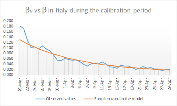
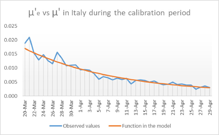
• 1.Neither the transmission rate $\beta$ nor the death rate ${\mu }^{\prime }$ due to COVID-19 are constant in our model. The available official data in the territories under study suggest that in the fist stages of the pandemic in territories with strict control on social distancing, both $\beta$ and ${\mu }^{\prime }$ decay exponentially (see for instance Figs. 2 and 3 ) to their baseline values ${\beta }_0$ and ${\mu }_0^{\prime }$ respectively. This is probably due to the fact that the evolution of the variables is still a transient and therefore some time is required until the parameters achieve their asymptotic values.
• 2.We consider a recuperation rate $\gamma$ which is not necessarily constant either. Although the observed values of $\gamma$ are somehow stable in the three countries under study, the monthly variations of $\gamma$ produce significant changes in the main epidemiological parameters. The way we chose the values of $\gamma$ is explained in the set of principles that provide the calibration of the model.
• 3.We consider the existence of a constant birth rate $\lambda >0$ which is the same for each of the three categories $S,$ $I$ and $R$. We also assume that all the descendants are born free of the infection, but without immunity.
• 4.Finally we consider the existence of a constant death rate $\mu >0$ due to death causes other than COVID-19.

Fig. 2.

Representation of ${\beta }_e\left(t\right)$ and $\beta \left(t\right)$ for Italy during the calibration period.

Fig. 3.

Representation of ${\mu }_e^{\prime }\left(t\right)$ and ${\mu }^{\prime }\left(t\right)$ for Italy during the calibration period.

The above assumptions produce the following relationship among the variables $S,I,R$:

$$\{\begin{array}{ccc}\hfill S^{\prime }& =& (\lambda -\mu )S+\lambda (I+R)-\beta SI,\hfill \\ \hfill I^{\prime }& =& \beta SI-\gamma I-{\mu }^{\prime }I-\mu I,\hfill \\ \hfill R^{\prime }& =& \gamma I-\mu R.\hfill \end{array}$$

The second set of hypotheses define the way the model must be calibrated, or in other words, how the parameters $\beta ,$ ${\mu }^{\prime },$ $\gamma ,$ $\lambda$ and $\mu$ are to be chosen:

• 1.The values of $\lambda$ and $\mu$ are provided in Table 1 .
• 2.As mentioned above, although the observed monthly mean values of the recuperation rate $\gamma$ are quite stable in all the territories under study it should not be taken for granted that $\gamma$ is necessarily constant. In principle, recuperation (or death) depends on human biological reaction to the virus. However, in a transient state variations on rates can be expected until asymptotic values are attained. This is precisely what seems to happend when one examines the data of Italy and the USA in connection with mortality and recuperation. We do assume, however, that $\gamma$ is constant along every calendar month or along the calibration period of every country. The values assigned to $\gamma$ are based on the average monthly observed values of $\gamma$. Normally the values of $\gamma$ are very uniform with quite a few exceptions, like the months of May and June in Italy, with values that are twice as big as in the rest of the months under study. The reasons that could explain this anomaly are far beyond the scope of this paper.
• 3.As for the determination of $\beta$ and ${\mu }^{\prime },$ we have observed a significant decay in the infection and death rate within the official data released by the authorities of the three countries under study. The functions $\beta$ and ${\mu }^{\prime }$ are defined using exponential regression on the official data. It must be said that according to real data, mortality approaches its asymptotic value in a relatively short period of time. This is compatible with the assumption that relevant changes, like new control policies or a sudden change in sociological behavior, may create a transient state where the parameters of the model may change until they approach their baseline values.

Table 1.

Normalized birth and death rates, $\lambda$ and $\mu$ respectively, of Italy, Spain and the USA measured in normalized births and deaths per day. All the data, including the total population $N,$ correspond to the year 2018.

Country	Birth rate $\lambda$	Death rate $\mu$	Population $N$
Italy	$1.992528\times {10}^{-5}$	$2.866523\times {10}^{-5}$	$6.05\times {10}^7$
Spain	$2.174293\times {10}^{-5}$	$2.494899\times {10}^{-5}$	$4.7\times {10}^7$
USA	$3.178082\times {10}^{-5}$	$2.356164\times {10}^{-5}$	$3.282\times {10}^8$

It is important to mention that we have run this model using the normalized variables:

$$\begin{array}{cc}\hfill S_N\left(t\right)& =S\left(t\right)/N,\hfill \\ \hfill I_N\left(t\right)& =I\left(t\right)/N,\hfill \\ \hfill R_N\left(t\right)& =R\left(t\right)/N,\hfill \end{array}$$

where $N=S+I+R$ is the total population. In this new variables the model would be

$$\{\begin{array}{ccc}\hfill S_N^{\prime }& =& (\lambda -\mu )S_N+\lambda (I_N+R_N)-\beta S_N{I}_N,\hfill \\ \hfill I_N^{\prime }& =& \beta S_N{I}_N-\gamma I_N-{\mu }^{\prime }{I}_N-\mu I_N,\hfill \\ \hfill R_N^{\prime }& =& \gamma I_N-\mu R_N,\hfill \end{array}$$ (1.2)

where the parameters $\lambda ,$ $\mu ,$ $\beta ,$ ${\mu }^{\prime }$ and $\gamma$ are all normalized.

Once $S_n\left(t\right),$ $I_N\left(t\right)$ and $R_N\left(t\right)$ are are obtained by numerical integration of (1.2), to recover the actual number of infected (active cases) $I\left(t\right)$ and the total number of recoveries $R\left(t\right),$ we have to multiply $I_N\left(t\right)$ and $R_N\left(t\right)$ by the total country’s population $N,$ i.e.,

$$\begin{array}{cc}\hfill I\left(t\right)& =N\left(t\right)·I_N\left(t\right),\hfill \\ \hfill R\left(t\right)& =N\left(t\right)·R_N\left(t\right).\hfill \end{array}$$

We assume that the initial population of the countries under study is the population they had in 2018. These data are shown in Table 1.

When the model is properly calibrated, its outcome for the variables $I$ and $R$ produce excellent approximations of the number of the reported number of active cases and people with immunity respectively. Additionally, other relevant parameters can also be accurately approximated. If we define

$$\begin{array}{cc}\hfill d\left(t\right)& ={\int }_{t-1}^t{\mu }^{\prime }\left(\xi \right)·I\left(\xi \right)d\xi ,\hfill \\ \hfill D\left(t\right)& ={\int }_0^t{\mu }^{\prime }\left(\xi \right)·I\left(\xi \right)d\xi ,\hfill \\ \hfill r\left(t\right)& ={\int }_{t-1}^t\gamma \left(\xi \right)·I\left(\xi \right)d\xi ,\hfill \\ \hfill i\left(t\right)& ={\int }_{t-1}^t\beta \left(\xi \right)·S\left(\xi \right)·I\left(\xi \right)d\xi ,\hfill \end{array}$$

then $d\left(t\right),$ $D\left(t\right),$ $i\left(t\right)$ and $r\left(t\right)$ are very sharp approximations of, respectively, the daily number of deaths, the aggregated number of deaths, the daily number of new infections and the daily number of recoveries on day $t$.

2. Calibrating the functions $\beta \left(t\right),$${\mu }^{\prime }\left(t\right)$ and $\gamma \left(t\right)$ during the first surge

First we describe the precise methodology used to find reasonably good approximations of the functions $\beta \left(t\right)$ and ${\mu }^{\prime }\left(t\right)$ for each of the territories considered in this paper. The approximation of these functions is done in two steps:

• 1.
  Firstly we calculate the daily infection and death rates using official data. If ${\beta }_e$ and ${\mu }_e^{\prime }$ are the empirical infection and death rates due to COVID-19, ${\beta }_e$ and ${\mu }_e^{\prime }$ are calculated using the following formulas:

  $$\begin{array}{cc}\hfill {\beta }_e(t+1)& =\frac{i_e(t+1)}{I_e\left(t\right)},\hfill \\ \hfill {\mu }_e^{\prime }(t+1)& =\frac{d_e(t+1)}{I_e\left(t\right)},\hfill \end{array}$$

  where $i_e\left(t\right)$ is the number of new reported infections on day $t,$ $d_e\left(t\right)$ is the number of new deaths reported on day $t$ and $I_e\left(t\right)$ is the number of reported active cases on day $t$. The aggregated number of deaths observed until day $t$ may be referred to later on as $D_e\left(t\right)$.
• 2.
  Secondly, once the empirical ${\beta }_e\left(t\right)$ and ${\mu }_e^{\prime }\left(t\right)$ are obtained, we have realized that ${\beta }_e$ and ${\mu }_e^{\prime }$ can be approximated fairly well by functions of the form:

  $$\begin{array}{cc}\hfill \beta \left(t\right)& ={\beta }_0+e^{a_{\beta }+b_{\beta }t},\hfill \\ \hfill {\mu }^{\prime }\left(t\right)& ={\mu }_0^{\prime }+e^{a_{{\mu }^{\prime }}+b_{{\mu }^{\prime }}t},\hfill \end{array}$$

  with $b_{\beta },b_{{\mu }^{\prime }}<0$. Therefore we are assuming that the parameters $\beta \left(t\right)$ and ${\mu }^{\prime }\left(t\right)$ decay exponentially to their baseline values ${\beta }_0$ and ${\mu }_0^{\prime }$ respectively. The values of $a_{\beta }$ and $b_{\beta }$ are calculated by using a linear regression scheme applied to the points

  $$(t,\log |{\beta }_e\left(t\right)-{\beta }_0\left|\right).$$

  Similarly, in order to obtain $a_{{\mu }^{\prime }}$ and $b_{{\mu }^{\prime }}$ we apply linear regression to the points

  $$(t,\log |{\mu }_e\left(t\right)-{\mu }_0^{\prime }\left|\right).$$

As for the determination of $\gamma ,$ we first calculate the daily recovery observed rates ${\gamma }_e\left(t\right),$ defined as

$${\gamma }_e(t+1)=\frac{r_e(t+1)}{I_e\left(t\right)},$$

where $r_e\left(t\right)$ represents the number of recoveries observed on day $t$. In order to calibrate the model in each of the countries under study we will assume that $\gamma$ is constant in every calendar month or along the calibration period of the functions $\beta \left(t\right)$ and ${\mu }^{\prime }\left(t\right)$. The values of $\gamma$ will be chosen in accordance with the mean values of the ${\gamma }_e\left(t\right)$’s.

2.1. Calibration of the model for the Italian case

The lockdown order was approved by the Italian Government on the $10th$ of March 2020. Our simulations for Italy start 10 days after the beginning of the lockdown, on the $20th$ of March. This day is day zero in all the graphs devoted to study the Italian case. We fist determine the infection and death rates on day $t,$ $\beta \left(t\right)$ and ${\mu }^{\prime }\left(t\right)$ respectively, using the daily number of reported new cases on day $t,$ $i_e\left(t\right),$ reported recoveries on day $t,$ $r_e\left(t\right),$ and reported deaths on day $t,$ $d_e\left(t\right)$. Recall that $I_e\left(t\right)$ is the reported amount of active cases at a given time $t$. Also, $R_e\left(t\right)$ and $D_e\left(t\right)$ represent, respectively, the total amount of reported recoveries and deaths until day $t$. As mentioned in Section 2, $\beta \left(t\right)$ is given by

$$\beta \left(t\right)={\beta }_0+e^{a_{\beta }+b_{\beta }t},$$

where, for a given choice of ${\beta }_0,$ $a_{\beta }$ and $b_{\beta }$ are calculated by linear regression applied to the points

$$(t,\log |{\beta }_e\left(t\right)-{\beta }_0\left|\right).$$

The values of ${\beta }_e\left(t\right)$ considered to calculate $a_{\beta }$ and $b_{\beta }$ have been imported from the internet using Excel and are based on the daily bulletins on the expansion of COVID-19 in Italy published by Protezione Civile [26]. The reader can find in Fig. 2 how $\beta \left(t\right)$ is compared to ${\beta }_e\left(t\right)$ for the choice ${\beta }_0=0.009$.

As for the calculation of ${\mu }^{\prime }\left(t\right),$ we have seen in Section 2 that ${\mu }^{\prime }\left(t\right)$ is given by

$${\mu }^{\prime }\left(t\right)={\mu }_0^{\prime }+e^{a_{{\mu }^{\prime }}+b_{{\mu }^{\prime }}t},$$

where, for a given choice of ${\mu }_0^{\prime },$ the values of $a_{{\mu }^{\prime }}$ and $b_{{\mu }^{\prime }}$ are calculated by linear regression applied to the points

$$(t,\log |{\mu }_e^{\prime }\left(t\right)-{\mu }_0^{\prime }\left|\right).$$

The values of ${\mu }_e^{\prime }\left(t\right)$ considered to calculate $a_{{\mu }^{\prime }}$ and $b_{{\mu }^{\prime }}$ have been taken from [26] as well. The reader can find in Fig. 3 how ${\mu }^{\prime }\left(t\right)$ is compared to ${\mu }_e^{\prime }\left(t\right)$ for the choice ${\mu }_0^{\prime }=0.0008$. The choice of ${\beta }_0$ and ${\mu }_0^{\prime }$ mentioned above, namely ${\beta }_0=0.015$ and ${\mu }_0^{\prime }=0.0008,$ minimizes the distance between ${\beta }_e$ and $\beta$ on the one hand, and between ${\mu }_e^{\prime }$ and ${\mu }^{\prime }$ on the other. Alternative choices of ${\beta }_0$ and ${\mu }_0^{\prime }$ produce predictions increasingly different from the reported data.

We know already how to obtain the functions $\beta \left(t\right)$ and ${\mu }^{\prime }\left(t\right),$ but in order to be able to run the model (1.2) we also need to know the parameters $\gamma ,$ $\lambda$ and $\mu$. The values of $\lambda$ and $\mu$ and the total country’s population $N$ are taken from Table 1.

To finish the calibration of the model in the Italian case we just need to determine $\gamma$. It turns out that the monthly average values of ${\gamma }_e\left(t\right)$ have stabilized since the end of July around 0.0160. However, during the first months of the pandemic in Italy the values of the ${\gamma }_e\left(t\right)$’s were bigger in general. We have considered the average values of the ${\gamma }_e\left(t\right)$’s in each of the periods pointed out in Table 2 .

Table 2.

Calibration of $\gamma$ for Italy. We consider the average values of the ${\gamma }_e\left(t\right)$’s in each period.

Period	Value considered for $\gamma$
Calibration period	0.0191
May	0.0375
June	0.0405
July	0.0233
From August onwards	0.0160

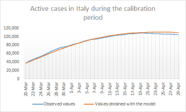
In order to asses the precision of the model, we have compared the reported active cases $I_e\left(t\right)$ and the model’s outcome for $I\left(t\right)$ during the 40-day calibration period in Fig. 4 .

Fig. 4.

Representation of the daily number of active cases in Italy $I_e\left(t\right)$ compared with the model’s outcome for $I\left(t\right)$ during the calibration period, from $20/03/2020$ to $29/04/2020$.

2.2. Calibration of the model for the Spanish case

The lockdown law was passed in the Spanish parliament on the $14th$ of March. The calibration period for Spain, as in the case of Italy, starts 10 days after the beginning of the lockdown, on the $24th$ of March. This day is day zero in all our graphs for the simulations about Spain. We fist approximate the infection and death rates $\beta \left(t\right)$ and ${\mu }^{\prime }\left(t\right)$ respectively using the daily number of reported new cases, $i_e\left(t\right),$ reported recoveries $r_e\left(t\right)$ and reported deaths $d_e\left(t\right)$.

Recall that $\beta \left(t\right)$ and ${\mu }^{\prime }\left(t\right)$ are given by

$$\begin{array}{ccc}\hfill \beta \left(t\right)& =& {\beta }_0+e^{a_{\beta }+b_{\beta }t}\text{and}\hfill \\ \hfill {\mu }^{\prime }\left(t\right)& =& {\mu }_0^{\prime }+e^{a_{{\mu }^{\prime }}+b_{{\mu }^{\prime }}t}\hfill \end{array}$$

respectively. For an appropriate choice of ${\beta }_0$ and ${\mu }_0^{\prime },$ the coefficients $a_{\beta },$ $b_{\beta },$ $a_{{\mu }^{\prime }}$ and $b_{{\mu }^{\prime }}$ are calculated by linear regression applied to the points

$$(t,\log |{\beta }_e\left(t\right)-{\beta }_0\left|\right)\text{and}(t,\log |{\mu }_e^{\prime }\left(t\right)-{\mu }_0^{\prime }\left|\right).$$

The values of ${\beta }_e\left(t\right)$ used to calculate the coefficients have been imported from the internet using Excel, and are based on the data published by the Instituto de Salud Carlos III (ISCIII, Madrid, Spain), [27], and the University Johns Hopkins [28]. The optimal choice of ${\beta }_0$ and ${\mu }_0^{\prime }$ is ${\beta }_0=0.015$ and ${\mu }_0^{\prime }=0.00055$.

On the other hand, the value we have assigned to $\gamma$ is the average of the ${\gamma }_e\left(t\right)$’s since the 24th of March until the 18th of May. It is important to mention that Spain does not publish the number of daily recoveries since the 18th of May 2020, for which reason right now we cannot have an idea about how many active cases there are in the country.

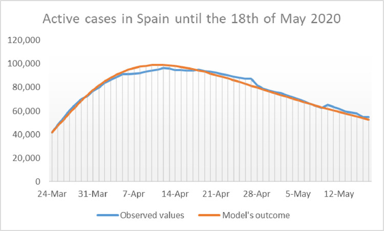
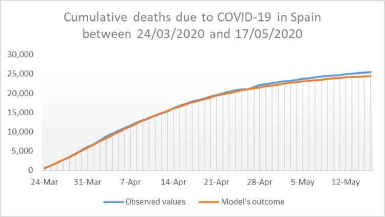
Once we have $\beta \left(t\right)$ and ${\mu }^{\prime }\left(t\right)$ for Spain for a given choice of ${\beta }_0$ and ${\mu }_0^{\prime },$ we perform a 37 day simulation of the model and compare the outcome with the reported data. The calibration is complete by putting $\gamma =0.0357,$ which is the average of ${\gamma }_e\left(t\right)$ over the 37 days of the calibration period. The reader can asses the accuracy of the model with the calibration mentioned above by taking a look at Figs. 5 and 6 , where the outcome of the calibrated model for $I\left(t\right)$ and $D\left(t\right)$ appear in the same picture as the reported data of active cases, $I_e\left(t\right)$ and cumulative deaths, $D_e\left(t\right),$ respectively. Observe that here cumulative deaths are counted since the 24th of March, and not since the beginning of the pandemic.

Fig. 5.

Representation of the daily number of reported active cases in Spain $I_e\left(t\right)$ compared with the model’s outcome $I\left(t\right)$.

Fig. 6.

Representation of the deaths by COVID-19 in Spain from March 24th until May 17th, 2020. Here $D_e\left(t\right)$ appears in blue whereas $D\left(t\right)$ is shown in red. (For interpretation of the references to color in this figure legend, the reader is referred to the web version of this article.)

2.3. Calibration of the model for the USA

As in the previous two cases we calculate the best fit for ${\beta }_e\left(t\right)$ and ${\mu }_e^{\prime }\left(t\right)$ by means of exponentials using a linear regression scheme. The data we have used in this case range from the $2nd$ of April to the 2nd of May. The reasons why we have started on April $2nd$ are similar to the arguments that led us to the initial dates for Italy and Spain, i.e., most of the states in the US began their stay-at-home policies about ten days before April 2. The data, as in the Italian and Spanish cases, were downloaded from tables in the internet using Excel and are based on the data provided by the Johns Hopkins University in its COVID-19 web page [28]. The optimal choice for ${\beta }_0$ and ${\mu }_0^{\prime }$ is ${\beta }_0=0.0165$ and ${\mu }_0^{\prime }=0.00032.$ As for the calibration of $\gamma ,$ we have noticed that the average monthly values of the ${\gamma }_e\left(t\right)$’s are not as homogeneous as in Italy. The values we have considered for $\gamma$ can be seen in Table 3 .

Table 3.

Calibration of $\gamma$ for the USA.

Period	Value considered for $\gamma$
April	0.0090
May	0.0160
June	0.0165
July	0.0185
August	0.0165
September	0.0160
October	0.0190
November	0.0200

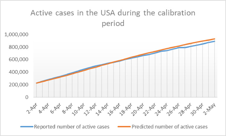
In order to check the accuracy of the calibration described above, the reader is invited to take a look at Fig. 7 , where the model’s outcome for $I\left(t\right)$ and the observed active cases $I_e\left(t\right)$ are shown in the same graph during the calibration period.

Fig. 7.

Representation of the daily number of reported active cases in the USA $I_e\left(t\right)$ compared with $I\left(t\right)$ during the calibration period.

3. Behavior of the model during the first and successive surges of COVID-19

In this section we examine the course of the pandemic of COVID-19 using the model defined and calibrated in the previous sections. In the absence of any significant change with respect to the conditions that held in calibration period, the course of COVID-19 would be controlled by the parameters $\beta \left(t\right),$ ${\mu }^{\prime }\left(t\right)$ and the constant value of $\gamma$ determined during the calibration period. However, several significant events took place at the end of the calibration period in each of the countries under study, including the relaxation or even the end of the lock down, that contributed to increase the number of contacts and the probability that a contact results in an infection. In Spain, for instance, people were allowed to walk within 1.5 kilometers from their homes in May, bars and restaurants were allowed to reopen in many regions of the country along June, and in July, internal mobility was allowed with no restrictions, giving birth to a period called “new normality”.

All the changes mentioned in the previous paragraph do not seem to have exerted any influence on mortality, but they did help to raise the transmission of the virus. For this reason, in order to model the second (or third) surge we will need to adapt the transmission function $\beta \left(t\right)$ at some stage. The rest of the parameters needed to run the model remain as they have been defined already. The new transmission function will be denoted by ${\beta }^{*}\left(t\right)$.

It is arguable whether environmental conditions could exert a relevant influence on the course of COVID-19. The effects of temperatures and relative humidity on the coronavirus survival on surfaces and in the air has been studied in the past (see for instance [29]). More recent studies predict a negative impact of hot weather, combined with a certain degree of humidity, in the ability of the virus to spread and infect (see for instance [30]). The fact that other diseases produced by a coronavirus, like the SARS of $2002-2003,$ reached its peak in May and disappeared from the Northern Hemisphere during the Summer, should have not misguided our response to the virus along the months of June and July, and in lesser level in August too (see for instance [31]). Actually, signs of a second surge of the pandemic of COVID-19 could be observed in Europe and the USA already during the months of June and July 2020, when the weather is quite hot in some countries, like Italy and Spain, or in many areas of the USA. The reasons that explain this second surge could be sociological, and are probably related to a substantial increasement of the population’s mobility due to Summer holidays accompanied by a relaxation of the social distancing measures. All these changes affect the transmissibility of the virus. What we do in this section is to propose a model of transmission function in each of the countries under study which is compatible with real transmissibility data during the second (or third) surge. Once we have an appropriate candidate for the transmission function, the application of our model produces reasonable outcomes about other epidemiological parameters, such as daily new cases, daily and cumulative deaths, to mention just a few. In most cases, the model’s outcomes and real epidemiological data almost coincide.

3.1. Evolution of the first and second surge of Covid-19 in Italy

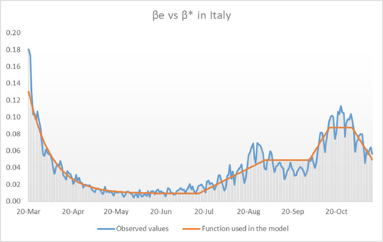
In the case of Italy we can observe a slight but steady growth of the values of ${\beta }_e\left(t\right)$ since the month of July (see blue graph in Fig. 8 ).

Fig. 8.

Comparison of the transmission function ${\beta }^{*}\left(t\right)$ used in the model and the observed values of ${\beta }_e\left(t\right)$ until mid November 2020.

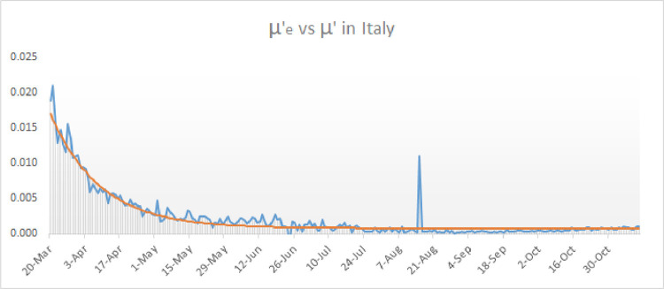
Unlike what happends with the ${\beta }_e\left(t\right)$’s, the values of ${\mu }_e^{\prime }\left(t\right)$ seem to have a much more predictable behavior as can be seen in Fig. 9 . Hence, in order to simulate the second surge of COVID-19 in Italy we can assume that ${\mu }^{\prime }\left(t\right)$ has already approximated to its baseline value ${\mu }_0^{\prime }$ since the month July and on, whereas $\beta$ must be reshaped starting from the month of July according to the values of ${\beta }_e\left(t\right)$.

Fig. 9.

Comparison of the death rate function ${\mu }^{\prime }\left(t\right)$ used in the model and the observed values of ${\beta }_e\left(t\right)$ until mid November 2020.

Actually, we will replace $\beta \left(t\right)$ by ${\beta }^{*}\left(t\right),$ where ${\beta }^{*}\left(t\right)$ is shown in red in Fig. 8. Observe that $\beta \left(t\right)$ and ${\beta }^{*}\left(t\right)$ coincide until mid July. To be more precise, until the 16th of July ($t=117$). The function ${\beta }^{*}\left(t\right)$ we have considered to model the second surge in Italy is given explicitly by

$${\beta }^{*}\left(t\right)=\{\begin{array}{cc}\beta \left(t\right)\hfill & \text{if}t\le 117,\hfill \\ \beta \left(117\right)+\frac{5.5{\beta }_0-\beta \left(117\right)}{30}(t-117)\hfill & \text{if}117\le t\le 164,\hfill \\ 5.5{\beta }_0\hfill & \text{if}164\le t\le 195,\hfill \\ 5.5{\beta }_0+\frac{4.5{\beta }_0}{15}(t-195)\hfill & \text{if}195\le t\le 210,\hfill \\ 10{\beta }_0\hfill & \text{if}210\le t\le 225,\hfill \\ 10{\beta }_0-\frac{4.5{\beta }_0}{15}(t-225)\hfill & \text{if}225\le t\le 240.\hfill \end{array}$$

Observe that $t=117,164,195,210,225,240$ correspond, respectively, to the 16th of July, the 31st of August, the 1st of October, the 16th of October, the 31st of October and the 15th of november. The function ${\beta }^{*}\left(t\right)$ is depicted in Fig. 8 in red, together with ${\beta }_e\left(t\right)$.

The accuracy of the model’s outcomes with $\beta \left(t\right)$ replaced by ${\beta }^{*}\left(t\right)$ is shown Figs. 10 and 11 .

Fig. 10.

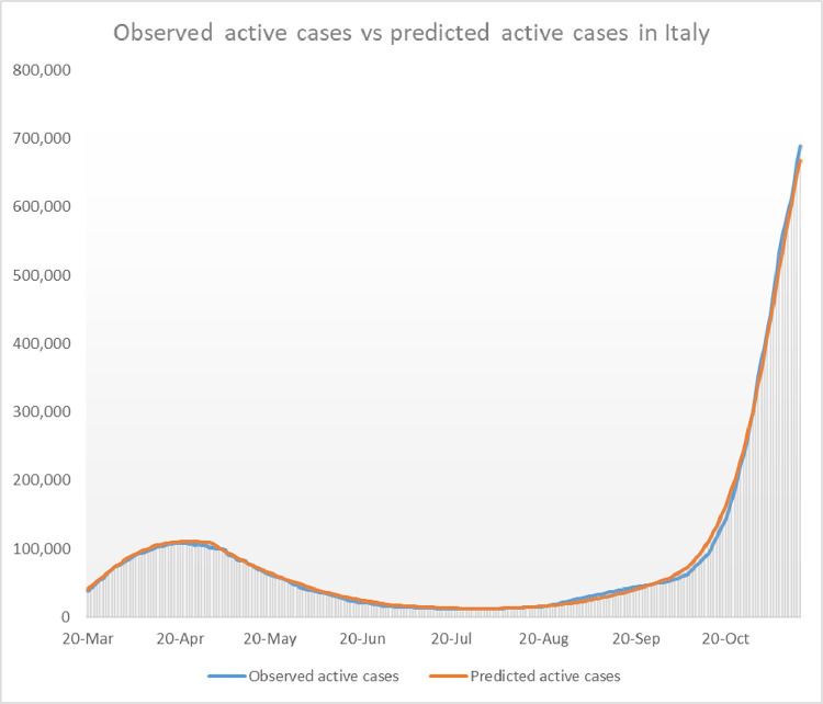
Comparison of the model’s outcome for $I\left(t\right)$ and the observed values $I_e\left(t\right)$ of active cases in Italy until mid november 2020.

Fig. 11.

In the left we show the number of deaths by COVID-19 in Italy since the 20th of march compared with the deaths predicted by the model. On the right we compare the observed cumulative incidence in 14 days per 100,000 inhabitants in Italy since mid August with the values predicted by our model.

3.2. Evolution of the second and third surge of COVID-19 in the USA

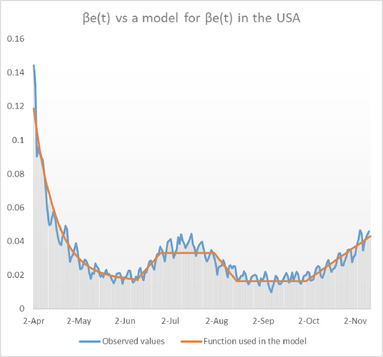
The USA already suffered a second bust of COVID-19 in Summertime that manifested with a substancial increasement of deaths in August with respect to June and July. However this second surge had its origin a few weeks earlier in the month of July, as can be seen in Fig. 12 . Observe the heap in the graph of ${\beta }_e\left(t\right)$ along the month of July, when the transmission was multiplied by 2. It seems that the ${\beta }_e\left(t\right)$’s decreased in August and stabilized around the baseline value ${\beta }_0$ in September. Unfortunately, since the beginning of October, the values of the ${\beta }_e\left(t\right)$’s have experienced a dramatic rise, giving birth to the third surge of COVID-19 in the USA. The transmission function ${\beta }^{*}\left(t\right)$ we have used to model the second and third surge in the USA is shown in red in Fig. 12. We provide it explicitly here:

$${\beta }^{*}\left(t\right)=\{\begin{array}{cc}\beta \left(t\right)\hfill & \text{if}t\le 69,\hfill \\ \beta \left(169\right)+\frac{2{\beta }_0-\beta \left(69\right)}{15}\hfill & \text{if}69\le t\le 84,\hfill \\ 2{\beta }_0\hfill & \text{if}84\le t\le 120,\hfill \\ 2{\beta }_0-\frac{{\beta }_0}{15}(t-120)\hfill & \text{if}120\le t\le 135,\hfill \\ {\beta }_0\hfill & \text{if}135\le t\le 182\hfill \\ {\beta }_0+\frac{1.5{\beta }_0}{40}(t-182)\hfill & \text{if}182\le t\le 227.\hfill \end{array}$$

Observe that $t=69,84,120,135,182,220$ correspond, respectively, to the 10th of June, the 25th of June, the 31st of July, the 15th of August, the 1st of October and the 8th of November.

Fig. 12.

Comparison of the transmission function $\beta \left(t\right)$ used in the model and the observed values of ${\beta }_e\left(t\right)$ until mid November 2020 in the USA.

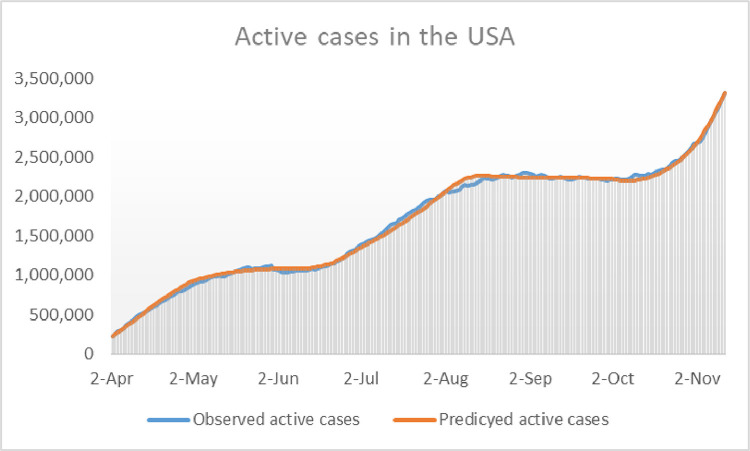
The results obtained with this choice of ${\beta }^{*}\left(t\right)$ model with great accuracy the main epidemiological figures of the USA during the second and third surge. To provide the reader with some examples of the sharpness and precision of our model, see Figs. 13 and 14 .

Fig. 13.

Comparison of the model’s outcome for $I\left(t\right)$ and the observed values $I_e\left(t\right)$ of active cases in the USA until mid november 2020.

Fig. 14.

In the left we show the number of deaths by COVID-19 in the USA since the 2nd of April compared with the deaths predicted by the model. On the right we the cumulative number of reported recoveries together with the model’s outcome for $R\left(t\right)$. The difference between the two graphs is due to the deaths of recoveries for causes other than COVID-19.

3.3. Evolution of the second and third surge of COVID-19 in Spain

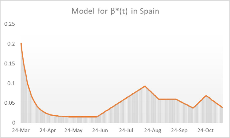
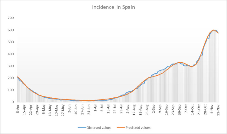
The fact that Spain does not publish the number of daily recoveries since the 18th of May 2020 hampers considerably the construction of a model for the transmission function ${\beta }^{*}\left(t\right)$ during the second surge in that country since we are unable to calculate the values of ${\beta }_e\left(t\right)$. Using a heuristic procedure, we have found a function ${\beta }^{*}\left(t\right)$ such that the model’s outcome and the real data for the cumulative incidence per 100,000 inhabitants coincide. Consider the function (see Fig. 15 ) defined as

$${\beta }^{*}\left(t\right)=\{\begin{array}{cc}\beta \left(t\right)\hfill & \text{if}t\le 89,\hfill \\ \beta \left(89\right)+\frac{6.2{\beta }_0-\beta \left(89\right)}{56}(t-89)\hfill & \text{if}89\le t\le 145,\hfill \\ 6.2{\beta }_0-\frac{2.2{\beta }_0}{16}(t-145)\hfill & \text{if}145\le t\le 161,\hfill \\ 4{\beta }_0\hfill & \text{if}161\le t\le 181,\hfill \\ 4{\beta }_0-\frac{1.5{\beta }_0}{20}(t-181)\hfill & \text{if}181\le t\le 201,\hfill \\ 2.5{\beta }_0+\frac{2.1{\beta }_0}{15}(t-201)\hfill & \text{if}201\le t\le 216,\hfill \\ 4.6{\beta }_0-\frac{2.1{\beta }_0}{20}(t-216)\hfill & \text{if}216\le t\le 236.\hfill \end{array}$$

Observe that $t=89,145,161,181,201,216,236$ correspond, respectively, to the 21st of June, the 16th of August, the 1st of September, the 21st of September, the 11th of October, the 26th of October and the 15th of November. Running the model with ${\beta }^{*}\left(t\right),$ the outcome for cumulative incidence in 14 days per 100,000 inhabitants and the real reported incidence have been sketched in Fig. 16 .

Fig. 15.

Heuristic construction of the transmission function ${\beta }^{*}\left(t\right)$ for Spain during the second surge.

Fig. 16.

We show the cumulative incidence in 14 days per 100,000 inhabitants in Spain obtained with our model compared with real cumulative incidence data.

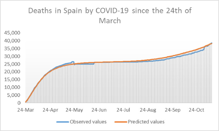
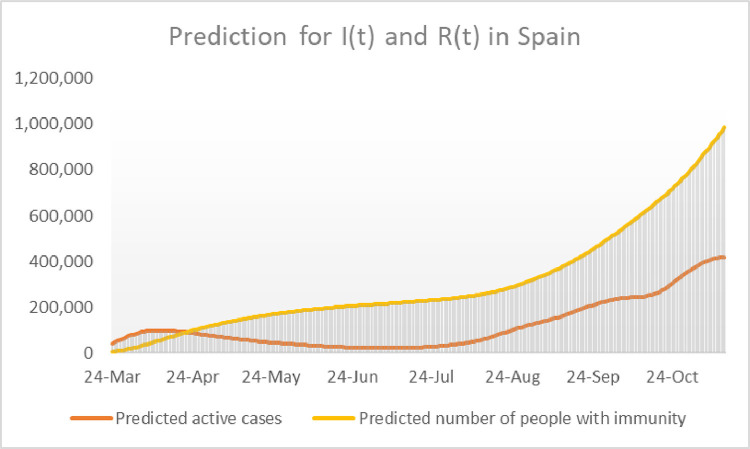
The fact that the graphs in Fig. 17 , are similar, proves that the choice made for ${\beta }^{*}\left(t\right)$ could be appropriate to model the course of the pandemic in Spain during the second surge. Using the function ${\beta }^{*}\left(t\right)$ it is therefore plausible to make an educated guess of the evolution of active cases and the number of people with immunity by representing the model’s outcome for $I\left(t\right)$ and $R\left(t\right)$ respectively. We do that in Fig. 18 .

Fig. 17.

Real data of cumulative deaths by COVID-19 are compared with the model outcome for cumulative deaths since the 24th of March.

Fig. 18.

Estimated values of active cases and people with immunity in Spain between the 24th of March and mid November 2020.

It must be warned that the graphs in Fig. 18, together with the heuristic guess for ${\beta }^{*}\left(t\right)$ have been obtained under the assumption that $\gamma$ remains constant along the whole period of study. Also, the value assigned to $\gamma$ has been estimated using only the data of the fist weeks of the pandemic. This value, namely $\gamma =0.0357,$ seems to be a bit high in comparison with the recuperation rates of Italy and the USA, which seem to have stabilized within the relatively narrow interval [0.016,0.020]. There are no objective reasons to explain why the recuperation constant in Spain should be about twice as big as in Italy or the USA, for which reason we tend to believe that the current number of active cases in Spain could be higher than the predicted values shown in Fig. 18.

4. Predictions for Italy and the USA

To finish this manuscript we will provide some projections on the evolution of COVID-19 in the countries under study using the model described in the preceding sections. Out of the three countries, we believe that Italy has published the most homogeneous, consistent and reliable data, so predictions could be more accurate in this case. On the contrary, the data of Spain have undergone substantial corrections along the pandemic and they lack reliable figures on recovered people since the month of may. For this reason we will restrict our attention to Italy and the USA.

4.1. Projections for Italy

If we examine the data of Italy by mid November, we can see that new infections, cumulative incidence, daily deaths and other epidemiological indicators are still growing or stabilized around very high values. However, the transmission curve ${\beta }_e\left(t\right)$ for Italy (see Fig. 8) has been decreasing since the beginning of November. This descending tendency will surely translate into a steady reduction of the most significant epidemiological figures in the next few weeks starting on the 16th of November 2020 $t=241,$ when the revision of this paper has been finished. To obtain our projections for Italy we will consider the same function ${\mu }^{\prime }\left(t\right)$ (which at that stage will be almost equal to ${\mu }_0^{\prime }$), but the function ${\beta }^{*}\left(t\right)$ will be extended for $t\ge 241$ as follows:

$${\beta }^{*}\left(t\right)=\{\begin{array}{cc}10{\beta }_0-\frac{4.5{\beta }_0}{15}(t-225)\hfill & \text{if}225\le t\le 255,\hfill \\ {\beta }_0\hfill & \text{if}t\ge 255.\hfill \end{array}$$

Observe that $t=225$ is the 15th of November whereas $t=255$ is the 30th of November.

The model’s outcome for daily deaths and cumulative incidence in 14 days per 100,000 inhabitants can be seen in Fig. 19 in two different scenarios. In the worst scenario we assume that the recuperation constant $\gamma$ preserves the value it had since the month of August, that is $\gamma =0.0160$. In the optimist scenario $\gamma$ is supposed to have the value it had in June, that is $\gamma =0.0405$. It is devastating that, in the worst scenario, the incidence will not fall below the threshold of 50 cases until mid April 2020, and by that time some 62,000 people could have died since the 16th of November alone. In the most favorable scenario, the cumulative incidence would fall below 50 cases right at the beginning of 2021. In this scenario about 16,000 people would die between the 16th of November and the end of 2020 and about 4,700 mode in 2021. Daily deaths would not fall below 10 until the end of March 2021. Daily new cases would not fall below 50 untl mid April 2021.

Fig. 19.

On the left we show a projection on the daily number of deaths in Italy starting in mid November. On the right we show a projection on the cumulative incidence in 14 days per 100,000 inhabitants in Italy. In all cases the projections star in mid November 2020.

4.2. Projections for the USA

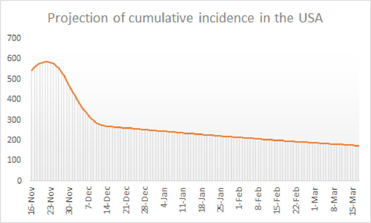
Looking at the transmission curve of the USA (see Fig. 12) it seems that the third surge is still on the rise with no sign of change by mid November 2020 when the revision of this paper has been concluded. Even in the case that a dramatic change of tendency occurs in mid November with a linear decay of ${\beta }^{*}\left(t\right)$ to the base line value ${\beta }_0$ in, say, 15 days, the situation would be quite bad with at least 1,000 deaths every day until the end of January 2021. To calculate our projections, let us extend ${\beta }^{*}\left(t\right)$ as follows:

$${\beta }^{*}\left(t\right)=\{\begin{array}{cc}\frac{43}{16}{\beta }_0-\frac{9{\beta }_0}{80}(t-227)\hfill & \text{if}227\le t\le 242,\hfill \\ {\beta }_0\hfill & \text{if}t\ge 260.\hfill \end{array}$$

Here $t=227$ is the 16th of November and $t=242$ is the 30th of November. With this transmission function the pandemic would be quite spread in the USA for several months, having very high incidence values way above 100 cases even in the month of March 2021 (see Fig. 20 ).

Fig. 20.

Projected cumulative incidence in 14 days per 100,000 inhabitants in the USA.

5. Conclusions and discussion

In this paper we have seen that the course of COVID-19 in three countries, Italy, Spain and the USA, can be modeled using a simple SIR-type model with non-constant parameters. The parameters, after a transient state tend to approach their asymptotic values. This is particularly true with the mortality rate ${\mu }^{\prime }$ and the recuperation rate. The transmission rate shows a tendency to approach its asymptotic value as well, but it is sensitive to sociological changes such as a higher mobility, a relaxation of social distancing and the massive use of protection material, like face masks. We have proved that an appropriate choice of the transmission function allows us to obtain very realistic outcomes. Using the model, we have also been able to produce several predictions in the case of Italy and the USA. These predictions a quite negative even in the most favorable scenario, which should serve as a motivation to double the efforts of everybody. The situation of the USA is so bad that, even if the current tendency is reversed in just two weeks, that country would keep extremely high values of incidence even in the month of March 2021. Only a dramatic fall of the transmission, even below its baseline value, could bring some normality to that country. In any case, that would not happend immediately.

Declaration of Competing Interest

The authors declare that they have no known competing financial interests or personal relationships that could have appeared to influence the work reported in this paper.

References

- 1.Lajmanovich A., Yorke J.A. A deterministic model for gonorrhea in a nonhomogeneous population. Math Biosci. 1976;28(3-4):221–236. [Google Scholar]
- 2.Rapatski B.L., Suppe F., Yorke J.A. HIV epidemics driven by late disease stage transmission. J Acquir Immune Defic Syndr. 2005;38(241) [PubMed] [Google Scholar]
- 3.Riley S. Transmission dynamics of the etiological agent of SARS in Hong Kong: impact of public health interventions. Science. 2003;300(1961) doi: 10.1126/science.1086478. [DOI] [PubMed] [Google Scholar]
- 4.Osemwinyen A., Diakhaby A. Mathematical modelling of the transmission dynamics of Ebola virus. Appl Comput Math. 2015;4(313) [Google Scholar]
- 5.Ferguson N.M., Cummings D.A.T., Fraser C., Cajka J.C., Cooley P.C., Burke D.S. Strategies for mitigating an influenza pandemic. Nature. 2006;442(448) doi: 10.1038/nature04795. [DOI] [PMC free article] [PubMed] [Google Scholar]
- 6.Anderson R.M., May R.M. Oxford University Press; Oxford: 1991. Infectious diseases un humans: dynamics and control. [Google Scholar]
- 7.Hadeler K.P. Lecture notes on mathematical modelling in the life sciences. Springer; Cham: 2017. Topics in mathematical biology. [Google Scholar]; Xiv+353 pp
- 8.Inaba H. Springer; Singapore: 2017. Age-structured population dynamics in demography and epidemiology. [Google Scholar]; Xix+555
- 9.Martcheva M. Texts in applied mathematics. vol. 61. Springer; New York: 2015. An introduction to mathematical epidemiology. [Google Scholar]; Xiv+453 pp
- 10.Diekmann O., Heesterbeek H., Britton T. Princeton University Press; Princeton, NJ: 2013. Mathematical tools for understanding infectious disease dynamics. (Princeton series in theoretical and computational biology). [Google Scholar]; Xiv+502 pp
- 11.Thieme H. Princeton University Press; Princeton, NJ: 2003. Mathematics in population biology. (Princeton Series in Theoretical and Computational Biology). [Google Scholar]; Xx+543 pp.
- 12.Brauer F., Castillo-Chavez C., Feng Z. Texts in applied mathematics. vol. 69. Springer; New York: 2019. Mathematical models in epidemiology. [Google Scholar]
- 13.May R.M. Simple mathematical models with very complicated dynamics. Nature. 1976;261(459) doi: 10.1038/261459a0. [DOI] [PubMed] [Google Scholar]
- 14.Kermack W.O., McKendrick A.G. A contribution to the mathematical theory of epidemics. Proc R Soc A. 1927;115(700) doi: 10.1007/BF02464423. [DOI] [PubMed] [Google Scholar]
- 15.Harko T., Lobo F.S.N., Mak M.K. Exact analytical solutions of the susceptible-infected-recovered (SIR) epidemic model and of the SIR model with equal death and birth rates. Appl Math Comput. 2014;236(184) [Google Scholar]
- 16.Wu F. A new coronavirus associated with human respiratory disease in China. Nature. 2020;579(265) doi: 10.1038/s41586-020-2008-3. [DOI] [PMC free article] [PubMed] [Google Scholar]
- 17.Lin Q. A conceptual model for the coronavirus disease 2019 (COVID-19) outbreak in Wuhan, China with individual reaction and governmental action. Int J Infect Dis. 2020;93(211) doi: 10.1016/j.ijid.2020.02.058. [DOI] [PMC free article] [PubMed] [Google Scholar]
- 18.Guan W. Early transmission dynamics in Wuhan, China, of novel coronavirus-infected pneumonia. N Engl J Med. 2020;382(1199) doi: 10.1056/NEJMoa2001316. [DOI] [PMC free article] [PubMed] [Google Scholar]
- 19.Zhu N. for the China medical treatment expert group for COVID-19, clinical characteristics of coronavirus disease 2019 in China. N Engl J Med. 2020;382(727) doi: 10.1056/NEJMoa2002032. [DOI] [PMC free article] [PubMed] [Google Scholar]
- 20.Ivorra B., Ferrández M.R., Vela-Pérez M., Ramos A.M. Mathematical modeling of the spread of the coronavirus disease 2019 (COVID-19) taking into account the undetected infections. The case of China. Commun Nonlinear Sci Numer Simul. 2020;88(105303) doi: 10.1016/j.cnsns.2020.105303. [DOI] [PMC free article] [PubMed] [Google Scholar]
- 21.Manchein C., Brugnago E.L., Silva R.M.d., Mendes C.F.O., Beims M.W. Strong correlations between power-law growth of COVID-19 in four continents and the inefficiency of soft quarantine strategies. Chaos. 2020;30(041102) doi: 10.1063/5.0009454. [DOI] [PMC free article] [PubMed] [Google Scholar]
- 22.Anderson R., May R. Population biology of infectious diseases: Part I. Nature. 1979;280:361–367. doi: 10.1038/280361a0. [DOI] [PubMed] [Google Scholar]
- 23.Hadeler K.P., Dietz K., Safan M. Case fatality models for epidemics in growing populations. Math Biosci. 2016;281:120–127. doi: 10.1016/j.mbs.2016.09.007. [DOI] [PubMed] [Google Scholar]
- 24.Thieme H. Epidemic and demographic interaction in the spread of potentially fatal diseases in growing populations. Math Biosci. 1992;111:99–130. doi: 10.1016/0025-5564(92)90081-7. [DOI] [PubMed] [Google Scholar]
- 25.Lina Q., Zhaob S., Gaod D., Loue Y., Yangf S., Musae S.S., et al. A conceptual model for the coronavirus disease 2019 (COVID-19) outbreak in Wuhan, China with individual reaction and governmental action. Int J Infect Dis. 2020;93:21116. doi: 10.1016/j.ijid.2020.02.058. [DOI] [PMC free article] [PubMed] [Google Scholar]
- 26.Organization. Protezione Civile Italia. Daily bulletins on the state of the infections in Italy. http://www.protezionecivile.gov.it/web/guest/media-communication/press-release.
- 27.Organization. Instituto de Salud Carlos III. Daily reports on the state of the expansion of COVID 19 in Spain:. https://www.isciii.es/QueHacemos/Servicios/VigilanciaSaludPublicaRENAVE/EnfermedadesTransmisibles/Paginas/InformesCOVID-19.aspx.
- 28.Organization. Johns Hopkins University. coronavirus resource center. https://coronavirus.jhu.edu/.
- 29.Casanova L.M., Jeon S., Rutala W.A., Weber D.J., Sobsey M.D. Effects of air temperature and relative humidity on coronavirus survival on surfaces. Appl Environ Microbiol. 2010;76(9):2712–2717. doi: 10.1128/AEM.02291-09. [DOI] [PMC free article] [PubMed] [Google Scholar]
- 30.Wang J., Tang K., Feng K., Lv W.. High temperature and high humidity reduce the transmission of COVID-19March 9, 2020. Available at SSRN: https://ssrn.com/abstract=3551767.
- 31.Carlson C.J., Gomez A.C.R., Bansal S., et al. Misconceptions about weather and seasonality must not misguide COVID-19 response. Nat Commun. 2020;11(4312) doi: 10.1038/s41467-020-18150-z. [DOI] [PMC free article] [PubMed] [Google Scholar]