On the analysis of number of deaths due to Covid −19 outbreak data using a new class of distributions

Abstract

In this article, we develop a generator to suggest a generalization of the Gumbel type-II model known as generalized log-exponential transformation of Gumbel Type-II (GLET-GTII), which extends a more flexible model for modeling life data. Owing to basic transformation containing an extra parameter, every existing lifetime model can be made more flexible with suggested development. Some specific statistical attributes of the GLET-GTII are investigated, such as quantiles, uncertainty measures, survival function, moments, reliability, and hazard function etc. We describe two methods of parametric estimations of GLET-GTII discussed by using maximum likelihood estimators and Bayesian paradigm. The Monte Carlo simulation analysis shows that estimators are consistent. Two real life implementations are performed to scrutinize the suitability of our current strategy. These real life data is related to Infectious diseases (COVID-19). These applications identify that by using the current approach, our proposed model outperforms than other well known existing models available in the literature.

Introduction

Lifetime phenomenon modeling and interpretation is an important component of statistical research in a broad variety of scientific and technical fields. The study of lifetime data analysis has developed rapidly and expanded in terms of methodology, theory, and application fields. Continuous distributions of probabilities and other methods of generalization or transformation have been introduced in the framework of characterising real life events. Such generalizations derived either by incorporating one or more than one shape parameters, or by adjusting distribution’s functional form, improve model flexibility and model the phenomena more precisely. Extensive software innovations made less emphasis on computational details and thus simplified estimation methods.

The below are popular and frequently referenced transformations presented during recent past in statistical studies for characterizing real life models. Marshal and Olkin [1] transform survival function by putting an additional parameter. Gupta et al. [2] introduced the exponentiated family of models by adding the extra shape parameter like an exponent to basic cdf. Beta-generated family by Eugene et al. [3] focused on Beta type-I and II models. On the other side, Kumaraswamy-generated family by Cordeiro and Castro [4] prefers the Kumaraswamy model instead of the Beta model. Zografos and Balakrishnan [5] introduced a versatile gamma-G class of models focused on GG (Generalized Gamma) model.

Here, our goal is to suggest a novel class of model that accommodates different kinds of hazard rates for suitable selection of shape parameter. The transformation of generalized logarithmic exponential is suggested on Gumbel type-II cdf, hereafter referred as Generalized log-exponential (GLE) transformation. The model, thus produced, is supposed to have both monotone and upside bathtub shaped hazard rates and based on the selection of parametric values. Let Y is a random variable (r.v.) with cdf and pdf ($G\left(y\right),g\left(y\right)$ respectively) taken as baseline model.

$$F\left(y\right)=\frac{\log \left\{2-e^{-\xi {\left(G\left(y\right)\right)}^{\lambda }}\right\}}{\log \left\{2-e^{-\xi }\right\}}\text{;}\lambda >0,$$ (1)

with

$$f\left(y\right)=\frac{\xi \lambda e^{-\xi {\left(G\left(y\right)\right)}^{\lambda }}g\left(y\right){\left\{G\left(y\right)\right\}}^{\lambda -1}}{\log \left\{2-e^{-\xi }\right\}\left(2-e^{-\xi {\left(G\left(y\right)\right)}^{\lambda }}\right)}\text{;}\lambda >0\text{.}$$ (2)

Motivated from [6], who taken into account less flexible transformation. Whereas their approach allows only fixed modulation of shape of distributions, our approach is more versatile because it incorporates additional shape parameter. To explain our perspective, we consider Gumbel type-II [7], [8], [9], [10], [11] as base model due to its simplicity and usability in life testing problem. Our proposed model known as generalized log-exponential transformation of Gumbel Type-II (GLET-GTII), which extends a more flexible model for modeling life data.

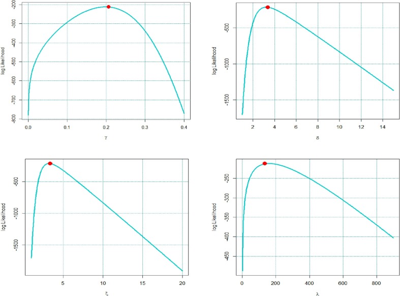
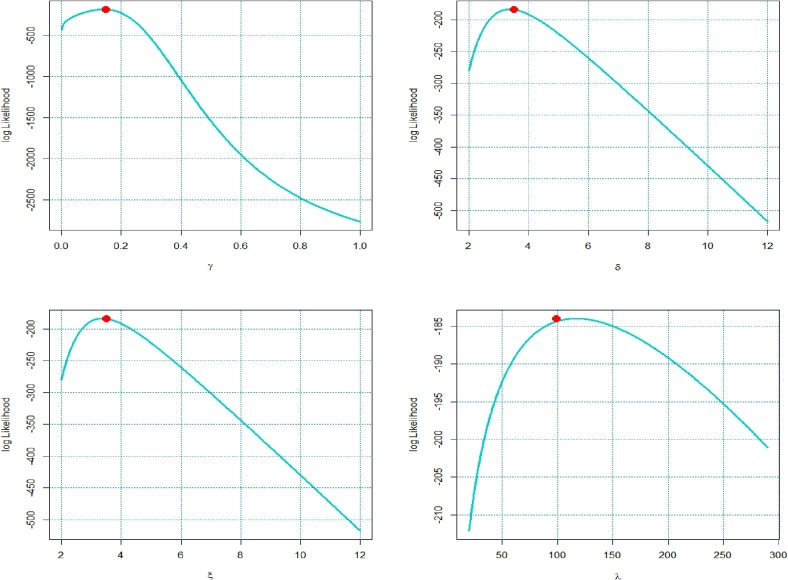
Infectious diseases are disorders induced by organisms, like viruses, parasites, bacteria, fungi etc. A lot of species are living in and on our bodies. Normally, they are harmless, or some times they are helpful. In certain conditions, however, some organisms may cause illness. However, under certain scenarios, some organisms may develop disease. Some infectious diseases can be transferred from one person to another. Some are disseminated by bugs or other animals. And one may have others by eating tainted water or food or being exposed to toxic organisms. Intimations and symptoms change widely depending on microbes resulting infection, but commonly involve fatigue and fever. Slight infections can lead to relax and home medication, while some life-threatening infections may require hospitalization. Certain infectious diseases, like measles, pneumonia and chickenpox, can be restrained using vaccinations. Regular and detailed hand-washing also succours protect you from certain infectious diseases. Only minor complications are present in most infectious diseases. But some infections, such as pneumonia, AIDS and meningitis can become life-threatening. Recently a new novel infectious disease which appeared in late 2019 named as the Covid-19 has widen to majority of southeast and East Asian countries, and resulted in a substantial number of deaths [12]. In December, first case of pneumonia,respiratory disease, with symptoms close to severe acute respiratory SARS 34-CoV, was confirmed in Wuhan City, China [13]. Fever, cough, shortness of breath and occasional watery diarrhea are often symptoms of COVID-19 [14]. 17,238 cases of COVID-19 infection and 361 deaths in China were declared in February 2020 [15]. Here we used daily deaths data because of COVID-19 for China (January ${23}^{\mathit{rd}}$ to March ${28}^{\mathit{th}}$) and Europe ($1^{\mathit{st}}-{30}^{\mathit{th}}$ March). For these two data sets, we used over new proposed four parametric model known as GLET-GTII. Some specific statistical attributes of the GLET-GTII are investigated, like moments and associated measures, reliability function, cumulative hazard rate function, linear representation of model, measure of skewness, Quantile function, measure of kurtosis, moments generating function, non-central moments, central moments, mean, variance, factorial generating function, characteristic function, mean deviation and conditional moments are obtained and studied. Furthermore, measures of uncertainty containing entropy measures namely Reny, Mathai-Houbold Entropy, Tsallis, Verma, Kapur Entropy and $\omega$-Entropy are obtained. In addition, model parameters are calculated by employing maximum likelihood and the Bayesian framework. To study efficiency of GLET-GTII model a simulation study was carried out. Finally, using the deaths number data set because of COVID-19 for China and Europe to unveil adaptability of proposed distribution. The outcomes revealed that it might better fit than various known distributions. For both data sets, density, Log-likelihood and trace graphs are plotted.

Proposed distribution and its properties

For illustration, the pdf of GTII model with parameters $\gamma ,\delta$is

$$\left(g\left(\left(y\right|\gamma ,\delta \right)=\gamma \delta y^{-\gamma -1}\exp \left\{-\delta y^{-\gamma }\right\}\right)\gamma ,\delta ,y>0\text{.}$$ (3)

with cdf as

$$G\left(\left(y\right|\gamma ,\delta \right)=\exp \left\{-\delta y^{-\gamma }\right\},\gamma ,\delta ,y>0\text{.}$$ (4)

Using transformation (GLE), suggested in Eq. (1), resulting distribution have pdf and cdf of the following form

$$f\left(\left(y\right|\gamma ,\delta ,\xi ,\lambda \right)=\frac{\xi \lambda \gamma \delta y^{-\gamma -1}{e}^{-\xi \left(\exp \left\{-\lambda \delta y^{-\gamma }\right\}\right)}\exp \left\{-\delta \lambda y^{-\gamma }\right\}}{\log \left\{2-e^{-\xi }\right\}\left(2-e^{-\xi \left(\exp \left\{-\lambda \delta y^{-\gamma }\right\}\right)}\right)}\text{;}\gamma ,\delta ,\xi ,\lambda >0\text{.}$$ (5)

$$F\left(\left(y\right|\gamma ,\delta ,\xi ,\lambda \right)=\frac{\log \left\{2-e^{-\xi \left(\exp \left\{-\lambda \delta y^{-\gamma }\right\}\right)}\right\}}{\log \left\{2-e^{-\xi }\right\}}\text{;}\gamma ,\delta ,\xi ,\lambda >0\text{.}$$ (6)

It is obvious that $F(\left(y\right|\gamma ,\delta ,\xi ,\lambda )$ differentiable and grows from 0 to $\infty$.

Reliability Function

The reliability function $R(\left(y\right|\gamma ,\delta ,\xi$, $\lambda )$ of the GLET-GTII is defined by

$$R(\left(y\right|\gamma ,\delta ,\xi ,\lambda )=P(Y>y)=1-\frac{\log \left\{2-e^{-\xi \left(\exp \left\{-\lambda \delta y^{-\gamma }\right\}\right)}\right\}}{\log \left\{2-e^{-\xi }\right\}}\text{.}$$ (7)

Hazard rate function (hrf)

The hrf $h(\left(y\right|\gamma ,\delta ,\xi ,\lambda )=f(\left(y\right|\gamma ,\delta ,\xi ,\lambda )/[1-F(\left(y\right|\gamma ,\delta ,\xi ,\lambda \left)\right]$ is a particularly valuable tool for lifetime study and is given as

$$h(\left(y\right|\gamma ,\delta ,\xi ,\lambda )=\frac{\xi \lambda \gamma \delta y^{-\gamma -1}{e}^{-\xi \left(\exp \left\{-\lambda \delta y^{-\gamma }\right\}\right)}\exp \left\{-\delta \lambda y^{-\gamma }\right\}}{\left(2-e^{-\xi \left(\exp \left\{-\lambda \delta y^{-\gamma }\right\}\right)}\right)\left[\log \left\{2-e^{-\xi }\right\}-\log \left\{2-e^{-\xi \left(\exp \left\{-\lambda \delta y^{-\gamma }\right\}\right)}\right\}\right]}\text{.}$$ (8)

The odd ratio is defined as

$$\begin{array}{cc}\hfill {\Upsilon }_y\left(\left(y\right|\gamma ,\delta ,\xi ,\lambda \right)=& \frac{R_y\left(y\right)}{h_y\left(y\right)}\hfill \\ \hfill =& \frac{\left(2-e^{-\xi \left(\exp \left\{-\lambda \delta y^{-\gamma }\right\}\right)}\right){\left[\log \left\{2-e^{-\xi }\right\}-\log \left\{2-e^{-\xi \left(\exp \left\{-\lambda \delta y^{-\gamma }\right\}\right)}\right\}\right]}^2}{\log \left\{2-e^{-\xi }\right\}\xi \lambda \gamma \delta y^{-\gamma -1}{e}^{-\xi \left(\exp \left\{-\lambda \delta y^{-\gamma }\right\}\right)}\exp \left\{-\delta \lambda y^{-\gamma }\right\}}\text{.}\hfill \end{array}$$ (9)

Cumulative hrf

The cumulative hrf is defined as

$$H\left(y\right)={\int }_0^{y}h(\left(t\right|\gamma ,\delta ,\xi ,\lambda )\mathit{dt},$$

Therefore,

$$H\left(y\right)=-\log \left\{\frac{\log \left\{2-e^{-\xi }\right\}-\log \left\{2-e^{-\xi \left(\exp \left\{-\lambda \delta y^{-\gamma }\right\}\right)}\right\}}{\log \left\{2-e^{-\xi }\right\}}\right\}\text{.}$$ (10)

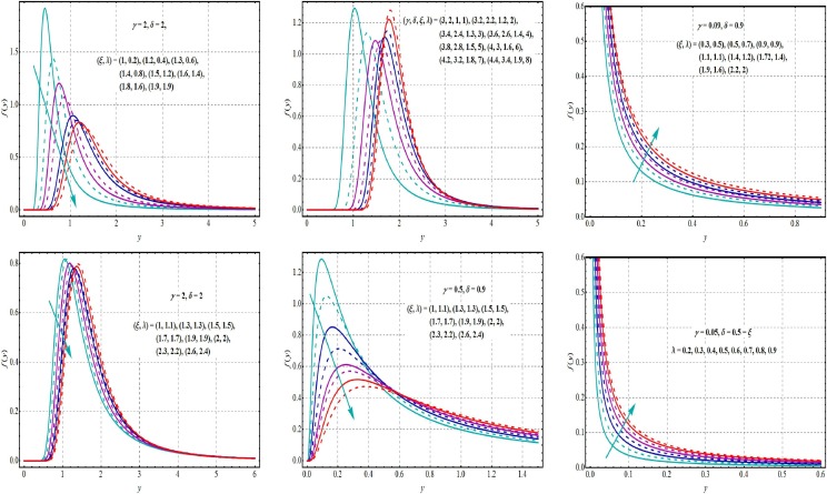
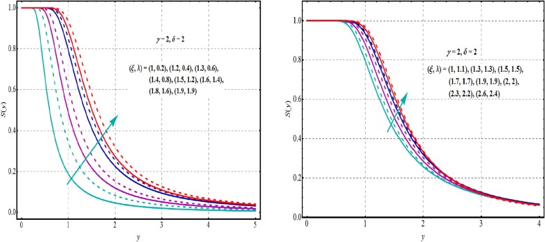
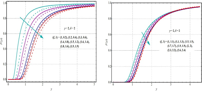
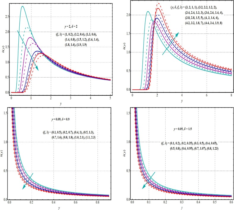
Where $R_y\left(y\right)$and$h_y\left(y\right)$is defined in Eqs. ($7-8)$. Utilizing MATLAB, Mathematica, Maple, R and Minitab computing packages, Eqs. (1), (2), (3), (4), (5), (6), (7), (8), (9), (10) are being evaluated readily. The sketches of Eq. $\left(5\right)$, Eq. $\left(6\right)$ and Eq. $\left(8\right)$are shown in Figs. 1 2 and 3 for different options of the parameters. Fig. 1 shows influence of $\lambda$on density of GLET-GTII and demonstrates flexibility of the pdf in Eq. $\left(5\right)$forms where low symmetry, modality, high tails and skewness can be evaluated directly. Such figures show the flexibility of the GLET-GTII model. Fig. 2, Fig. 3 are plotted for the $S\left(y\right)$and CDF of the GLET-GTII. On the other hand, decreasing and upside bathtub pattern of hrfs are noted in Fig. 4 . It is also observed that for given value of $\gamma ,\delta ,\xi$and $\lambda >0,h\left(.\right)$indicates the uni-modal behavior.

Fig. 1.

Plots of $f\left(y\right)$of GLET-GTII at different parameteric values.

Fig. 2.

Graphs of $S\left(y\right)$ of GLET-GTII at different values of parameters.

Fig. 3.

Plots of CDF of GLET-GTII at different values of parameters.

Fig. 4.

Graphs of hrf of GLET-GTII for different values of parameter.

Expansion for pdf

Using geometric infinite sum of series for $\frac{1}{\left(2-e^{-\xi \left(\exp \left\{-\lambda \delta y^{-\gamma }\right\}\right)}\right)}={\sum }_{q=0}^{\infty }\frac{{\left(-1\right)}^q}{2^{q+1}}{e}^{-\xi q\left(\exp \left\{-\lambda \delta y^{-\gamma }\right\}\right)}$. The pdf responds to the following expansion

$$f\left(\left(y\right|\gamma ,\delta ,\xi ,\lambda \right)={\displaystyle \sum _{q=0}^{\infty }}{\left(-1\right)}^q\frac{\xi \gamma \delta \lambda y^{-\gamma -1}{e}^{-\xi \left(\exp \left\{-\lambda \delta y^{-\gamma }\right\}\right)}\exp \left\{-\delta \lambda y^{-\gamma }\right\}{e}^{-\xi q\left(\exp \left\{-\lambda \delta y^{-\gamma }\right\}\right)}}{2^{q+1}\log \left\{2-e^{-\xi }\right\}},$$ (11)

$$f\left(\left(y\right|\gamma ,\delta ,\xi ,\lambda \right)={\displaystyle \sum _{q=0}^{\infty }}{\left(-1\right)}^q\frac{\xi \gamma \lambda \delta y^{-\gamma -1}{e}^{-\xi \left(q+1\right)\left(\exp \left\{-\lambda \delta y^{-\gamma }\right\}\right)}\exp \left\{-\delta \lambda y^{-\gamma }\right\}}{2^{q+1}\log \left\{2-e^{-\xi }\right\}},$$ (12)

and now using exponential series $e^{-x}={\sum }_{n=0}^{\infty }{\left(-1\right)}^n\frac{x^n}{n!}$ in Eq. (12) we have

$$f\left(\left(y\right|\gamma ,\delta ,\xi ,\lambda \right)={\displaystyle \sum _{k,q,p=0}^{\infty }}{\left(-1\right)}^{k+q+p}\frac{{\xi }^{k+p+1}\lambda \gamma \delta y^{-\gamma -1}{q}^k\exp \left\{-\left(k+p+1\right)\delta \lambda y^{-\gamma }\right\}}{k!p!2^{q+1}\log \left\{2-e^{-\xi }\right\}}\text{.}$$ (13)

Random number generator

Let r.v. $q~U(0,1)$. Then Y is obtained as

$$\log \left\{2-e^{-\xi \left(\exp \left\{-\delta y^{-\gamma }\right\}\right)}\right\}=q\left[\log \left\{2-e^{-\xi }\right\}\right],$$ (14)

$$\log \left\{2-e^{-\xi \left(\exp \left\{-\lambda \delta y^{-\gamma }\right\}\right)}\right\}=\log {\left\{2-e^{-\xi }\right\}}^q,$$

$$e^{-\xi \left(\exp \left\{-\lambda \delta y^{-\gamma }\right\}\right)}=2-{\left\{2-e^{-\xi }\right\}}^q,$$

$$\exp \left\{-\lambda \delta y^{-\gamma }\right\}=-\frac{1}{\xi }\log \left[2-{\left\{2-e^{-\xi }\right\}}^q\right],$$

$$\begin{array}{cc}\hfill Y=& \mathbb{Q}\left(\delta ,\gamma ,\xi ,\lambda \right),\hfill \\ \hfill =& {\left(-\frac{1}{\delta }\log {\left(-\frac{1}{\xi }\log \left[2-{\left\{2-e^{-\xi }\right\}}^q\right]\right)}^{\frac{1}{\lambda }}\right)}^{-\frac{1}{\gamma }}~\mathrm{GLET}-\mathrm{GTII}\left(\gamma ,\delta ,\xi ,\lambda \right)\text{.}\hfill \end{array}$$ (15)

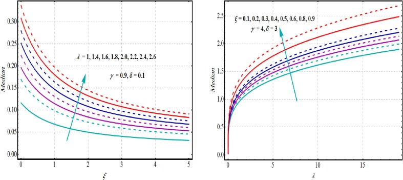
Particularly, by placing $q=0.25,0.50,0.75$ in Eq. (15), $I^{\mathit{st}}$ and $3^{\mathit{rd}}$ quartile and median are attained.

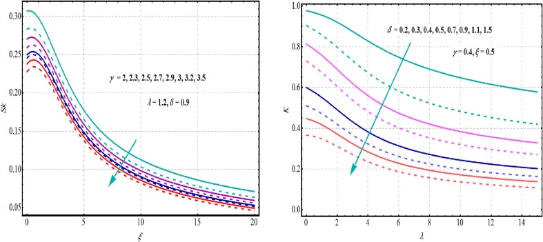
Significant measurements of kurtosis and skewness are ${\varphi }_4={\mu }_4/{\sigma }^4$ and ${\varphi }_3={\mu }_3/{\sigma }^3$, respectively, in which fundamental ${\kappa }^{\mathit{th}}$ moment represents by ${\mu }_{\kappa }$ and standard deviation represents by $\sigma$. As moments of GLET-GTII model can not occur for some values of parameter, suitable indicators for quantile-based ${\mathrm{S}}_{\mathit{kewness}}$ and ${\mathrm{K}}_{\mathit{urtosis}}$ are more appropriate. These indicators are more robust and do exists for distributions in the absence of moments. $S_B$ (Bowley’s Skewness) and $K_M$ (Moors’ Kurtosis) measures are specified as

$$S_B=\frac{F^{-1}\left(6/8\right)+F^{-1}\left(2/8\right)-2F^{-1}\left(\left(4/8\right|\right)}{F^{-1}\left(6/8\right)-F^{-1}\left(2/8\right)},$$ (16)

$$K_M=\frac{F^{-1}\left(7/8\right)-F^{-1}\left(5/8\right)+F^{-1}\left(3/8\right)-F^{-1}\left(1/8\right)}{F^{-1}\left(6/8\right)-F^{-1}\left(2/8\right)}\text{.}$$ (17)

When $S_B<0$ and $S_B>0$, then model is left and right skewed respectively and is symmetrical for $S_B=0$. Instead, a large $K_M$ indicates a heavy tail for the distribution and a mild tail for a low $K_M$ .

Fig. 5 is plotted to analyze the influence of $S_B$ and $K_M$ in light of GLET-GTII model and as per parametric values. In Fig. 6 , the behavior of median in relation of GLET-GTII model is sketched.

Fig. 5.

Plots of skewness and kurtosis of GLET-GTII model.

Fig. 6.

graphs for Median of GLET-GTII model.

Table 1 displays the numerical values of ${\mu }_1^{\prime },{\mu }_2^{\prime },{\mu }_3^{\prime },{\mu }_4^{\prime }$, Variance, $C.V$., ${\left(K_M\right|}_{\gamma ,\delta ,\xi ,\lambda }$ and ${\left(S_B\right|}_{\gamma ,\delta ,\xi ,\lambda }$ for GLET-GTII distribution. From Table 1, the considerable effects of $\gamma ,\delta ,\xi$and $\lambda$are noted on abovementioned measures.

Table 1.

Numerical values of descriptive measures.

$\gamma$	$\delta$	$\xi$	$\lambda$	${\mu }_1^{\prime }$	${\mu }_2^{\prime }$	${\mu }_3^{\prime }$	${\mu }_4^{\prime }$	Var	C.V.	$S_B$	$K_M$
4	0.5	0.2	0.1	0.55998	0.36764	0.33854	31888.2	0.05407	41.5235	0.21837	1.40271
4	0.5	0.3	0.5	0.82490	0.79528	1.07101	146747	0.11481	41.0760	0.21985	1.40681
4	0.5	0.5	1.0	0.95479	1.05892	1.62699	251366	0.14730	40.1976	0.22174	1.41427
4	0.5	0.7	2.0	1.10831	1.41826	2.49258	434625	0.18991	39.3201	0.22231	1.42059
5	0.5	0.2	0.1	0.62253	0.42404	0.334708	0.36499	0.03649	30.6842	0.20018	1.37502
5	1.0	0.3	0.5	0.97511	1.03837	1.27836	2.16801	0.08753	30.3398	0.20201	1.37923
5	1.5	0.5	1.0	1.18923	1.53875	2.29114	4.67117	0.12449	29.6684	0.20456	1.38702
5	2.0	0.7	2.0	1.41984	2.18552	3.85298	9.24075	0.169578	29.0031	0.20575	1.39382
6	3.5	0.2	1.0	1.36045	1.96148	3.07591	5.54933	0.11066	24.4514	0.18799	1.35782
6	3.5	0.3	1.5	1.44154	2.19945	3.64442	6.93488	0.12140	24.17	0.19226	1.36207
6	3.5	0.5	2.0	1.48619	2.33203	3.96212	7.70249	0.12326	23.6234	0.19305	1.37001
6	3.5	0.7	2.5	1.51871	2.42939	4.19528	8.25804	0.12291	23.0847	0.19465	1.37707

Order statistics

Order statistics (OS) exist in several fields of theory and functional statistics. Suppose $Y_{\left(1\right)}⩽Y_{\left(2\right)}⩽\dots ⩽Y_{\left(n\right)}$ is OS of a random sample of n size from $F\left(y\right)$. Then, for $m=1,2,\dots ,n$, probability density function of $m^{\mathit{th}}$ OS, $Y_{\left(m\right)}$ is given by

$$f_{\left(m\right)}\left(\left(y\right|\gamma ,\delta ,\xi ,\lambda \right)=\mathrm{\Psi }F{\left(\left(y\right|\gamma ,\delta ,\xi ,\lambda \right)}^{m-1}{\left\{1-F\left(\left(y\right|\gamma ,\delta ,\xi ,\lambda \right)\right\}}^{n-m}f\left(\left(y\right|\gamma ,\delta ,\xi ,\lambda \right),$$ (18)

where $\mathrm{\Psi }=\frac{n!}{\left(m-1\right)!\left(n-m\right)!}$, where $F(·)$ and $f(·)$ are cdf and pdf of GLET-GTII, accordingly.Utilizing the specification of binomial expansion for term:${\left\{1-F\left(\left(y\right|b,\eta \right)\right\}}^{n-m}$. Thus from Eq. (5), Eq. (6) and Eq. (18), probability density function of $Y_{\left(m\right)}$ as

$$f_{\left(m\right)}\left(\left(y\right|\gamma ,\delta ,\xi ,\lambda \right)=\mathrm{\Psi }{\displaystyle \sum _{f=0}^{n-m}}{\left(-1\right)}^f\left(\begin{array}{c}\hfill n-m\hfill \\ \hfill f\hfill \end{array}\right)F{\left(\left(y\right|\gamma ,\delta ,\xi ,\lambda \right)}^{m+f-1}f\left(\left(y\right|\gamma ,\delta ,\xi ,\lambda \right)\text{.}$$

The cdf of $Y_{\left(m\right)}$ is

$$F_{\left(m\right)}\left(\left(y\right|\gamma ,\delta ,\xi ,\lambda \right)={\displaystyle \sum _{j=m}^n}\left(\begin{array}{c}\hfill n\hfill \\ \hfill j\hfill \end{array}\right)F{\left(\left(y\right|\gamma ,\delta ,\xi ,\lambda \right)}^j{\left\{1-F\left(\left(y\right|\gamma ,\delta ,\xi ,\lambda \right)\right\}}^{n-j}\text{.}$$ (19)

In particular, cummulative density functions of $Y_{\left(1\right)}$ and $Y_{\left(n\right)}$ respectively, are given by

$$F_{\left(n\right)}\left(y\right)={\left(F\left(y\right)\right)}^n,F_{\left(1\right)}\left(y\right)=1-{\left\{1-F\left(y\right)\right\}}^n$$ (20)

Let ${\mathbb{Q}}_{\left(m\right)}^{\ast }\left(.\right)$is quantile function of $Y_{\left(m\right)}$ (for $0<q<1)$. Then, from Eq. $\left(20\right)$

$${\mathbb{Q}}_{\left(1\right)}^{\ast }\left(q\right)={\mathbb{Q}}^{\ast }\left\{1-{\left[1-q\right]}^{1/n}\right\},{\mathbb{Q}}_{\left(n\right)}^{\ast }\left(q\right)={\mathbb{Q}}^{\ast }\left(q^{1/n}\right),$$

where quantile function of Y is ${\mathbb{Q}}^{\ast }\left(.\right)$. For i.i.d. random values case, it is feasible to obtain $s^{\mathit{th}}$ ordinary moment expression of the order statistics for ${\acute{\mu }}_s<\infty$. So, as Silva et al. [16], the ${\acute{\mu }}_s$ moment of $m^{\mathit{th}}$ order statistic $Y_{\left(m\right)}$ as

(21)

where ${}_j\left(s\right)=s{\int }_0^{\infty }{y}^{s-1}{\left\{1-F\left(y\right)\right\}}^j\mathit{dy}$. In particular, for the GLET-GTII distribution, we obtain

$${\acute{\mu }}_{\left(m\right)}^s=s{\displaystyle \sum _{j=n-m+1}^n}\left(\begin{array}{c}\hfill j-1\hfill \\ \hfill n-m\hfill \end{array}\right)\left(\begin{array}{c}\hfill n\hfill \\ \hfill j\hfill \end{array}\right){\left(-1\right)}^{j-n+m-1}{\int }_0^{\infty }{y}^{s-1}{\left[1-\frac{\log \left\{2-e^{-\xi \left(\exp \left\{-\lambda \delta y^{-\gamma }\right\}\right)}\right\}}{\log \left\{2-e^{-\xi }\right\}}\right]}^j\mathit{dy}\text{.}$$ (22)

Stochastic ordering (SO)

The notion of SO for continuous positive random variables is a common and effective concept for calculating relative behavior. We must recall some basic meanings. Suppose that r.v. Y is greater than X

(i) Stochastic order (S-O) $Y{⩾}_{\mathit{st}}X$. if $F_Y\left(y\right)⪰F_X\left(y\right)$ $\forall$ y; (ii) hazard rate order (Hr-O) $Y{⩾}_{\mathit{hr}}X$ if $h_X\left(y\right)\succcurlyeq h_Y\left(y\right)$ $\forall$ y; (iii) likelihood ratio order (LHr-O) $Y{⪰}_{\mathit{lr}}X$, if $\frac{f_X\left(y\right)}{f_Y\left(y\right)}$ reduces in y. The below mentioned results are known (see [17]):

$$Y{⪰}_{\mathit{lr}}X\Rightarrow Y{⪰}_{\mathit{hr}}X\Rightarrow Y{⪰}_{\mathit{st}}X\text{.}$$ (23)

The GLET-GTII distributions are ordered with respect to the strongest “likelihood ratio” ordering as mentioned in the following theorem.

Theorem 1

Let $X~$GLET-GTII $\left(\gamma ,\delta ,\xi ,{\lambda }_1\right)$, and $Y~$GLET-GTII $\left(\gamma ,\delta ,\xi ,{\lambda }_2\right)$. If ${\lambda }_1⩽{\lambda }_2$, then $Y{⩾}_{\mathit{lr}}X$ $\left(Y{⩾}_{\mathit{hr}}X,Y{⩾}_{\mathit{st}}X\right)$.

Proof

Consider likelihood ratio (LHr) as

$$\frac{f_X\left(y\right)}{f_Y\left(y\right)}=\frac{{\lambda }_1{\left(e^{-\delta y^{-\gamma }}\right)}^{{\lambda }_1-{\lambda }_2}\left(2e^{e^{-{\lambda }_2\delta y^{-\gamma }}\xi }-1\right)}{{\lambda }_2\left(2e^{e^{-{\lambda }_1\delta y^{-\gamma }}\xi }-1\right)},y>0,$$ (24)

now differentiate Eq. (24) w.r.t y, we attain the expression given below

$$\begin{array}{cc}\hfill \frac{d}{\mathit{dy}}\left(\frac{f_X\left(y\right)}{f_Y\left(y\right)}\right)=& \frac{y^{-\gamma -1}\gamma \delta {\lambda }_1{\left(e^{-\delta y^{-\gamma }}\right)}^{{\lambda }_1-{\lambda }_2}}{{\lambda }_2{\left(1-2e^{e^{-{\lambda }_1\delta y^{-\gamma }}\xi }\right)}^2}\hfill \\ \hfill & \left[-{\lambda }_1\left(2e^{e^{-{\lambda }_2\delta y^{-\gamma }}\xi }-1\right)\left\{1+2e^{e^{-{\lambda }_1\delta y^{-\gamma }}\xi }\left(-1+e^{e^{-{\lambda }_1\delta y^{-\gamma }}\xi }\right)\right\}\right)\hfill \\ \hfill & \left(+{\lambda }_2\left(2e^{e^{-{\lambda }_1\delta y^{-\gamma }}\xi }-1\right)\left\{1+2e^{e^{-{\lambda }_2\delta y^{-\gamma }}\xi }\left(-1+e^{e^{-{\lambda }_2\delta y^{-\gamma }}\xi }\right)\right\}\right],\hfill \end{array}$$ (25)

$$\frac{d}{\mathit{dy}}\left[\frac{f_X\left(y\right)}{f_Y\left(y\right)}\right]⩽0\text{.}$$

Hence it demonstrates that $Y{⩾}_{\mathit{lr}}X$, and according to Eq. (23), $Y{⩾}_{\mathit{hr}}X$, and$Y{⩾}_{\mathit{st}}X$ are also hold.

Moments, central moments and certain related measures

For any statistical consideration, moments are profoundly significant, usually in applications. The special parameters that can be used to describe a homogeneous data set’s behaviour are called moments. Consequently, for GLET-GTII model, the ${\acute{\mu }}_s$ which is $s^{\mathit{th}}$ non-central moment is obtain as follows. If Y has probability density function in Eq. (5), we get

$${\acute{\mu }}_s=E\left(Y^s\right)={\displaystyle \underset{0}{\overset{\infty }{\int }}}{y}^s\mathit{dF}\left(\left(y\right|\gamma ,\delta ,\xi ,\lambda \right)\text{;}s=1,2,\dots$$ (26)

The belowmentioned outcome gives ${\acute{\mu }}_s$ ($s^{\mathit{th}}$ non-central moment) of Y in G-F (gamma function) form.

Theorem 2

For $\gamma ,\delta ,\xi ,\lambda >0$, the ${\acute{\mu }}_s\left(\left(y\right|\gamma ,\delta ,\xi ,\lambda \right)$  of Y is translated as

$${\acute{\mu }}_s\left(\left(y\right|\gamma ,\delta ,\xi ,\lambda \right)={\displaystyle \sum _{p,q,k=0}^{\infty }}{\left(-1\right)}^{p+q+k}\frac{{\xi }^{p+k+1}{\lambda }^{s/\gamma }\delta q^k}{p!k!2^{q+1}\log (2-e^{-\xi }){\left[\delta \left\{p+k+1\right\}\right]}^{1-\frac{s}{\gamma }}}\mathrm{\Gamma }\left(1-s/\gamma \right),$$ (27)

where, usual G-F is $\mathrm{\Gamma }\left(.\right)$.

Proof

Consider

$${\acute{\mu }}_s={\displaystyle \underset{0}{\overset{\infty }{\int }}}{y}^s\mathit{dF}\left(\left(y\right|\gamma ,\delta ,\xi ,\lambda \right)\text{.}$$

By using the expansion form of pdf that given in Eq. (13) yields

$$\begin{array}{cc}\hfill {\acute{\mu }}_s\left(\left(y\right|\gamma ,\delta ,\xi ,\lambda \right)=& {\sum }_{p,q,k=0}^{\infty }{\left(-1\right)}^{p+q+k}\frac{{\xi }^{p+k+1}\lambda \gamma \delta q^k}{p!k!2^{q+1}\log \left\{2-e^{-\xi }\right\}}\hfill \\ \hfill & {\displaystyle \underset{0}{\overset{\infty }{\int }}}{y}^{s-\gamma -1}\exp \left\{-\left(p+k+1\right)\delta \lambda y^{-\gamma }\right\}\mathit{dy}\text{.}\hfill \end{array}$$ (28)

Allowing $z=\left(p+k+1\right)\lambda y^{-\gamma }$ using the result $-\gamma \left(p+k+1\right)\lambda y^{-\gamma -1}\mathit{dy}=\mathit{dz}$ and after some algebraic manipulation we have

$$\begin{array}{cc}\hfill {\acute{\mu }}_s\left(\left(y\right|\gamma ,\delta ,\xi ,\lambda \right)=& {\sum }_{p,q,k=0}^{\infty }{\left(-1\right)}^{p+q+k}\frac{{\xi }^{p+k+1}\lambda \gamma \delta q^k}{p!k!2^{q+1}\log \left\{2-e^{-\xi }\right\}}\hfill \\ \hfill & {\displaystyle \underset{0}{\overset{\infty }{\int }}}{\left(\frac{z}{\left(p+k+1\right)\lambda }\right)}^{\frac{-s}{\gamma }}\frac{\exp (-\delta z)}{\left(p+k+1\right)}\mathit{dz}\text{.}\hfill \end{array}$$ (29)

Since, $\mathrm{\Gamma }\left(\tau \right)$ $=\underset{0}{\overset{\infty }{\int }}{y}^{\tau -1}{e}^{-y}\mathit{dy}$, therefore the above integral provides the sth moment given by Eq. (27).

In particular, the first four moments of Y are:

$${\acute{\mu }}_1={\displaystyle \sum _{p,q,k=0}^{\infty }}{\left(-1\right)}^{p+q+k}\frac{{\xi }^{p+k+1}{\lambda }^{1/r}\delta q^k}{p!k!2^{q+1}\log (2-e^{-\xi }){\left[\delta \left\{p+k+1\right\}\right]}^{1-\frac{1}{\gamma }}}\mathrm{\Gamma }\left(1-1/\gamma \right),$$ (30)

$${\acute{\mu }}_2={\displaystyle \sum _{p,q,k=0}^{\infty }}{\left(-1\right)}^{p+q+k}\frac{{\xi }^{p+k+1}{\lambda }^{2/r}\delta q^k}{p!k!2^{q+1}\log (2-e^{-\xi }){\left[\delta \left\{p+k+1\right\}\right]}^{1-\frac{2}{\gamma }}}\mathrm{\Gamma }\left(1-2/\gamma \right),$$ (31)

$${\acute{\mu }}_3={\displaystyle \sum _{p,q,k=0}^{\infty }}{\left(-1\right)}^{p+q+k}\frac{{\xi }^{p+k+1}{\lambda }^{3/r}\delta q^k}{p!k!2^{q+1}\log (2-e^{-\xi }){\left[\delta \left\{p+k+1\right\}\right]}^{1-\frac{3}{\gamma }}}\mathrm{\Gamma }\left(1-3/\gamma \right),$$ (32)

and

$${\acute{\mu }}_4={\displaystyle \sum _{p,q,k=0}^{\infty }}{\left(-1\right)}^{p+q+k}\frac{{\xi }^{p+k+1}{\lambda }^{4/r}\delta q^k}{p!k!2^{q+1}\log (2-e^{-\xi }){\left[\delta \left\{p+k+1\right\}\right]}^{1-\frac{4}{\gamma }}}\mathrm{\Gamma }\left(1-4/\gamma \right)\text{.}$$ (33)

Proposition 1

Let Y be a random variable following the GLET-GTII distribution, then the central moments is

$$\begin{array}{cc}\hfill {\mu }_s\left(\left(y\right|\gamma ,\delta ,\xi ,\lambda \right)=& \left({\displaystyle \sum _{t=0}^s}{\displaystyle \sum _{p,q,k=0}^{\infty }}\left(\begin{array}{c}\hfill s\hfill \\ \hfill t\hfill \end{array}\right){\left(-1\right)}^{p+q+k+t}\frac{{\mu }^t{\xi }^{p+k+1}{\lambda }^{s-t/r}\delta q^k}{p!k!2^{q+1}\log (2-e^{-\xi }){\left[\delta \left\{p+k+1\right\}\right]}^{1-\frac{s-t}{\gamma }}}\right)\hfill \\ \hfill & \times \left(\mathrm{\Gamma }\left(1-\left(s-t\right)/\gamma \right)\right),\hfill \end{array}$$ (34)

where, $\mathrm{\Gamma }\left(.\right)$ is usual gamma function.

$${\mu }_s\left(\left(y\right|\gamma ,\delta ,\xi ,\lambda \right)={\displaystyle \underset{0}{\overset{\infty }{\int }}}{\left(y-\mu \right)}^{s}f\left(y\right)\mathit{dy}$$ (35)

Substituting by the Eq. (27) into Eq. (35) after certain simple calculations, we get

$$\begin{array}{cc}\hfill {\mu }_s\left(\left(y\right|\gamma ,\delta ,\xi ,\lambda \right)=& \left({\displaystyle \sum _{t=0}^s}{\displaystyle \sum _{p,q,k=0}^{\infty }}\left(\begin{array}{c}\hfill s\hfill \\ \hfill t\hfill \end{array}\right){\left(-1\right)}^{p+q+k+t}\frac{{\mu }^t{\xi }^{p+k+1}{\lambda }^{s-t/r}\delta q^k}{p!k!2^{q+1}\log (2-e^{-\xi }){\left[\delta \left\{p+k+1\right\}\right]}^{1-\frac{s-t}{\gamma }}}\right)\hfill \\ \hfill & \left(\mathrm{\Gamma }\left(1-\left(s-t\right)/\gamma \right)\right)\text{.}\hfill \end{array}$$ (36)

Remark 1

The variance of GLET-GTII model is obtained from Equation (36) for $s=2$.

Moment generating function (mgf)

The mgf of GLET-GTII distribution may be indicated as

$$\begin{array}{cc}\hfill M\left(\left(y\right|\gamma ,\delta ,\xi ,\lambda \right)=& {\sum }_{s=0}^{\infty }\frac{t^s}{s!}{\acute{\mu }}_s\left(\left(y\right|\gamma ,\delta ,\xi ,\lambda \right),\hfill \\ \hfill =& \left({\displaystyle \sum _{s,p,q,k=0}^{\infty }}\frac{t^s}{s!}{\left(-1\right)}^{p+q+k}\frac{{\xi }^{p+k+1}{\lambda }^{s/r}\delta q^k}{p!k!2^{q+1}\log (2-e^{-\xi }){\left[\delta \left\{p+k+1\right\}\right]}^{1-\frac{s}{\gamma }}}\right)\hfill \\ \hfill & \times \left(\mathrm{\Gamma }\left(1-s/\gamma \right)\right)\text{.}\hfill \end{array}$$ (37)

Characteristic function (cf)

For GLET-GTII model, cf is evaluated as

$$\mathrm{\Phi }\left(\left(\tau y\right|\gamma ,\delta ,\xi ,\lambda \right)={\displaystyle \underset{0}{\overset{\infty }{\int }}}{e}^{i\tau y}\mathit{dF}\left(\left(y\right|\gamma ,\delta ,\xi ,\lambda \right)\text{.}$$ (38)

After using exponential series, we have

$$\mathrm{\Phi }\left(\left(\tau y\right|\gamma ,\delta ,\xi ,\lambda \right)={\displaystyle \sum _{s=0}^{\infty }}\frac{{\left(i\tau \right)}^s}{s!}{\displaystyle \underset{0}{\overset{\infty }{\int }}}{y}^s\mathit{dF}\left(\left(y\right|\gamma ,\delta ,\xi ,\lambda \right)\text{.}$$ (39)

Hence, we obtain

$$\mathrm{\Phi }\left(\left(\tau y\right|\gamma ,\delta ,\xi ,\lambda \right)={\displaystyle \sum _{s,p,q,k=0}^{\infty }}\frac{{\left(i\tau \right)}^s}{s!}{\left(-1\right)}^{p+q+k}\frac{{\xi }^{p+k+1}{\lambda }^{s/r}\delta q^k\mathrm{\Gamma }\left(1-s/\gamma \right)}{p!k!2^{q+1}\log (2-e^{-\xi }){\left[\delta \left\{p+k+1\right\}\right]}^{1-\frac{s}{\gamma }}}\text{.}$$ (40)

Factorial generating function (fgf)

For GLET-GTII model, fgf is extracted as follows

$$\begin{array}{cc}\hfill F_y\left(\left(\tau y\right|\gamma ,\delta ,\xi ,\lambda \right)=& {\displaystyle \underset{0}{\overset{\infty }{\int }}}{e}^{\log {\left(1+\tau \right)}^y}\mathit{dF}\left(\left(y\right|\gamma ,\delta ,\xi ,\lambda \right),\hfill \\ \hfill =& {\sum }_{s=0}^{\infty }\frac{{\left(\log \left(1+\tau \right)\right)}^s}{s!}{\displaystyle \underset{0}{\overset{\infty }{\int }}}{y}^s\mathit{dF}\left(\left(y\right|\gamma ,\delta ,\xi ,\lambda \right),\hfill \end{array}$$ (41)

so,

$$\begin{array}{cc}\hfill F_y\left(\left(\tau y\right|\gamma ,\delta ,\xi ,\lambda \right)=& \left({\displaystyle \sum _{s,p,q,k=0}^{\infty }}\frac{{\left(\log \left(1+\tau \right)\right)}^s}{s!}{\left(-1\right)}^{p+q+k}\right)\hfill \\ \hfill & \times \left(\frac{{\xi }^{p+k+1}{\lambda }^{s/r}\delta q^k}{p!k!2^{q+1}\log (2-e^{-\xi }){\left[\delta \left\{p+k+1\right\}\right]}^{1-\frac{s}{\gamma }}}\mathrm{\Gamma }\left(1-s/\gamma \right)\right)\text{.}\hfill \end{array}$$ (42)

Incomplete non-central moments (INCM)

The INCM of model serve as a key role in determining inequality, namely Lorenz and Bonferroni’s income quantiles and curves, which concentrate on incomplete moments.

Proposition 2

The $s^{\mathit{th}}$ incomplete moment ${\acute{\mu }}_{Y,s}\left(z,\gamma ,\delta ,\xi ,\lambda \right)$is

$$\begin{array}{cc}\hfill {\acute{\mu }}_{Y,s}\left(z,\gamma ,\delta ,\xi ,\lambda \right)=& \left({\displaystyle \sum _{p,q,k=0}^{\infty }}{\left(-1\right)}^{p+q+k}\frac{{\xi }^{p+k+1}{\lambda }^{s/r}\delta q^k}{p!k!2^{q+1}\log (2-e^{-\xi }){\left[\delta \left\{p+k+1\right\}\right]}^{1-\frac{s}{\gamma }}}\right)\hfill \\ \hfill & \times \left(\mathrm{\Gamma }\left\{1-\frac{s}{\gamma },z^{-\gamma }\delta \lambda \left(p+k+1\right)\right\}\right),\hfill \end{array}$$ (43)

where, $\mathrm{\Gamma }\left(a,x\right)={\int }_x^{\infty }{t}^{a-1}{e}^{-t}\mathit{dt}$ is upper incomplete G-F.

Proof

By definition

$${\acute{\mu }}_{Y,s}\left(z,\gamma ,\delta ,\xi ,\lambda \right)={\displaystyle \underset{0}{\overset{z}{\int }}}{y}^s\mathit{dF}\left(\left(y\right|\gamma ,\delta ,\xi ,\lambda \right),s=1,2,\dots$$ (44)

Substituting by the Eq. (13) into Eq. (44) after some simple calculations, we have

$${\acute{\mu }}_{Y,s}\left(z,\gamma ,\delta ,\xi ,\lambda \right)={\displaystyle \sum _{p,q,k=0}^{\infty }}{\left(-1\right)}^{p+q+k}\frac{{\xi }^{p+k+1}\lambda \gamma \delta q^k}{p!k!2^{q+1}\log \left\{2-e^{-\xi }\right\}}{\displaystyle \underset{0}{\overset{z}{\int }}}{y}^{s-\gamma -1}\exp \left\{-\left(k+p+1\right)\delta \lambda y^{-\gamma }\right\}\mathit{dy}\text{.}$$

Allowing $w=\left(p+k+1\right)\lambda y^{-\gamma }$ using the result $-\gamma \left(p+k+1\right)\lambda y^{-\gamma -1}\mathit{dy}=\mathit{dw}$ and after some algebraic manipulation we have

$$\begin{array}{cc}\hfill {\acute{\mu }}_{Y,s}\left(z,\gamma ,\delta ,\xi ,\lambda \right)=& \left({\displaystyle \sum _{p,q,k=0}^{\infty }}{\left(-1\right)}^{p+q+k}\frac{{\xi }^{p+k+1}\lambda \gamma \delta q^k}{p!k!2^{q+1}\log \left\{2-e^{-\xi }\right\}}\right)\hfill \\ \hfill & \times \left({\displaystyle \underset{\left(p+k+1\right)\lambda z^{-\gamma }}{\overset{\infty }{\int }}}{\left(\frac{z}{\left(p+k+1\right)\lambda }\right)}^{\frac{-s}{\gamma }}\frac{\exp (-\delta w)}{\left(p+k+1\right)}\mathit{dw}\right)\text{.}\hfill \end{array}$$ (45)

The above integral provides the sth moment given by Eq. (45).

Lemma 1

$\bar{I}\left(a,\gamma ,\delta ,\xi ,\lambda \right)=\underset{a}{\overset{\infty }{\int }}\mathit{ydF}\left(\left(y\right|\gamma ,\delta ,\xi ,\lambda \right)$ we have

$$\begin{array}{cc}\hfill \bar{I}\left(a,\gamma ,\delta ,\xi ,\lambda \right)=& \left({\displaystyle \sum _{p,q,k=0}^{\infty }}{\left(-1\right)}^{p+q+k}\frac{{\xi }^{p+k+1}{\lambda }^{1/r}\delta q^k}{p!k!2^{q+1}\log (2-e^{-\xi }){\left[\delta \left\{p+k+1\right\}\right]}^{1-\frac{1}{\gamma }}}\right)\hfill \\ \hfill & \left(\mathrm{\Gamma }\left\{a^{-\gamma }\delta \lambda \left(p+k+1\right),1-\frac{1}{\gamma }\right\}\right),\hfill \end{array}$$ (46)

where $\mathrm{\Gamma }\left(x,a\right)={\int }_0^x{t}^{a-1}{e}^{-t}\mathit{dt}$ is lower incomplete gamma function.

Conditional moments and mean deviations

In predictive inference, the estimation of conditional moments ${\left(E\left(\left(Y^s\right|Y>t\right)\right|}_{s=1,2,\dots }$ is useful in interaction with lifetime models. The $E\left(\left(Y^s\right|Y>t\right)$is obtained as

$$\begin{array}{cc}\hfill E\left(\left(Y^s\right|Y>t\right)=& \frac{1}{S\left(t\right)}\left[E\left(Y^s\right)-{\displaystyle \underset{0}{\overset{t}{\int }}}{y}^{s}f\left(y\right)\mathit{dy}\right],\hfill \\ \hfill =& \frac{1}{S\left(t\right)}\left[\left({\acute{\mu }}_s\left(\left(y\right|\gamma ,\delta ,\xi ,\lambda \right)-{\acute{\mu }}_{Y,s}\left(t,\gamma ,\delta ,\xi ,\lambda \right)\right)\right],\hfill \end{array}$$ (47)

where $S\left(t\right),{\acute{\mu }}_s$, and ${\acute{\mu }}_{Y,s}$ are defined in Eqs. (7), (27), (43). The mean deviations about mean $\mu =E\left(Y\right)$ and $\tilde{\mu }$ (median) are stated as

$${\mathrm{\Theta }}_1\left(Y\right)={\int }_0^{\infty }\left|y-\mu \right|\mathit{dF}\left(\left(y\right|\gamma ,\delta ,\xi ,\lambda \right),$$ (48)

and

$${\mathrm{\Theta }}_2\left(Y\right)={\int }_0^{\infty }\left|y-\tilde{\mu }\right|\mathit{dF}\left(\left(y\right|\gamma ,\delta ,\xi ,\lambda \right),$$ (49)

respectively. The quantity ${\mathrm{\Theta }}_1\left(Y\right)$ and ${\mathrm{\Theta }}_2\left(Y\right)$are calculated as follows,

$${\mathrm{\Theta }}_1\left(Y\right)=2{\int }_{\mu }^{\infty }\mathit{yf}\left(y\right)\mathit{dy}-2\mu +2\mu F\left(\mu \right),$$ (50)

$${\mathrm{\Theta }}_2\left(Y\right)=2{\int }_{\tilde{\mu }}^{\infty }\mathit{yF}\left(y\right)\mathit{dy}-\mu ,$$ (51)

using Lemma 1, we have

$${\mathrm{\Theta }}_1\left(Y\right)=2\bar{I}\left(\mu ,\gamma ,\delta ,\xi ,\lambda \right)+2\mu F\left(\mu \right)-2\mu ,$$ (52)

$${\mathrm{\Theta }}_2\left(Y\right)=2\bar{I}\left(\tilde{\mu },\gamma ,\delta ,\xi ,\lambda \right)-\mu ,$$ (53)

where $F\left(\mu \right)$is specified in $\left(6\right)$.

Uncertainty measures

In this section, entropies such as Verma, Renyi entropy, Tsallis etc for GLET-GTII model are being investigated.

Entropy measures

Entropy is a significant idea in several relevant fields communications, measure-preserving dynamical systems, information theory, topological dynamics, thermodynamics, statistical mechanics etc, as a calculation of different characteristics such as uncertainty, disorder, randomness, energy that cannot produce work, complexity, etc. There are many definitions of entropy and they are not inherently ideal for all applications.

Renyi entropy ${\tilde{\mathrm{R}}}_{\sigma }\left(Y\right)$

For GLET-GTII model, the ${\tilde{\mathrm{R}}}_{\sigma }\left(Y\right)$is

$${\tilde{\mathrm{R}}}_{\sigma }\left(Y\right)=\frac{1}{1-\sigma }\log {\displaystyle \underset{0}{\overset{\infty }{\int }}}{f}^{\sigma }\left(\left(y\right|\gamma ,\delta ,\xi ,\lambda \right)\mathit{dy},\sigma \ne 1,\sigma >0,$$ (54)

where

$$\begin{array}{cc}\hfill f^{\sigma }\left(\left(y\right|\gamma ,\delta ,\xi ,\lambda \right)=& {\left(\frac{\xi \lambda \gamma \delta y^{-\gamma -1}{e}^{-\xi \left(\exp \left\{-\lambda \delta y^{-\gamma }\right\}\right)}\exp \left\{-\delta \lambda y^{-\gamma }\right\}}{\log \left\{2-e^{-\xi }\right\}\left(2-e^{-\xi \left(\exp \left\{-\lambda \delta y^{-\gamma }\right\}\right)}\right)}\right)}^{\sigma },\hfill \\ \hfill =& \left({\displaystyle \sum _{p,q,k=0}^{\infty }}{\left(-1\right)}^{p+k}\frac{{\xi }^{p+k+\sigma }{\left(\lambda \gamma \delta \right)}^{\sigma }{\sigma }^p{q}^k{y}^{-\sigma \left(\gamma +1\right)}}{p!k!q!2^{q+\sigma }}\right)\hfill \\ \hfill & \times \left(\frac{\exp \left\{-\left(p+k+\sigma \right)\delta \lambda y^{-\gamma }\right\}\mathrm{\Gamma }\left(\sigma +q\right)}{\mathrm{\Gamma }\left(\sigma \right){\left(\log \left\{2-e^{-\xi }\right\}\right)}^{\sigma }}\right)\text{.}\hfill \end{array}$$ (55)

By using the above information, we have

$$\begin{array}{cc}\hfill {\displaystyle \underset{0}{\overset{\infty }{\int }}}{f}^{\sigma }\left(\left(y\right|\gamma ,\delta ,\xi ,\lambda \right)\mathit{dy}=& \left({\displaystyle \sum _{p,q,k=0}^{\infty }}{\left(-1\right)}^{p+k}\frac{\mathrm{\Gamma }\left(\sigma +q\right){\xi }^{p+k+\sigma }{\left(\lambda \gamma \delta \right)}^{\sigma }{\sigma }^p{q}^k}{p!k!q!2^{q+\sigma }\mathrm{\Gamma }\left(\sigma \right){\left(\log \left\{2-e^{-\xi }\right\}\right)}^{\sigma }}\right)\hfill \\ \hfill & \times \left({\displaystyle \underset{0}{\overset{\infty }{\int }}}{y}^{-\sigma \left(\gamma +1\right)}\exp \left\{-\left(p+k+\sigma \right)\delta \lambda y^{-\gamma }\right\}\mathit{dy}.\right)\hfill \end{array}$$ (56)

Now substituting, $\left(p+k+\sigma \right)\lambda y^{-\gamma }=z$, the above integral becomes

$$\begin{array}{cc}\hfill {\displaystyle \underset{0}{\overset{\infty }{\int }}}{f}^{\sigma }\left(\left(y\right|\gamma ,\delta ,\xi ,\lambda \right)\mathit{dy}=& \left({\displaystyle \sum _{p,q,k=0}^{\infty }}{\left(-1\right)}^{p+k}\frac{\mathrm{\Gamma }\left(\sigma +q\right){\xi }^{p+k+\sigma }{\left(\lambda \gamma \delta \right)}^{\sigma }{\sigma }^p{q}^k}{\mathrm{\Gamma }\left(\sigma \right)p!k!q!2^{q+\sigma }{\left(\log \left\{2-e^{-\xi }\right\}\right)}^{\sigma }}\right)\hfill \\ \hfill & \times \left({\displaystyle \underset{0}{\overset{\infty }{\int }}}{z}^{-\left(1-\sigma \right)\left(\frac{\gamma +1}{\gamma }\right)}{e}^{-\delta z}\mathit{dz}.\right)\hfill \end{array}$$ (57)

After simplification, we have

$$\begin{array}{cc}\hfill {\displaystyle \underset{0}{\overset{\infty }{\int }}}{f}^{\sigma }\left(\left(y\right|\gamma ,\delta ,\xi ,\lambda \right)\mathit{dy}=& \left({\displaystyle \sum _{p,q,k=0}^{\infty }}{\left(-1\right)}^{p+k}\frac{\mathrm{\Gamma }\left(\sigma +q\right){\xi }^{p+k+\sigma }{\lambda }^{(1-\sigma )/\gamma }{\gamma }^{\sigma -1}{\delta }^{\sigma }{\sigma }^p{q}^k}{\mathrm{\Gamma }\left(\sigma \right)p!k!q!2^{q+\sigma }{\left(\log \left\{2-e^{-\xi }\right\}\right)}^{\sigma }}\right)\hfill \\ \hfill & \times \left(\frac{\mathrm{\Gamma }\left\{1-\left(\frac{\gamma +1}{\gamma }\right)\left(1-\sigma \right)\right\}}{{\delta }^{1-\left(\frac{\gamma +1}{\gamma }\right)\left(1-\sigma \right)}}\right)\text{.}\hfill \end{array}$$ (58)

Finally, ${\tilde{\mathrm{R}}}_{\sigma }\left(Y\right)$becomes

$$\begin{array}{cc}\hfill {\tilde{\mathrm{R}}}_{\sigma }\left(Y\right)=& \frac{1}{1-\sigma }\log \left\{{\displaystyle \sum _{p,q,k=0}^{\infty }}{\left(-1\right)}^{p+k}\frac{\mathrm{\Gamma }\left(\sigma +q\right){\xi }^{p+k+\sigma }{\lambda }^{(1-\sigma )/\gamma }{\gamma }^{\sigma -1}{\delta }^{\sigma }{\sigma }^p{q}^k}{\mathrm{\Gamma }\left(\sigma \right)p!k!q!2^{q+\sigma }{\left(\log \left\{2-e^{-\xi }\right\}\right)}^{\sigma }}\right)\hfill \\ \hfill & \times \left(\frac{\mathrm{\Gamma }\left\{1-\left(\frac{\gamma +1}{\gamma }\right)\left(1-\sigma \right)\right\}}{{\delta }^{1-\left(\frac{\gamma +1}{\gamma }\right)\left(1-\sigma \right)}}\right\}\text{.}\hfill \end{array}$$ (59)

It should be remembered that Shannon entropy of a $r.v$. Y is attained as a special case of ${\tilde{\mathrm{R}}}_{\sigma }\left(Y\right)$when $\sigma \to 1$.

Verma Entropy $V_{\alpha ,\beta }\left(Y\right)$

For GLET-GTII model, the $V_{\alpha ,\beta }\left(Y\right)$is

$$V_{\alpha ,\beta }\left(Y\right)=\frac{1}{\alpha -\beta }\log {\displaystyle \underset{-\infty }{\overset{\infty }{\int }}}{f}^{\alpha +\beta -1}\left(\left(y\right|\gamma ,\delta ,\xi ,\lambda \right)\mathit{dy},\alpha -1<\beta <\alpha ,\alpha ⩾1,\alpha \ne \beta ,$$ (60)

where

$$\begin{array}{cc}\hfill f^{\alpha +\beta -1}\left(\left(y\right|\gamma ,\delta ,\xi ,\lambda \right)=& {\left(\frac{\xi \lambda \gamma \delta y^{-\gamma -1}{e}^{-\xi \left(\exp \left\{-\lambda \delta y^{-\gamma }\right\}\right)}\exp \left\{-\delta \lambda y^{-\gamma }\right\}}{\log \left\{2-e^{-\xi }\right\}\left(2-e^{-\xi \left(\exp \left\{-\lambda \delta y^{-\gamma }\right\}\right)}\right)}\right)}^{\alpha +\beta -1},\hfill \\ \hfill =& \left({\displaystyle \sum _{p,q,k=0}^{\infty }}{\left(-1\right)}^{p+k}\frac{{\xi }^{p+k+\alpha +\beta -1}{\left(\lambda \gamma \delta \right)}^{\alpha +\beta -1}{\left(\alpha +\beta -1\right)}^p{q}^k{y}^{-\left(\alpha +\beta -1\right)\left(\gamma +1\right)}}{p!k!q!2^{q+\sigma }}\right)\hfill \\ \hfill & \times \left(\frac{\exp \left\{-\left(p+k+\alpha +\beta -1\right)\delta \lambda y^{-\gamma }\right\}\mathrm{\Gamma }\left(\alpha +\beta -1+q\right)}{\mathrm{\Gamma }\left(\alpha +\beta -1\right){\left(\log \left\{2-e^{-\xi }\right\}\right)}^{\alpha +\beta -1}}\right)\text{.}\hfill \end{array}$$ (61)

It is significant to remember that, when $\alpha \to 1$, in (60), it reduces to ${\tilde{\mathrm{R}}}_{\sigma }\left(Y\right)$. On the other hand, if $\beta \to 1$ and $\alpha \to 1$, in (60), then it approaches to the Shannon entropy. By using abovementioned information, we get

$$\begin{array}{cc}\hfill {\displaystyle \underset{0}{\overset{\infty }{\int }}}{f}^{\alpha +\beta -1}\left(\left(y\right|\gamma ,\delta ,\xi ,\lambda \right)\mathit{dy}=& \left({\displaystyle \sum _{p,q,k=0}^{\infty }}{\left(-1\right)}^{p+k}\frac{{\xi }^{p+k+\alpha +\beta -1}{\left(\lambda \gamma \delta \right)}^{\alpha +\beta -1}{\left(\alpha +\beta -1\right)}^p{q}^k}{p!k!q!2^{q+\alpha +\beta -1}}\right)\hfill \\ \hfill & \times \frac{\mathrm{\Gamma }\left(\alpha +\beta -1+q\right)}{\mathrm{\Gamma }\left(\alpha +\beta -1\right){\left(\log \left\{2-e^{-\xi }\right\}\right)}^{\alpha +\beta -1}}\hfill \\ \hfill & \left({\displaystyle \underset{0}{\overset{\infty }{\int }}}{y}^{-\left(\alpha +\beta -1\right)\left(\gamma +1\right)}{e}^{-\left(p+k+\alpha +\beta -1\right)\delta \lambda y^{-\gamma }}\mathit{dy}\right)\text{.}\hfill \end{array}$$ (62)

Now substituting, $\lambda \left(p+k+\alpha +\beta -1\right)y^{-\gamma }=t$,the above integral becomes

$$\begin{array}{cc}\hfill {\displaystyle \underset{0}{\overset{\infty }{\int }}}{f}^{\alpha +\beta -1}\left(\left(y\right|\gamma ,\delta ,\xi ,\lambda \right)\mathit{dy}=& \left({\displaystyle \sum _{p,q,k=0}^{\infty }}{\left(-1\right)}^{p+k}\frac{\mathrm{\Gamma }\left(\alpha +\beta -1+q\right){\xi }^{p+k+\alpha +\beta -1}{\left(\lambda \gamma \delta \right)}^{\alpha +\beta -1}{\left(\alpha +\beta -1\right)}^p{q}^k}{\mathrm{\Gamma }\left(\alpha +\beta -1\right)p!k!q!2^{q+\alpha +\beta -1}{\left(\log \left\{2-e^{-\xi }\right\}\right)}^{\alpha +\beta -1}}\right)\hfill \\ \hfill & \times \left({\displaystyle \underset{0}{\overset{\infty }{\int }}}{z}^{-\left(1-\left(\alpha +\beta -1\right)\right)\left(\frac{\gamma +1}{\gamma }\right)}{e}^{-\delta z}\mathit{dz}.\right)\hfill \end{array}$$ (63)

After simplification, we have

$$\begin{array}{cc}\hfill {\displaystyle \underset{0}{\overset{\infty }{\int }}}{f}^{\alpha +\beta -1}\left(\left(y\right|\gamma ,\delta ,\xi ,\lambda \right)\mathit{dy}=& \left({\displaystyle \sum _{p,q,k=0}^{\infty }}{\left(-1\right)}^{p+k}\frac{\mathrm{\Gamma }\left(\alpha +\beta -1+q\right){\xi }^{p+k+\alpha +\beta -1}{\left(\lambda \gamma \delta \right)}^{\alpha +\beta -1}{\left(\alpha +\beta -1\right)}^p{q}^k}{\mathrm{\Gamma }\left(\alpha +\beta -1\right)p!k!q!2^{q+\alpha +\beta -1}{\left(\log \left\{2-e^{-\xi }\right\}\right)}^{\alpha +\beta -1}}\right)\hfill \\ \hfill & \times \left(\frac{\mathrm{\Gamma }\left\{1-\left(\frac{\gamma +1}{\gamma }\right)\left(2-\alpha -\beta \right)\right\}}{{\delta }^{1-\left(\frac{\gamma +1}{\gamma }\right)\left(2-\alpha -\beta \right)}}\right)\text{.}\hfill \end{array}$$ (64)

Finally, $V_{\alpha ,\beta }\left(Y\right)$ becomes

$$\begin{array}{cc}\hfill V_{\alpha ,\beta }\left(Y\right)=& \frac{1}{\alpha -\beta }\log \left[{\displaystyle \sum _{p,q,k=0}^{\infty }}{\left(-1\right)}^{p+k}\frac{\mathrm{\Gamma }\left(\alpha +\beta -1+q\right){\xi }^{p+k+\alpha +\beta -1}{\left(\lambda \gamma \delta \right)}^{\alpha +\beta -1}{\left(\alpha +\beta -1\right)}^p{q}^k}{\mathrm{\Gamma }\left(\alpha +\beta -1\right)p!k!q!2^{q+\alpha +\beta -1}{\left(\log \left\{2-e^{-\xi }\right\}\right)}^{\alpha +\beta -1}}\right)\hfill \\ \hfill & \times \left(\frac{\mathrm{\Gamma }\left\{1-\left(\frac{\gamma +1}{\gamma }\right)\left(2-\alpha -\beta \right)\right\}}{{\delta }^{1-\left(\frac{\gamma +1}{\gamma }\right)\left(2-\alpha -\beta \right)}}\right]\text{.}\hfill \end{array}$$ (65)

Tsallis entropy

For GLET-GTII model, Tsallis entropy $T_{\sigma }\left(Y\right)$is defined as

$$T_{\sigma }\left(Y\right)=\frac{1}{\sigma -1}\left(1-{\displaystyle \underset{0}{\overset{\infty }{\int }}}{f}^{\sigma }\left(\left(y\right|\gamma ,\delta ,\xi ,\lambda \right)\mathit{dy}\right),\sigma \ne 1\text{.}$$ (66)

As, $f^{\sigma }\left(\left(y\right|\gamma ,\delta ,\xi ,\lambda \right)$and $\underset{0}{\overset{\infty }{\int }}{f}^{\sigma }\left(\left(y\right|\gamma ,\delta ,\xi ,\lambda \right)\mathit{dy}$ are given in (57)-(60) respectively. Hence, using these information, the final form of $T_{\sigma }\left(Y\right)$is

$$\begin{array}{cc}\hfill T_{\sigma }\left(Y\right)=& \frac{1}{\sigma -1}\left(1-{\displaystyle \sum _{p,q,k=0}^{\infty }}{\left(-1\right)}^{p+k}\frac{\mathrm{\Gamma }\left(\sigma +q\right){\xi }^{p+k+\sigma }{\lambda }^{(1-\sigma )/\gamma }{\gamma }^{\sigma -1}{\delta }^{\sigma }{\sigma }^p{q}^k}{\mathrm{\Gamma }\left(\sigma \right)p!k!q!2^{q+\sigma }{\left(\log \left\{2-e^{-\xi }\right\}\right)}^{\sigma }}\right)\hfill \\ \hfill & \left(\frac{\mathrm{\Gamma }\left\{1-\left(\frac{\gamma +1}{\gamma }\right)\left(1-\sigma \right)\right\}}{{\delta }^{1-\left(\frac{\gamma +1}{\gamma }\right)\left(1-\sigma \right)}}\right)\text{.}\hfill \end{array}$$ (67)

Mathai-Houbold entropy

For GLET-GTII model, ${\tilde{\mathrm{I}}}_{\mathit{MH}}\left(Y\right)$(see Mathai and Haubold [18]) is defined as

$${\tilde{\mathrm{I}}}_{\mathit{MH}}\left(Y\right)=\frac{1}{\sigma -1}\left({\displaystyle \underset{0}{\overset{\infty }{\int }}}{f}^{2-\sigma }\left(\left(y\right|\left(y\right|\gamma ,\delta ,\xi ,\lambda \right)\mathit{dy}-1\right),\sigma \ne 1\text{.}$$ (68)

Similar arguments to $f^{2-\sigma }$ gives

$$\begin{array}{cc}\hfill f^{2-\sigma }\left(\left(y\right|\gamma ,\delta ,\xi ,\lambda \right)=& {\left(\frac{\xi \gamma \lambda \delta y^{-\gamma -1}{e}^{-\xi \left(\exp \left\{-\lambda \delta y^{-\gamma }\right\}\right)}\exp \left\{-\delta \lambda y^{-\gamma }\right\}}{\log \left\{2-e^{-\xi }\right\}\left(2-e^{-\xi \left(\exp \left\{-\lambda \delta y^{-\gamma }\right\}\right)}\right)}\right)}^{2-\sigma },\hfill \\ \hfill =& \left({\displaystyle \sum _{p,q,k=0}^{\infty }}{\left(-1\right)}^{p+k}\frac{{\xi }^{p+k+2-\sigma }{\left(\lambda \gamma \delta \right)}^{2-\sigma }{\left(2-\sigma \right)}^p{q}^k}{\mathrm{\Gamma }\left(2-\sigma \right)p!k!q!2^{q+\sigma }}\right)\hfill \\ \hfill & \times \left(\frac{\exp \left\{-\left(p+k+2-\sigma \right)\delta \lambda y^{-\gamma }\right\}\mathrm{\Gamma }\left(2-\sigma +q\right)}{{\left(\log \left\{2-e^{-\xi }\right\}\right)}^{2-\sigma }{y}^{(2-\sigma )\left(\gamma +1\right)}}\right)\text{.}\hfill \end{array}$$ (69)

Therefore, the final form of ${\tilde{I}}_{\mathit{MH}}\left(Y\right)$becomes

$$\begin{array}{cc}\hfill {\tilde{I}}_{\mathit{MH}}\left(Y\right)=& \frac{1}{\sigma -1}\left[{\displaystyle \sum _{p,q,k=0}^{\infty }}{\left(-1\right)}^{p+k}\frac{{\xi }^{p+k+2-\sigma }\left({\lambda }^{(\sigma -1)/\gamma }{\gamma }^{1-\sigma }{\delta }^{2-\sigma }\right){\left(2-\sigma \right)}^p{q}^k}{p!k!q!2^{q+2-\sigma }{\left(\log \left\{2-e^{-\xi }\right\}\right)}^{2-\sigma }}\right)\hfill \\ \hfill & \times \left(\frac{\mathrm{\Gamma }\left(2-\sigma +q\right)\mathrm{\Gamma }\left\{1-\left(\frac{\gamma +1}{\gamma }\right)\left(\sigma -1\right)\right\}}{\mathrm{\Gamma }\left(2-\sigma \right){\left(p+k++2-\sigma \right)}^{1-\left(\frac{\gamma +1}{\gamma }\right)\left(\sigma -1\right)}{\delta }^{1-\left(\frac{\gamma +1}{\gamma }\right)\left(\sigma -1\right)}}-1\right]\text{.}\hfill \end{array}$$ (70)

Kapur entropy

Kapur entropy ${\tilde{\mathrm{I}}}_{\alpha ,\beta }\left(Y\right)$of Y with GLET-GTII model is defined as

$${\tilde{\mathrm{I}}}_{\alpha ,\beta }\left(Y\right)=\frac{1}{\beta -\alpha }\log \left\{\frac{{\displaystyle \underset{0}{\overset{\infty }{\int }}}{f}^{\alpha }\left(y\right)\mathit{dy}}{{\displaystyle \underset{0}{\overset{\infty }{\int }}}{f}^{\beta }\left(y\right)\mathit{dy}}\right\},$$ (71)

$$=\frac{1}{\beta -\alpha }\left[\log \left\{{\displaystyle \underset{0}{\overset{\infty }{\int }}}{f}^{\alpha }\left(y\right)\mathit{dy}\right\}-\log \left\{{\displaystyle \underset{0}{\overset{\infty }{\int }}}{f}^{\beta }\left(y\right)\mathit{dy}\right\}\right],$$ (72)

Similar arguments to $f^{\sigma }$ using in Eq. $\left(55\right)$, we get

$${\tilde{I}}_{\alpha ,\beta }\left(Y\right)=\frac{1}{\beta -\alpha }\log \left\{\frac{{\displaystyle \sum _{p,q,k=0}^{\infty }}{\left(-1\right)}^{p+k}\frac{\mathrm{\Gamma }\left(\alpha +q\right){\xi }^{p+k+\alpha }{\lambda }^{(1-\alpha )/\gamma }{\gamma }^{\alpha -1}\delta {\alpha }^p{q}^k}{\mathrm{\Gamma }\left(\alpha \right)p!k!q!2^{q+\alpha }{\left[\log \left\{2-e^{-\xi }\right\}\right]}^{\alpha }}\frac{\mathrm{\Gamma }\left\{1-\left(\frac{\gamma +1}{\gamma }\right)\left(1-\alpha \right)\right\}}{{\delta }^{1-\left(\frac{\gamma +1}{\gamma }\right)\left(1-\alpha \right)}}}{{\displaystyle \sum _{p,q,k=0}^{\infty }}{\left(-1\right)}^{p+k}\frac{\mathrm{\Gamma }\left(\beta +q\right){\xi }^{p+k+\beta }{\lambda }^{(1-\beta )/\gamma }{\gamma }^{\beta -1}{\delta }^{\beta }{\beta }^p{q}^k}{\mathrm{\Gamma }\left(\beta \right)p!k!q!2^{q+\beta }{\left[\log \left\{2-e^{-\xi }\right\}\right]}^{\beta }}\frac{\mathrm{\Gamma }\left\{1-\left(\frac{\gamma +1}{\gamma }\right)\left(1-\beta \right)\right\}}{{\delta }^{1-\left(\frac{\gamma +1}{\gamma }\right)\left(1-\beta \right)}}}\right\}\text{.}$$ (73)

$\omega$-entropy

$\omega$-entropy $H_{\omega }\left(Y\right)$of Y with GLET-GTII model is defined as

$$H_{\omega }\left(Y\right)=\frac{1}{\omega -1}\log \left(1-{\displaystyle \underset{0}{\overset{\infty }{\int }}}{f}^{\omega }\left(\left(y\right|\gamma ,\delta ,\xi \right)\mathit{dy}\right),\omega \ne 1\text{.}$$ (74)

As, $f^{\omega }\left(\left(y\right|\gamma ,\delta ,\xi ,\lambda \right)$and $\underset{0}{\overset{\infty }{\int }}{f}^{\omega }\left(\left(y\right|\gamma ,\delta ,\xi ,\lambda \right)\mathit{dy}$ are calculated in Eqs. (55), (56), (57), (58) respectively. Therefore, by using these information, $H_{\omega }\left(Y\right)$takes the following form

$$H_{\omega }\left(Y\right)=\frac{1}{\omega -1}\log \left(1-{\displaystyle \sum _{p,q,k=0}^{\infty }}{\left(-1\right)}^{p+k}\frac{\mathrm{\Gamma }\left(\omega +q\right){\xi }^{p+k+\omega }{\lambda }^{(1-\omega )/\gamma }{\gamma }^{\omega -1}\delta {\omega }^p{q}^k}{\mathrm{\Gamma }\left(\omega \right)p!k!q!2^{q+\omega }{\left[\log \left\{2-e^{-\xi }\right\}\right]}^{\omega }}\frac{\mathrm{\Gamma }\left\{1-\left(\frac{\gamma +1}{\gamma }\right)\left(1-\omega \right)\right\}}{{\delta }^{1-\left(\frac{\gamma +1}{\gamma }\right)\left(1-\omega \right)}}\right)\text{.}$$ (75)

Estimation

We proceed by presenting estimates of the parameters of suggested model via different techniques. The maximum likelihood (MLH) estimation and Bayesian methodology for estimation objective. Working the Matlab (log_lik), the Ox program (subroutine MaxBFGS), R (optimum and MaxLik features), or SAS (PROC NLMIXED), the GLET-GTII model parameters is assessed from log-likelihood depending on sample. Additionally, some $\mathit{goodness}-\mathit{of}-\mathit{fit}$ statistics are applied to compare density estimates and selection of models.

Maximum likelihood (ML) estimation

The ML estimates are presented via optimization of equation corresponding to $\gamma ,\delta$ $\xi$and $\lambda$. They are also described as the maximum of log-likelihood function (LLHF) and defined by $l_{\left(\mathbf{y}\right|\gamma ,\delta ,\xi ,\lambda }=\log L\left(\left(\mathbf{y}\right|\gamma ,\delta ,\xi ,\lambda \right)$.

$$\left(L\left(\left(\mathbf{y}\right|\gamma ,\delta ,\xi ,\lambda \right)={\displaystyle \prod _{i=1}^n}\frac{\xi \gamma \lambda \delta y_i^{-\gamma -1}{e}^{-\xi \left(\exp \left\{-\lambda \delta y_i^{-\gamma }\right\}\right)}\exp \left\{-\delta \lambda y_i^{-\gamma }\right\}}{\log \left\{2-e^{-\xi }\right\}\left(2-e^{-\xi \left(\exp \left\{-\lambda \delta y_i^{-\gamma }\right\}\right)}\right)}\right)\text{.}$$ (76)

The LLHF for GLET-GTII distribution is given by data set $y_1,\dots ,y_n$.

$$\begin{array}{cc}\hfill l_{\left(\mathbf{y}\right|\gamma ,\delta ,\xi ,\lambda }=& n\log \left(\gamma \right)+n\log \left(\xi \right)+n\log \left(\delta \right)+n\log \left(\lambda \right)-\xi {\displaystyle \sum _{i=1}^n}\exp \left\{-\lambda \delta y_i^{-\gamma }\right\}\hfill \\ \hfill & \left(-\delta \lambda {\displaystyle \sum _{i=1}^n}{y}_i^{-\gamma }-\left(\gamma +1\right){\displaystyle \sum _{i=1}^n}\log y_i-n\log \left[\log \left\{2-e^{-\xi }\right\}\right]\right)\hfill \\ \hfill & \left(-{\displaystyle \sum _{i=1}^n}\log \left(2-e^{-\xi \left(\exp \left\{-\lambda \delta y_i^{-\gamma }\right\}\right)}\right)\right)\text{.}\hfill \end{array}$$ (77)

By differentiating Eq. (77), we get MLEs of the corresponding parameters $\gamma ,\delta$ $\xi$and $\lambda$. The components of score vector${\mathrm{\Lambda }}_{\gamma ,\delta ,\xi ,\lambda }={\left(\mathrm{\Lambda }\gamma ,{\mathrm{\Lambda }}_{\delta },\mathrm{\Lambda }\xi ,\mathrm{\Lambda }\lambda \right)}^{\tau }$ is as follows

$$\begin{array}{cc}\hfill \Lambda \gamma =& \frac{\partial l_{\left(\mathbf{y}\right|\gamma ,\delta ,\xi ,\lambda }}{\partial l_{\left(\mathbf{y}\right|\gamma }}=\left(\frac{n}{\gamma }-{\displaystyle \sum _{i=1}^n}\log \left(y_i\right)+\lambda \delta {\displaystyle \sum _{i=1}^n}{y}_i^{-\gamma }\log \left(y_i\right)+\xi \lambda \delta {\displaystyle \sum _{i=1}^n}{e}^{-\delta \lambda y_i^{-\gamma }}{y}_i^{-\gamma }\log \left(y_i\right)\right)\hfill \\ \hfill & -\left(\xi \lambda \delta {\displaystyle \sum _{i=1}^n}\frac{y_i^{-\gamma }\log \left(y_i\right)e^{-\left(\xi \exp \left\{-\lambda \delta y_i^{-\gamma }\right\}+\lambda \delta y_i^{-\gamma }\right)}}{\left(2-e^{-\xi \left(\exp \left\{-\lambda \delta y_i^{-\gamma }\right\}\right)}\right)}\right),\hfill \end{array}$$ (78)

$${\mathrm{\Lambda }}_{\delta }=\frac{\partial l_{\left(\mathbf{y}\right|\gamma ,\delta ,\xi ,\lambda }}{\partial l_{\left(\mathbf{y}\right|\delta }}=\frac{n}{\delta }-\lambda {\displaystyle \sum _{i=1}^n}{y}_i^{-\gamma }+\xi \lambda {\displaystyle \sum _{i=1}^n}{e}^{-\delta \lambda y_i^{-\gamma }}{y}_i^{-\gamma }+\xi \lambda {\displaystyle \sum _{i=1}^n}\frac{y_i^{-\gamma }{e}^{-\left(\xi \exp \left\{-\lambda \delta y_i^{-\gamma }\right\}+\lambda \delta y_i^{-\gamma }\right)}}{\left(2-e^{-\xi \left(\exp \left\{-\lambda \delta y_i^{-\gamma }\right\}\right)}\right)},$$ (79)

$${\mathrm{\Lambda }}_{\xi }=\frac{\partial l_{\left(\mathbf{y}\right|\gamma ,\delta ,\xi ,\lambda }}{\partial l_{\left(\mathbf{y}\right|\xi }}=\frac{n}{\xi }-\frac{{\mathit{ne}}^{-\xi }}{\left(2-e^{-\xi }\right)\log \left(2-e^{-\xi }\right)}-{\displaystyle \sum _{i=1}^n}{e}^{-\lambda \delta y_i^{-\gamma }}-{\displaystyle \sum _{i=1}^n}\frac{e^{-\left(\xi \exp \left\{-\lambda \delta y_i^{-\gamma }\right\}+\lambda \delta y_i^{-\gamma }\right)}}{\left(2-e^{-\xi \left(\exp \left\{-\lambda \delta y_i^{-\gamma }\right\}\right)}\right)},$$ (80)

$${\mathrm{\Lambda }}_{\lambda }=\frac{n}{\lambda }-\delta c_{i=1}^n{y}_i^{-\gamma }\log \left(y_i\right)+\xi \delta {\displaystyle \sum _{i=1}^n}{e}^{-\delta \lambda y_i^{-\gamma }}{y}_i^{-\gamma }+\xi \delta {\displaystyle \sum _{i=1}^n}\frac{y_i^{-\gamma }{e}^{-\left(\xi \exp \left\{-\lambda \delta y_i^{-\gamma }\right\}+\lambda \delta y_i^{-\gamma }\right)}}{\left(2-e^{-\xi \left(\exp \left\{-\lambda \delta y_i^{-\gamma }\right\}\right)}\right)}\text{.}$$ (81)

Setting $\mathrm{\Lambda }\gamma ,{\mathrm{\Lambda }}_{\delta },{\mathrm{\Lambda }}_{\xi },\mathrm{\Lambda }\lambda =0$ and after solving theses equations, it gives the MLEs for GLET-GTII model parameters. An iterative method such as the Newton–Raphson approach is needed to solve them numerically. Now, utilizing simulation, we investigate performance of MLEs with respect to sample size n. The following steps are followed to conduct simulation study: stimulate it 5000,samples of size $n=25,100,150,250$ and 350 from GLET-GTII$\left\{(1.2,1.7,2.1,1.5),(0.2,1.4,1.6,0.8)\right\}$; give the MLEs for 5000 samples, say ${\widehat{\delta }}_m,{\widehat{\gamma }}_m$ and ${\widehat{\xi }}_m$ for $m=1,2,\dots ,5000$; quantify estimate biases and squared errors (MSEs); where average absolute $\mathit{Bias}=\frac{1}{5000}{\sum }_{m=1}^{5000}\left|\widehat{\phi }-\phi \right|$and $\mathit{MSE}=\frac{1}{5000}{\sum }_{m=1}^{5000}{\left(\widehat{\phi }-\phi \right)}^2$. Table 2 shows the Bias and MSEs for various estimates. We directly noticed that Bias and MSEs reduce by enhancement of sample size n. (see Table 3 ).

Table 2.

Bias and MSEs for GLET-GTII parameters.

n	Estimates	$\left|\mathit{Bias}\right|$	MSE	$\left|\mathit{Bias}\right|$	MSE
25	$\gamma$	0.05349	0.04131	0.05195	0.03889
	$\delta$	0.02363	0.05389	0.48473	0.47003
	$\xi$	0.06983	0.27452	0.05833	0.19709
	$\lambda$	0.17637	0.08444	0.16527	0.24835
100	$\gamma$	0.00893	0.00665	0.05155	0.01360
	$\delta$	0.08816	0.01505	0.44401	0.24933
	$\xi$	0.01703	0.06209	0.01002	0.04344
	$\lambda$	0.11184	0.01978	0.15599	0.07652
150	$\gamma$	0.00581	0.00442	0.04392	0.00909
	$\delta$	0.07367	0.01356	0.42902	0.21545
	$\xi$	0.01222	0.04402	0.00560	0.02818
	$\lambda$	0.10633	0.01609	0.14010	0.06064
250	$\gamma$	0.00368	0.00265	0.03419	0.00456
	$\delta$	0.06702	0.01225	0.41674	0.19044
	$\xi$	0.00351	0.02534	0.00287	0.01758
	$\lambda$	0.10298	0.01344	0.13326	0.05035
350	$\gamma$	0.00174	0.00187	0.02768	0.00261
	$\delta$	0.04001	0.01197	0.40509	0.17547
	$\xi$	0.00282	0.01843	0.00175	0.01260
	$\lambda$	0.09998	0.01197	0.12491	0.04937

Table 3.

Descriptive measures for Data Sets.

Descriptive statistics	Data I	Data II
Q1	13.00	120.8
Q3	82.75	1414.0
Median	33	385.0
Mean	49.74	841.4
Trimmed	44.8	703.96
Minimum	3	6
Maximum	150	2824
SD	43.87	938.69
Range	147	2818
Skewness	0.82	0.92
Kurtosis	−0.62	−0.63

Bayesian mechanism

Here, we proceed by providing estimation of proposed structure parameters via Bayesian mechanism. Let $\gamma ,\delta ,\xi$and $\lambda$are random variables. Therefore, the following independent priors are supposed as $\gamma ~$gamma $\left({\upsilon }_1,{\sigma }_1\right),\delta ~$gamma $\left({\upsilon }_2,{\sigma }_2\right),\xi ~$gamma $\left({\upsilon }_3,{\sigma }_3\right)$and $\lambda ~$gamma $\left({\upsilon }_4,{\sigma }_4\right)$, where ${\upsilon }_i,{\sigma }_i\in {\mathbb{R}}^{+},i=1,2,3,4$. The $g\left(\left(\gamma ,\delta ,\xi ,\lambda \right|\mathbf{x}\right)$joint posterior density of $\gamma ,\delta ,\xi$  and $\lambda$is as follows

$$g\left(\left(\gamma ,\delta ,\xi ,\lambda \right|\mathbf{x}\right)=\frac{L\left(\left(\mathbf{y}\right|\gamma ,\delta ,\xi ,\lambda \right)p\left(\gamma \right)p\left(\delta \right)p\left(\xi \right)p\left(\lambda \right)}{{\int }_{\gamma }{\int }_{\delta }{\int }_{\xi }{\int }_{\lambda }L\left(\left(\mathbf{y}\right|\gamma ,\delta ,\xi \right)p\left(\gamma \right)p\left(\delta \right)p\left(\xi \right)p\left(\lambda \right)d\gamma d\delta d\xi d\lambda }\text{.}$$

The BE (Bayes estimator) of $\gamma$is given under SELF $\left(\mathit{Squarederrorlossfunction}\right)$ [21], [22], [23], [24], [25], [26]  as

$${\widehat{\gamma }}_{\mathit{BE}}=E\left(\left(\gamma \right|\mathbf{x}\right)=\frac{{\int }_{\gamma }{\int }_{\delta }{\int }_{\xi }{\int }_{\lambda }\gamma L\left(\left(\mathbf{y}\right|\gamma ,\delta ,\xi \right)p\left(\gamma \right)p\left(\delta \right)p\left(\xi \right)p\left(\lambda \right)d\gamma d\delta d\xi d\lambda }{{\int }_{\gamma }{\int }_{\delta }{\int }_{\xi }{\int }_{\lambda }L\left(\left(\mathbf{y}\right|\gamma ,\delta ,\xi \right)p\left(\gamma \right)p\left(\delta \right)p\left(\xi \right)p\left(\lambda \right)d\gamma d\delta d\xi d\lambda },$$

in a similar fashion ${\widehat{\delta }}_{\mathit{BE}}=E\left(\left(\delta \right|\mathbf{x}\right),{\widehat{\lambda }}_{\mathit{BE}}=E\left(\left(\lambda \right|\mathbf{x}\right)$ and ${\widehat{\xi }}_{\mathit{BE}}=E\left(\left(\xi \right|\mathbf{x}\right)$. Additionally, Bayes risk is evaluated by $\mathit{Var}\left(\left(\gamma \right|\mathbf{x}\right)=E\left(\left({\gamma }^2\right|\mathbf{x}\right)-{\left\{E\left(\left(\gamma \right|\mathbf{x}\right)\right\}}^2$, where

$$E\left(\left({\gamma }^2\right|\mathbf{x}\right)=\frac{{\int }_{\gamma }{\int }_{\delta }{\int }_{\xi }{\int }_{\lambda }{\gamma }^{2}L\left(\left(\mathbf{y}\right|\gamma ,\delta ,\xi \right)p\left(\gamma \right)p\left(\delta \right)p\left(\xi \right)p\left(\lambda \right)d\gamma d\delta d\xi d\lambda }{{\int }_{\gamma }{\int }_{\delta }{\int }_{\xi }{\int }_{\lambda }L\left(\left(\mathbf{y}\right|\gamma ,\delta ,\xi \right)p\left(\gamma \right)p\left(\delta \right)p\left(\xi \right)p\left(\lambda \right)d\gamma d\delta d\xi d\lambda }\text{.}$$

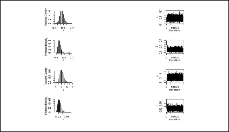
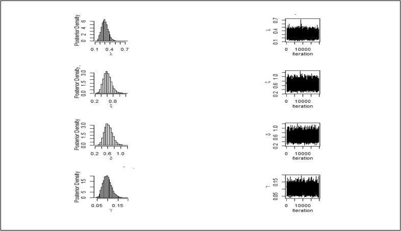
One might notice that estimates are not analytically predictable, so we also use the Adaptive Metropolis Hasting algorithm MCMC (Monte Carlo Markov Chain) to attain estimates. Fig. 12, Fig. 13 are sketched for trace plots and estimated posterior densities for Monte Carlo Markov Chain estimates of model parameters using real data sets. These figures showed the good convergence of estimates. On the other side, Table 7 provided the posterior summaries for both data sets. We provide Bayes estimates, LCL (lower credible limit), posterior variance, UCL (upper credible limit) of credible intervals. The behaviour of the estimated densities of all the parameters are slightly positively skewed.

Fig. 12.

Density plots and Trace plots of parameters $\gamma ,\delta ,\xi$ and $\lambda$ for data set I.

Fig. 13.

Density plots and Trace plots of parameters $\gamma ,\delta ,\xi$ and $\lambda$ for data set II.

Table 7.

Posterior summaries of the GLET-GTII model for data set I and II.

Data	n	Parameter	2.5%	97.5$\%$	Posterior Mean	Posterior Variance
		$\gamma$	0.228357	0.481515	0.343964	0.004009
I	30	$\delta$	0.129464	0.357515	0.220179	0.002465
		$\xi$	1.858141	4.526620	3.052603	0.380427
		$\lambda$	0.013755	0.044269	0.025770	0.000051
		$\gamma$	0.184741	0.431814	0.295535	0.004113
II	66	$\delta$	0.382319	0.876892	0.602914	0.016561
		$\xi$	0.391735	0.885013	0615787	0.015930
		$\lambda$	0.064211	0.141740	0.098712	0.000397

Implementations of real data

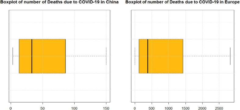
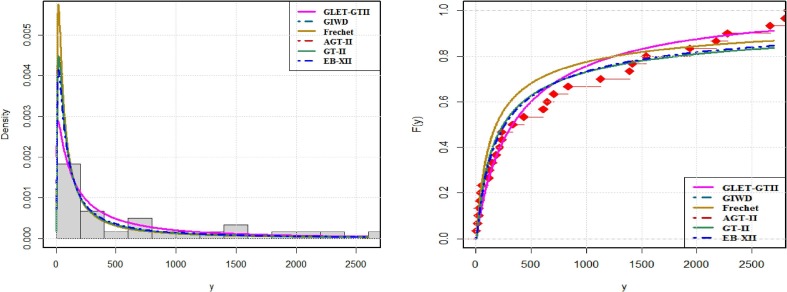
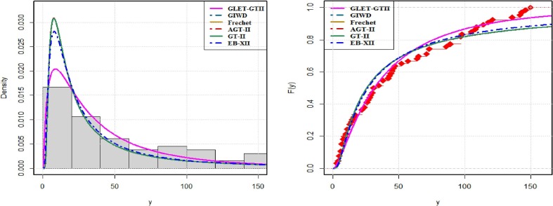
Two examples are presented here to describe the efficiency of suggested distribution. The R software is used to show the improved efficiency of GLET-GTII distribution and numerical calculations. Consider the following models (i) GIWD (generalized inverse Weibull distribution) [19] (ii) Frechet model (Frechet), (iii) Additive Gumbel Type-II (AGT-II) (iv) GT-II (Gumbel Type-II) and (v) EB-XII (Exponentiated Burr XII) model for comparative purposes. Different methodologies of segregation based on LLHF (log-likelihood function) assessed at MLEs were also taken into account: Akaike Information Criterion (AIC) computed through $\mathit{AIC}:2\left[\varsigma -L\left\{\left(\widehat{\gamma },\widehat{\delta },\widehat{\xi },\widehat{\lambda }\right)\text{;}y\right\}\right]$, and Bayesian Information Criterion $\mathit{BIC}:-2L\left\{\left(\widehat{\gamma },\widehat{\delta },\widehat{\xi },\widehat{\lambda }\right)\text{;}y\right\}+\varsigma \log \left(n\right)$, Corrected Akaike information Criterion $\mathit{AICC}=\mathit{AIC}+\frac{2\varsigma \left(\varsigma +1\right)}{n-\varsigma -1}$, Hannan Quinn Information Criterion $\mathit{HQIC}=-2L\left\{\left(\widehat{\gamma },\widehat{\delta },\widehat{\xi },\widehat{\lambda }\right)\text{;}y\right\}+2\mathit{klog}\left[\log \left(n\right)\right]$, where $\varsigma$represents the number of parameters to be fitted and $\widehat{\gamma },\widehat{\delta },\widehat{\xi },\widehat{\lambda }$ the estimates of $\gamma ,\delta ,\xi$and $\widehat{\lambda }$. The best model is the one which provides the minimum values of those benchmarks. The outputs revealed that GLET-GTII distribution is a bestest model than the abovementioned models in each case. To check whether the data fits GLET-GTII $\left(\gamma ,\delta ,\xi ,\lambda \right)$model, we use Kolmogorov–Smirnov (K-S) distances among empirical distribution function and fitted distribution function. In Table 5, Table 6 , the K-S test value and the corresponding critical value are given. The small K-S distance and the large critical-value for the test indicate that this data matches perfectly almost well with GLET-GTII $\left(\gamma ,\delta ,\xi ,\lambda \right)$model. Now standardized $\mathrm{”}\mathit{goodness}$ of $\mathit{fit}\mathrm{”}$ measures are utilized to validate which model fits these data best. Cramér-Von Mises and Anderson-Darling test statistics are taken into acount (for more detail see Chen and Balakrishnan [20]). Generally, the smallest values of Cramér-Von Mises $\left(W^{\ast }\right)$ and Anderson-Darling $\left(A^{\ast }\right)$, indicates the better fit of data. The values of the statistics $A^{\ast }$ and $W^{\ast }$ are listed inTable 5, Table 6. The summary statistics are graphed via box plots for data sets ”I and II” and shown in Fig. 7 . A very useful tool for interpreting our data is the box plot. In a single clear and concise diagram, the box plot contains all the knowledge about data. A boxplot is a systematic way to view data distribution based on a summary of five numbers (“minimum”, first quartile (Q1), median, third quartile (Q3), and “maximum”). A box plot is a visualization that provides a real indication of how the values are distributed out in the data. In Fig. 9, Fig. 10 , the estimated densities of GLET-GTII $\left(\gamma ,\delta ,\xi ,\lambda \right)$and competitor models were graphed for more visual comparison. The mentioned below data sets are given in Sindhu et al. [27]. (see Fig. 11, Fig. 8 ).

Table 5.

Values of the considered measures for Data Set I.

Distribution	GLET-GTII	GIWD	Frechet	AGT-II	GT-II	EB-XII
$W\ast$	0.10657	0.28434	0.28433	0.28444	0.28434	0.23364
$A\ast$	0.79738	1.75835	1.75829	1.75861	1.75835	1.48713
$K-S$	0.08904	0.12843	0.12845	0.12888	0.12843	0.11457
p-value	0.67210	0.22640	0.22620	0.22290	0.22640	0.35170
AIC	656.367	668.203	666.203	670.162	666.203	664.695
CAIC	657.023	668.590	666.394	670.818	666.397	665.082
BIC	665.126	674.772	670.583	678.921	670.583	671.264
HQIC	659.828	670.799	667.934	673.623	667.934	667.291

Table 6.

Values of the considered measures for Data Set II.

Distribution	GLET-GTII	GIWD	Frechet	AGT-II	GT-II	EB-XII
$W\ast$	0.06748	0.15402	0.15425	0.15404	0.15402	0.12913
$A\ast$	0.49019	0.98445	0.98601	0.98453	0.98444	0.84641
$K-S$	0.11845	0.15964	0.17716	0.15960	0.15964	0.14954
p-value	0.75020	0.38800	0.26980	0.38820	0.38790	0.46870
AIC	469.175	475.394	474.074	477.394	473.394	473.437
CAIC	470.775	476.317	474.518	478.994	473.838	474.360
BIC	474.780	479.597	476.876	482.998	476.196	477.641
HQIC	470.969	476.738	474.970	479.187	474.290	474.782

Fig. 7.

Box plots for data sets I and II.

Fig. 9.

Estimated densities (left) and cdf (right) for data set II.

Fig. 10.

The profiles of the Log-likelihood plots for the parameters of data set I.

Fig. 11.

The profiles of the Log-likelihood plots for the parameters of data set 2.

Fig. 8.

Estimated densities (left) and cdf (right) for data set I.

Data I: Daily deaths number because of COVID-19 in China {23^rd January to 28^th March}

This data is taken from given website ( https://www.worldometers.info/coronavirus/country/china/), which indicates the daily number of deaths because of COVID-19 in China. The data is given below:

$$\{8,16,15,24,26,26,38,43,46,45,57,64,65,73,73,86,89,97,108,97,146,121,143,142,105,98,136,114,118,109,97,150,71,52,29,44,47,35,42,31,38,31,30,28,27,22,17,22,11,7,13,10,14,13,11,8,3,7,6,9,7,4,6,5,3,5\}\text{.}$$

Data II:Daily deaths number because of COVID-19 in Europe {$I^{\mathit{st}}-{30}^{\mathit{th}}$ March}

This data is taken from given website (https://covid19.who.int/), which indicates daily deaths number because of COVID-19 in Europe.

$$\{6,18,29,28,47,55,40,150,129,184,236,237,336,219,612,434,648,706,838,1129,1421,118,116,1393,1540,1941,2175,2278,2824,2803,2667\}\text{.}$$

For each distribution, we estimate the unknown parameters using maximum likelihood. The MLEs with their respective standard errors of the above models are listed in Table 4 . These calculations were made using the R programming language.

Table 4.

Parameters estimates and Standard errors for both Data Sets.

		MLE	Error	MLE	Error
Model	Parameter	Data I		Data II
GLET-GTII	$\widehat{\gamma }$	0.206478	0.04659	0.14714	0.10045
	$\widehat{\delta }$	3.354146	1.96348	3.50279	2.61427
	$\widehat{\xi }$	3.354146	1.96347	3.50279	2.61427
	$\widehat{\lambda }$	134.0219	160.264	98.9773	362.710
GIWD	$\widehat{\alpha }$	9.10197	811.843	2.70212	334.481
	$\widehat{\beta }$	0.91594	0.08369	0.57051	0.07536
	$\widehat{b}$	1.78997	146.234	9.18399	648.661
Frechet	$\widehat{\eta }$	17.1868	2.45283	99.7713	29.7155
	$\widehat{\alpha }$	0.91589	0.08368	0.59186	0.07787
AGT-II	$\widehat{\beta }$	7.47910	116.202	9.79414	8033.73
	$\widehat{\lambda }$	13.4320	3.46155	6.40543	8033.75
	$\widehat{\delta }$	4.48651	6.66264	0.57062	0.11674
	$\widehat{\alpha }$	0.91372	0.09052	0.57071	0.21937
GT-II	$\widehat{\beta }$	0.91595	0.08369	0.57057	0.07536
	$\widehat{\alpha }$	13.5324	3.10943	16.1933	5.71448
EB-XII	$\widehat{\beta }$	0.42854	0.16904	0.29162	0.13471
	$\widehat{b}$	59.0695	58.8060	52.0316	54.4001
	$\widehat{\eta }$	2.74026	1.33481	2.39459	1.36109

Conclusion

Here, we have suggested a new general construction of flexible lifetime models by rendering any existing baseline model more versatile via simple transformation. A generalized log-exponential transformation model is introduced and its implementation is demonstrated by taking Gumbel Type-II model. The mathematical properties of proposed model have been analyzed in detail. Additionally, some figures for density and hazard function are included. The general non-central incomplete and complete moments are also included. Uncertainty measures such as entropies (like Renyi, Tsallis, Verma, and Kumar entropy Mathai-Houbold) are calculated. The estimation of parameters is accessed by utilizing two techniques such as maximum likelihood method and Bayesian framework. Through utilizing classical goodness of fit indicators, we evaluate the efficiency of GLET-GTII model with its five significant counterparts. The posterior densities, Log-likelihood and trace plots are drawn for considered data sets. These findings are in line with fact that proposed model is quite suitable for implementations of real life data.

Credit authorship contribution statement

Tabassum Naz Sindhu, Anum Shafiq and Qasem M. Al-Mdallal contributed to the conceptualization, design and implementation of the research, to the analysis of the results and to the writing of the manuscript.

Declaration of Competing Interest

The authors declare that they have no known competing financial interests or personal relationships that could have appeared to influence the work reported in this paper.

References

- 1.Marshall A.W., Olkin I. A new method for adding a parameter to a family of distributions with application to the exponential and Weibull families. Biometrika. 1997;84:641–652. [Google Scholar]
- 2.Gupta R.C., Gupta P.I., Gupta R.D. Modeling failure time data by Lehmann alternatives. Commun Stat Theory Methods. 1998;27:887–904. [Google Scholar]
- 3.Eugene N., Lee C., Famoye F. Beta-normal distribution and its applications. Commun Stat Theory Methods. 2002;31:497–512. [Google Scholar]
- 4.Cordeiro G.M., de Castro M. A new family of generalized distributions. J Stat Comput Sim. 2011;81:883–898. [Google Scholar]
- 5.Zografos K., Balakrishnan N. On families of beta and generalized gamma generated distributions and associated inference. Stat Methodol. 2009;6:344–362. [Google Scholar]
- 6.Aslam M., Ley C., Hussain Z., Shah S.F., Asghar Z. A new generator for proposing flexible lifetime distributions and its properties. PLoS ONE. 2020;15(4) doi: 10.1371/journal.pone.0231908. e0231908. [DOI] [PMC free article] [PubMed] [Google Scholar]
- 7.Gumbel E. Les valeurs extremes des distributions statistiques. Annales de l’Institut Henri Poincare. 1935;5(2):115–158. [Google Scholar]
- 8.Gumbel E.J. The return period of flood flows. Ann Math Stat. 1941;12:163–190. [Google Scholar]
- 9.E.J. Gumbel, Statistical Theory of Extreme Values and Some Practical Applications, vol. 33 of Applied Mathematics, U.S. Department of Commerce, National Bureau of Standards, ASIN B0007DSHG4, Gaithersburg, Md, USA, 1st ed., 1954.
- 10.Sindhu T.N., Riaz M., Aslam M., Ahmed Z. Bayes estimation of Gumbel mixture models with industrial applications. Trans Inst Meas Control. 2016;38(2):201–214. [Google Scholar]
- 11.Sindhu T.N., Feroze N., Aslam M. Study of the left censored data from the gumbel type II distribution under a bayesian approach. J Modern Appl Statist Methods. 2016;15(2):1–10. [Google Scholar]
- 12.European Centre for Disease Prevention and Control. “Situation Update—Worldwide. 2020. Available online:https://www.ecdc.europa.eu/en/geographical-distribution-2019-ncov-cases [accessed on 13 February 2020].
- 13.Wang C, Horby PW, Hayden FG, et al. A novel coronavirus outbreak of global health concern. Lancet (London, England); 2020. [DOI] [PMC free article] [PubMed]
- 14.Huang C., Wang Y., Li X. Clinical features of patients infected with 2019 novel coronavirus in Wuhan, China. Lancet. 2020;395:497–506. doi: 10.1016/S0140-6736(20)30183-5. [DOI] [PMC free article] [PubMed] [Google Scholar]
- 15.World Health Organization. Novel Coronavirus (2019-nCoV) Situation Report – 14. Available online:https://www.who.int/docs/default-source/coronaviruse/situationreports/20200203-sitrep-14-ncov.pdf?sfvrsn=f7347413_4. February 3rd, 2020.
- 16.Silva G.O., Ortega E.M.M., Cordeiro G.M. The beta modified Weibull distribution. Lifetime Data Anal. 2010;16:409–430. doi: 10.1007/s10985-010-9161-1. [DOI] [PubMed] [Google Scholar]
- 17.Ross S.M. 2nd ed. Wiley; New York: 1996. Stochastic processes. [Google Scholar]
- 18.Mathai A.M., Haubold H.J. On a generalized entropy measure leading to the pathway model with a preliminary application to solar neutrino data. Entropy. 2013;15(10):4011–4025. [Google Scholar]
- 19.De Gusmao F.R., Ortega E.M., Cordeiro G.M. The generalized inverse Weibull distribution. Stat Pap. 2011;52(3):591–619. [Google Scholar]
- 20.Chen Gemai, Balakrishnan N. A general purpose approximate goodness-of-fit test. J Qual Technol. 1995;27(2):154–161. doi: 10.1080/00224065.1995.11979578. [DOI] [Google Scholar]
- 21.Sindhu T.N., Hussain Z. Predictive inference and parameter estimation from the half-normal distribution for the left censored data. Ann. Data. Sci. 2020 doi: 10.1007/s40745-020-00309-6. [DOI] [Google Scholar]
- 22.Sindhu T.N., Hussain Z. Mixture of two generalized inverted exponential distributions with censored sample: properties and estimation. Statistica Applicata – Italian J Appl Stat. 2018;30(3):373–391. doi: 10.26398/IJAS.0030-019. [DOI] [Google Scholar]
- 23.Sindhu T.N., Aslam M., Shafiq A. Bayesian Analysis of two Censored Shifted Gompertz Mixture Distributions using Informative and Noninformative Priors. Pakistan J Stat Oper Res. 2017:227–243. [Google Scholar]
- 24.Sindhu T.N., Aslam M., Hussain Z. A simulation study of parameters for the censored shifted Gompertz mixture distribution: a Bayesian approach. J Stat Manage Syst. 2016;19(3):423–450. [Google Scholar]
- 25.Sindhu T.N., Khan H.M., Hussain Z., Lenzmeier T. Bayesian prediction from the inverse rayleigh distribution based on type-II trim censoring. J Stat Manage Syst. 2017;20(5):995–1008. [Google Scholar]
- 26.Sindhu T.N., Hussain Z., Aslam M. Parameter and reliability estimation of inverted Maxwell mixture model. J Stat Manage Syst. 2019;22(3):459–493. [Google Scholar]
- 27.Sindhu TN, Shafiq A, Al-Mdallal QM. Exponentiated transformation of Gumbel Type-II distribution for modeling COVID-19 data. Alexand Eng J (accepted); 2020.https://doi.org/10.1016/j.aej.2020.09.060.