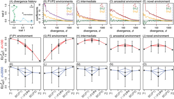
Figure 4.

The outcomes of hybridization over time and space. (A) A cartoon of the divergence process that was simulated, with two populations adapting in allopatry to abruptly shifting optima, and then continuing to accumulate divergence via system drift. (B)–(E) change in the composite effects with increasing divergence (Table 1), as measured with respect to (B) both parental environments, or (C)–(E) other single environments. (F)–(O) results for simulated hybrids, plotting $r_{\mathrm{HO}}^2$ on a reversed axis, such that fitter genotypes are higher. Points with error bars show the mean and 95% quantiles for 10,000 recombinant hybrids, generated for the reciprocal backcrosses, and the $\mathrm{F}2$. The dark central point (labeled Fn) shows the mean of 10,000 homozygous hybrids, derived from automictic selfing among F1 gametes. Red and blue lines show analytical predictions. These use equation (17), with the measured values of $r_{1\mathrm{O}}^2$ and $r_{2\mathrm{O}}^2$, and the assumption that $\rho =-1$ (for the “intermediate” environment) or $\rho =0$ (all other cases). Hybrids were scored in the (F)–(J) early stages of divergence ($d=100$; red lines), and (K)–(O) at later stages ($d=2000$; blue lines). Simulation procedure is described in Supporting Information Appendix 2, and used the following parameters: $N=1000$, $N\overline{s}=-10$, $2NU=1$, $n=2$, $k=2$, free recombination, and “bottom‐up” mutations.