

Abstract
Transfer entropy (TE) is a recently proposed measure of the information flow between coupled linear or nonlinear systems. In this study, we suggest improvements in the selection of parameters for the estimation of TE that significantly enhance its accuracy and robustness in identifying the direction and the level of information flow between observed data series generated by coupled complex systems. We show the application of the improved TE method to long (in the order of days; approximately a total of 600 h across all patients), continuous, intracranial electroencephalograms (EEG) recorded in two different medical centers from four patients with focal temporal lobe epilepsy (TLE) for localization of their foci. All patients underwent ablative surgery of their clinically assessed foci. Based on a surrogate statistical analysis of the TE results, it is shown that the identified potential focal sites through the suggested analysis were in agreement with the clinically assessed sites of the epileptogenic focus in all patients analyzed. It is noteworthy that the analysis was conducted on the available whole-duration multielectrode EEG, that is, without any subjective prior selection of EEG segments or electrodes for analysis. The above, in conjunction with the use of surrogate data, make the results of this analysis robust. These findings suggest a critical role TE may play in epilepsy research in general, and as a tool for robust localization of the epileptogenic focus/foci in patients with focal epilepsy in particular.
Index Terms—: Epilepsy, epileptogenic focus localization, information flow, transfer entropy (TE)
I. Introduction
Research in the field of nonlinear dynamics has recently focused upon the analysis of data from coupled nonlinear systems [1], [2]. The identification of the direction of information flow and estimation of the strength of interaction between data series from such systems, especially when their structure is unknown, hold promise for the understanding of the mechanisms of their interactions, and for a subsequent design and implementation of appropriate schemes to control a possibly erratic behavior these and similar systems in nature may exhibit over time. A relevant example is the epileptic brain and the intermittent occurrence of epileptic seizures.
Commonly used tools for the estimation of linear dependencies between data series are the linear cross-correlation in the time domain and the cross-coherence in the frequency domain [3]. A mathematically more general (nonparametric, model-free) and statistically rigorous approach for the detection of linear and nonlinear interdependences between time series is the mutual information (MI). However, MI being a symmetrical function with respect to its arguments, cannot detect directional flow of information and causal relationships unless one of the time series is time delayed. Although the introduction of a time delay in MI is an important improvement to this goal, the resulting measure presents a set of difficulties. One important issue is that its estimation requires a relatively large amount of high quality data (noise-free, stationary, that is, characteristics rarely met in real world data where experimental signals are typically short, nonstationary and likely to be masked at least by measurement noise), especially if the causal effect under investigation is weak. A second issue is the poor sensitivity and specificity of MI to existing and/or nonexisting delays in the causal structure of the analyzed time series, respectively [4].
To study the directional aspect of interactions, many other approaches have been employed [4]–[9]. One of these approaches is based on the improvement of the prediction of a series’ future values by incorporating information from another time series. Such an approach was originally proposed by Wiener [6] and later formalized by Granger in the context of linear regression models of stochastic processes. Granger causality was then extended to nonlinear systems by 1) applying to local linear models in reduced neighborhoods, estimating the resulting statistical quantity and then averaging it over the entire dataset [4], or 2) considering an error reduction that is triggered by added variables in global nonlinear models [5].
Despite the relative success of the above approaches in detecting the direction of interactions in special cases, they essentially are model-based (parametric) methods (linear, as well as nonlinear), i.e., either make assumptions about the structure of the interacting systems or the nature of their interactions, and as such they may suffer from the shortcomings of modeling systems/signals of unknown structure. For a detailed review of parametric and nonparametric(linear, as well as nonlinear) measures of causality, we refer the reader to [10] and [11]. To overcome this problem, an information theoretic approach to identify the direction of information flow and quantify the strength of coupling between complex systems/signals has recently been suggested [7]. This method was based on the study of transitional probabilities of the states of systems/signals under consideration. The resulted measure was termed Transfer Entropy (TE).
We have shown [8], [9] that the direct application of the method as proposed in [7] may not always give the expected results, and that tuning of certain parameters involved in the TE estimation plays a critical role in detecting the correct direction of the information flow between time series. We herein propose a methodology to also test the significance of the TE values using surrogate data analysis. We then employ the improved TE method to define three new measures, the net transfer entropy NTE, the spatial average net transfer entropy (SANTE) and the temporal probability distribution (PD) of SANTE in a study for localization of the epileptogenic focus.
The organization of the rest of this paper is as follows. The measure of TE, the improvements, practical adjustments and new measures we introduced, are described in Section II. In Section III, the application of these measures to EEG for identification of the epileptogenic focus is presented. Discussion of these results and conclusions are given in Section IV and V, respectively.
II. Methodology
A. Transfer Entropy
Consider a kth-order Markov process [12] described by
| (1) |
where P is the conditional probability of a random process X being in state xn+1 at time n + 1. Equation (1) implies that the probability of occurrence of a particular state xn+1 depends only on the past k states of the system. The definition given in (1) can be extended to the case of Markov interdependence of two random processes X and Y as
| (2) |
where are the past l states of the second random process Y. This generalized Markov property implies that the state xn+1 of the process X depends only on the past k states of the process X and not on the past l states of the process Y. However, if the process X also depends on the past states (values) of process Y, the divergence of the hypothesized (a priori) transition probability, [left-hand side of (2)], from the true underlying transition probability of the system, [right-hand side of (2)] can be quantified using the Kullback–Leibler measure [13]. Thus, the Kullback–Leibler measure quantifies the TE from the driving process Y to the driven process X, and it is given by
| (3) |
The values of the parameters k and l are the orders of the Markov process for the two coupled processes X and Y, respectively. The value of N denotes the total number of the available points per process in the state space.
A simple manipulation of (3) permits a decomposition of the transfer entropy in terms of conditional entropies [14] and justifies the use of TE as a measure of information flow from Y to X:
| (4) |
where is the information gained about the future state xn+1 by using the information from (i.e., the past k states of X), and is the information gained about the future state xn+1 by using the information from (i.e., the past l states of Y) in addition to . Thus, TE(Y → X) is the additional information gained from process Y about the future state of the process X, and therefore it can be seen as the information flow from the process Y to process X. Equation (4) also implies that when the processes X and Y are independent, the value of TE(Y → X) is zero.
In search of optimal k, it would generally be desirable to choose the parameter k as large as possible in order to find an invariant value (e.g., for conditional entropies), but in practice the finite size of any real dataset imposes the need to find a reasonable compromise between finite sample effects and approximation of the actual value of probabilities. Therefore, the selection of k and l plays a critical role in obtaining reliable values for the TE from real data. In addition, the estimation of TE also depends on the neighborhood size (radius r) used in the state space for the calculation of the involved joint and conditional probabilities. The value of radius r in the state space defines the maximum norm distance in the search for neighboring state space points. The involved probabilities are not accurately estimated for large r values, and may eventually lead to erroneous estimates of TE.
B. Improved Computation of TE
Selection of k: The value of k (order of the driven process) used in the calculation of TE(Y → X) [see (3)] represents the dependence of the state xn+1 of the system on its past k states. A classical linear approach to autoregressive (AR) model order selection, namely the Akaike information criterion (AIC), has been applied to the selection of the order of Markov processes. Evidently, AIC suffers from substantial overestimation of the Markov process order in nonlinear systems and therefore is not a consistent estimator [15]. Arguably, a method to estimate this parameter is the delayed mutual information [16]. The delay d at which the mutual information of X reaches its first minimum can be taken as the estimate of the period within which two states of X are dynamically correlated with each other. In essence, this value of d minimizes the Kullback–Leibler divergence between the dth and higher order corresponding probabilities of the driven process X [see (1)], i.e., there is minimum information gain about the future state of X by using its values that are more than d steps in the past. Thus, in units of the sampling period, d would be equal to the order k of the Markov process. If the value of k is severely underestimated, the information gained about xn+1 will erroneously increase due to the presence of yn, and would result to an incorrect estimation of TE. A straightforward extension of this method for estimation of k from real-world data may not be possible, especially when the selected value of k is large (i.e., the large embedding dimension of state space for finite duration data in the time domain) [14]. This may thus lead to an erroneous calculation of TE. Therefore, from a practical point of view, a statistic that may be used is the correlation time constant te, which is defined as the time required for the autocorrelation function (AF) to decrease to 1/e of its maximum value (maximum value of AF is 1) [16]. AF is an easy metric to compute over time, it has been found to be robust in many simulations, but it only detects linear dependencies in the data. Despite the latter drawback, we have used AF to approximately estimate k per data segment generated either from simulation models or the epileptic brain. We would like to emphasize that estimation of k was conducted per data segment under consideration (e.g., 10.24 s of EEG per electrode site in the epilepsy application). As we show below and elsewhere [8], [9], the derived results for the detection of the direction and level of interactions justify such a compromise in the estimation of k.
Selection of l: The value of l (order of the driving system) was chosen to be equal to 1. The justification for the selection of this value for l is the assumption that the current state of the driving system is sufficient to produce a considerable change in the dynamics of the driven system within one time step (and hence only immediate interactions between X and Y are assumed to be detected in the analysis herein). When larger values for l were employed (i.e., a delayed influence of Y on X), detection of information flow from T to X was possible too. These latter results are not presented in this paper.
-
Selection of Radius r: The multidimensional transitional probabilities involved in the definition of TE [(3)] are calculated by joint probabilities using the conditional probability formula P(A|B) = P(A, B)/P(B). One can then reformulate the TE as
(5) From the above formulation, it is clear that probabilities of a vector in the state space at the nth time step are compared with ones of vectors in the state space at the (n+1)th time step, and therefore the units of TE are in bits/time step, where time step in simulation studies is the algorithm’s (e.g., Runge–Kutta) iteration step. In real life applications (like in the EEG) the time step corresponds to the sampling period of the sampled (digital) data. The multidimensional joint probabilities in (5) are estimated through the generalized correlation integrals Cn(r) in the state space of embedding dimension P = k + l + 1[17] as
where Θ(x > 0) = 1, Θ(x = 0) = 0, |·| is the maximum distance norm, and the subscript (n+1) is included in C to signify the dependence of C on the time index n [note that averaging over n occurs in the estimation of TE, using (6) into (3)]. In the rest of the paper we use the notation Cn(r) or Cn+1(r) for C interchangeably. Equation (6) is in fact a simple form of a kernel density estimator where the kernel is the Heaviside function Θ. We found that the use of a more elaborate kernel (e.g., a Gaussian or one which takes into account the local density of the states in the state space) than the Heaviside function does not necessarily improve the ability of the measure to detect direction and strength of coupling. In order to avoid a bias in the estimation of the multidimensional probabilities, temporally correlated pairs of points are excluded from the computation of Cn(r) by means of the Theiler correction and a window of (p − 1) * l = k in duration [18].(6) The estimation of joint probabilities between two different time series requires concurrent calculation of distances in both state spaces [see (5)]. Therefore, in the computation of Cn(r), the use of a common value r* of radius r in both state spaces is desirable. In previous publications ([8], [9]), using simulation examples (unidirectional as well as bidirectional coupling in two and three coupled oscillator model configurations), we have found that the TE values obtained for only a certain range of r accurately detect the direction and strength of coupling. Typically, these r values corresponded to the ones for which we observed a quasi-linear region in the ln Cn(r) versus ln r curve [19]. Although such an estimation of r* is possible in noiseless simulation data, for physiological data sets that are always noisy and the underlying functional description is unknown, it is difficult to estimate an optimal value r* simply because a linear region of ln Cn(r) versus ln r may not be apparent. It is known that for small r values, the presence of noise in the data will be predominant [20], [21] and over the entire space (high-dimensional). This causes the distance between neighborhood points to increase. Consequently, the number of neighbors available to estimate the multidimensional probabilities at the smaller scales may decrease and it would lead to a severely biased estimate of TE. On the other hand, at large values of r, a flat region in ln Cn(r) may be observed (saturation). In order to avoid the above shortcomings in the practical application of this method (e.g., on EEG), we approximated TE as the average of TEs estimated over an intermediate range of values (from σ/5 to 2σ/5; where σ is the standard deviation of the raw, time series data). The decision to use this range for r was made on the practical basis that r less than σ/2 typically (well-behaved data) avoids saturation and r larger than σ/10 typically filters a large portion of A/D generated noise (simulation examples offer corroborative evidence for such a claim). Even though these criteria are soft (no exhaustive testing of the influence of the range of r on the final results was performed herein), it appeared that the proposed range for r constitutes a very good compromise (sensitivity and specificity-wise) for the subsequent detection of the direction and magnitude of flow of entropy.
C. Statistical Significance of TE
The statistical significance of the values of TE was tested using the method of surrogate analysis. Since TE calculates the direction of information transfer between systems by quantifying their conditional statistical dependence, a random shuffling applied to the original driver data series (e.g., Y) destroys the temporal correlation and significantly reduces the information flow TE(Y → X). Thus, in order to estimate the statistically significant values of TE(Y → X), the null hypothesis that the current state of the driver process Y does not contain any additional information about the future state of the driven process X was tested against the alternate hypothesis of a significant time dependence between the future state of X and the current state of Y. One way to achieve this is to compare the estimated values of TE(Y → X) (i.e., the ), thereafter denoted by TEo, with the TE values estimated by studying the dependence of future state of X on the values of Y at randomly shuffled time instants (i.e., ), thereafter denoted by TEs, where p ∈ 1, … , N is selected from the shuffled time instants of Y. The above described surrogate analysis is valid when l = 1; for l > 1, tuples from original Y, each of length l, should be shuffled instead.
The shuffling was based on generation of white Gaussian noise and reordering of the original data samples of the driver data series according to the order indicated by the generated noise values (i.e., random permutation of all indices 1, … , N and reordering of the Y time series accordingly). Transfer entropy TEs values of the shuffled datasets were calculated at the “optimal” values of r from the original data. If the TE values obtained from the original time series (TEo) were greater than Tth standard deviations from the mean of the TEs values, the null hypothesis was rejected at the α = 0.01. level. (The value of Tth depends on the desired level of confidence 1 – α, and the number of the shuffled data segments generated, that is, the degrees-of-freedom of the test.)
D. Detecting Causality Using Transfer Entropy
Since it is difficult to expect a truly unidirectional flow of information in real-world data (where flow is typically bidirectional), we have defined a causality measure we called NTE that quantifies the driving of Y by X as
| (7) |
Positive values of NTE(Y → X) denote that Y drives (causes) X, while negative values denote the reverse case. Values of NTE close to zero may imply either equal bidirectional flow or no flow of information, where the values of TE will help decide between these two plausible scenarios.
III. Application to Epilepsy
Epilepsy is a disorder of the brain with intermittent occurrences of transitions to seizures, that is, massive electrical discharges that usually propagate from a focal pathological area to normal sites of the brain and disrupt its normal operation [22]. Thus, significant alteration of information flow is expected to occur ictally (during seizures), as well as possibly interictally (between seizures).
An epileptogenic focus (also called focal zone in the medical literature to include the possibility of a larger spatial extent than the one the available recording electrodes can record from, as well as to denote involvement of more than one brain structures) is electrophysiologically defined as the brain’s area that first (resolution of seconds to milliseconds) exhibits the electrographical onset of epileptic seizures [23]. The EEG signals are very helpful in providing evidence for epilepsy, but their visual inspection is often not reliable in identifying the epileptogenic focus, especially in the presence of artifacts and when there is a not well-defined spread of the epileptoformic activity. The primary objective in presurgical evaluation of patients, who are candidates for ablative surgery for the treatment of epilepsy, is to identify the region responsible for generating the patient’s habitual seizures. Usually, resection of the focal tissue is sufficient to substantially reduce or permanently abate epileptic seizures in carefully selected uni-focal patients [24]. The hypothesis we consider herein is that the epileptogenic focus acts as the driver (source of information) for the normal brain sites that participate in a seizure activity (sink of information) over extensive periods of time. One could then identify the epileptogenic focus as the brain site or sites that mostly and for a prolonged period drive the rest of the brain. We apply the TE methodology to quantitatively test this hypothesis in patients with clinically well-defined focus/foci in the temporal lobe (amygdala, hippocampus, cerebral cortex).
A. Recording Procedure and EEG Data
Only a few studies have examined the information flow changes in the epileptic brain. Most of these studies have been single-center studies with a limited number of patients analyzed, of a very limited duration and selectively analyzed EEG recordings per patient and study, and more importantly, only homologous structures in the two brain hemispheres (e.g., left versus right hippocampus; [25], [26]). In this paper, we test our methodology on EEG data from two distinct epilepsy centers, namely the Shands Hospital, Gainesville, FL, and the Barrow Neurological Institute, Phoenix AZ, that use different recording electrode montages. Four patients (two from each center), who underwent presurgical evaluation via long-term intracranial EEG recordings and subsequent successful (Engel’s class I, [24]) surgery with removal of the clinically identified epileptogenic focus, were chosen for dynamical analysis of their stored presurgical, long-term, continuous EEG recordings of days in duration (more than 600 h—see Table I). Informed consent for participation in this study was obtained from all patients. The recording procedures and characteristics of the recorded EEG data are further described below.
TABLE I.
Patients and EEG Data Characteristics
| Patient ID | Number of available intrcranial electrodes | Duration of EEG recording (hours) | Number of seizures in the EEG data | Focus (Clinical assessment) |
|---|---|---|---|---|
| 1 | 28 | 200.2 | 24 | Right Hippocampus (RTD) |
| 2 | 28 | 143.4 | 18 | Right Hippocampus (RTD) |
| 3 | 40 | 113.6 | 24 | Left Amygdala (LA) |
| 4 | 40 | 168.4 | 29 | Left Amygdala (LA) |
EEG From Shands Teaching Hospital, Gainesville, Florida [See Fig. 1(a)] : The two patients (Patients 1 and 2) from this medical center underwent a stereotactic placement of bilateral depth electrodes in the hippocampi (RTD electrode strip in the right hippocampus with RTD6 posterior, and RTD1 anterior and adjacent to right amygdala; LTD eelctrode strip in the left hippocampus with LTD6 posterior, and LTD1 anterior and adjacent to the left amygdala). In addition, two subdural electrode strips, LOF and ROF were placed bilaterally over the orbitofrontal lobes (LOF1 to LOF4 in the left and ROF1 to ROF4 in the right lobe; LOF1, ROF1 being most mesial and LOF4, ROF4 most lateral). Finally, two subdural electrode strips, LST and RST were placed bilaterally over the temporal lobes (LST1 to LST4 in the left and RST1 to RST4 in the right; LST1, RST1 being more mesial and LST4 and RST4 being more lateral). The video/EEG recording was performed using the Nicolet BMSI 4000 EEG machine. EEG signals were recorded using an average common reference with band pass filter settings of 0.1–70 Hz. The data were sampled at 200 Hz with a 10-bit quantization.
EEG From Barrow Neurological Institute, Phoenix, Arizona [See Fig. 1(b)]: The two patients (Patients 3 and 4) from this center underwent stereotactic placement of depth electrodes using the Kelly frame system under MRI guidance. 8-contact flexible Adtech depth electrodes with custom spacing were placed, with bilaterally symmetric positioning, in amygdala (LA and RA), mid hippocampus (LH, RH), orbitofrontal areas (LO, RO), and in frontal cortex (LF and RF) from superior sagittal region near supplementary motor area and cingulate (higher electrode numbers denote a more posterior location). For all electrodes, contacts #1 were mesial and contacts #8 were most distal. Electrodes in the temporal lobe were oriented orthogonally to temporal bone, allowing sampling of limbic (contacts 1–4) and temporal neocortical structures (contacts 5–8). There was a 0.5 cm distance between electrodes. Video/EEG monitoring was performed using the Nicolet BMSI 6000 EEG machine. EEG signals were recorded with an average common reference, using amplifiers with an input sensitivity range of 0–200 μV/mm and a frequency range of 0.5–70 Hz. Prior to storage, the data were sampled at 400 Hz using an analog to digital (A/D) converter with 12-bit quantization.
Fig. 1.

Schematic diagram showing depth and subdural electrode placement. The electrode montages used for recording EEG signals (a) at Shands Hospital, Gainesville, FL and (b) at Barrow Neurological Institute, Phoenix, AZ (see text for description of acronyms of the electrode positions).
B. TE and its Application to EEG for Localization of the Epileptogenic Focus
In the analysis of EEG signals, we kept the l-Markov order of the driving system equal to 1, to mainly investigate direct (not delayed) interactions between involved subsystems. As an estimate of the k-Markov order of the driven system, for each (sequential in time) 10.24 s pair of EEG segments analyzed over the complete space of electrode pairs, we used the previously described correlation time constant. To avoid searching for an elusive value r* of the radius per EEG segment, we averaged the TE values estimated over intermediate values of r within the range [σ/5 < in r < 2σ/5].
TE was estimated from successive, nonoverlapping, electrocorticographic (ECoG) and depth EEG segments of 10.24 s in duration (2048 points per segment at 200 Hz sampling rate, and 4096 points per segment at 400 Hz sampling rate) for days of EEG recording per patient. Two values of TE, one in each direction (i → j or j → i), were estimated for every electrode pair (i, j) per 10.24 s of EEG segment.
Subsequently, per EEG segment, we estimated the NTE(i → j) [see (7)] from the TE(i → j) values for each electrode pair (i, j) with j ≠ i. It is to be noted that NTE(i → j) may attain only one value (positive if information flow from (i → j) exceeds the one from (j → i), and negative otherwise) per EEG segment positioned at a time point t. The null hypothesis that the thus obtained values of NTE per electrode site i are not statistically significant was then tested. Net TE values from the shuffled EEG datasets (NTEs) were obtained per electrode and EEG segment. If an NTEo value (i.e., from analysis of the original EEG time series) was greater than Tth = 2.94 standard deviations from the mean of the NTEs values, the null hypothesis was rejected at α = 0.01 for this EEG data segment (14 degrees-of-freedom; 15 surrogate sets were generated per EEG data segment to speed up calculations—no significant differences in focus localization results were observed due to this relatively small number of generated surrogate data).
Then, in each EEG segment, the average of the statistically significant NTE per electrode site i over j was estimated, that is, the average of the values of the statistically significant NTE(i → j), in pairs (i, j) where electrode site significantly drives (sends information to) site j. We have called this spatial average of the statistically significant interactions at the level of the net TE within (t, t + 10.24 s), the spatial average net transfer entropy (SANTEt(i)) at electrode site i and time t, and we defined it as
| (8) |
where are statistically significant NTEs, that is, they satisfy the condition , where |·| denote absolute value and and are, respectively, the mean and standard deviation of the 15 NTEs values generated per 10.24 s EEG segment at time t, Tth is the threshold of 99% significance (Tth = 2.94), and N here represents the total number of available electrodes for analysis.
For illustration purposes, we plot SANTEt(i) per electrode i and 10.24 s EEG segment over 3 h for Patient 1 in Fig. 2(a), and over 6 h for Patient 2 in Fig. 2(b). From Fig. 2(a) we have a strong indication that SANTE values are large in the focal area (RTD2, RTD3 in this patient) even in the interictal period, and thus it constitutes supporting evidence about the hypothesis that the epileptogenic focus is the driver of information flow in the epileptic brain. Since the patients typically experience multiple seizures over relatively short period in the epilepsy monitoring units (EMUs), one can postulate that the consistently high values of focal driving during the interictal period marks a continued existence of an active underlying pathology. However, that was not the case for Patient 2. From Fig. 2(b) it is clear that SANTE, without any meta-processing, does not unequivocally localize the focal zone in Patient 2.
Fig. 2.

Long-term dynamics of SANTE per electrode site over time for epileptogenic focus localization in a 4 h EEG from Patient 1 (left panel), a 6 h EEG from Patient 2 (right panel). The two vertical lines in the right panel denote seizures of 2–3 min in duration. Highest values of SANTE persist for a long period at the focal zone of Patient 1 (Right temporal lobe: RTD2, RTD3). The epileptogenic zone is not clear for Patient 2 and metaprocessing was deemed necessary.
Algorithm for Focus Localization
- Step 1: The hypothesis that the epileptogenic focus drives other brain sites for the longest period of time was tested by first estimating the probability PD(i) that site i drives other brain sites j within a time interval T as equal to the normalized fraction of the period T where SANTEt(i) is positive. Thus, a maximum likelihood estimate of the driving probability of each electrode i is thus estimated as
where Θ is the Heaviside function and NT denotes the total number of 10.24 s EEG segments within the considered period T.(9) -
Step 2: The outliers of the driving probability density function PD(i) will be those electrodes that significantly drive the other electrodes for a longer period of time. An outlier detection method, that does not make any distributional assumptions, utilizes Chebyshev’s inequality to calculate the detection threshold Tu [27]. Since we are interested in identifying candidate electrodes that have high values of PD, Tu can be calculated as an upper bound on this distribution. A PD value higher than Tu is considered to be an outlier. The Chebyshev’s inequality that gives a bound for the probability of the data that fall out-side k standard deviations from the mean, is
where μ is the mean (sample mean is used to approximate μ), σ is the standard deviation (approximated by the sample standard deviation s), and k is the number of standard deviations of interest.(10) The calculation of Tu is a two-stage process. Stage 1 is used to remove possible outliers from the calculation of mean and standard deviation in the Chebyshev inequality. Stage 2 uses the distribution of the truncated data from Stage 1 to calculate the mean and standard deviation of the distribution. A value p = 0.01 for the one-tail probability for Stage 2 is chosen. Following (10), the value of k is determined and Tu is then calculated as(11) The obtained Tu value is then applied to the original distribution PD to identify outliers. All electrodes i that have values of PD(i) > Tu are marked as candidate focal electrodes (outliers). In this Step, to avoid in-sample bias in the estimation of Tu for each patient, the PD(i) estimated over the first half of the EEG record (training data set) were used to calculate Tu according to the procedure delineated above. This value of Tu, was then used to detect outliers in the PD(i) estimated from the rest (testing portion) of the EEG dataset for each patient.
Step 3: If the electrodes selected from Step 2 reside in one hemisphere, the focus is lateralized. However, if the selected electrodes reside in both hemispheres, the focus cannot be lateralized and recommendation for unilateral surgical resection cannot typically be reached. In the case of existence of dependent foci (e.g., primary and secondary), that reside in different hemispheres, the primary focus would by definition drive the secondary one (NTE of the primary focus should then be significantly larger than the one of the secondary focus). In addition, one would expect that each focus would drive electrodes in the hemisphere it resides more than ones in the contralateral hemisphere (focus/hemisphere assumption). In the case of independent foci, one focus should not significantly drive the other (i.e., the NTE between the two foci should not be statistically different). In an attempt to further investigate such a situation with two selected (independent or dependent) foci in different hemispheres, and based on the above described focus/hemisphere assumption, we developed a final Step in our epileptogenic focus localization algorithm. In this step (Step 3), we recalculate the SANTE(i) and PD(i) measures for each site i selected as outlier in Step 2. However, we now estimate the SANTE’s spatial average of NTEs only over sites j (j ≠ i) that reside in the same hemisphere as site i does (ipsilateral hemisphere). We have called the thus derived intra-hemispheric PD. We estimate over the entire data using sequential nonoverlapping 6 h EEG epochs (i.e., one value per 6 h EEG epoch). The final results in this study did not critically depend on the 6 h length of the EEG epochs. Finally, we rank all sites i entered in Step 3 according to their respective values (using nonparametric Mann–Whitney’s U test). Thus, candidate focal sites from Step 2 are further refined with respect to their focality in this Step 3.
C. Focus Localization Results
Fig. 3 shows the distribution PD(i) at each electrode i estimated for each of the 4 patients enrolled in this study. (Each PD(i) was estimated from nonoverlapping 6 h epochs over the whole testing portion of the EEG record per patient.) The threshold Tu (horizontal line in this figure) was estimated from the training portion of the EEG record per patient using the approach described previously in Step 2. All candidate focal electrodes, that is, the ones with PD larger than Tu, are shown with grey vertical bars.
Fig. 3.

Epileptogenic focus localization via the probability PD of SANTE(i) over the testing (second half of the entire recording) EEG per electrode i and patient. The grey vertical bars indicate the electrode sites selected as focal sites by the procedure in Step 2 that detects outliers in the PD(i)’s graph above. The horizontal lines denote the estimated value Tu of from the PD(i) in the first half of the data of the EEG recording per patient (see text for details).
The candidate focal electrodes obtained per patient from Step 2 are listed in column 3 of Table II. The results indicate that the candidate focal electrode sites are in very good agreement with the ones determined clinically by the physicians as focal sites (see column 2, Table II) in three out of four patients (Patients 1, 3, and 4). In these three patients, the corresponding PD values of the candidate focal electrodes were in the range 0.50–0.79. Therefore, it appears that the candidate focal electrodes have a significantly positive net information flow (NTE) towards all other electrodes they interact with for a long period of time (50%–79% of the days-long testing EEG dataset per patient). The agreement of the identified focus with the one derived from the clinical assessment supports our hypothesis that focal electrodes are the most active and most frequent drivers in the epileptic brain information-wise. [It is noteworthy that the alternate hypothesis that focus is an information sink could not localize the focus in any of the patients—results not shown here.] Interestingly, the range of PD values of the focus also suggests that the focal electrodes drive “normal” electrodes even at other times than just during seizures (which here are approximately 2 min in duration) or periods before seizures onset (typically seconds in duration for clinical assessment of the focal zone). For example, in Patient 1, we found that PD for the focal electrode RTD2 is 0.69, which means that RTD2 is the most prominent driver of brain sites for approximately 69 h within the 100.1 h testing EEG dataset in this patient.
TABLE II.
Epileptogenic Focus Localization by SANTE Versus Clinical Assessment
| Patient ID | Focus (Clinical Assessment/Clinical Outcome) | Focus Localization (PD) | Focus Lateralization / Focus Localization () |
|---|---|---|---|
| 1 | Right Temporal lobe (RTD: RTD2, RTD3) | Right Temporal lobe (RTD2) | Right hemisphere Right Temporal lobe (RTD2) |
| 2 | Right Temporal lobe (RTD: RTD3, RTD4) | Right/Left Temporal lobe (RTD3, LST3) | Right+Left hemisphere Right/Left Temporal lobe (RTD3 > LST3) |
| 3 | Left Temporal lobe (LA: LA1, LA2, LA3) | Left Temporal lobe (LA1, LA2) | Left hemisphere Left Amygdala (LA1 > LA2) |
| 4 | Left Temporal lobe (LA: LA1, LA2, LA3) | Left Temporal lobe (LA1, LA2, LA3) | Left hemisphere Left Amygdala (LA1> LA2> LA3) |
>decreasing order of driving at P <0.001(Mann-Whitney U test)
In Patient 2, in addition to RTD3, which was within the clinically determined focal zone for this patient, another candidate focal electrode was determined to be LST3. This patient had a poorer postoperative outcome (seizures were not totally abated). Interestingly, the PDs of the candidate focal electrodes in this patient were lower (between 0.43 and 0.48) than the ones in the other patients. To examine the possibility of existence of two foci (dependent or independent), we proceeded to estimate the intra-hemispheric for each of the two candidate focal electrodes LST3 and RTD3, following the procedure described in Step 3 of Section-III-B.
Determining Intra-Hemispheric Driving of Candidate Focal Electrodes: RTD3 exhibits a significantly higher intra-hemispheric than LST3 at α = 0.001 (one-tailed nonparametric Mann–Whitney U test). This means that the rate of the net information outflow of RTD3, towards the rest of the electrode sites in the right hemisphere, is significantly larger than the corresponding one of LST3 towards the electrode sites in the left hemisphere [see Fig. 4(a)]. Therefore, according to our assumption, we conclude that RTD3 resides in the zone of a major focus, which is in agreement with the clinical assessment, and LST3 in the zone of a minor focus in this patient.
Determining Inter-Hemispheric Driving of Candidate Focal Electrodes: If we extend the analysis one step further, we are able to characterize the foci identified in Patient 2 as dependent (primary or secondary), or “independent” foci. In terms of our methodology, a consistent way to do this is to compare the net transfer of entropy NTE* estimated over each of the 23 6-h EEG segments and only between two electrodes, RTD3 and LST3.
Fig. 4.
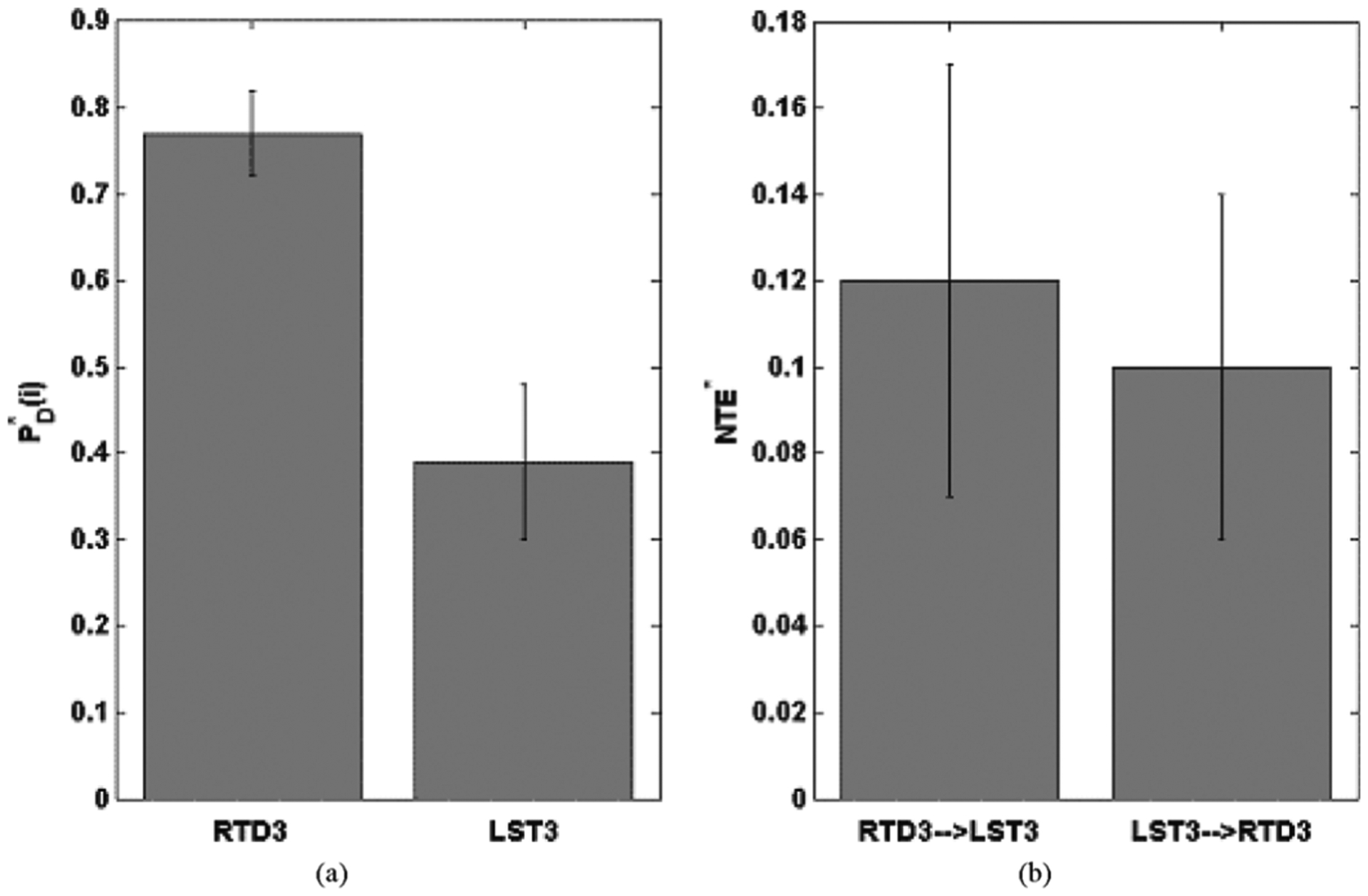
Patient 2: (a) Mean and standard deviation of intra-hemispheric at the electrode sites i determined in Step 2 as PD(i) outliers (see Fig. 3). Using the nonparametric Mann–Whitney test, the . (b) Mean and standard deviation of 23 inter-hemispheric NTE*(RTD3 → LST3) and NTE*(LST3 → RTD3). Using the nonparametric Mann–Whitney test, we find that NTE*(RTD3 → LST3) is not significantly larger than NTE*(LST3 → RTD3) (P < 0.6), implying that RTD3 and LST3 are rather “independent” foci.
In the left and right panel of Fig. 4(b), we plotted the mean and standard deviation of the 23 inter-hemispheric NTE* (RTD3 → LST3) and NTE*(LST3 → RTD3) respectively. It is observed that both and NTE*(RTD3 → LST3) and NTE* (LST3 → RTD3) are significantly larger than zero at the α = 0.05 significance level, which means that LST3 and RTD3 do interact. Even though the mean value of NTE* (RTD3 → LST3) is larger than the mean value of NTE*(LST3 → RTD3), using the nonparametric Mann–Whitney test we find that this difference is not statistically significant (P < 0.6), implying that RTD3 and LST3 appear to be “independent” foci. Therefore, Patient 2 was more probably bi-focal than uni-focal.
For completion purposes, Step 3 analysis was also performed in the other three patients. In these patients, Step 3 gives us the opportunity to rank the focal electrodes with respect to the degree of the “focality/pathology” of their dynamics, defined by the value of their . The results of this analysis have been tabulated in Table II, column 4. From this Table, it can be observed that in Patients 1, 3, and 4, the electrode that is anatomically closer to the clinically determined epileptogenic focus has the largest among all candidate focal electrodes. It thus appears that the proposed methodology may also improve the accuracy of focus localization, and hence the success of epilepsy surgery, even when applied only in interictal periods.
IV. Discussion
In this study, we suggested and implemented improvements for the estimation of TE, a measure of the direction and the level of information flow between coupled subsystems, built upon it to introduce new measures of information flow, and we showed their application to the epileptic brain. The two innovations we introduced in the TE estimation were: 1) the distance in the state space at which the required probabilities are estimated, and 2) the use of surrogate data to evaluate the statistical significance of the TE values, and then include only those values in the estimation of the average TE over time. A multivariate extension of the TE measure to detect information flow between more than two subsystems is straightforward (e.g., see [28] for such an extension of other measures).
A new measure of causality, namely net TE (NTE(i → j)), was then introduced for a system i driving a system j [see (7)]. NTE of the system i measures the outgoing net flow of information from the driving i to the driven j system. For focus localization, two more new quantities were necessary to be defined per system (brain recording site i) and for every 10.24 s of EEG data.
We called the spatial average of the statistically significant interactions NTE(i → j) over all systems j ≠ i, SANTE(i) (see Fig. 2). Thus, this quantity is specific to each electrode site i and measures the significant net information flow from i to the rest of all other electrode sites j.
We estimated the probability PD(i) of SANTE(i) being positive over an extensive period of time, that is, the percentage of time system i drives the rest of the system it significantly interacts with within a specified period of time (e.g., 6 h herein). A robust outlier detection method was then used to classify the electrode sites with respect to their PD(i)s and to identify candidate focal sites as the ones with PD(i) values greater than a suitably identified out-of-sample threshold.
Results from such an information flow-based analysis of long-term EEG data, recorded from four temporal lobe epileptic patients at two different epilepsy centers, showed a reliable localization of the epileptogenic focus in all patients. In three focal patients the focus was correctly (i.e., in agreement with the clinical assessment) localized by SANTE and PD, while in one focal patient (Patient 2) meta-processing of SANTE over time, and definition of was necessary, under the assumption that primarily focal sites drive more frequently the sites residing in their own hemisphere than the ones in the contralateral hemisphere (see Fig. 4). The location of the “major” focus correlated well with the clinical assessment (including the location of seizures’ onset and the outcome of the surgery. Existence of an additional focus was also concluded from our analysis in this patient. Interestingly, while all other three patients became seizure-free, Patient 2 continued to have seizures of reduced frequency after the operation, which gives credence to the finding from this analysis of a second, less potent but independent focus in the contralateral hemisphere.
Finally, the average probability PD of driving of the identified foci across our three uni-focal patients was 0.69. Thus, on average, the focus appeared to be driving the brain for at least 69% of the duration of the multiple-hour testing EEG data in these patients. This suggests that there are many times during the interictal period that a focus may be active. Detecting the time periods when the focus is active could help us understand the underlying mechanisms of ictogenesis (seizure generation), as well as design and implement timely interventions for seizure control [29]–[31].
V. Conclusion
In the estimation of Transfer Entropy, we introduced improvements that were shown to be critical in obtaining consistent and reliable results for driver identification. The application of this methodology to epileptogenic focus localization in four patients with focal temporal lobe epilepsy produced results in agreement with the clinical assessment of location of the focus. This is the first study to use analysis of long-term continuous EEG recordings from all available electrodes, that is, without subjective selection of EEG segments and electrodes, from different epilepsy centers and recorded with different electrode montages, to identify the epileptogenic focus/foci. Therefore, the results of the presented methodology appear to be fairly robust and may constitute the basis for the development of efficient software platforms for prospective localization of the epileptogenic focus in order to do the following.
Complement and/or replace the gold standard for focus localization currently in use in clinical practice.
Identify the extent of the focal zone.
Assist in the fast and accurate diagnosis of epilepsy by identifying single or multiple foci from interictal EEG. This could reduce the long hospitalization time currently required for focus identification, and hence reduce the economic burden for patients with epilepsy and the healthcare system.
Assist in the treatment of epilepsy by more accurately identifying the brain areas to operate upon, or to implant stimulators/drug infusion devices therein.
Acknowledgment
The authors would like to thank the anonymous reviewers for their constructive comments.
This work was supported in part by the American Epilepsy Research Foundation and the Ali Paris Fund for LKS Research and Education, in part by the National Science Foundation under Grant ECS-0601740, and in part by the Science Foundation Arizona under Competitive Advantage Award CAA 0281-08.
Biographies

Shivkumar Sabesan received the B.E. degree in electronics and telecommunications engineering from Pune University, Maharashtra, India, in 2001, and the M.S. and Ph.D. degrees in electrical engineering from Arizona State University, Tempe, in 2003 and 2008, respectively.
At present, he jointly holds a Research Scientist position in the Harrington Department of Bioengineering at Arizona State University and a Biomedical Research Engineer position at the Barrow Neurological Institute, Phoenix, AZ. His research interests are in the areas of biomedical signal processing, systems theory and nonlinear dynamics, neurophysiology, embedded systems for clinical application, clinical diagnostic monitoring, analysis and control of electrical and magnetic activity of the brain in epilepsy.

Levi B. Good received the B.S. degree in electrical engineering from the University of Wyoming, Laramie, in 1999, and the Ph.D. degree in biomedical engineering from Arizona State University, Tempe, in 2007.
He is currently a Postdoctoral Fellow in the Department of Neurology at the University of Texas Southwestern Medical Center. His research interests include biomedical signal processing, neurophysiology, brain stimulation, thalamocortical synchronization, nonlinear dynamics, control of CNS, bioinstrumentation, neuroprosthesis, and the development and testing of diagnostic and therapeutic techniques for epilepsy.

Konstantinos S. Tsakalis (M’88) received the Ph.D. degree in electrical engineering from the University of Southern California, in 1988.
He joined the Department of Electrical Engineering at Arizona State University, Tempe, in August 1988, where he is now an Associate Professor. His interests are in robust adaptive control, time varying systems, applications of control, identification, and optimization in semiconductor manufacturing problems and, more recently, the application of adaptive systems theory to the prediction and control of epileptic seizures.

Andreas Spanias (F’03) is Professor in the Department of Electrical Engineering Fulton School of Engineering at Arizona State University (ASU). He is also the Director of the SenSIP consortium. His research interests are in the areas of adaptive signal processing, speech processing, and audio sensing.
Prof. Spanias served as Associate Editor of the IEEE Transactions on Signal Processing and as General Co-chair of IEEE ICASSP-99. He also served as the IEEE Signal Processing Vice-President for Conferences. He is co-recipient of the 2002 IEEE Donald G. Fink paper prize award. He served as Distinguished lecturer for the IEEE Signal Processing Society in 2004.

David M. Treiman did his undergraduate work at the University of California, Berkeley, received the M.D. degree from Stanford University School of Medicine, Stanford, CA, and then trained in internal medicine and neurology at Duke University Medical Center, Durham, NC.
He is the Newsome Chair in Epileptology, Director of the Epilepsy Center, and Vice-chair of Neurology at the Barrow Neurological Institute, Phoenix, AZ, and Professor of Neuroscience and Bioengineering at Arizona State University, Tempe. His research has been focused on mechanisms and treatment of status epilepticus, development of new drugs and novel nonpharmacological interventions for the treatment of epilepsy, and the prediction and prevention of epileptogenesis.

Leon D. Iasemidis (M’99) received the Diploma in electrical and electronics engineering from the National Technical University, Athens, Greece, in 1982, and the M.S. degree in physics and the M.S. and Ph.D. degrees in biomedical engineering, from the University of Michigan, Ann Arbor ,in 1985, 1986, and 1991, respectively.
He is an Associate Professor of Bioengineering and an Affiliate Professor of Electrical Engineering at the Arizona State University, Tempe. His general research interests are in the areas of neuroengineering, biomedical and genomic signal processing, information theory, complex systems theory and control, neurophysiology, monitoring and analysis of the electrical and magnetic activity of the brain in epilepsy and other brain dynamical disorders, deep brain stimulation and neuromodulation, neuroplasticity, rehabilitation, and neuroprosthetics.
Contributor Information
Shivkumar Sabesan, Department of Electrical Engineering, Arizona State University, Tempe, AZ 85287 USA..
Levi B. Good, Harrington Department of Bioengineering, Arizona State University, Tempe, AZ 85287 USA.
Andreas Spanias, Department of Electrical Engineering, Arizona State University, Tempe, AZ 85287 USA..
David M. Treiman, Department of Neurology and Neurosurgery, Barrow Neurological Institute, St. Joseph’s Hospital and Medical Center, Phoenix, AZ 85006 USA.
Leon D. Iasemidis, Harrington Department of Bioengineering, Arizona State University, Tempe, AZ 85287 USA..
References
- [1].Liang H, Ding M, and Bressler S, “Temporal dynamics of information flow in the cerebral cortex,” Neurocomputing, vol. 38, pp. 1429–1435, 2001. [Google Scholar]
- [2].Vastano J and Swinney H, “Information transport in spatiotemporal systems,” Phys. Rev. Lett, vol. 60, no. 18, pp. 1773–1776, 1988. [DOI] [PubMed] [Google Scholar]
- [3].Priestly M, Spectral Analysis and Time Series. New York: Academic, 1981, vol. 1,2, Univariate Series, Multivariate Series, Prediction and Control. [Google Scholar]
- [4].Schiff S, So P, Chang T, Burke R, and Sauer T, “Detecting dynamical interdependence and generalized synchrony through mutual prediction in a neural ensemble,” Phys. Rev. E, vol. 54, no. 6, pp. 6708–6724, 1996. [DOI] [PubMed] [Google Scholar]
- [5].Chen Y, Rangarajan G, Feng J, and Ding M, “Analyzing multiple nonlinear time series with extended Granger causality,” Phys. Lett. A, vol. 324, no. 1, pp. 26–35, 2004. [Google Scholar]
- [6].Wiener N, Modern Mathematics for The Engineers [Z], ser. 1 New York: McGraw-Hill, 1956. [Google Scholar]
- [7].Schreiber T, “Measuring information transfer,” Phys. Rev. Lett, vol. 85, no. 2, pp. 461–464, 2000. [DOI] [PubMed] [Google Scholar]
- [8].Sabesan S, Narayanan K, Prasad A, Spanias A, and Iasemidis L, “Improved measure of information flow in coupled nonlinear systems,” in Proc. Int. Assoc. Sci. Technol. Develop. Int. Conf, 2003, pp. 24–26. [Google Scholar]
- [9].Sabesan S, Narayanan K, Prasad A, Tsakalis K, Spanias A, and Iasemidis L, “Information flow in coupled nonlinear systems: Application to the epileptic human brain,” in Data Mining in Biomedicine, Springer Optimization and its Applications Series, Pardalos P, Boginski V, and Vazacopoulos A, Eds. New York: Springer, 2007, pp. 483–504. [Google Scholar]
- [10].Hlaváčková-Schindler K, Paluš M, Vejmelka M, and Bhattacharya J, “Causality detection based on information-theoretic approaches in time series analysis,” Phys. Rep, vol. 441, no. 1, pp. 1–46, 2007. [Google Scholar]
- [11].Pereda E, Quiroga R, and Bhattacharya J, “Nonlinear multivariate analysis of neurophysiological signals,” Progress Neurobiol, vol. 77, no. 1–2, pp. 1–37, 2005. [DOI] [PubMed] [Google Scholar]
- [12].Bharucha-Reid A, Elements of the Theory of Markov Processes and Their Applications. Mineola, NY: Courier Dover, 1997. [Google Scholar]
- [13].Quiroga R, Arnhold J, Lehnertz K, and Grassberger P, “Kulback-Leibler and renormalized entropies: Applications to electroencephalograms of epilepsy patients,” Phys. Rev. E, vol. 62, no. 6, pp. 8380–8386, 2000. [DOI] [PubMed] [Google Scholar]
- [14].Paluš M, Komárek V, Hrnčíř Z, and těrbová K, “Synchronization as adjustment of information rates: Detection from bivariate time series,” Phys. Rev. E, vol. 63, no. 4, p. 46211, 2001. [DOI] [PubMed] [Google Scholar]
- [15].Katz R, “Criteria for estimating the order of a Markov chain,” Techno-metrics, vol. 23, no. 3, pp. 243–250, 1981. [Google Scholar]
- [16].Martinerie J, Albano A, Mees A, and Rapp P, “Mutual information, strange attractors, and the optimal estimation of dimension,” Phys. Rev. A, vol. 45, no. 10, pp. 7058–7064, 1992. [DOI] [PubMed] [Google Scholar]
- [17].Pawelzik K and Schuster H, “Generalized dimensions and entropies from a measured time series,” Phys. Rev. A, vol. 35, no. 1, pp. 481–484, 1987. [DOI] [PubMed] [Google Scholar]
- [18].Theiler J, “Spurious dimension from correlation algorithms applied to limited time-series data,” Physical Review A, vol. 34, no. 3, pp. 2427–2432, 1986. [DOI] [PubMed] [Google Scholar]
- [19].Eckmann J and Ruelle D, “Ergodic theory of chaos and strange attractors,” in Turbulence, Strange Attractors, and Chaos. Singapore: World Scientific, 1995. [Google Scholar]
- [20].Iasemidis L, Sackellares J, and Savit R, “Quantification of hidden time dependencies in the EEG within the framework of nonlinear dynamics,” Nonlinear Dynamical Anal. EEG, pp. 30–47, 1993. [Google Scholar]
- [21].Grassberger P, “Finite sample corrections to entropy and dimension estimates,” Physics Letters A, vol. 128, no. 6–7, pp. 369–373, 1988. [Google Scholar]
- [22].Engel J and Pedley T, Epilepsy: A Comprehensive Textbook. Philadelphia, PA: Lippincott-Raven, 1997. [Google Scholar]
- [23].Schwartzkroin P, “Origins of the epileptic state,” Epilepsia, vol. 38, no. 8, pp. 853–858, 1997. [DOI] [PubMed] [Google Scholar]
- [24].Engel J Jr, Van Ness P, Rasmussen T, and Ojemann L, “Outcome with respect to epileptic seizures,” Surgical Treatment Epilepsies, vol. 2, pp. 609–621, 1993. [Google Scholar]
- [25].Arnhold J, Grassberger P, Lehnertz K, and Elger C, “A robust method for detecting interdependences: Application to intracranially recorded EEG,” Physica D: Nonlinear Phenomena, vol. 134, no. 4, pp. 419–430, 1999. [Google Scholar]
- [26].Mormann F, Lehnertz K, David P, and Elger CE, “Mean phase coherence as a measure for phase synchronization and its application to the EEG of epilepsy patients,” Physica D: Nonlinear Phenomena, vol. 144, no. 3–4, pp. 358–369, 2000. [Google Scholar]
- [27].Carling K, “Resistant outlier rules and the non-Gaussian case,” Computational Statistics and Data Analysis, vol. 33, no. 3, pp. 249–258, 2000. [Google Scholar]
- [28].Friston K, “Brain function, nonlinear coupling, and neuronal transients,” Neuroscientist, vol. 7, no. 5, pp. 406–18, 2001. [DOI] [PubMed] [Google Scholar]
- [29].Iasemidis L et al. , “Epileptogenic focus localization by dynamical analysis of interictal periods of EEG in patients with temporal lobe epilepsy,” Epilepsia, vol. 38, no. Suppl 8, p. 213, 1997. [Google Scholar]
- [30].Iasemidis L, “Epileptic seizure prediction and control,” Biomedical Engineering, IEEE Transactions on, vol. 50, no. 5, pp. 549–558, 2003. [DOI] [PubMed] [Google Scholar]
- [31].Tsakalis K and Iasemidis L, “Control aspects of a theoretical model for epileptic seizures,” Int. J. Bifurcation Chaos, vol. 16, no. 7, pp. 2013–2027, 2006. [Google Scholar]