

Abstract
In order to reveal the dissolution process, the adsorption kinetics and diffusion theory are combined and used to describe the adsorption-diffusion mechanism. This can not only predict the solubility of supercritical CO2 in polymer melts but also describe two important parameters of supercritical CO2 in the dissolution process: dissolution amount and dissolution rate, which can provide a good theoretical basis for microcellular foaming. To verify the feasibility and accuracy of the theoretical calculation method, an experimental device for the volume-changing method under static condition was established. The results showed that the theoretical calculation value was in good agreement with the experimental value. In addition, the dissolution amount and dissolution rate of supercritical CO2 in three polystyrene melts with different molecular weights under different temperature and pressure conditions were measured. The results showed that the difference of polystyrene molecular weight can cause the change of dissolution rate during the dissolution process, that is, the larger the molecular weight, the slower the dissolution rate.
1. Introduction
As we know, a kind of fluid can be considered as the supercritical fluid only when its temperature and pressure are satisfied with the critical values. As one of the most important supercritical fluids, supercritical CO2 has been widely used by many people1 because of its environment friendliness, harmlessness, non-inflammability, low price, and easy control. In addition, compared with others, it also has better supercritical properties2 because its critical temperature is near the room temperature, its critical pressure is moderate, and its density is high. Supercritical CO2 has been widely used in polymer processing, such as extraction of contaminants from polymers,3 supercritical reactions,2,4 CO2-assisted polymer impregnation,5 particle preparation,6 and polymer blending.7 It turned out that the use of supercritical CO2 has attracted more and more attention8−10 in academic research and industrial applications.
The problem faced in actual research of polymer foaming is how to control the flow of CO2 and how to make CO2 dissolve more in polymer melts during the processing time.8 The above two issues need to be based on the analysis of the dissolution mechanism of CO2 in polymers. At the same time, the dissolved amount, solubility, and dissolution rate of supercritical CO2 in polymers should be accurately calculated and studied. However, there are some lacks in the solubility and dissolution data of CO2 in polymer melts for the optional design of the foaming process.
The solubility data of gases have been studied by many scholars. Hilic11 analyzed new experimental results for the solubility of nitrogen and carbon dioxide in polystyrene, accompanied by data on the change in volume of the polymer caused by the sorption process. Stao12−14 studied the solubility of CO2 in polystyrene (PS), polypropylene (PP), and high-density polyethylene (HDPE) by using the pressure decay method with the temperature up to 473.2 K and the pressure range of 2.5-20 MPa. Knez15−19 measured the solubility and diffusivity of supercritical CO2 in poly(l-lactide)-hydroxyapatite and poly(d,l-lactide-co-glycolide)-hydroxyapatite composite biomaterials by the method of magnetic suspension balance at a temperature range of 306–343 K and a pressures range of 0.1–30 MPa. Wu20 discussed the solubility and the diffusion coefficient of CO2 in PS with the gravimetric method. It turned out that the solubility increased with pressure and decreased with temperature. The diffusion coefficient of CO2 increased with the increment of the saturated time, and being a certain amount of adsorption, the diffusion coefficient decreased. Muoi21 studied the absorption and diffusion of supercritical CO2 in polycarbonate (PC) and polysulfone (PSF) melts by using a high-precision electronic balance to obtain the desorption amount by the mass loss method. In order to avoid errors caused by desorption during sample taking out, the quartz crystal microbalance method22−24 was used. In this method, the balance was placed directly under a high-pressure dissolution environment for measurement; however, the balance has a limited temperature tolerance. To overcome the temperature limitation, the magnetic suspension method was used instead in the experiment.17,25 Lashkarbolooki26 compared the capability of artificial neural network and equation of state (EOS) for the prediction of solid solubilities in supercritical CO2. Merker27 studied dissolution behavior using the molecular simulation method. Li28−31 used the neural network model to predict the solubility of supercritical CO2 in polymer melts. The existing studies in the literature focus on the solubility of CO2 in polymer melts, rather than analyzing the whole dissolution process based on the adsorption and diffusion mechanism.
The study mainly focused on three aspects. The first one is to study the dissolution characteristics of supercritical CO2+PS systems at elevated pressures and temperatures. The experiments of molten PS with a given mass under static conditions at 443.15–473.15 K and 7.5–10.5 MPa were carried out. In the experiments, the dissolved amount and dissolution rate of supercritical CO2 in different molecular weight PS under different pressures and temperatures were investigated. The second one is to reveal the change of polymer volume when the supercritical CO2 was dissolved. The experimental data were correlated using the Sanchez and Lacombe equation of state (S-L EOS), which was based on an Ising fluid model. The last and most important aspect is that the adsorption kinetics and diffusion theory were combined and used to describe the dissolution mechanism of supercritical CO2 in polymer melts under static conditions, that is, adsorption-diffusion mechanism. In addition, the dissolution amount and dissolution rate of supercritical CO2 in polymer melts were calculated, and the solubility was predicted. Then, the feasibility through experiment data was verified.
2. Results and Discussion
2.1. Dissolved Amount
In the static dissolution experiment, the amount of supercritical CO2 dissolved in the PS melt was obtained by the displacement of the piston at different times. The dissolved amount at different times can be plotted as the following curves, and the time-varying dissolved amount of supercritical CO2 in the PS melt at different pressures and temperatures can be obtained. On the other hand, through theoretical calculations based on adsorption and diffusion theories and using MATLAB to plot the calculation results, the effects of temperature and pressure on dissolution under static conditions are studied.
The dissolved amount of supercritical CO2 in PS (Mw = 1.87 × 10⁵) under different temperatures at 443.15, 453.15, 463.15, and 473.15 K are shown in Figures 1, 2, 3, and 4, respectively [(a) the time-varying dissolved amount by experiment and calculation at 7.5 MPa, (b) the time-varying dissolved amount by experiment and calculation at 8.5 MPa, (c) the time-varying dissolved amount by experiment and calculation at 9.5 MPa, and (d) the time-varying dissolved amount by experiment and calculation at 10.5 MPa].
Figure 1.

Dissolved amount of experiment and calculation at 443.15 K: (a) 7.5 MPa; (b) 8.5 MPa; (c) 9.5 MPa; (d) 10.5 MPa.
Figure 2.

Dissolved amount of experiment and calculation at 453.15 K: (a) 7.5 MPa; (b) 8.5 MPa; (c) 9.5 MPa; (d) 10.5 MPa.
Figure 3.

Dissolved amount of experiment and calculation at 463.15 K: (a) 7.5 MPa; (b) 8.5 MPa; (c) 9.5 MPa; (d) 10.5 MPa.
Figure 4.

Dissolved amount of experiment and calculation at 473.15 K: (a) 7.5 MPa; (b) 8.5 MPa; (c) 9.5 MPa; (d) 10.5 MPa.
According to the above results, some conclusions can be obtained as follows. The theoretically calculated change trend of the amount of supercritical CO2 dissolved in the polymer over time is in good agreement with the experimental result. The time-varying dissolved amount always increases until the equilibrium is reached. At a certain time, under the same temperature conditions, the higher the pressure, the greater the amount of supercritical CO2 dissolved in the polymer melt. On the contrary, when the pressure is constant, the higher the temperature, the lower the amount of supercritical CO2 dissolved in the polymer melt. Another obvious phenomenon is that, regardless of the fact that the temperature goes up or the pressure increases, the dissolution time to reach equilibrium will be shortened.
However, there are slight differences existed between the experimental results and the theoretical results. In a certain period of time, the dissolved amount of supercritical CO2 from experiment reaches a constant value, which cannot be captured by theoretical calculation. The reasons can be attributed to the following: a large amount of supercritical CO2 molecules are adsorbed on the polymer surface, which leads to a gas concentration difference between the surface and the inside of the melt, due to the concentration difference, and the CO2 molecules will continue to diffuse into the polymer melt from the surface to inside. With the dissolution continuing, the concentration difference becomes smaller and smaller, which results in the dissolution rate of supercritical CO2 in the polymer melt continuously decreasing until the dissolution equilibrium is reached. That is, the diffusion coefficient of CO2 dissolved in the polymer melt shows a downward trend over time, rather than a constant trend. However, a constant value of diffusion coefficient was used in the theoretical calculation (it can be considered an average diffusion coefficient). This will result in the phenomenon that the experimental value of the dissolved amount in the initial dissolution is slightly larger than the theoretically calculated value. The reason why the diffusion coefficient was considered to be a constant value can be attributed to the fact that the diffusion coefficients shown in the literature presented at present are all constants (average diffusion coefficient) determined through experiments under different conditions. Therefore, the constant values of diffusion coefficient was used in this article.32 In the future, we will be further studying the diffusion coefficient of supercritical CO2 in the polymer melt to understand the dissolution mechanism more comprehensively.
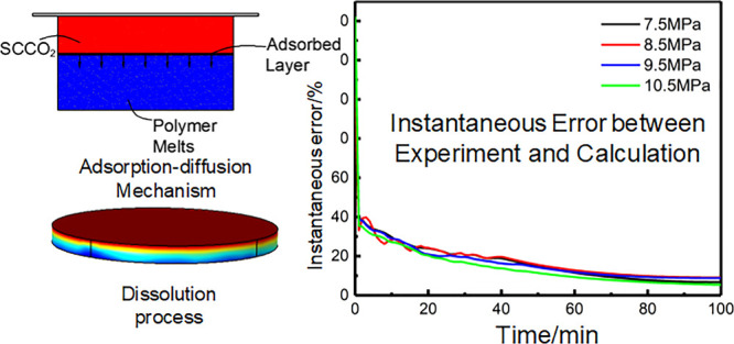
To accurately describe the comparison between the experimental values and the theoretical ones, the concept of immediate error was introduced, and the following formula was used for calculation at t moment:
| 1 |
where δt represents the instantaneous error between simulated and experimental dissolution at time t, St is a simulated value of dissolution at time t, and Sexp is an experimental value of dissolution at time t. The sampling frequency is 1 time/s, and all the discrete points are connected to obtain the instantaneous error curves of experimental and theoretical values that change with time. The instantaneous error curves are shown in Figure 5. Figures 5a, b, c, and d represent 7.5, 8.5, 9.5, and 10.5 MPa, respectively. It can be seen in the figures that the instantaneous error is decreasing over time. In the initial stage, the instantaneous errors are relatively large. As the dissolution continues, the errors between theoretical and experimental values become smaller and smaller and tend to be stable. The main reason for this phenomenon can be concluded as follows. In the early stage of the experiment, in order to ensure that the pressure in the reaction vessel reaches the preset value, the gas booster system is required to continuously inject gas, while this process is not completed instantly. The recording of the dissolution amount in the early stage will be affected by the pressurization process, and the actual dissolution amount is less than the recorded one. Therefore, the initial instantaneous errors between theoretical and experimental values are significant.
Figure 5.

Instantaneous error between theoretical and experimental dissolution: (a) 443.15 K; (b) 453.15 K; (c) 463.15 K; (d) 473.15 K.
The following data can be obtained from calculation. When the temperature is 443.15 K, the average values of the instantaneous errors under the conditions of 7.5, 8.5, 9.5, and 10.5 MPa are 14.83%, 16.68%, 18.93%, and 19.97%, respectively. When the temperature is 453.15 K, the average values of the instantaneous errors under the conditions of 7.5, 8.5, 9.5, and 10.5 MPa are 14.89%, 19.84%, 19.61%, and 17.33%, respectively. When the temperature is 463.15 K, the average values of the instantaneous errors under the conditions of 7.5, 8.5, 9.5, and 10.5 MPa are 15.88%, 17.15%, 16.74%, and 16.06%, respectively. When the temperature is 473.15 K, the average values of the instantaneous errors under the conditions of 7.5, 8.5, 9.5, and 10.5 MPa are 17.47%, 18.06%, 17.46%, and 15.05%, respectively. The calculated average instantaneous errors are below 20%. Wang et al. concluded in the literature33 that the instantaneous errors between the experiment and simulation are at about 15%. The two statements are consistent, which shows that there is a good agreement between the theoretical values and the experimental values in this article.
2.2. Solubility
A polystyrene sample of about 100 g was placed to perform the static dissolution experiments and calculations. The amount of supercritical CO2 dissolved in polymer melts shows an upward trend over time. When the dissolved amount no longer changing with time, it means that the dissolution equilibrium has been reached, at which time the dissolved amount reaches its maximum value, which is called solubility. The dissolution of supercritical CO2 will cause the expansion of the volume of the polymer melt, for which it is necessary to exclude the influence of the volume expansion of the polymer melt. In this work, the S-L EOS (Sanchez and Lacombe equation of state) based on the free volume theory was used to correlate the experimental solubility data:
| 2 |
| 3 |
p *, ρ*, and T * are the characteristic parameters of the S-L EOS, and the units of the three parameters are MPa, g·cm–3, and K, respectively. M represents the molecular weight. The S-L EOS needs to use different mixing rules when applied to the thermodynamic analysis of the binary system. The volume fraction mixing rules used in this article is as follows:13
| 4 |
| 5 |
| 6 |
| 7 |
| 8 |
| 9 |
where Ti *, pi*, ρi*, and  are the characteristic parameters of component i in the pure state. ϕ and w represent the segment fraction and mass fraction, respectively.
In the calculation of solubility, it is assumed that the dissolution
is unidirectional, that is, only the dissolution behavior of supercritical
carbon dioxide in the polymer melt occurs. It can be seen from the
S-L EOS that the solution of the equation is not unique. According
to the chemical potential of CO2 in its bulk phase equal
to its chemical potential in the polymer phase,34 the following equations can be obtained:
are the characteristic parameters of component i in the pure state. ϕ and w represent the segment fraction and mass fraction, respectively.
In the calculation of solubility, it is assumed that the dissolution
is unidirectional, that is, only the dissolution behavior of supercritical
carbon dioxide in the polymer melt occurs. It can be seen from the
S-L EOS that the solution of the equation is not unique. According
to the chemical potential of CO2 in its bulk phase equal
to its chemical potential in the polymer phase,34 the following equations can be obtained:
| 10 |
| 11 |
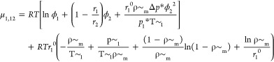 |
12 |
where, μ1,1 represents the chemical potential of CO2 in its bulk phase and μ1,12 stands for the chemical potential of CO2 in the CO2/PS mixed system. Because of the assumption that the polymer was monodisperse and did not dissolve in the gas phase, the binary interaction parameter, kij, was determined in equation 5 so as to minimize the relative deviations between experimental and calculated values at each temperature. Because kij was the factor for the energy, which would denote the interaction between two components of a system, it was correlated as a function of temperature. The form of kij is expressed as35
| 13 |
The unit of aij is K–1 and bij is dimensionless.
It can be concluded that the solubility of supercritical CO2 in polymer melts increases with increasing pressure but decreases with increasing temperature. The results in agreement with the ones in the literature.12,35,36 Although the difference between the experimental values of different molecular weights can be seen, the changes in calculated values are minimal and basically negligible. Therefore, it can be said that the difference in polymer molecular weight will not affect the solubility results. Under the same condition, comparing the solubility of the experiments and theoretical calculations, the corresponding relative error can be obtained (Table 1). This can be used as a standard to verify the accuracy of theoretical calculations. Among them, relative error 1, relative error 2, and relative error 3 respectively represent the comparison between the theoretical calculation value and the experimental value of different molecular weights (the order is Mn = 105, Mn = 1.87 × 10⁵, and Mn = 3.30 × 10⁵). The errors are maintained by about 10%, which is consistent with the literature,12−14,21,37,38 and the errors between the predicted and experimental values of solubility tend to be between 10% and 20%. As a result, the calculated results are in good agreement with the experimental ones.
Table 1. Experimental and Predicted Solubility of Supercritical CO2 in PS.
| experimental
values (g·g–1) |
||||||||
|---|---|---|---|---|---|---|---|---|
| temperature (K) | pressure (MPa) | Mw = 105 | Mw = 1.87 × 10⁵ | Mw = 3.30 × 10⁵ | theoretical values (g·g–1) | relative error 1 (%) | relative error 2 (%) | relative error 3 (%) |
| 443.15 | 7.5 | 0.02843 | 0.02785 | 0.02727 | 0.02524 | 11.221 | 9.372 | 7.444 |
| 8.5 | 0.03298 | 0.03221 | 0.03375 | 0.02946 | 10.673 | 8.538 | 12.711 | |
| 9.5 | 0.03696 | 0.03679 | 0.03662 | 0.03321 | 10.146 | 9.731 | 9.312 | |
| 10.5 | 0.04211 | 0.04147 | 0.04095 | 0.03756 | 10.805 | 9.429 | 8.278 | |
| 453.15 | 7.5 | 0.02621 | 0.02599 | 0.02577 | 0.02411 | 8.012 | 7.234 | 6.442 |
| 8.5 | 0.03081 | 0.03071 | 0.03059 | 0.02731 | 11.360 | 11.071 | 10.722 | |
| 9.5 | 0.03323 | 0.03309 | 0.03295 | 0.03051 | 8.185 | 7.797 | 7.405 | |
| 10.5 | 0.03845 | 0.03831 | 0.03791 | 0.03466 | 9.862 | 9.524 | 8.563 | |
| 463.15 | 7.5 | 0.02511 | 0.02434 | 0.02376 | 0.02307 | 8.124 | 5.218 | 2.904 |
| 8.5 | 0.02932 | 0.02921 | 0.02909 | 0.02654 | 9.482 | 9.141 | 8.766 | |
| 9.5 | 0.03123 | 0.03112 | 0.03101 | 0.02842 | 8.998 | 8.676 | 8.352 | |
| 10.5 | 0.03617 | 0.03605 | 0.03576 | 0.03210 | 11.257 | 10.965 | 10.247 | |
| 473.15 | 7.5 | 0.02408 | 0.02393 | 0.02379 | 0.02195 | 8.853 | 8.267 | 7.734 |
| 8.5 | 0.02787 | 0.02771 | 0.02759 | 0.02493 | 10.537 | 10.025 | 9.637 | |
| 9.5 | 0.03140 | 0.03122 | 0.03108 | 0.02736 | 12.862 | 12.357 | 11.968 | |
| 10.5 | 0.03266 | 0.03252 | 0.03234 | 0.02958 | 9.428 | 9.037 | 8.531 | |
2.3. Dissolution Rate
According to the dissolution curve of the dissolved amount over time, the change curve of the dissolution rate can be derived from the first-order derivation of time. In the circumstances of static dissolution, the dissolution rates of supercritical CO2 in PS with different molecular weights under different temperatures and pressures are shown in Figures 6, 7, 8, and 9, respectively [(a) the change with time of the dissolution rate of supercritical CO2 in PS with different molecular weights under 7.5 MPa, (b) the change with time of the dissolution rate of supercritical CO2 in PS with different molecular weights under 8.5 MPa, (c) the change with time of the dissolution rate of supercritical CO2 in PS with different molecular weights under 9.5 MPa, and (d) the change with time of the dissolution rate of supercritical CO2 in PS with different molecular weights under 10.5 MPa].
Figure 6.

Dissolution rate curves at 443.15 K: (a) 7.5 MPa; (b) 8.5 MPa; (c) 9.5 MPa; (d) 10.5 MPa.
Figure 7.

Dissolution rate curves at 453.15 K: (a) 7.5 MPa; (b) 8.5 MPa; (c) 9.5 MPa; (d) 10.5 MPa.
Figure 8.

Dissolution rate curves at 463.15 K: (a) 7.5 MPa; (b) 8.5 MPa; (c) 9.5 MPa; (d) 10.5 MPa.
Figure 9.

Dissolution rate curves at 473.15 K: (a) 7.5 MPa; (b) 8.5 MPa; (c) 9.5 MPa; (d) 10.5 MPa.
The rate of dissolution in the gas/polymer system depends on the diffusion rate, which helps to estimate the time required to reach equilibrium in carbon dioxide-assisted polymer processing.When the pressure is invariant, the higher the temperature, the shorter the equilibrium time, and the higher the dissolution as well. When the temperature is constant, the increase in pressure shortens the time required for supercritical CO2 to reach equilibrium in PS melts and accelerates the dissolution rate. It means that either the increase in pressure or the increase in temperature will increase the dissolution rate. This phenomenon can be explained in the following. This can be attributed to the plasticizing effect of CO2. When pressure is applied, CO2 molecules are forced into the polymer chains under the action of external forces, thereby expanding the space between the molecules and increasing the fluidity of the chains. The higher the pressure, the stronger the fluidity of the chain, and the more CO2 molecules absorbed, which explains why the increase in pressure will increase the dissolution rate.15,39 Furthermore, the movement activity of supercritical CO2 increases with the increase in temperature. As soon as dissolution occurs, the concentration of CO2 inside the PS melt is less than that of the outside, and CO2 can easily enter the polymer because of the concentration difference. The macroscopic feature is that the increase in temperature accelerates the dissolution rate, which is consistent with the literature.17,40,41 The initial dissolution rate of supercritical CO2 in PS is listed in Table 2. It can be seen that the initial dissolution rate will increase with the increase in temperature or pressure, but the change in pressure has a greater impact on the dissolution rate.
Table 2. Initial Dissolution Rate of Supercritical CO2 in PS.
| temperature (K) | pressure (MPa) | experiment 1 (g·g–1·min–1) | experiment 2 (g·g–1·min–1) | experiment 3 (g·g–1·min–1) |
|---|---|---|---|---|
| 443.15 | 7.5 | 0.00354 | 0.00313 | 0.00272 |
| 8.5 | 0.00464 | 0.00424 | 0.00336 | |
| 9.5 | 0.00647 | 0.00474 | 0.00362 | |
| 10.5 | 0.00835 | 0.00678 | 0.00472 | |
| 453.15 | 7.5 | 0.00388 | 0.00335 | 0.00301 |
| 8.5 | 0.00513 | 0.00462 | 0.00425 | |
| 9.5 | 0.00725 | 0.00605 | 0.00453 | |
| 10.5 | 0.00892 | 0.00737 | 0.00542 | |
| 463.15 | 7.5 | 0.00422 | 0.00361 | 0.00327 |
| 8.5 | 0.00588 | 0.00517 | 0.00503 | |
| 9.5 | 0.00783 | 0.00636 | 0.00486 | |
| 10.5 | 0.01081 | 0.00827 | 0.00583 | |
| 473.15 | 7.5 | 0.00502 | 0.00416 | 0.00385 |
| 8.5 | 0.00694 | 0.00601 | 0.00538 | |
| 9.5 | 0.00937 | 0.00806 | 0.00657 | |
| 10.5 | 0.01189 | 0.00949 | 0.00705 |
Meanwhile, the influence of molecular weight on dissolution was studied experimentally, as shown in Figures 6, 7, 8, and 9. By comparing the dissolution rate in PS as shown in the figures, it can be found that, under the same temperature and CO2 pressure, the CO2 dissolution rate in PS with low molecular weight is greater than that in PS with high molecular weight. That is, the dissolution rate of supercritical CO2 decreases with the increase in PS molecular weight, which is also consistent with the literature.42 This phenomenon is also visually expressed in the initial dissolution rate. The influence of the factor on dissolution rate could be explained as follows. First, the diffusion of gas in the polymer occurs mainly through its jump between free volume potentials, and the dissolution rate of gas is also closely related to the free volume. The free volume of PS with low molecular weight is larger than that of PS with high molecular weight, so the dissolution rate of CO2 in PS1 (Mn = 105) is fast. On the other hand, the complex network structure formed by the winding chains and crystalline regions formed during the dissolution process will hinder the diffusion of CO2.43 Due to the wide molecular weight distribution of PS3 (Mn = 3.30 × 10⁵), its molecular chains of different lengths are easy to be entangled, which limits the molecular motion, so its free volume is smaller than PS1, which is not conducive to the dissolution and diffusion of CO2 in PS3.
3. Conclusions
The dissolved amount, solubility, and dissolution rate of supercritical CO2 in the PS melt were predicted based on adsorption-diffusion. Compared with other studies, the innovation of this paper lies in that it focuses on the analysis of the dissolution process and the dissolution rate of supercritical CO2 in different molecular weights of PS that were added. By analyzing the dissolution mechanism and the corresponding theoretical calculated solution, we can better understand the dissolution process of supercritical carbon dioxide in the PS melt under static conditions. The calculated results are in good agreement with the experimental measurement results, which is proved to be the correctness of the theoretical numerical prediction method proposed in this paper. Nevertheless, there are some discrepancies between the experimental results and the calculated ones. Subsequently, the reasons of the discrepancies were analyzed theoretically. In the interest of improving the model prediction accuracy, it is essential that more accurate diffusion coefficients data should be considered and added to the coupled numerical calculation. In order to make the work more meaningful, the dynamic state should be added in the CO2 and different polymers binary system to improve the dissolution rate and dissolved amount for practice for future work.
4. Experimental Section
4.1. Materials
Polystyrene (PS, >99.7% purity, 100 g) was supplied by Taihua Polystyrene Co. Ltd. (Ningbo, China). Three samples with different molecular weights were contained, namely, sample 1 (Mn = 105), sample 2 (Mn = 1.87 × 10⁵), and sample 3 (Mn = 3.30 × 10⁵). All the characteristics of polystyrene were given by the supplier. CO2 (>99.5% purity) was obtained from Guohui Gas Co. Ltd. (Nanchang, China). All chemicals were used as received. The amount of PS is 100 g under different temperatures and pressures.
4.2. Apparatus and Method
The dissolved amount and dissolution rate of the gas (supercritical CO2) in the polymer (PS) melt were measured by using a volume-changing method with the apparatus, which is shown in Figure 10.
Figure 10.

Experimental apparatus for measuring the dissolved amount. (Photograph courtesy of Duyang Wang. Copyright 2020.)
Because CO2 needs a pressure greater than 7.38 MPa to reach the supercritical state, injecting CO2 directly into the reactor through a CO2 gas cylinder cannot meet this condition, and a gas booster system needs to be added. The principle of the gas booster system in this experiment has been shown in Figure 10. Start the air compressor to increase the output air pressure, connect the pressurized air to the gas booster pump to drive it to work, and continuously pressurize CO2 into the reaction vessel until the pressure condition is reached. The gas tank needs to be connected between the air compressor and the booster pump, the function of the gas tank is to ensure that the air supply is stable during the air compression process, filter the moisture and oil content in the air, and avoid causing interference to the experiment.
The single-screw air-cooled series air compressor (device model 0G06F, which is shown in Figure 11a) was produced by Shanghai Gairs Machinery Co., Ltd., Shanghai, China. The booster pump (device model DTT25NL, shown in Figure 11b) was supplied by Ji’nan Deke Tech Co., Ltd., Ji’nan, China. The high-pressure gas storage tank (device model 1V-/8, volume 1.0 m3, shown in Figure 11c) was produced by Dingxin Pressure Vessel Co., Ltd., Linyi, China.
Figure 11.

Principle and equipment of gas booster system: (a) air compressor; (b) booster pump; (c) gas tank. (Photograph courtesy of Duyang Wang. Copyright 2020.)
The experiment was conducted with the temperature range of 443.15–473.15 K and the pressure range f 7.5–10.5 MPa. The other details of the experimental procedures and structure diagram about the experimental system had been described elsewhere.33,44 The volume of the polymers under high temperatures and high pressures that were required to determine solubility accurately was obtained by PVT measurements. The oil bath was used to heat the reaction vessel through a lifting device, and the accuracy of temperature sensor in oil bath and the cells was ±0.1 °C. The accuracy of pressure sensor in each cell and the piston displacement sensor were ±0.01 MPa and ±0.05 mm, respectively. The displacement information of the piston was transmitted to the computer via the displacement sensor, and the frequency at which the computer collects the signal was 1 time/s.
5. Dissolution Mechanism and Governing Equation
In this paper, the dissolution mechanism of supercritical CO2 in polymer melts was proposed based on the essence of supercritical CO2 dissolution behavior and the theory of combining adsorption and diffusion. The solubility of supercritical CO2 in polystyrene was analyzed qualitatively, and the dissolution rate was quantitatively calculated according to the adsorption and diffusion mechanism.
5.1. Dissolution Mechanism
In the processing of microcellular plastics, the dissolution behavior of supercritical CO2 mainly occurs in the process of homogeneous formation,45 as shown in Figure 12. According to the formation process of dissolution, the adsorption kinetics and diffusion theory were combined and used to describe the adsorption-diffusion mechanism. It can be divided into the following three stages:
I. Independent two-phases: When the supercritical CO2 is injected into a high-pressure reactor filled with the polymer melt by a pressure device, the supercritical CO2 phase and the polymer melt phase exist as separate forms.
II. Interactive two-phases: Under the action of van der Waals force, supercritical CO2 molecules are adsorbed on the surface of the polymer melt and the balance will be achieved immediately. Then, the interfacial mass transfer happens because of concentration difference, which is the main reason. The supercritical CO2 molecules adsorbed on the surface are slowly diffused into the polymer melt by the concentration gradient, that is, the adsorption-diffusion process.
III. Two-phases equilibrium: The dissolution of supercritical CO2 in the polymer melt has reached the state of saturation, which means the molecules are no longer dissolved into the melts.
Figure 12.

Process of homogeneous formation.
5.1.1. Interfacial Adsorption Mechanism
Because of the polymer melts molecules on the surface under unsaturated state, surficial free energy is relatively large. Except that, the molecules cannot flow easily, it can be reduced only by the adsorption of supercritical CO2 instead of shrinking the surface so that the interfacial force filed tends to balance.
Large amounts of supercritical CO2 molecules will collide continuously to the two-phases interface, and it will stay for a very short time before escaping back to the gas phase. It turns out that the concentration of molecules on the surface of the two phases is larger than that in the supercritical CO2 phase. This is called the phenomenon of adsorption.
5.1.2. Interfacial Mass Transfer Mechanism
Diffusion can be described as the moving process of molecules from high concentration regions to low ones due to the concentration gradient. The diffusion direction in this model is from the surface to the bottom, as shown in Figure 13. In the end, it is shown that the concentration of molecules in the mixed system gets the state of equilibrium, and it is also the inevitable result of the second law of thermodynamics.
Figure 13.

Schematic diagram of adsorption and diffusion mechanism.
5.2. Governing Equation
5.2.1. Adsorption Equations
As the above principle shows, the total adsorbed supercritical CO2 molecules depend on the number of supercritical CO2 molecules that collide to the interface per unit time and the time at which these colliding molecules stay at the boundary surface.46 Make a hypothesis that the number of adsorbed supercritical CO2 molecules colliding in the unit time to the surface is n and the average residence time is τ, and the sum of the adsorbed molecules σ can be expressed as
| 14 |
Because of the disorder of gas molecules collisions based on kinetic theory, we can get the following relationships:
| 15 |
However, n is generally expressed in terms of the properties of more commonly used gases, that is, pressure, temperature, and molecular weight. This expresses the fact that molecules exert pressure on the surface when they collide with it. The expression is as follows:
| 16 |
| 17 |
Where N1 and u̅ are the number of gas molecules per unit volume and average velocity, respectively. m represents the mass of a molecule. N is the Avogadro number of molecules per gram. V represents the volume per gram. According to Maxwell’s law and the ideal gas PVT equation:
| 18 |
| 19 |
| 20 |
| 21 |
The time of colliding molecules staying at the surface τ can also be called the adsorption time, and it depends on the temperature. Frenkel46 summed up the mathematical relationship and got the following relationship:
| 22 |
where τ0 is the vibration time of adsorbed molecules and Q represents the adsorption heat. The adsorption time is a fixed value for the particular gas and a given temperature. It is generally of the order of 10–7 for supercritical CO2 under the circumstances that the adsorption entropy of the molecules is equal, the parameters in the predictive equations are from experimental adsorption results, which are according to ref (46).
5.2.2. Diffusion Equations
Under the action of van der Waals force, large numbers of supercritical CO2 molecules are adsorbed on the surface of the polymer melt, which makes the gas concentration gradient between the surface and the interior of the polymer. That is, the concentration difference is the causes of the mass transfer of supercritical CO2 molecules. According to Fick’s first law
| 23 |
where J and dc/dx is the diffusion flux and concentration gradient, respectively, and D is the diffusion coefficient. The greater the concentration gradient, the greater the diffusion flux as well as the diffusion rate. It can be concluded that the diffusion rate is proportional to the concentration gradient. When the distance between the two planes is dx, Fick’s second law can be expressed as
| 24 |
The change rate of the concentration with time is equal to the negative value of the diffusion flux with the change of distance. The relationship between the concentration of supercritical CO2 and the diffusion depth as well as diffusion time can be calculated by solving Fick’s law:47
| 25 |
where A1 is constant.
5.3. Constraint Conditions
Some initial and boundary conditions are needed to be set as the constrains.48 Based on the theory of adsorption-diffusion, the adsorption balance can be reached in a very short time and the number of supercritical CO2 molecules adsorbed on the surface can be regarded as not changing with time. That is, the surface mass concentration is constant, which can be written as c0, where c0 is the surface concentration, which is determined by the adsorption, and it can be obtained from the number of adsorbed molecules on the unit interface described by eq 14. On the basis of initial and boundary conditions as the following equations
| 26 |
| 27 |
| 28 |
The solubility of supercritical CO2 in polymer melts, which is expressed in terms of S, can be described as the following equation:
| 29 |
where erfc(x) is Gauss error function and h is the height of the polymer in the hyperbaric chamber, as shown in Figure 13. The diffusion coefficient D can be achieved in ref (32). According to the expression of the abovementioned dissolved amount (eq 29), a trend graph of the dissolved amount S and the dissolving time t can be obtained.
5.4. Material Parameters
The h in the above formula cannot accurately reflect the height of the polymer melt in the high-pressure cell because of the expansibility of the melt. The density of the polymer will change when the temperature and pressure values change in the chamber. The relationship between pressure (p), specific volume (v), and temperature (T) is used to describe the compressibility of the polymer melt in the injection molding stage. The modified two-domain Tait PVT equation of state can be used:49
| 30 |
When the polymer is in a molten state
| 31 |
| 32 |
| 33 |
where v(T, p) is the specific volume at a specific temperature and pressure, v0(T) is the specific volume at zero pressure, and vt(T, p) is the transformation function. B(T) is the pressure-sensitive parameter of material, b1m–b4m and b5 are material constant. The above parameters can be obtained from the software material library. So, the height of the polymer melt can be described as
| 34 |
where v can be calculated by eqs 30–33, which is listed in Table 3. m1 is the mass of polymer, and d is the diameter of the hyperbaric chamber.
Table 3. Specific Volume of PS.
| 443.15
K |
453.15
K |
463.15
K |
473.15
K |
||||
|---|---|---|---|---|---|---|---|
| p (MPa) | v (cm3·g–1) | p (MPa) | v (cm3·g–1) | p (MPa) | v (cm3·g–1) | p (MPa) | v (cm3·g–1) |
| 7.5 | 1.00701 | 7.5 | 1.01275 | 7.5 | 1.01848 | 7.5 | 1.02422 |
| 8.5 | 1.00637 | 8.5 | 1.01207 | 8.5 | 1.01777 | 8.5 | 1.02347 |
| 9.5 | 1.00574 | 9.5 | 1.01141 | 9.5 | 1.01706 | 9.5 | 1.02272 |
| 10.5 | 1.00511 | 10.5 | 1.01073 | 10.5 | 1.01635 | 10.5 | 1.02197 |
The values of the characteristic parameters, p*, ρ*, and T * for CO2 have been determined by Wang et al.50 A temperature-dependent T * for CO2 was used by Wang et al. The parameters for PS were determined using the experimental PVT data. The characteristic parameters50 of the S-L EOS are listed in Table 4. Other parameters, such as density and viscosity of PS, can be obtained from the literature.33
Table 4. Characteristic Parameters for S-L EOS.
| substances | p* (MPa) | ρ* (g·cm–3) | T*(K) |
|---|---|---|---|
| carbon dioxide | 720.3 | 1.58 | 208.9 + 0.459T – 7.56 × 10⁻⁴T2 |
| polystyrene | 387 | 1.108 | 466.75 |
Acknowledgments
We would like to express our sincere thanks to the National Science Foundation of China (grant nos. 51403615 and 51863014) for financial support. This work was also supported by the Special Fund Project of graduate student innovation in Jiangxi (grant no. YC2017-B009).
Appendix
The numerical code involved in this article is as follows:

Author Contributions
# D.W. and Z.C. contributed equally to this work and should be considered co-first authors. X.H. proposed the concept of the paper. D.W. and L.W. conducted experiments. The photos in Figures 10 and 11 were taken by D.W. Z.C. and L.W. performed the theoretical computations. D.W. and Z.C. analyzed the results and wrote the paper.
The authors declare no competing financial interest.
References
- Abolhasani M.; Günther A.; Kumacheva E. Microfluidic studies of carbon dioxide. Angew. Chem., Int. Ed. 2014, 53, 7992–8002. 10.1002/anie.201403719. [DOI] [PubMed] [Google Scholar]
- Cooper A. I. Polymer synthesis and processing using supercritical carbon dioxide. J. Mater. Chem. 2000, 10, 207–234. 10.1039/a906486i. [DOI] [Google Scholar]
- Sunarso J.; Ismadji S. Decontamination of hazardous substances from solid matrices and liquids using supercritical fluids extraction: A review. J. Hazard. Mater. 2009, 161, 1–20. 10.1016/j.jhazmat.2008.03.069. [DOI] [PubMed] [Google Scholar]
- Wang Y.-M.; Wang Y.-J.; Lu X.-B. “Grafting-from” polymerization for uniformly bulk modification of pre-existing polymer materials via a supercritical-fluid route. Polymer 2008, 49, 474–480. 10.1016/j.polymer.2007.11.028. [DOI] [Google Scholar]
- Sicardi S.; Manna L.; Banchero M. Diffusion of disperse dyes in PET films during impregnation with a supercritical fluid. J. Supercrit. Fluids 2000, 17, 187–194. 10.1016/S0896-8446(99)00055-8. [DOI] [Google Scholar]
- Franceschi E.; De Cesaro A. M.; Feiten M.; Ferreira S. R. S.; Dariva C.; Kunita M. H.; Rubira A. F.; Muniz E. C.; Corazza M. L.; Oliveira J. V. Precipitation of β-carotene and PHBV and co-precipitation from SEDS technique using supercritical CO2. J. Supercrit. Fluids 2008, 47, 259–269. 10.1016/j.supflu.2008.08.002. [DOI] [Google Scholar]
- Walker T. A.; Raghavan S. R.; Royer J. R.; Smith S. D.; Wignall G. D.; Melnichenko Y.; Khan S. A.; Spontak R. J. Enhanced Miscibility of Low-Molecular-Weight Polystyrene/Polyisoprene Blends in Supercritical CO2. J. Phys. Chem. B 1999, 103, 5472–5476. 10.1021/jp990551f. [DOI] [Google Scholar]
- Davies O. R.; Lewis A. L.; Whitaker M. J.; Tai H.; Shakesheff K. M.; Howdle S. M. Applications of supercritical CO2 in the fabrication of polymer systems for drug delivery and tissue engineering. Adv. Drug Delivery Rev. 2008, 60, 373–387. 10.1016/j.addr.2006.12.001. [DOI] [PubMed] [Google Scholar]
- Ma Z.; Zhang G.; Yang Q.; Shi X.; Shi A. Fabrication of microcellular polycarbonate foams with unimodal or bimodal cell-size distributions using supercritical carbon dioxide as a blowing agent. J. Cell. Plast. 2013, 50, 55–79. 10.1177/0021955X13503849. [DOI] [Google Scholar]
- Ito S.; Matsunaga K.; Tajima M.; Yoshida Y. Generation of microcellular polyurethane with supercritical carbon dioxide. J. Appl. Polym. Sci. 2007, 106, 3581–3586. 10.1002/app.26854. [DOI] [Google Scholar]
- Hilic S.; Boyer S. A. E.; Pádua A. A. H.; Grolier J.-P. E. Simultaneous measurement of the solubility of nitrogen and carbon dioxide in polystyrene and of the associated polymer swelling. J. Polym. Sci., Part B: Polym. Phys. 2001, 39, 2063–2070. 10.1002/polb.1181. [DOI] [Google Scholar]
- Sato Y.; Yurugi M.; Fujiwara K.; Takishima S.; Masuoka H. Solubilities of carbon dioxide and nitrogen in polystyrene under high temperature and pressure. Fluid Phase Equilib. 1996, 125, 129–138. 10.1016/S0378-3812(96)03094-4. [DOI] [Google Scholar]
- Sato Y.; Fujiwara K.; Takikawa T.; Sumarno; Takishima S.; Masuoka H. Solubilities and diffusion coefficients of carbon dioxide and nitrogen in polypropylene, high-density polyethylene, and polystyrene under high pressures and temperatures. Fluid Phase Equilib. 1999, 162, 261–276. 10.1016/S0378-3812(99)00217-4. [DOI] [Google Scholar]
- Sato Y.; Takikawa T.; Sorakubo A.; Takishima S.; Masuoka H.; Imaizumi M. Solubility and diffusion coefficient of carbon dioxide in biodegradable polymers. Ind. Eng. Chem. Res. 2000, 39, 4813–4819. 10.1021/ie0001220. [DOI] [Google Scholar]
- Aionicesei E.; Škerget M.; Knez Ž. Measurement of CO2 solubility and diffusivity in poly(L-lactide) and poly(D,L-lactide-co-glycolide) by magnetic suspension balance. J. Supercrit. Fluids 2008, 47, 296–301. 10.1016/j.supflu.2008.07.011. [DOI] [Google Scholar]
- Aionicesei E.; Škerget M.; Knez Ž. Mathematical modelling of the solubility of supercritical CO2 in poly(L-lactide) and poly(D,L-lactide-co-glycolide). J. Supercrit. Fluids 2009, 50, 320–326. 10.1016/j.supflu.2009.06.002. [DOI] [Google Scholar]
- Škerget M.; Mandžuka Z.; Aionicesei E.; Knez Ž.; Ješe R.; Znoj B.; Venturini P. Solubility and diffusivity of CO2 in carboxylated polyesters. J. Supercrit. Fluids 2010, 51, 306–311. 10.1016/j.supflu.2009.10.013. [DOI] [Google Scholar]
- Markočič E.; Škerget M.; Knez Ž. Solubility and diffusivity of CO2 in poly(L-lactide)-hydroxyapatite and poly(D,L-lactide-co-glycolide)-hydroxyapatite composite biomaterials. J. Supercrit. Fluids 2011, 55, 1046–1051. 10.1016/j.supflu.2010.10.001. [DOI] [Google Scholar]
- Rodríguez-Meizoso I.; Werner O.; Quan C.; Knez Z.; Turner C. Phase-behavior of alkyl ketene dimmer (AKD) in supercritical carbon dioxide. The implications of using different solubility measurement methods. J. Supercrit. Fluids 2012, 61, 25–33. 10.1016/j.supflu.2011.09.010. [DOI] [Google Scholar]
- Wu X.; Peng Y.; Cai Y. Investigation on solubility and diffusion coefficients of supercritical CO2 in polymers. China Plast. 2005, 07, 59–63. [Google Scholar]
- Tang M.; Huang W.-H.; Chen Y.-P. Comparison of the sorption and diffusion of supercritical carbon dioxide into polycarbonate and polysulfone. J. Chin. Inst. Chem. Eng. 2007, 38, 419–424. 10.1016/j.jcice.2007.09.003. [DOI] [Google Scholar]
- Aubert J. H. Solubility of carbon dioxide in polymers by the quartz crystal microbalance technique. J. Supercrit. Fluids 1998, 11, 163–172. 10.1016/S0896-8446(97)00033-8. [DOI] [Google Scholar]
- Hussain Y.; Wu Y.-T.; Ampaw P.-J.; Grant C. S. Dissolution of polymer films in supercritical carbon dioxide using a quartz crystal microbalance. J. Supercrit. Fluids 2007, 42, 255–264. 10.1016/j.supflu.2007.03.011. [DOI] [Google Scholar]
- Pantoula M.; Panayiotou C. Sorption and swelling in glassy polymer/carbon dioxide systems: Part I. Sorption. J. Supercrit. Fluids 2006, 37, 254–262. 10.1016/j.supflu.2005.11.001. [DOI] [Google Scholar]
- Jacobs M. A.; Kemmere M. F.; Keurentjes J. T. F. Foam Processing of poly(ethylene-co-vinyl acetate) rubber using supercritical carbon dioxide. Polymer 2004, 45, 7539–7547. 10.1016/j.polymer.2004.08.061. [DOI] [Google Scholar]
- Lashkarbolooki M.; Vaferi B.; Rahimpour M. R. Comparison the capability of artificial neural network (ANN) and EOS for prediction of solid solubilities in supercritical carbon dioxide. Fluid Phase Equilib. 2011, 308, 35–43. 10.1016/j.fluid.2011.06.002. [DOI] [Google Scholar]
- Merker T.; Vrabec J.; Hasse H. Molecular simulation study on the solubility of carbon dioxide in mixtures of cyclohexane + cyclohexanone. Fluid Phase Equilib. 2012, 315, 77–83. 10.1016/j.fluid.2011.11.003. [DOI] [Google Scholar]
- Li M.; Huang X.; Liu H.; Liu B.; Wu Y.; Xiong A.; Dong T. Prediction of gas solubility in polymers by back propagation artificial neural network based on self-adaptive particle swarm optimization algorithm and chaos theory. Fluid Phase Equilib. 2013, 356, 11–17. 10.1016/j.fluid.2013.07.017. [DOI] [Google Scholar]
- Li M.; Huang X.; Liu H.; Liu B.; Wu Y.; Deng X. Solubility prediction of gases in polymers using fuzzy neural network based on particle swarm optimization algorithm and clustering method. J. Appl. Polym. Sci. 2013, 129, 3297–3303. 10.1002/app.39059. [DOI] [Google Scholar]
- Li M.; Huang X.; Liu H.; Liu B.; Wu Y.; Ai F. Solubility Prediction of Gases in Polymers based on Chaotic Self-adaptive Particle Swarm Optimization Artificial Neural Networks. Acta Chim. Sin. 2013, 71, 1053–1058. 10.6023/A13020193. [DOI] [Google Scholar]
- Li M.; Huang X.; Liu H.; Liu B.; Wu Y. Prediction of the gas solubility in polymers by a radial basis function neural network based on chaotic self-adaptive particle swarm optimization and a clustering method. J. Appl. Polym. Sci. 2013, 130, 3825–3832. 10.1002/app.39525. [DOI] [Google Scholar]
- Wang W. L.; Huang X. Y.; Wang D. Y.; Li M. S.; Liu H. S. A new measuring device for solubility of supercritical carbon dioxide in polymers. China Plast. 2019, 33, 97–102. [Google Scholar]
- Wang D.; Huang X.; Cai Z.; Wang W.; Wang L.; Wang S.; Li M. Experimental and simulation study on the dissolved amount and dissolution rate of supercritical CO2 in polystyrene melt. ACS Omega 2019, 4, 22464–22474. 10.1021/acsomega.9b03148. [DOI] [PMC free article] [PubMed] [Google Scholar]
- Lacombe R. H.; Sanchez I. C. Statistical thermodynamics of fluid mixtures. J. Phys. Chem. 1976, 80, 2568–2580. 10.1021/j100564a009. [DOI] [Google Scholar]
- Li D.-c.; Liu T.; Zhao L.; Yuan W.-k. Solubility and Diffusivity of Carbon Dioxide in Solid-State Isotactic Polypropylene by the Pressure-Decay Method. Ind. Eng. Chem. Res. 2009, 48, 7117–7124. 10.1021/ie8019483. [DOI] [Google Scholar]
- Zhong H.; Sun S.; Xi Z.; Liu T.; Zhao L. Solubility of CO2 in molten poly(ethylene terephthalate). CIESC J. 2013, 64, 1513–1519. [Google Scholar]
- Sato Y.; Takikawa T.; Takishima S.; Masuoka H. Solubilities and diffusion coefficients of carbon dioxide in poly (vinyl acetate) and polystyrene. J. Supercrit. Fluids 2001, 19, 187–198. 10.1016/S0896-8446(00)00092-9. [DOI] [Google Scholar]
- Boyer S. A. E.; Grolier J.-P. E. Simultaneous measurement of the concentration of a supercritical gas absorbed in a polymer and of the concomitant change in volume of the polymer. The coupled VW-PVT technique revisited. Polymer 2005, 46, 3737–3747. 10.1016/j.polymer.2005.02.068. [DOI] [Google Scholar]
- Aionicesei E.; Škerget M.; Knez Ž. Measurement and modeling of the CO2 solubility in poly(ethylene glycol) of different molecular weights. J. Chem. Eng. Data 2008, 53, 185–188. 10.1021/je700467p. [DOI] [Google Scholar]
- Kasturirangan A.; Teja A. S. Phase behavior of CO2 + biopolymer and CO2 + fluoropolymer systems. Fluid Phase Equilib. 2007, 261, 64–68. 10.1016/j.fluid.2007.07.031. [DOI] [Google Scholar]
- Nalawade S. P.; Picchioni F.; Marsman J. H.; Grijpma D. W.; Feijen J.; Janssen L. P. B. M. Intermolecular interactions between carbon dioxide and the carbonyl groups of polylactides and poly(epsilon–caprolactone). J. Controlled Release 2006, 116, e38–e40. 10.1016/j.jconrel.2006.09.038. [DOI] [PubMed] [Google Scholar]
- Hu D.; Yan L.; Liu T.; Xu Z.; Zhao L. Solubility and diffusion behavior of compressed CO2 in polyurethane oligomer. J. Appl. Polym. Sci. 2018, 136, 47100. 10.1002/app.47100. [DOI] [Google Scholar]
- Hu D.; Chen J.; Sun S.; Liu T.; Zhao L. Solubility and Diffusivity of CO2 in Isotactic Polypropylene/Nanomontmorillonite Composites in Meltand Solid States. Ind. Eng. Chem. Res. 2014, 53, 2673–2683. 10.1021/ie403580x. [DOI] [Google Scholar]
- Xingyuan H.; Duyang W.; Xiangyu D.. Experimental apparatus for dissolution behavior of supercritical CO2 in polymer melts under the interfacial renewal conditions; ZL 2016 1 0534877.8. 2018, 06 (Chinese Patent)
- Doroudiani S.; Park C. B.; Kortschot M. T. Processing and characterization of microcellular foamed high-density polyethylene/isotactic polypropylene blends. Polym. Eng. Sci. 1998, 38, 1205–1215. 10.1002/pen.10289. [DOI] [Google Scholar]
- Deboer J. H.The Dynamical Character of Adsorption; Science Press: Beijing, China,1964. pp. 4–19; Translated by Liu, Z. H.; Wang, G. T.; Yang, K. Z. [Google Scholar]
- The Diffusion of Semiconductor; Science Press: Beijing, China, 1964. pp.89, Translated by Xue, S. Y. [Google Scholar]
- Chen J.Investigation of Solubility and Diffusivity of CO2 in polypropylene Composites and Their Application in the Simulation of CO2 Foaming Injection Molding Process. Ph.D. Dissertation, East China University of Science and Technology, Shanghai, 2013. [Google Scholar]
- Liu H.; Jiang Q.; Wang D.; Lai J.; Huang X. Three-dimensional Numerical Simulation of Thin-wall Injection Molding Flow Based on Wall Slip. Polym. Mater. Sci. Eng. 2018, 34, 122–126. [Google Scholar]
- He W. N. Measurement and prediction of vapor-liquid equilibrium ratios for solutes at infinite dilution in CO2+polyvinyl acetate system at high pressures. Kagaku Kogaku Ronbunshu 1991, 17, 1138–1145. 10.1252/kakoronbunshu.17.1138. [DOI] [Google Scholar]