Experiments for in silico evaluation of Optimality of Photosynthetic Nitrogen Distribution and Partitioning in the Canopy: an Example Using Greenhouse Cucumber Plants

Abstract

Acclimation of leaf traits to fluctuating environments is a key mechanism to maximize fitness. One of the most important strategies in acclimation to changing light is to maintain efficient utilization of nitrogen in the photosynthetic apparatus by continuous modifications of between-leaf distribution along the canopy depth and within-leaf partitioning between photosynthetic functions according to local light availability. Between-leaf nitrogen distribution has been intensively studied over the last three decades, where proportional coordination between nitrogen concentration and light gradient was considered optimal in terms of maximizing canopy photosynthesis, without taking other canopy structural and physiological factors into account. We proposed a mechanistic model of protein turnover dynamics in different photosynthetic functions, which can be parameterized using leaves grown under different levels of constant light. By integrating this dynamic model into a multi-layer canopy model, constructed using data collected from a greenhouse experiment, it allowed us to test in silico the degree of optimality in photosynthetic nitrogen use for maximizing canopy carbon assimilation under given light environments.

Background

Intra-canopy nitrogen distribution in response to light has been intensively studied (Hirose and Werger, 1987; Werger and Hirose, 1991; Anten et al., 1995; Dreccer et al., 2000; Moreau et al., 2012; Hikosaka, 2016) and many studies demonstrated that, although the actual nitrogen distribution resulted in higher canopy photosynthesis than uniform nitrogen distribution, it was still suboptimal (Field, 1983; Evans, 1993; Hollinger, 1996; Hirose et al., 1997; Meir et al., 2002; Wright et al., 2006; Hikosaka, 2016). This discrepancy between optimum and reality could, on one hand, be explained by physiological limitations (Niinemets, 2012; Hikosaka, 2016). On the other hand, it might result from incorrect predictions by over-simplified models, where the effects of variations in the structural characteristics on light interception, age-dependent modifications of leaf biochemistry and photoacclimation in functional nitrogen partitioning were neglected. To incorporate these factors into the acclimation processes, a mechanistic model based on the concept of protein turnover (synthesis and degradation) was proposed to simulate the dynamics of photosynthetic nitrogen in carboxylation, electron transport and light harvesting functions along the development and ageing of the leaf (Pao et al., 2019a and 2019b). Leaf elevation angle and leaf area distribution in the canopy was measured to construct a multi-layer canopy model for simulating more realistic intra-canopy light distribution, which is used as input for the protein turnover model. By manipulating the parameters controlling nitrogen distribution and partitioning, it is possible to quantify the degree of optimality in photosynthetic nitrogen use for maximizing canopy carbon assimilation in silico.

Materials and Reagents

1. 25-L plastic boxes, as container for hydroponic system

2. Polystyrene foam boards for fixing plants onto plastic boxes

3. Rockwool cubes (10 cm × 10 cm × 6.5 cm), as growth medium in the hydroponic system (Grodan Delta; Grodan, Roermond, The Netherlands)

4. Rockwool cubes (3.6 cm × 3.6 cm × 4 cm), as seed sowing medium (Grodan A-OK Starter Plugs; Grodan, Roermond, The Netherlands)

5. Plastic plant support clips

6. N-P-K fertilizer (Ferty 2 MEGA; Planta, Regenstauf, Germany)

7. P-K fertilizer (Ferty Basisdünger 1; Planta, Regenstauf, Germany)

8. N fertilizer (YaraLiva Calcinit; Yara, Oslo, Norway)

9. Paper bags (size should be enough to contain a single cucumber lamina, which is about 15 cm × 20 cm or larger)

10. Rockwool slabs (100 cm × 20 cm × 7.5 cm), as growth medium in the greenhouse (Grodan GT Expert; Grodan, Roermond, The Netherlands)

11. Seed (Cucumis sativus ‘Aramon’, Rijk Zwaan, De Lier, The Netherlands)

12. 1% H₂SO₄ (96% H₂SO₄, Carl Roth, catalog number: 4623; preparation: 6 ml 96% H₂SO₄ mix with 1 L H₂O)

Equipment

1. Walk-in growth chambers with aeration system and controlled air temperature and humidity (Vötsch Industrietechnik, Balingen, Germany) and light source using metal halide lamps (HQI-BT 400 W/D PRO; Osram, Munich, Germany)

2. Quantum sensor LI-190R coupled with light meter LI-250A (LI-COR, Lincoln, NE, USA)

3. Light sensor logger (LI-COR, model: LI-1000, LI-1400 or LI-1500)

4. Temperature data logger (Tinytag; Gemini Data Loggers, Chichester, UK)

5. Portable photosynthesis system LI-6400XT (coupled with 6400-40 leaf chamber fluorometer) or LI-6800 (LI-COR, Lincoln, NE, USA)

6. Chlorophyll meter (Konica Minolta Sensing, model: SPAD-502)

7. Leaf area meter (LI-COR, model: LI-3100C)

8. Laboratory balance with resolution of 0.01 g (Sartorius, model: ED4202S) or with resolution of 0.1 mg for mass below 1 g (Sartorius, model: ED224S)

9. Vacuum freeze dryer (Alpha 1-4 LSC; Martin Christ Gefriertrocknungsanlagen, Osterode am Harz, Germany)

10. 3D digitizer (Fastrak; Polhemus, Colchester, USA)

Software

1. R (ver. 3.3.0 or later; R Foundation for Statistical Computing, https://www.r-project.org/); R scripts and simulated example data sets are provided to facilitate data analysis (https://github.com/yichenpao/bio-protocol/)

   1. R script 1 [data processing] (see section Data analysis A, B)

   2. R script 2 [model parameterization] (see section Data analysis C, D); required packages are ‘DEoptim’, ‘deSolve’, ‘ggplot2’, ‘reshape2’, ‘xlsx’

   3. R script 3 [simulation and in silico test] (see section Data analysis E-H); required packages are ‘DEoptim’, ‘deSolve’, ‘dplyr’, ‘ggplot2’, ‘magrittr’, ‘xlsx’

2. Digitool (customized software for 3D-digitizer, availability upon request)

Procedure

1. Raising seedlings for experiments

   1. Sow one cucumber seed (Cucumis sativus ‘Aramon’, Rijk Zwaan, De Lier, The Netherlands) in each rock-wool cube (3.6 cm × 3.6 cm × 4 cm, Figures 1A and 1B) and water sufficiently until the cubes are completely wet.

   2. Sow 20-40% more seeds (lower the germination rate and quality, more the additional amount) than the number of plants required for the experimental design in order to select for uniform seedlings in 7-10 days.

   3. Set environmental conditions to 10-15 mol m^-2 d^-1 photosynthetically active radiation (PAR) at the seedling level with 12 h light period, 24 °C day/20 °C night air temperature and 70% relative humidity.

   4. Eight days after sowing, transfer each rockwool cube into a larger rockwool cube (10 cm × 10 cm × 6.5 cm, Figure1C) and irrigate with nutrient solution of N-P-K fertilizer (0.5 g L^-1 Ferty 2 MEGA; Planta, Regenstauf, Germany; 5.7 mM N, 2.7 mM K, 0.35 mM P, 0.45 mM Mg in working solution) once every day.

2. Growth chamber experiment to parameterize the protein turnover model

   1. Transplanting and starting experiment

      1. Prepare chambers with at least three constant light intensities (one < 5, one between 10-15 and one > 25 mol photon m^-2 d^-1 PAR for cucumber) at the plant level, which should cover most variation found in the light environment during crop production.

      2. Prepare nutrient solution with at least three levels of nitrogen (one < 2.8, one 3.5-5 and one > 8.5 mM NO₃- for cucumber Aramon) using N fertilizer (YaraLiva Calcinit; Yara, Oslo, Norway) and P-K fertilizer (Ferty Basisdünger 1; Planta, Regenstauf, Germany; 5.2 mM K, 1.3 mM P, 0.82 mM Mg in working solution) if the effect of nitrogen is of interest.

      3. Transplant the seedlings when their second true leaves reach a length of 3 cm (ca. eight days grown in the larger rockwool cubes) into hydroponic system (Figure 1D), consisting of a 25-L plastic box and a piece of polystyrene foam board that fixes a rockwool cube containing a plant.

      4. Fill 25-L boxes with nutrient solution and supply the solution with air from aeration system (Figure 1E).

      5. Prepare polystyrene foam boards for supporting the plants in the hydroponic system.

         1. Cut polystyrene foam boards to make them fit onto 25-L boxes.

         2. Cut a squared opening (9.5 cm × 9.5 cm) in the middle of the boards.

         3. Fix the plants into the openings in polystyrene foam boards and position them into the 25-L boxes.

      6. Select the healthy and unshaded leaves within leaf ranks four to eight (counted acropetally) as sampled leaves in each plant and record their dates of appearance.

      7. Record light condition at the level of the sampled leaves using quantum sensor LI-190R and light meter LI-250A (LI-COR, Lincoln, NE, USA).

   2. Plant care and monitoring environmental conditions

      1. Prepare custom-made leaf holders.

         1. Make leaf holders using plastic coated metal wires to form a loop structure, consisting of a circular part which supports the leaf and a stick part which can be fixed to the stem and petiole (Figure 1F).

         2. Combine each holder with two plastic plant support clips at the stick part.

         3. Prepare leaf holders in different sizes and lengths in order to support leaves at various developmental stages.

      2. Allow plants to establish vegetative growth by removing flowers below the seventh node.

      3. Keep plants to single stem by cutting all side shoots and train the rest of the shoot above the sampled leaves downward to avoid mutual shading (Figure 1G).

      4. Renew the nutrient solution completely and record the nitrogen level in the nutrient solution once a week, fill the solution once between two times of solution renewal, and adjust pH value to 6.0-6.5 by 1% H₂SO₄ twice a week.

      5. Place data loggers Tinytag (Gemini Data Loggers, Chichester, UK) around the sampled leaves and record daily mean air temperature (T_mean, °C).

      6. Measure and record the PAR at the center of the sampled leaves (Figure 1a in Wiechers et al., 2011) weekly and adjust the angle of the leaves using leaf holders (Figure 1F) to make sure they are horizontally and fully exposed to the light, not shaded by other leaves, in order to achieve target PAR level at the leaves.

   3. Collecting data of the sampled leaves

      1. Gas exchange

         1. Conduct measurements for each environmental condition at an interval of three to four days, starting with the youngest leaves (ca. three days after leaf appearance) and then the older ones to obtain data from leaves with a wide range of ages (ca. 40-550 °Cd).

         2. Estimate age (t, °Cd) of individual leaves days from the day of its appearance to the day of measurement using daily mean temperature and a base temperature (T_base, 10 °C for cucumber):

            $$t=\sum _{\mathrm{d}\mathrm{a}\mathrm{y}\mathrm{ }\mathrm{o}\mathrm{f}\mathrm{ }\mathrm{a}\mathrm{p}\mathrm{p}\mathrm{e}\mathrm{a}\mathrm{r}\mathrm{a}\mathrm{n}\mathrm{c}\mathrm{e}}^{\mathrm{d}\mathrm{a}\mathrm{y}\mathrm{ }\mathrm{o}\mathrm{f}\mathrm{ }\mathrm{m}\mathrm{e}\mathrm{a}\mathrm{s}\mathrm{u}\mathrm{r}\mathrm{e}\mathrm{m}\mathrm{e}\mathrm{n}\mathrm{t}} \left(T_{\mathrm{m}\mathrm{e}\mathrm{a}\mathrm{n}}-T_{\mathrm{b}\mathrm{a}\mathrm{s}\mathrm{e}}\right)$$ (G1)

         3. Measure net photosynthesis rate (A_n, μmol CO₂ m^-2 s^-1, Table 1), intercellular CO₂ concentration (C_i, µmol mol^-1), photosynthetic photon flux density (PPFD, µmol m^-2 s^-1) and quantum efficiency of photosystem II electron transport (ϕ_PSII) using a portable photosynthesis system LI-6400XT or LI-6800 (LI-COR, Lincoln, NE, USA).

         4. Collect data to a .csv file (Figure 2 and Table 2), which will be used in the data analysis sections A and B for data processing (in this example ‘example_chamber_gas_exchange_data.csv’).

         5. Cut the lamina directly after the measurement for further analyses.

      2. Harvest data

         1. Measure relative chlorophyll content (SPAD value) using chlorophyll meter SPAD-502 (Minolta Camera, Japan) and leaf area by area meter LI-3100C (LI-COR, Lincoln, NE, USA) of the harvested lamina.

         2. Keep each lamina in individual paper bag and freeze them under -20 °C for storage.

         3. Precool sample shelves in the vacuum freeze dryer (Alpha 1-4 LSC; Martin Christ Gefriertrocknungsanlagen GmbH, Osterode am Harz, Germany) to 10 °C and the ice condenser to -50 °C. Freeze dry lamina samples for 48 h under pressure of 1.030 mbar and then measure the mass of freeze-dried lamina. Please note that most samples can be dried to 1-5% residual moisture; therefore, the measured dry mass should be corrected to exclude the weight of residual moisture.

         4. Grind the lamina into fine powder and analyze total nitrogen (e.g., Nelson and Sommers, 1980) and chlorophyll (e.g., Lichtenthaler, 1987) content.

         5. Collect data to a .csv file (Figure 3 and Table 3; in this example ‘example_chamber_harvest_data.csv’), which will be used in data analysis sections A and B for data processing.

      3. Quantify the empirical relationship between SPAD value and leaf chlorophyll concentration per area to facilitate non-destructive estimation in the greenhouse experiment, using a linear (Chl = a + b × SPAD) or power (Chl = a × SPAD^b) function.

3. Gas exchange measurement using portable photosynthesis system LI-6400XT or LI-6800 (LI-COR, Lincoln, NE, USA)

   1. Allow leaves to adapt for 10-20 min under measurement conditions of:

      1. Photosynthetic photon flux density (PPFD) 1,300 µmol m^-2 s^-1,

      2. Sample CO₂ 400 µmol mol^-1,

      3. Leaf temperature 25 °C,

      4. Relative humidity 55-65%,

      until Rubisco is fully activated and photosynthesis rate, stomatal conductance and fluorescence (F’) equilibrate to steady states, then read light-saturated net photosynthesis rate (A_sat, μmol CO₂ m^-2 s^-1).

   2. Measure maximum chlorophyll fluorescence (F_m’) using the multiphase flash (MPF) approach (Loriaux et al., 2013; Moualeu-Ngangue et al., 2017):

      1. Phase 1 with constant maximum irradiance for 320 ms,

      2. Phase 2 with irradiance attenuation (30% ramp depth) over 350 ms,

      3. Phase 3 with constant maximum irradiance as in phase 1 for 200 ms.

   3. Measure light response curves of net photosynthesis rate (A_n, μmol CO₂ m^-2 s^-1) under PPFD 900, 500, 250, 150, 100, 85, 70, 60, 50, 40, 0 µmol m^-2 s^-1.

   4. Total duration of this measurement is 30-40 min per leaf; notice that for old leaves or leaves grown under low light, the time of adaptation is generally longer than for young and high light-grown leaves.

   5. Quantum efficiency of photosystem II electron transport (ϕ_PSII) is computed using fluorescence data (Murchie and Lawson, 2013):

      $${\varphi }_{\mathrm{P}\mathrm{S}\mathrm{I}\mathrm{I}}=\left(F_{\mathrm{m}}^{\mathrm{\text{'}}}-F\text{'}\right)/F_{\mathrm{m}}\text{'}$$ (P1)

4. Greenhouse experiment to obtain canopy structural information and data to evaluate the protein turnover model

   1. Transplanting and starting experiment

      1. Record daily mean air temperature (T_mean, °C) near the seedlings using data logger Tinytag and transplant the seedlings when their third true leaves reach a length of 3 cm (ca. two weeks grown in the larger rockwool cubes).

      2. Transfer two plants onto one rockwool slab (100 cm × 20 cm × 7.5 cm) with a distance of 50 cm between them and 150 cm between rows (density of 1.33 plants m^-2 in a greenhouse with 96 m² of cultivation area).

      3. Supply plants with nutrient solution by drip irrigation system with nitrogen levels of interest.

   2. Plant care and monitoring environmental conditions

      1. Train the plants vertically onto wires and remove all side shoots as well as flowers below the seventh node.

      2. Record daily mean air temperature using data logger Tinytag in the greenhouse and daily integral of PAR above the canopies using quantum sensor LI-190R and light meter LI-250A.

      3. Analyze nitrate (Navone, 1964) and ammonium (following German standard methods for the examination of water, waste water and sludge, DIN 38406-5) in the nutrient supply and nitrogen concentration remained in the rockwool slabs weekly.

      4. Collect data to a .csv file (Figure 4 and Table 4; in this example ‘example_greenhouse_environment_data.csv’), which will be used in data analysis sections E-H for simulation and in silico test.

         *ID of light and nitrogen treatments are named by users and should be identical as the treatment ID in greenhouse structural data.

   3. Collecting plant data

      1. Measure leaf number, leaf elevation angle, leaf area and leaf area index non-destructively using a 3D digitizer (Chen et al., 2014) at a weekly interval (equates to roughly 100 °Cd difference between two measurements under the greenhouse condition described above) to obtain static canopy structures at various developmental stages.

      2. Estimate age (t, °Cd) of individual leaves in the canopy.

         1. Calculate total growing degree days (GDD_canopy) from the day of transplanting into greenhouse (when leaf x appeared; in this example x = 3) to the day of measurement using Eq. G1.

         2. Divide GDD_canopy by the number of leaves appeared after transplanting (excluding the first x-1 leaves) to estimate phyllochron (°Cd per leaf, interval between appearance of successive leaves), assuming constant phyllochron during the experimental period:

            $$phyllochron={GDD}_{\mathrm{c}\mathrm{a}\mathrm{n}\mathrm{o}\mathrm{p}\mathrm{y}}/\left[total leaf number-\left(x-1\right)\right]$$ (G2)

         3. Estimate the age of leaf n using phyllochron in relation to leaf x:

            $$t_{\mathrm{l}\mathrm{e}\mathrm{a}\mathrm{f}\mathrm{ }n}={GDD}_{\mathrm{c}\mathrm{a}\mathrm{n}\mathrm{o}\mathrm{p}\mathrm{y}}-\left(n-x\right)\times phyllochron$$ (G3)

      3. Measure gas exchange and relative chlorophyll content (SPAD value, used to estimate Chl non-destructively) to evaluate the performance of the functional model of photosynthetic protein turnover in the leaf.

      4. Conduct digitization and gas exchange measurement for the same plants within 2-3 days.

      5. Collect data to a .csv file (Figure 5 and Table 5; in this example ‘example_greenhouse_structure_data.csv’), which will be used in data analysis sections E-H for simulation and in silico test.

5. Digitizing plant structure and converting coordinates into structural data

   1. Digitize the structures of at least two representative plants for each treatment using a 3D digitizer (Fastrak; Polhemus, Colchester, USA).

   2. Obtain the structural information as Cartesian coordinates in a standardized sequence of points on the individual plant organs from bottom to top of a plant (modified from Kahlen and Stützel, 2007; Wiechers et al., 2011):

      1. Digitize ‘node 0’ at the base of the stem at its insertion point to the rockwool cube.

      2. Digitize ‘node 1’ opposite to the base of petiole of the first true leaf (‘Node’ in Figure 6A).

      3. Digitize ‘axil 1’ at the insertion point of the first true leaf to the stem (‘Axil’ in Figure 6A).

      4. Digitize ‘leaf 1’ with a predefined sequence and spatial arrangement of 13 points on the lamina surface (Figure 6).

      5. Continue digitizing in the sequence of ‘node n - axil n - leaf n’ until all leaves are digitized.

      6. Neglect flowers and fruits.

   3. Convert Cartesian coordinates into structural data.

      1. Leaf area: area sum of a predefined structure of triangles (Figure 6A).

      2. Leaf elevation angle (EA, °): the angle between the orientation of the leaf tip with respect to the base of the leaf (points 1 and 2 in Figure 6B) and the horizontal plane.

   4. Quantify the empirical relationships between leaf area index (LAI), EA and leaf age (t, °Cd) to simulate the dynamics of canopy structure in the in silico experiment, for example:

      $$LAI={lai}_{\mathrm{m}\mathrm{a}\mathrm{x}}/\left\{1+exp\left[\left({lai}_{\mathrm{t}0}-t\right)/{lai}_{\mathrm{s}\mathrm{c}\mathrm{a}\mathrm{l}}\right]\right\}$$ (G4)
      $$EA=90-{es}_{\mathrm{m}\mathrm{i}\mathrm{n}}\times exp\left\{-0.5\times {\left[ln\left(t/{es}_{\mathrm{t}0}\right)/{ea}_{\mathrm{s}\mathrm{c}\mathrm{a}\mathrm{l}}\right]}^2\right\}$$ (G5)

Figure 1. Raising seedlings and setup of growth chamber experiment.

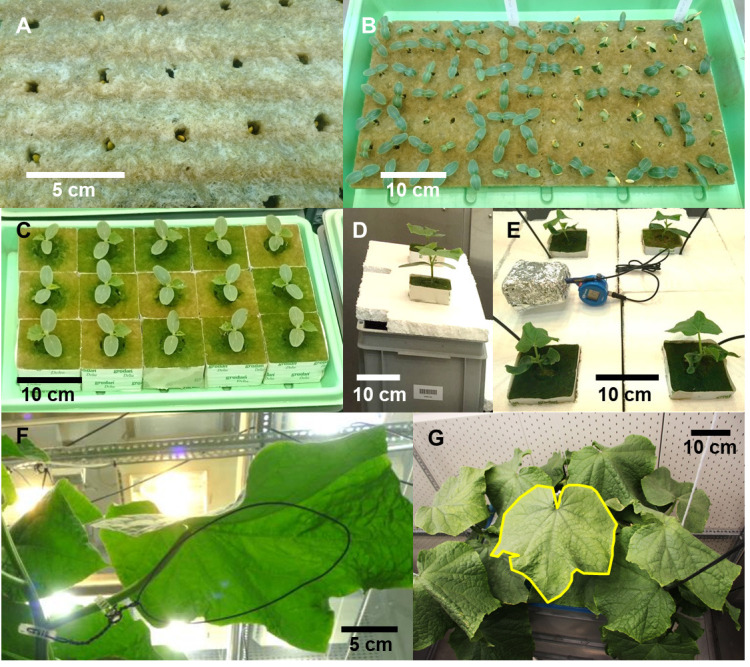
A-C. Raising seedlings in rockwool cubes. D-E. Transplanting seedlings into hydroponic system. F. Custom-made leaf holders fixed to a plant on its stem and petiole with support clips. G. Avoiding shading of the sampled leaf (marked yellow) by training rest of the shoot downward.

Table 1. Labeling of variables in the output file from portable photosynthesis systems LI-6400XT and LI-6800 (LI-COR, Lincoln, NE, USA).

Necessary variables for data processing are net photosynthesis rate (A_n, μmol CO₂ m^-2 s^-1), intercellular CO₂ concentration (C_i, µmol mol^-1), photosynthetic photon flux density (PPFD, µmol m^-2 s^-1) and quantum efficiency of photosystem II electron transport (ϕ_PSII).

System	An	Ci	PPFD	ϕPSII
LI-6400XT	Photo	Ci	PARi	PhiPS2
LI-6800	Pn	Ci	Qin	PhiPS2

Figure 2. Format of gas exchange data file.

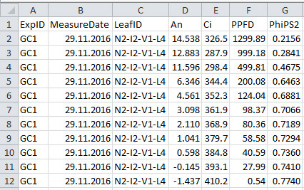
See Table 2 for explanation for column name, description and unit used.

Table 2. Column name, description and unit used in the gas exchange data file.

Column name	Description	Unit
ExpID	ID of the experiment	unitless
MeasureDate	Date of measurement	unitless
LeafID	ID of the measured leaf	unitless
An	Net photosynthesis rate	µmol CO2 m-2 s-1
Ci	intercellular CO2 concentration	µmol CO2 mol-1
PPFD	photosynthetic photon flux density	µmol photon m-2 s-1
PhiPS2	quantum efficiency of photosystem II electron transport	unitless

Figure 3. Format of harvest data file.

See Table 3 for explanation for column name, description and unit used.

Table 3. Column name, description and unit used in the harvest data file.

Column name	Description	Unit
ExpID	ID of the experiment	unitless
LeafID	ID of the harvested leaf	unitless
VarietyID	ID of the variety	unitless
LightID	ID of the light treatment	unitless
NitrogenID	ID of the nitrogen treatment	unitless
AppearanceDate	Date of appearance of the harvested leaf	unitless
HarvestDate	Date of harvest	unitless
LightLevel_mol_m2_d	Level of the light treatment	mol photon m-2 d-1
NitrogenLevel_Mm	Level of the nitrogen treatment	mM N
MeanTemp_oC	Mean air temperature during growth of the harvested leaf	°C
SPAD	Relative chlorophyll content (SPAD value)	unitless
LeafArea_cm2	Leaf area of the harvested leaf	cm2
DryMass_g	Leaf dry mass of the harvested leaf	g
TotalN_mg_g	Total nitrogen content of the harvested leaf	mg N g-1 dry mass
Chl_a_mg_g	Chlorophyll a content of the harvested leaf	mg Chl a g-1 dry mass
Chl_b_mg_g	Chlorophyll b content of the harvested leaf	mg Chl b g-1 dry mass

Figure 4. Format of greenhouse environmental data file.

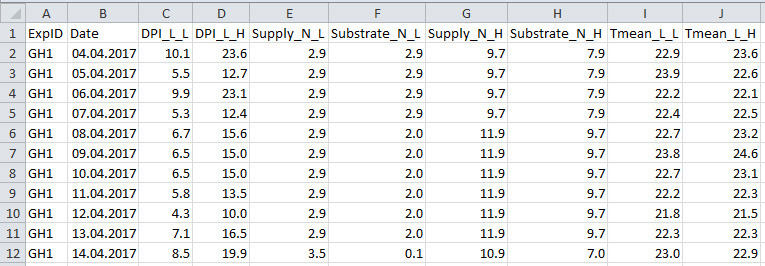
See Table 4 for explanation for column name, description and unit used.

Table 4. Column name, description and unit used in the greenhouse environmental data file.

Column name	Description	Unit
ExpID	ID of the experiment	unitless
Date	Date	unitless
DPI_L_L	Daily photon integral under light teatment ID L*	mol photon m-2 d-1
DPI_L_H	Daily photon integral under light teatment ID H*	mol photon m-2 d-1
Supply_N_L	Nitrogen level in the nutrient supply under nitrogen treatment ID L*	mM N
Substrate_N_L	Nitrogen level in the substrate under nitrogen treatment ID L*	mM N
Supply_N_H	Nitrogen level in the nutrient supply under nitrogen treatment ID H*	mM N
Substrate _N_H	Nitrogen level in the substrate under nitrogen treatment ID H*	mM N
Tmean_L_L	Daily mean air temperature under light treatment ID L*	°C
Tmean_L_H	Daily mean air temperature under light treatment ID H*	°C

Figure 5. Format of greenhouse plant structural data file.

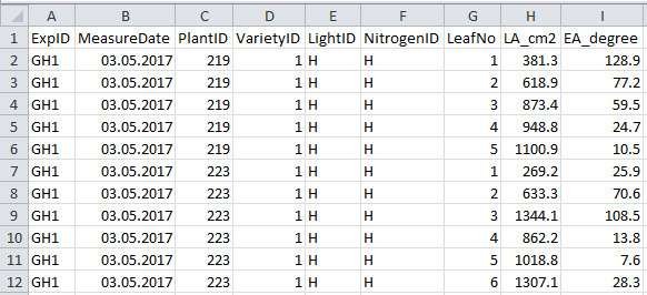
See Table 5 for explanation for column name, description and unit used.

Table 5. Column name, description and unit used in the greenhouse plant structural data file.

Column name	Description	Unit
ExpID	ID of the experiment	unitless
MeasureDate	Date of measurement	unitless
PlantID	ID of the plant digitized	unitless
VarietyID	ID of the variety digitized	unitless
LightID	ID of the light treatment	unitless
NitrogenID	ID of the nitrogen treatment	unitless
LeafNo	Rank number of the leaf digitized	unitless
EA_degree	Elevation angle of the leaf digitized
LA_cm2	Area of the leaf digitized	cm2

Figure 6. Configurations for extracting leaf area and elevation angle from digitized data.

A. Predefined positions of digitized points on the cucumber stem for a node, leaf axil, lamina and structure of triangles defined on the lamina. B. Leaf elevation angle (EA).

Data analysis

R script 1 [data processing] (Figure 7)

Figure 7. Overview of R script 1 for data processing.

Input data files for this script are ‘example_chamber_harvest_data.csv’ and ‘example_chamber_gas_exchange_data.csv’ from growth chamber experiment.

1. Estimate photosynthetic parameters using gas exchange data (Figure 7, # 1.3.0)

   1. Estimate leaf absorptance (abs, unitless) using leaf chlorophyll concentration (Chl, mmol m^-2) given by Evans (1993):

      $$abs=Chl/\left(Chl+0.076\right)$$ (P2)

   2. Estimate electron transport rate (J, μmol e- m^-2 s^-1) under various photosynthetic photon flux density (PPFD, µmol m^-2 s^-1):

      $$J=abs\times \beta \times PPFD\times {\varphi }_{\mathrm{P}\mathrm{S}\mathrm{I}\mathrm{I}}$$ (P3)

      where β (0.5, unitless) is the partitioning fraction of photons between photosystem II and I.

   3. Estimate maximum electron transport (J_max) by least squares fitting to a nonrectangular hyperbola:

      $$J=\left\{J_{\mathrm{m}\mathrm{a}\mathrm{x}}+\varphi \times PPFD-{\left[{\left(J_{\mathrm{m}\mathrm{a}\mathrm{x}}+\varphi \times PPFD\right)}^2-4\theta \times J_{\mathrm{m}\mathrm{a}\mathrm{x}}\times \varphi \times PPFD\right]}^{0.5}\right\}/\left(2\theta \right)$$ (P4)

      where ϕ (0.425 µmol e– µmol^-1 photon; Chen et al., 2014) is the conversion efficiency of photons to J, and θ (0.7, unitless; Chen et al., 2014) is a constant convexity factor describing the response of J to PPFD.

   4. Estimate daytime respiration rate (R_d, μmol CO₂ m⁻² s⁻¹) using the linear portion (40 ≤ PPFD ≤ 100 µmol m^-2 s^-1) of the light response curve (Kok, 1948) since the light compensation point in cucumber leaf is observed at ca. 40 µmol photon m^-2 s^-1.

   5. Estimate mesophyll conductance to CO₂ (g_m, mol m⁻² s⁻¹) using the variable J method (Harley et al., 1992):

      $$g_m=A_n/\left\{C_i-\left[{Г}^{*}\times \left(J+{8A}_n+{8R}_d\right)/\left(J-{4A}_n-{4R}_d\right)\right]\right\}$$ (P5)

      where Г* is CO₂ compensation point in the absence of mitochondrial respiration (43.02 µmol mol^-1 for cucumber; Singsaas et al., 2003) and C_i is intercellular CO₂ concentration (µmol mol^-1).

   6. Estimate chloroplastic CO₂ concentration (C_c, μmol mol^-1):

      $$C_{\mathrm{c}}=C_{\mathrm{i}}-A_{\mathrm{n}}/g_{\mathrm{m}}$$ (P6)

   7. Estimate maximum carboxylation rate (V_cmax, μmol CO₂ m^-2 s^-1) using the one-point method (De Kauwe et al., 2016):

      $$V_{\mathrm{c}\mathrm{m}\mathrm{a}\mathrm{x}}=\left(A_{\mathrm{s}\mathrm{a}\mathrm{t}}+R_{\mathrm{d}}\right)\times \left(C_{\mathrm{c}}+K_{\mathrm{m}}\right)/\left(C_{\mathrm{c}}-{Г}^{*}\right)$$ (P7)

      where K_m (mmol mol^-1) is given by K_c (404 μmol mol^-1) and K_o (278 mmol mol^-1), Michaelis-Menten constants of Rubisco for CO₂ and O₂, and O_c (210 mmol mol^-1) is the mole fraction of O₂ at the site of carboxylation:

      $$K_m=K_c\times \left(1+O_c/K_o\right)$$ (P8)

   8. Parameterize empirical relationships between R_d, g_m and leaf age (t, °Cd, estimated using Eq. G1), mean daily photon integral over the last four days of leaf growth (DPI_4d, mol m^-2 d^-1) and leaf photosynthetic nitrogen (N_ph, mmol m^-2) using, for example, Eq. 10 and Eqs.16 and 17 in Pao et al. (2019a):

      $$R_{\mathrm{d}}=r_{\mathrm{m}\mathrm{a}\mathrm{x}}\times {DPI}_{4\mathrm{d}}\times exp\left(-r_{\mathrm{g}}\times {DPI}_{4\mathrm{d}}\times t\right)+r_{\mathrm{m}}\times {DPI}_{4\mathrm{d}}\times t$$ (P9)
      $$g_{\mathrm{m}}=\left(g_{\mathrm{m}\mathrm{m}}\times N_{\mathrm{p}\mathrm{h}}+g_{\mathrm{m}\mathrm{m}0}\right)\times exp\left\{-0.5\times ln{\left[\left(t/g_{\mathrm{m}\mathrm{t}0}\right)/g_{\mathrm{m}\mathrm{s}\mathrm{c}\mathrm{a}\mathrm{l}}\right]}^2\right\}$$ (P10)

2. Estimate photosynthetic nitrogen pools using photosynthetic parameters (Figure 7, # 1.3.1)

   1. Estimate nitrogen involved in carboxylation (N_V, mmol N m^-2), electron transport (N_J, mmol N m^-2) and light harvesting (N_C, mmol N m^-2) following Buckley et al. (2013):

      1. N_V includes Rubisco and represents the nitrogen investment in carboxylation capacity:

         $$N_{\mathrm{V}}=V_{\mathrm{c}\mathrm{m}\mathrm{a}\mathrm{x}}/{\chi }_V$$ (M1a)

      2. N_J includes electron transport chain, photosystem II core and Calvin cycle enzymes other than Rubisco:

         $$N_{\mathrm{J}}=J_{\mathrm{m}\mathrm{a}\mathrm{x}}/{\chi }_{\mathrm{J}}$$ (M1b)

      3. N_C includes photosystem I core and light harvesting complexes I and II:

         $$N_{\mathrm{C}}=\left(Chl-N_{\mathrm{J}}\times {\chi }_{\mathrm{C}\mathrm{J}}\right)/{\chi }_{\mathrm{C}}$$ (M1c)

         where χ_V (μmol CO₂ mmol⁻¹ N s⁻¹) is the carboxylation capacity per unit Rubisco nitrogen, and χ_J (μmol e- mmol⁻¹ N s⁻¹) is the electron transport capacity per unit electron transport nitrogen. χ_CJ (mmol Chl mmol^-1 N) and χ_C (mmol Chl mmol^-1 N) are the conversion coefficients for chlorophyll per electron transport nitrogen and per light harvesting component nitrogen, respectively.

   2. Photosynthetic nitrogen (N_ph, mmol N m^-2) is defined as biologically active nitrogen in the proteins involved in photosynthetic functions, including nitrogen involved in carboxylation, electron transport and light harvesting:

      $$N_{\mathrm{p}\mathrm{h}}=N_{\mathrm{V}}+N_{\mathrm{J}}+N_{\mathrm{C}}$$ (M2)

   3. Photosynthetic nitrogen partitioning fraction of a pool X (p_X) is determined as the ratio of nitrogen in the pool X (N_X, mmol N m^-2) to N_ph:

      $$p_X=N_X/N_{\mathrm{p}\mathrm{h}}$$ (M3)

   4. Output processed data to a .csv file (Figure 8; in this example ‘chamber_processed_data.csv’) (Figure 7, # 1.4.0), which will be used in data analysis sections C and D for model parameterization.

      R script 2 [model parameterization] (Figure 9)

3. Description of protein turnover model (Figure 9, # 2.3.0)

   The rate of change of a functional nitrogen pool N_X is determined by the instantaneous protein synthesis rate (S_X(t), mmol N m^-2 °Cd^-1) and degradation rate (D_X(t), mmol N m^-2 °Cd^-1) of the corresponding enzymes and protein complexes at a given leaf age (t, °Cd):

   $$\mathrm{d}{N}_X/\mathrm{d}t=S_X\left(t\right)-D_X\left(t\right)$$ (M4)

   Protein synthesis as an age-dependent and zero-order process (Li et al., 2017), is described by a logistic function and independent of the current N_X state:

   $$S_X\left(t\right)=2S_{\mathrm{m}\mathrm{a}\mathrm{x},X}/\left[1+\mathrm{e}\mathrm{x}\mathrm{p}\left(t\times t_{\mathrm{d},X}\right)\right]$$ (M5)

   where S_max,X (mmol N m^-2 °Cd^-1) is the maximum protein synthesis rate of N_X which occurs at the early stage of leaf development. The constant t_d,X (°Cd^-1) describes the relative decreasing rate of the protein synthesis over time. At age of 1/t_d,X, S_X reduces to 53.8% of S_max,X.

   The degradation rate D_x is governed by first-order kinetics (Li et al., 2017) with a degradation constant D_r,X (°Cd^-1):

   $$D_X\left(t\right)=D_{\mathrm{r},X}\times N_X\left(t\right)$$ (M6)

   The variable S_max,X is a function of daily leaf PAR interception (DPI_{interceptLeaf}, mol photon m^-2 d^-1):

   $$S_{\mathrm{m}\mathrm{a}\mathrm{x},X}=S_{\mathrm{m}\mathrm{m},X}\times k_{\mathrm{I},X}\times {DPI}_{\mathrm{i}\mathrm{n}\mathrm{t}\mathrm{e}\mathrm{r}\mathrm{c}\mathrm{e}\mathrm{p}\mathrm{t}\mathrm{L}\mathrm{e}\mathrm{a}\mathrm{f}}/\left(S_{\mathrm{m}\mathrm{m},X}+k_{\mathrm{I},X}\times {DPI}_{\mathrm{i}\mathrm{n}\mathrm{t}\mathrm{e}\mathrm{r}\mathrm{c}\mathrm{e}\mathrm{p}\mathrm{t}\mathrm{L}\mathrm{e}\mathrm{a}\mathrm{f}}\right)r_{\mathrm{N},X}$$ (M7)

   where S_mm,X (mmol N m^-2 °Cd^-1) is potential maximum protein synthesis rate and k_I,X is rate constant describing the increase of S_max,X with light. The factor r_N,X increases with nitrogen level in the nutrient solution (N_S, mM) by a Michaelis-Menten constant, k_N,X (mM):

   $$r_{\mathrm{N},X}=N_{\mathrm{S}}/\left(k_{\mathrm{N},X}+N_{\mathrm{S}}\right)$$ (M8)

4. Parameterizing protein turnover model using data from growth chamber experiment (Figure 9)

   Solve differential Eqs. M4-M6 to obtain S_max,X, t_d,X and D_r,X in R using an algorithm programed with lsoda() function from ‘deSolve’ package and DEoptim() function from ‘DEoptim’ package, which minimizes the sums of squares of the residuals between observations and simulations (Figure 9, # 2.4.0). There are three steps to quantify the parameters in Eqs. M5-M8:

   1. Quantify t_d,X (Eq. M5) and D_r,X (Eq. M6) for each photosynthetic nitrogen pool using data of all environmental conditions, assuming D_r,X and t_d,X being species- and function-specific and not influenced by the light and nitrogen availabilities (Figure 9, # 2.4.1).

   2. Quantify S_max,X (Eq. M5) with the determined values of t_d,X, and D_r,X for each environmental condition (Figure 9, # 2.4.2).

   3. Determine S_mm,X, k_I,X (Eq. M7) and k_N,X (Eq. M8) from S_max,X by nonlinear least squares fitting using nls() function from ‘stats’ package, and the standard errors (se) and P values (pv) for the estimates are calculated as well (Figure 9, # 2.4.3).

   4. Output results (Figure 9, # 2.5.0) to a .csv file (Figure 10; in this example ‘parameterize_result_output.csv’), which will be used in data analysis sections E-H for simulation and in silico test.

      R script 3 [simulation and in silico test] (Figure 11)

5. Simulating leaf photosynthesis (Figure 11, # 3.6.0)

   In order to evaluate daily canopy carbon assimilation, net photosynthesis rate (A_n, μmol CO₂ m^-2 s^-1) of individual leaves in the canopy should be simulated. A_n is defined as the minimum of RuBP carboxylation-limited (A_c, mmol CO₂ m^-2 s^-1) and RuBP regeneration-limited (A_j, mmol CO₂ m^-2 s^-1) net photosynthesis rate (Farquhar et al., 1980). The steady-state A_c can be solved analytically with Eqs. 9b, 14 and 15, and A_j with Eqs. 9c, 14 and 15 in Pao et al. (2019a) with given values of leaf-to-air vapor pressure deficit (D, kPa), atmospheric CO₂ concentration (C_a, μmol mol^-1), photosynthetic photon flux density (PPFD, µmol m^-2 s^-1) at leaf level and photosynthetic parameters.

   1. Leaf level PPFD is simulated (Figure 11, # 3.4.1) following Beer-Lambert’s law (Monsi and Saeki, 2005) with canopy light extinction coefficient (k) and leaf area index (LAI) and adjusted by the cosine of leaf elevation angle (EA, °), which are estimated with leaf age using Eqs. G4 and G5 (Figure 11, # 3.3.0):

      $$PPFD={PPFD}_{\mathrm{a}\mathrm{b}\mathrm{o}\mathrm{v}\mathrm{e}\mathrm{C}\mathrm{a}\mathrm{n}\mathrm{o}\mathrm{p}\mathrm{y}}\times exp\left(-k\times LAI\right)\times \mathrm{c}\mathrm{o}\mathrm{s}\left(EA\right)$$ (P11)

      where diurnal PPFD above the canopy (PPFD_aboveCanopy, μmol m^-2 s^-1) at a given time (t_hour, h) during the day is calculated by a simple cosine bell function (Kimball and Bellamy, 1986) with daily PAR integral above the canopy (DPI_aboveCanopy, mol m^-2 d^-1) and day length (DL, h):

      $${PPFD}_{\mathrm{a}\mathrm{b}\mathrm{o}\mathrm{v}\mathrm{e}\mathrm{C}\mathrm{a}\mathrm{n}\mathrm{o}\mathrm{p}\mathrm{y}}={DPI}_{\mathrm{a}\mathrm{b}\mathrm{o}\mathrm{v}\mathrm{e}\mathrm{C}\mathrm{a}\mathrm{n}\mathrm{o}\mathrm{p}\mathrm{y}}\times \frac{\pi }{2DL}\times \frac{{10}^6}{3600}\times \mathrm{c}\mathrm{o}\mathrm{s}\left[\frac{\pi \times \left(t_{\mathrm{h}\mathrm{o}\mathrm{u}\mathrm{r}}-12\right)}{DL}\right]$$ (P12)

   2. Photosynthetic parameters J_max, V_cmax, abs, R_d and g_m

      1. Electron transport rate J_max under a given PPFD is calculated using Eq. P4.

      2. Carboxylation rate (V_c, μmol CO₂ m^-2 s^-1) is calculated based on the amount of activated Rubisco under a given PPFD (Qian et al., 2012):

         $$V_{\mathrm{c}}=V_{\mathrm{c}\mathrm{m}\mathrm{a}\mathrm{x}}\left\{0.31+\frac{0.69}{1+\mathrm{e}\mathrm{x}\mathrm{p}\left[-0.009\left(PPFD-500\right)\right]}\right\}$$ (P13)

      3. abs is calculated using Eq. P2.

      4. R_d and g_m are simulated using empirical relationships Eqs. P9 and P10 (Figure 11, # 3.3.1).

6. Simulating daily canopy carbon assimilation (Figure 11, # 3.6.0)

   Daily canopy carbon assimilation during daytime (DCA, mol d^-1) on day d is simulated with input data of:

   1. environmental information (from the appearance the leaf three until day d): T_mean (Eq. G1), DPI_aboveCanopy (Eq. P10), and nitrogen concentration in the supply solution and rockwool slabs;

   2. greenhouse canopy characteristics (on day d): leaf area (digitized data, Figure 7A) and leaf age (Eqs. G1-G3; Figure 11, # 3.5.1).

   Each leaf in a canopy is first simulated for its photosynthetic nitrogen pools until day d using Eqs. M4-M8 (Figure 11, # 3.7.0 and # 3.8.0) and photosynthetic parameters using Eqs. M1a-M1c. DPI_{interceptLeaf} during the growth is simulated using Eq. P11 (Figure 11, # 3.5.1). The mean value of DPI_aboveCanopy during the plant growth (from transplanting to measurement day) is used as DPI_aboveCanopy on day d to simulate DCA. Nitrogen level in the nutrient solution (N_S) is assumed to be the mean value of nitrogen concentration in the supply solution and rockwool slabs (Figure 11, # 3.4.1). In order to test the effect of incoming light condition on day d on the optimality of N_ph distribution and partitioning, DPI_aboveCanopy is multiplied by a factor ‘DPI multiplier’ assigned by users (Figure 11, # 3.7.2 and # 3.8.3).

   Leaf net photosynthesis is simulated for a time step of 0.1 h on day d, and summed up for every 0.1 h over the daytime to obtain daily leaf carbon assimilation (DLA, mol d^-1). DCA is calculated as the sum of DLA of all leaves in the canopy.

7. In silico experiment to test the optimality of nitrogen distribution in the canopy (Figure 11)

   To evaluate the effects of between-leaf distribution of N_ph on DCA, a distribution factor f_d is introduced into Eq. M5 to create variations in the rate of protein synthesis (Figure 11, # 3.7.0):

   $$S_X\left(t\right)=2S_{\mathrm{m}\mathrm{a}\mathrm{x},X}/\left[1+\mathrm{e}\mathrm{x}\mathrm{p}\left(t\times t_{\mathrm{d},X}\times f_{\mathrm{d}}\right)\right]$$ (S1)

   A control condition is defined with f_d = 1. Increasing f_d accelerates the decrease in the rate of protein synthesis and enhances acropetal N_ph reallocation, but it also reduces total N_ph in a canopy (N_canopy). To obtain the leaf photosynthetic nitrogen content (N_leaf,i, mmol N in leaf i) with comparable N_canopy, simulated N_leaf,i with f_d = n (denoted as N’_leaf,i) is adjusted proportionally to the ratio between N_canopy obtained with f_d = 1 and N_canopy obtained with f_d = n:

   $$N_{\mathrm{l}\mathrm{e}\mathrm{a}\mathrm{f},i}\left(f_{\mathrm{d}}=n\right)={N\text{'}}_{\mathrm{l}\mathrm{e}\mathrm{a}\mathrm{f},i}\left(f_{\mathrm{d}}=n\right)\times \left[N_{\mathrm{c}\mathrm{a}\mathrm{n}\mathrm{o}\mathrm{p}\mathrm{y}}\left(f_{\mathrm{d}}=1\right)/N_{\mathrm{c}\mathrm{a}\mathrm{n}\mathrm{o}\mathrm{p}\mathrm{y}}\left(f_{\mathrm{d}}=n\right)\right]$$ (S2)

   Photosynthetic nitrogen partitioning fraction of a pool X in leaf i (p_X,i) is set equal to the control value:

   $$p_{X,i}=N_{X,i}\left(f_{\mathrm{d}}=1\right)/N_{\mathrm{p}\mathrm{h},i}\left(f_{\mathrm{d}}=1\right)$$ (S3)

   These adjustments assure the same amount of N_canopy while changing the distribution pattern. The factor f_d is varied from 0.5 to 5.0 (Figure 11, # 3.7.1), which gives values of N_ph comparable to those observed in cucumber leaves (< 150 mmol N m^-2). Values of DCA produced by various f_d (Figure 11, # 3.7.2) are then compared with the control DCA (f_d = 1) under a given environmental condition and output (Figure 11, # 3.7.3) to a .xlsx file (in this example ‘Test_fd_result.xlsx’) and plotted (Figure 11, # 3.7.4 and Figure 12). Detailed results with N_ph and p_X at leaf level can be output (Figure 11, # 3.7.5) to a .xlsx file (in this example ‘Test_fd_result_detailed.xlsx’).

8. In silico experiment to test the optimality of nitrogen partitioning in the leaf (Figure 11)

   To evaluate the effects of within-leaf partitioning of N_ph on DCA, a partitioning factor f_p,X is introduced into Eq. M7 to modify maximum protein synthesis S_max,X, in order to create variations in partitioning pattern between the three photosynthetic nitrogen pools (Figure 11, # 3.8.0):

   $$S_{\mathrm{m}\mathrm{a}\mathrm{x},X}=\left[S_{\mathrm{m}\mathrm{m},X}\times f_{\mathrm{p},X}\times k_{\mathrm{I},X}\times I_{\mathrm{L}\mathrm{d}}/\left(S_{\mathrm{m}\mathrm{m},X}\times f_{\mathrm{p},\mathrm{X}}+{k_{\mathrm{I},X}\times I}_{\mathrm{L}\mathrm{d}}\right)\right]r_{\mathrm{N},X}$$ (S4)

   A control condition is defined by f_p,X = 1. An increase in f_p,X results in a higher rate of synthesis of N_X and increases the partitioning to pool X. The potential maximal protein synthesis rate for pool X (S_mm,X) is modified by a factor f_p,X, ranging from 0.2 to 2.0, to find the optimal within-leaf N_ph partitioning between functions which maximizes DCA (Figure 11, # 3.8.3). Partitioning pattern which maximizes DCA under a given environmental condition is identified as ‘optimal’ and then compared with the control DCA (f_p,X = 1), and the results are output (Figure 11, # 3.8.4) a .xlsx file (in this example ‘Test_fp_result.xlsx’) and plotted (Figure 11, # 3.8.5 and Figure 13). Detailed results with optimal N_ph partitioning at leaf level can be output (Figure 11, # 3.8.6) to a .xlsx file (in this example ‘Test_fp_result_detailed.xlsx’).

Figure 8. Format of processed data file output from R script 1.

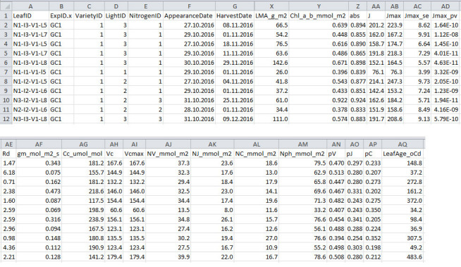
This file will be used for model parameterization.

Figure 9. Overview of R script 2 for model parameterization.

Input data file for this script is ‘chamber_processed_data.csv’ from script 1.

Figure 10. Format of parameterization result file output from R script 2.

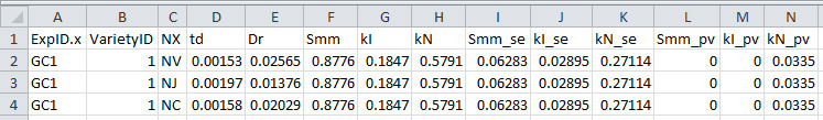
This file will be used for simulation and in silico test.

Figure 11. Overview of R script 3 for simulation and in silico test.

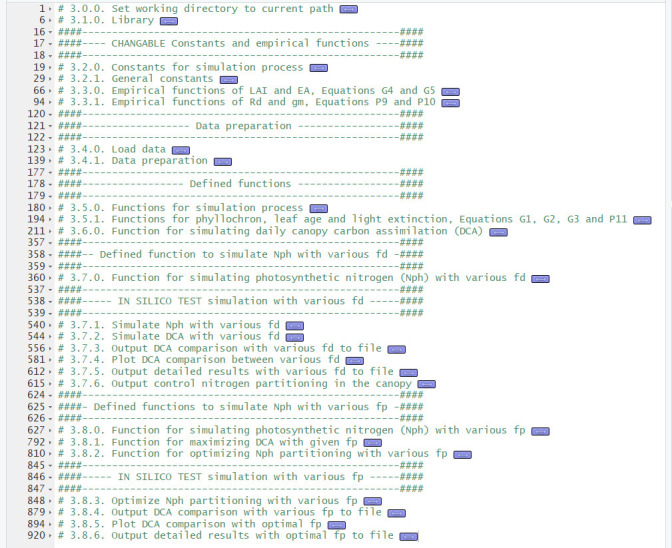
Input data files for this script are ‘example_greenhouse_structure_data.csv’ and ‘example_greenhouse_environment_data.csv’ from greenhouse experiment and ‘parameterize_result_output.csv’ from script 2.

Figure 12. Example results of percentage change in daily canopy carbon assimilation during daytime (DCA, mol d^-1) with various values of photosynthetic nitrogen (N_ph) distribution factor f_d under a given daily photosynthetically active radiation integral above the canopy (DPI, mol m^-2 d^-1).

A. DPI = mean DPI during plant growth multiplied by 0.25. B. DPI = mean DPI during plant growth. C. DPI = mean DPI during plant growth multiplied by 2. Positive change in DCA resulted from varying f_d indicates that the control N_ph distribution (f_d = 1) is sub-optimal.

Figure 13. Example results of percentage change in daily canopy carbon assimilation during daytime (DCA, mol d^-1) with various values of photosynthetic nitrogen (N_ph) partitioning factor f_p,X under mean incoming daily photosynthetically active radiation integral above the canopy (DPI, mol m^-2 d^-1) during plant growth multiplied by DPI multiplier between 0.25 and 2.0.

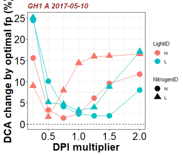
Positive change in DCA resulted from optimal f_p,X indicates that the control N_ph partitioning (f_p,X = 1) is sub-optimal. In this example, N_ph partitioning of the canopy grown under light treatment H and nitrogen treatment L is sub-optimal under its growing light environment, and DCA can be improved almost 15% if N_ph partitioning is optimized.

Competing interests

The authors declare no conflict of interest.

References

- 1.Anten N. P., Schieving F. and Werger M. J.(1995). Patterns of light and nitrogen distribution in relation to whole canopy carbon gain in C3 and C4 mono- and dicotyledonous species. Oecologia 101(4): 504-513. [DOI] [PubMed] [Google Scholar]
- 2.Buckley T. N., Cescatti A. and Farquhar G. D.(2013). What does optimization theory actually predict about crown profiles of photosynthetic capacity when models incorporate greater realism? Plant Cell Environ 36(8): 1547-1563. [DOI] [PubMed] [Google Scholar]
- 3.Chen T. W., Henke M., de Visser P. H., Buck-Sorlin G., Wiechers D., Kahlen K. and Stützel H.(2014). What is the most prominent factor limiting photosynthesis in different layers of a greenhouse cucumber canopy? Ann Bot 114(4): 677-688. [DOI] [PMC free article] [PubMed] [Google Scholar]
- 4.De Kauwe M. G., Lin Y. S., Wright I. J., Medlyn B. E., Crous K. Y., Ellsworth D. S., Maire V., Prentice I. C., Atkin O. K., Rogers A., Niinemets U., Serbin S. P., Meir P., Uddling J., Togashi H. F., Tarvainen L., Weerasinghe L. K., Evans B. J., Ishida F. Y. and Domingues T. F.(2016). A test of the'one-point method' for estimating maximum carboxylation capacity from field-measured, light-saturated photosynthesis. New Phytol 210(3): 1130-1144. [DOI] [PubMed] [Google Scholar]
- 5.Dreccer M. F., van Oijen M., Schapendonk A., Pot C. S. and Rabbinge R.(2000). Dynamics of vertical leaf nitrogen distribution in a vegetative wheat canopy. Impact on canopy photosynthesis. Ann Bot 86(4): 821-831. [Google Scholar]
- 6.Evans J. R.(1993). Photosynthetic acclimation and nitrogen partitioning within a lucerne canopy. II. Stability through time and comparison with a theoretical optimum. Functional Plant Biology 20(1): 69-82. [Google Scholar]
- 7.Farquhar G. D., von Caemmerer S. and Berry J. A.(1980). A biochemical model of photosynthetic CO2 assimilation in leaves of C3 species. Planta 149(1): 78-90. [DOI] [PubMed] [Google Scholar]
- 8.Field C.(1983). Allocating leaf nitrogen for the maximization of carbon gain: Leaf age as a control on the allocation program. Oecologia 56(2-3): 341-347. [DOI] [PubMed] [Google Scholar]
- 9.Harley P. C., Loreto F., Di Marco G. and Sharkey T. D.(1992). Theoretical considerations when estimating the Mesophyll conductance to CO2 flux by analysis of the response of photosynthesis to CO2. Plant Physiol 98(4): 1429-1436. [DOI] [PMC free article] [PubMed] [Google Scholar]
- 10.Hikosaka K.(2016). Optimality of nitrogen distribution among leaves in plant canopies. J Plant Res 129(3): 299-311. [DOI] [PubMed] [Google Scholar]
- 11.Hirose T., Ackerly D. D., Traw M. B., Ramseier D. and Bazzaz F.A.(1997). CO2 elevation, canopy photosynthesis, andoptimal leaf area index. Ecology 78(8): 2339-2350. [Google Scholar]
- 12.Hirose T. and Werger M. J.(1987). Maximizing daily canopy photosynthesis with respect to the leaf nitrogen allocation pattern in the canopy. Oecologia 72(4): 520-526. [DOI] [PubMed] [Google Scholar]
- 13.Hollinger D. Y.(1996). Optimality and nitrogen allocation in a tree canopy. Tree Physiol 16(7): 627-634. [DOI] [PubMed] [Google Scholar]
- 14.Kahlen K. and Stützel H.(2007). Estimation of geometric attributes and masses of individual cucumber organs using three-dimensional digitizing and allometric relationships. J AM SOC HORTIC SCI 132(4): 439-446. [Google Scholar]
- 15.Kimball B. A. and Bellamy L. A.(1986). Generation of diurnal solar radiation, temperature, and humidity patterns. Energy Agriculture 5(3): 185-197. [Google Scholar]
- 16.Kok B.(1948). A critical consideration of the quantum yield of Chlorella-photosynthesis. Enzymologia 13(1): 1-56. [Google Scholar]
- 17.Li L., Nelson C. J., Trösch J., Castleden I., Huang S. and Millar A. H.(2017). Protein degradation rate in Arabidopsis thaliana leaf growth and development. Plant Cell 29(2): 207-228. [DOI] [PMC free article] [PubMed] [Google Scholar]
- 18.Lichtenthaler H. K.(1987). Chlorophylls and carotenoids: pigments of photosynthetic biomembranes. Methods Enzymology 148: 350-382. [Google Scholar]
- 19.Loriaux S. D., Avenson T. J., Welles J. M., McDermitt D. K., Eckles R. D., Riensche B. and Genty B.(2013). Closing in on maximum yield of chlorophyll fluorescence using a single multiphase flash of sub-saturating intensity. Plant Cell Environ 36(10): 1755-1770. [DOI] [PubMed] [Google Scholar]
- 20.Meir P., Kruijt B., Broadmeadow M., Barbosa E., Kull O., Carswell F., Nobre A. and Jarvis P.G.(2002). Acclimation of photosynthetic capacity to irradiance in tree canopies in relation to leaf nitrogen concentration and leaf mass per unit area. Plant, Cell Environment 25(3): 343-357. [Google Scholar]
- 21.Monsi M. and Saeki T.(2005). On the factor light in plant communities and its importance for matter production. 1953. Ann Bot 95(3): 549-567. [DOI] [PMC free article] [PubMed] [Google Scholar]
- 22.Moreau D., Allard V., Gaju O., Le Gouis J., Foulkes M. J. and Martre P.(2012). Acclimation of leaf nitrogen to vertical light gradient at anthesis in wheat is a whole-plant process that scales with the size of the canopy. Plant Physiol 160(3): 1479-1490. [DOI] [PMC free article] [PubMed] [Google Scholar]
- 23.Moualeu-Ngangue D. P., Chen T. W. and Stützel H.(2017). A new method to estimate photosynthetic parameters through net assimilation rate-intercellular space CO2 concentration(A-Ci) curve and chlorophyll fluorescence measurements. New Phytol 213(3): 1543-1554. [DOI] [PubMed] [Google Scholar]
- 24.Murchie E.H. and Lawson T.(2013). Chlorophyll fluorescence analysis: a guide to good practice and understanding some new applications. J Exp Bot 64(13): 3983-3998. [DOI] [PubMed] [Google Scholar]
- 25.Navone R.(1964). Proposed method for nitrate in potable waters. Journal-American Water Works Association 56(6): 781-783. [Google Scholar]
- 26.Nelson D.W. and Sommers L.E.(1980). Total nitrogen analysis of soil and plant tissues. J Assoc Off Anal Chem 63(4):770-778. [Google Scholar]
- 27.Niinemets Ü.(2012). Optimization of foliage photosynthetic capacity in tree canopies: towards identifying missing constraints. Tree Physiol 32(5): 505-509. [DOI] [PubMed] [Google Scholar]
- 28.Pao Y. C., Chen T. W., Moualeu-Ngangue D. P. and Stützel H.(2019). Environmental triggers for photosynthetic protein turnover determine the optimal nitrogen distribution and partitioning in the canopy. J Exp Bot 70(9): 2419-2434. [DOI] [PMC free article] [PubMed] [Google Scholar]
- 29.Pao Y. C., Stutzel H. and Chen T. W.(2019). A mechanistic view of the reduction in photosynthetic protein abundance under diurnal light fluctuation. J Exp Bot 70(15): 3705-3708. [DOI] [PMC free article] [PubMed] [Google Scholar]
- 30.Qian T., Elings A., Dieleman J. A., Gort G. and Marcelis L. F. M.(2012). Estimation of photosynthesis parameters for a modified Farquhar–von Caemmerer–Berry model using simultaneous estimation method and nonlinear mixed effects model. Env Exp Bot 82: 66-73. [Google Scholar]
- 31.Singsaas E. L., Ort X. and Delucia E. H.(2003). Elevated CO2 effects on mesophyll conductance and its consequences for interpreting photosynthetic physiology. Plant, Cell Environment 27(1): 41-50. [Google Scholar]
- 32.Werger M. J. A., and Hirose T.(1991). Leaf nitrogen distribution and whole canopy photosynthetic carbon gain in herbaceous stands. Vegetatio 97(1): 11-20. [Google Scholar]
- 33.Wiechers D., Kahlen K. and Stützel H.(2011). Evaluation of a radiosity based light model for greenhouse cucumber canopies. Agr For Met 151(7): 906-915. [Google Scholar]
- 34.Wright I. J., Leishman M. R., Read C. and Westoby M.(2006). Gradients of light availability and leaf traits with leaf age and canopy position in 28 Australian shrubs and trees. Functional Plant Biology 33(5): 407-419. [DOI] [PubMed] [Google Scholar]