BAYESIAN FACTOR MODELS FOR PROBABILISTIC CAUSE OF DEATH ASSESSMENT WITH VERBAL AUTOPSIES

Abstract

The distribution of deaths by cause provides crucial information for public health planning, response and evaluation. About 60% of deaths globally are not registered or given a cause, limiting our ability to understand disease epidemiology. Verbal autopsy (VA) surveys are increasingly used in such settings to collect information on the signs, symptoms and medical history of people who have recently died. This article develops a novel Bayesian method for estimation of population distributions of deaths by cause using verbal autopsy data. The proposed approach is based on a multivariate probit model where associations among items in questionnaires are flexibly induced by latent factors. Using the Population Health Metrics Research Consortium labeled data that include both VA and medically certified causes of death, we assess performance of the proposed method. Further, we estimate important questionnaire items that are highly associated with causes of death. This framework provides insights that will simplify future data

1. Introduction.

The distribution of causes of death is an essential part of understanding population dynamics, as well as implementing and evaluating effective public health interventions (e.g., Bloomberg and Bishop (2015), Mathers et al. (2005), Ruzicka and Lopez (1990), Soleman, Chandramohan and Shibuya (2006)). Monitoring cause of death requires understanding both acute, rapid onset epidemiological crises (e.g., the outbreak of an infectious diseases) and observing changes over the course of decades (e.g., the rise in obesity related diabetes). The “gold-standard” for assigning cause of death relies on physical autopsies with pathological reports. In low-resource settings, however, most deaths happen outside of hospitals and are often not recorded by a civil registration and vital statistics systems (Mikkelsen et al. (2015)). In such settings, understanding the mortality burden of a specific cause, and trends in cause-specific mortality over time, is extremely challenging (e.g., de Savigny et al. (2017), Phillips et al. (2015)). In-person autopsies take valuable physician time away from patients to perform autopsies and are extremely difficult or impossible for deaths that happen outside of the hospital, meaning that any insights are generalizable only to the small fraction of the population that regularly interacts with the healthcare system.

Scaling up to a system that can record all deaths presents massive financial and logistical challenges, meaning that local and national governments must rely on lower cost alternatives. One common approach is to use surveys with relatives or caretakers of the decedent. There is, naturally, much less information in a survey-based system than in a physical autopsy and there are numerous data quality challenges. Nonetheless, given the lack of credible alternatives, survey-based data are and will continue to be vital for understanding cause of death distributions (AbouZahr et al. (2007), Horton (2007), Jha (2014)). Survey-based data for cause of death assessment are known as verbal autopsies (VAs) and consist of interviews with a family member or other individual familiar with the death. The respondent answers a questionnaire about the signs, symptoms, demographic characteristics and health history of the deceased individual. Deaths are typically identified using community informants or using a partial surveillance system. Interviews are conducted by specially trained enumerators, some of whom have medical expertise. VA surveys are widely conducted (Lopez (1998), Maher et al. (2010), Yang et al. (2005), Sankoh and Byass (2012)), and the World Health Organization (WHO) releases a standardized VA questionnaire to facilitate comparison across areas (World Health Organization (2012, 2017), Nichols et al. (2018)).

Given VA surveys, there are several available methods to estimate a cause of death based on the reported symptoms. In some settings, trained clinicians review VAs and assess a cause of death (Lozano et al. (2011)). This approach can be effective in some circumstances, but is time-consuming and requires that trained clinicians (many of whom would otherwise be seeing patients) be available. An alternative approach is to use an algorithmic or statistical method to assign causes of death. Several such methods have been proposed and evaluated in the statistics and public health literatures (see, e.g., Byass et al. (2012), James, Flaxman and Murray (2011), McCormick et al. (2016), Miasnikof et al. (2015), Serina et al. (2015)).

For the most part, these methods rely on a critical assumption: independence across symptoms conditional on a given cause. This assumption disregards critical information about constellations or clusters of symptoms that are typical of a given cause and thus particularly informative when assigning causes. The only method currently available that uses information about dependence between symptoms is work by King and Lu (King and Lu (2008), King, Lu and Shibuya (2010)). The King and Lu method regresses the probability of random subsets of symptoms on the conditional probability of the selected symptoms given a cause. This process is an attempt to represent the space of all possible symptom combinations. However since there are typically one to two hundred symptoms, exploring all possible combinations is an extremely daunting task, which is often impossible in reasonable time.

Our work presents a novel approach to incorporating dependence between symptoms in assigning cause of death from VA surveys. In our approach, we capture dependence between symptoms using a small number of latent factors. This approach avoids the need to evaluate all possible symptom combinations as in the King and Lu framework. We build a multivariate probit model for symptoms conditional on a cause. Binary-scale outcomes can be interpreted as a manifestation of underlying continuous variables. A factor model on these conditional variables provides a sparse covariance structure between symptoms. Our method also accommodates missing data that commonly arise in VA surveys, because for example, family members may not remember all details about sign/symptoms of the deceased person. The proposed approach can incorporate both individual-specific and design-based missing values by summing them out from the probit model with a missing-at-random assumption. We fit the model using an efficient Markov chain Monte Carlo (MCMC) algorithm we develop for posterior computation. Further, we utilize our framework to better understand the importance of each measure in the questionnaire. To do this, we quantify the association between each symptom with each cause, using a model-based version of Cramér’s V. Our measures can be used to simplify and shorten future VA surveys, decreasing both the burden on respondents and the cost.

The remainder of the paper is organized as follows. This section describes labeled VA data from the Population Health Metrics Research Consortium (PHMRC) that will be the primary data source we use in our analysis. Section 2 proposes a novel approach for estimation of population distributions of causes of death using a small number of latent factors. Section 3 develops an efficient MCMC algorithm. Section 4 assesses the performance of the proposed approach in various scenarios and measures strength of dependence of questionnaire items in the PHMRC dataset. Section 5 concludes the article.

1.1. PHMRC VA survey.

The Population Health Metrics Research Consortium (PHMRC) collected VA data at six study sites in four countries: Andhra Pradesh, India; Bohol, Philippines; Dar es Salaam, Tanzania; Mexico City, Mexico; Pemba Island, Tanzania; and Uttar Pradesh, India. In each study site, VAs were collected for adults, children and neonates in hospital and clinical environments. Causes were assigned based on diagnostic criteria including laboratory, pathology and medical imaging findings. Murray et al. (2011) provide the detailed criteria for each cause, which were developed by a committee of physicians involved in the study. The cause list was constructed based on WHO global burden of disease estimates of the leading causes of death in the developing world. VA interviews were conducted with a relative of the deceased by interviewers who were blinded to the cause of death assigned in the hospital, and the family member provided the consent for the VA study. The VA questionnaire items cover symptoms of illnesses, demographic characteristics, diagnoses of chronic illnesses by health service providers, possible risk factors such as tobacco-use and other potentially contributing characteristics. In typical settings where VA surveys are implemented, it is not possible to obtain a large fraction of deaths with physician codes. The PHMRC data are, therefore, intended to be used as training data for statistical and algorithmic methods used in settings where only VA surveys are available. Murray et al. (2011) provide detailed information of the design and implementation of the PHMRC study, approved by the University of Washington IRB. PHMRC (2013) released a version of the dataset to the public after removing potentially identifying information from the original VA interviews. The lists of causes of death and predictors in our analysis are in the Supplementary Material (Kunihama et al. (2020)).

Figure 1 shows the barplot of 34 predefined causes of death for adults in the PHMRC data, and those for each study site are in the Supplementary Material (Kunihama et al. (2020)). We observe that there is a large difference in the number of deaths between causes, for example 630 in stroke and 40 in esophageal cancer, and distributions of the causes vary considerably among the sites. The VA questionnaire consists of binary, count and categorical items. Existing statistical and algorithmic tools for assigning cause of death from VA surveys dichotomize categorical and continuous variables. We use the procedure described in Murray et al. (2011) and McCormick et al. (2016) to convert all indicators into binary variables, leading to a dataset with 7841 individuals and 175 symptoms/indicators. Dichotomizing continuous and categorical variables no doubt loses some information, but it also facilitates greater comparability with current state of the art methods for VA classification. Building models for high dimensional, mixed-scale variables remains a challenging open area of research. An additional feature of the PHMRC, and all VA data, is the presence of abundant missing values. These occur for several reasons, including difficulty recalling specific circumstances of a person’s death. Figure 2 shows the histogram of the missing rate of the binary predictors. We observe many predictors contain missing values and in some cases the missingness is extreme, with more than half of questions missing answers.

Fig. 1.

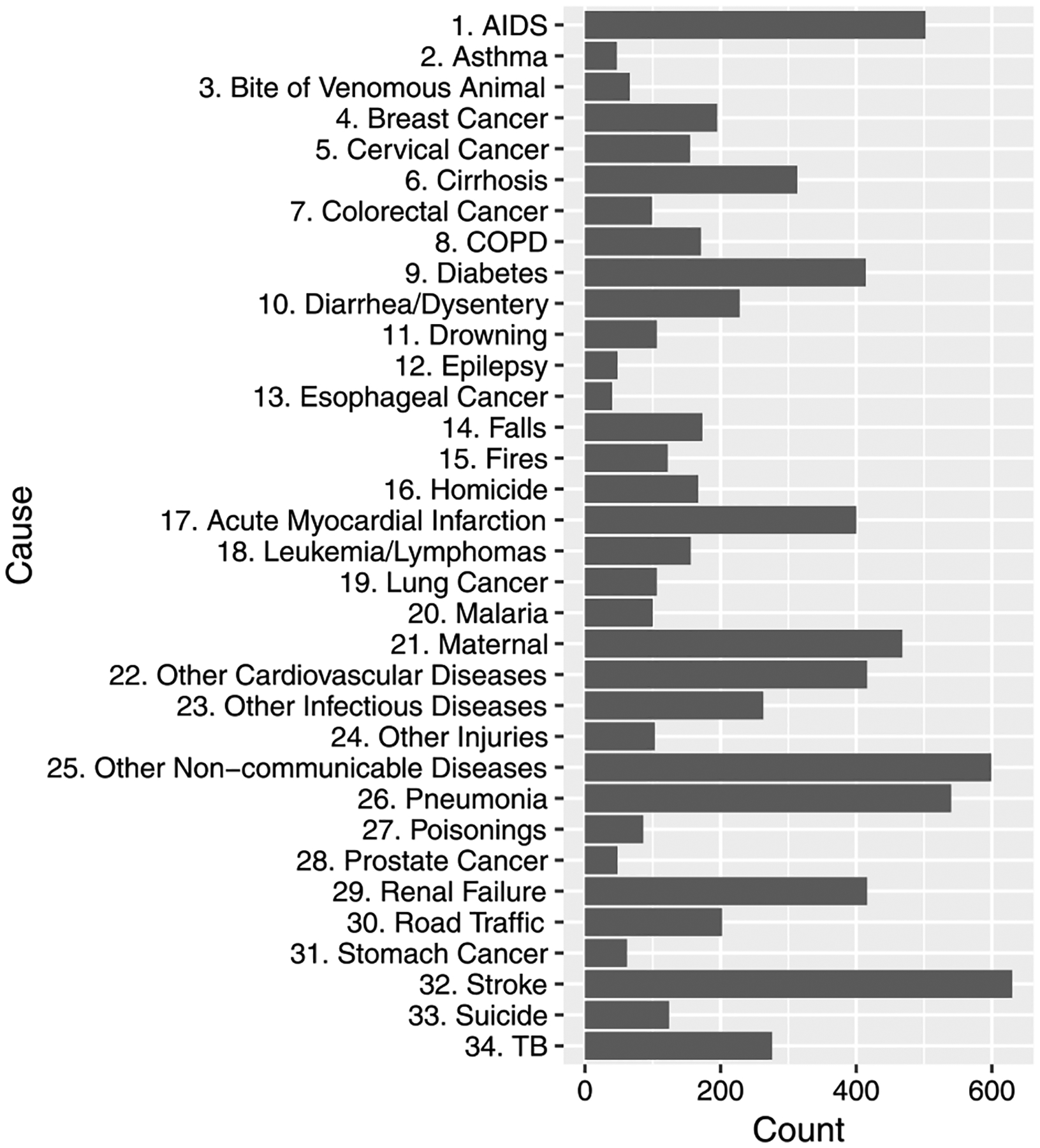
Barplot of 34 causes of death in the PHMRC data. We follow PHMRC (2013) in the numbering of the causes.

Fig. 2.

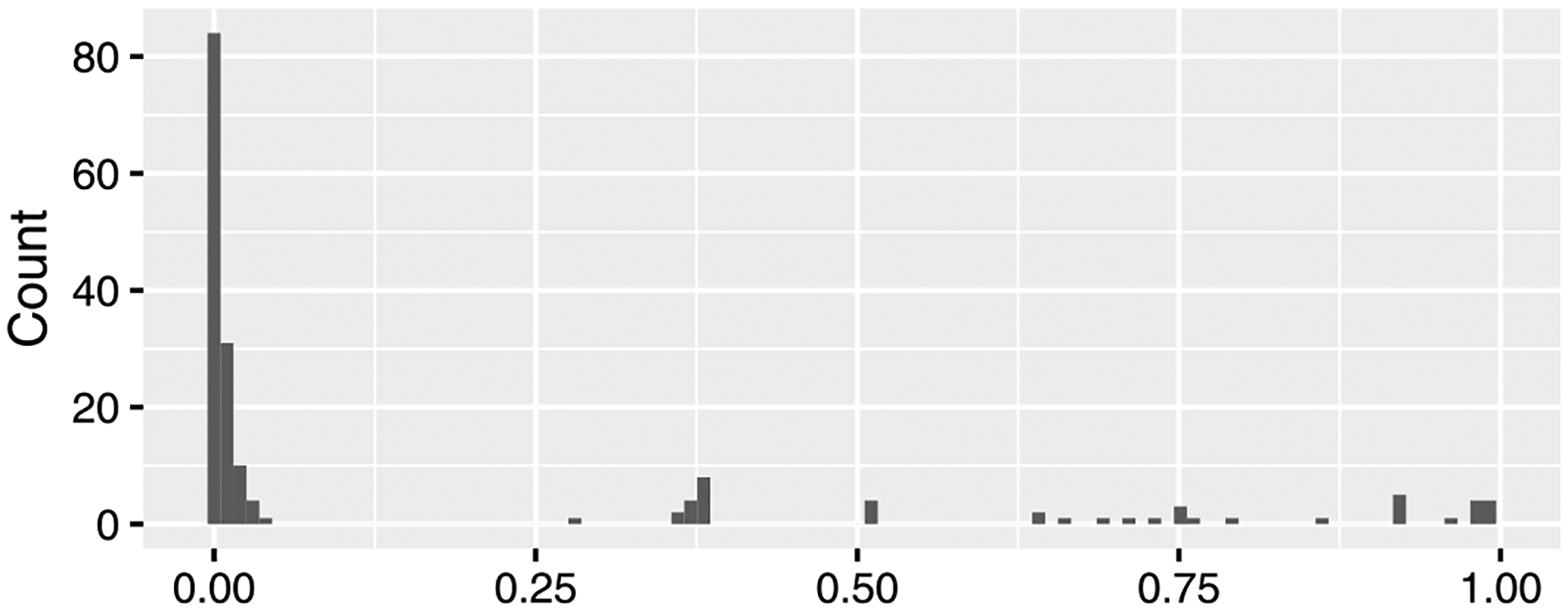
Histogram of the missing rate of the predictors. The horizontal and vertical axes show the missing rate and counts of the predictors.

Since the PHMRC data contain medically-certified causes, we can explore the magnitude of the dependence between symptoms for a given medically-certified cause. We compute Cramér’s V (Cramér (1999)) that measures strength of associations between two variables, taking a value from 0 (no association) to 1 (complete association). Figure 3 shows the result for all pairs of predictors for deaths due to AIDS related causes. We conducted chi-squared test using the R function cramersV in the lsr package (Navarro (2015), R Core Team (2016)), and the hypothesis of independence was rejected with 5% significance level for 1,669 pairs of the predictors out of 15,225 pairs. Using Fisher’s exact test, the hypothesis was rejected with 5% significance level for 1,843 pairs. Unlike most of the previously available methods, our proposed method will utilize these correlations to improve cause assignment accuracy.

Fig. 3.

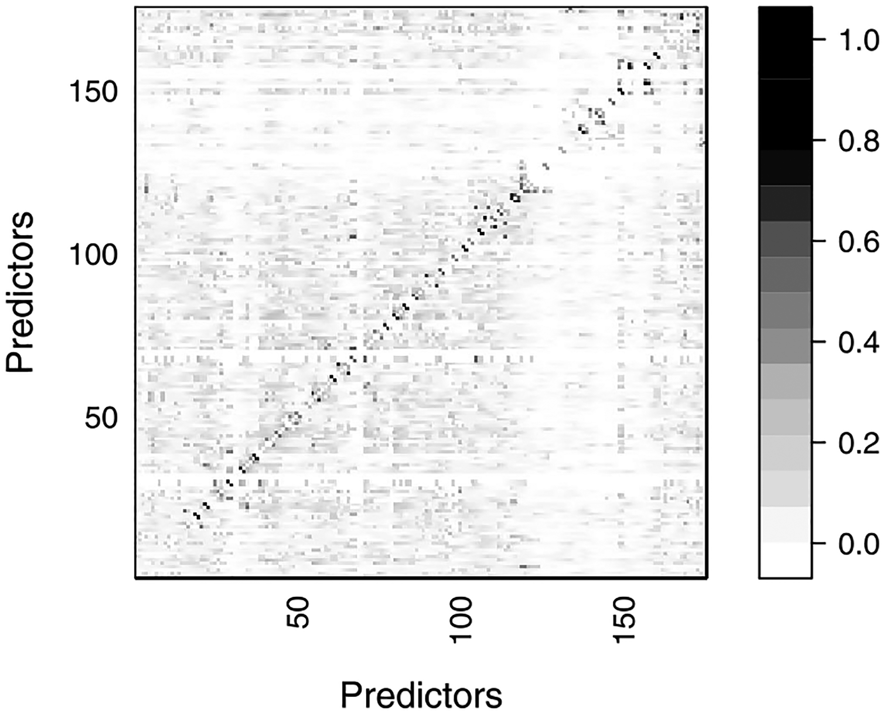
Cramér’s V between predictors for the deaths caused by AIDS. The horizontal and vertical axes present the index of each predictor. Details of the predictors are in the Supplementary Material (Kunihama et al. (2020)). The scale on the right hand side shows the value of Cramér’s V.

2. Bayesian factor model for VA data.

In this section we present our model formulation. First we present the modeling framework, and then we discuss how to assess the importance of symptoms.

2.1. Bayesian approach.

We propose a novel Bayesian framework for assessing cause of death using VA surveys. Let y_i ∈ {1, … , C} be the cause of death of the ith person with i = 1, … , n, and x_i = (x_i1, … , x_ip)′ be the responses to questions j = 1, … , p with x_ij ∈{ 0, 1}. One approach would be to directly build a conditional probability of a person having∈ died from a certain condition given a set of observable covariates π(y_i|x_i) using standard parametric models (e.g., multinomial probit/logit regressions). Modeling these conditional probabilities directly is unappealing, however, since we have a high fraction of missing data (see Figure 2), we would also need to impute a substantial fraction of symptoms. Performing these imputations would require choosing an imputation model, which would bring with it particular assumptions about the structure of the data. Overall, it is not straightforward to build a flexible model for high dimensional binary data with complex interactions, and there is a possibility that the imputation model may fail to capture an actual structure of the data.

Given the challenges with imputing missing values, we opt instead for a Bayesian framework where we can integrate over missing symptoms. To do this, we first express the conditional distribution, π(y_i|x_i), using Bayes’ rule:

$$\pi \left(y_i|x_i\right)=\frac{\pi \left(x_i|y_i\right)\pi \left(y_i\right)}{{\sum }_{c=1}^C\pi \left(x_i|y_i=c\right)\pi \left(y_i=c\right)}.$$

In this framework we can integrate out missing values from π(x_i|y_i). Let $x_i^{\text{obs}}$ and $x_i^{\text{mis}}$ denote the observed and missing items for the ith person with $x_i=\left(x_i^{\text{obs}},x_i^{\text{mis}}\right)$. We assume missing data are missing at random, that is, the probability of the missing-data mechanism depends on observed data but not on the missing values (Rubin (1976), Seaman et al. (2013), Mealli and Rubin (2015)). The PHMRC survey includes a set of questions which first ask about presence of a certain symptom to all respondents. If the respondent has the symptom, then the survey moves to ask about additional details, such as the location of a rash or the severity of a fever. For these questions, the missing-data mechanism can be accounted for at the first question. Under this assumption, one can conduct inference on parameters in a model using only observed information. We utilize the distribution of the cause given the observed items,

$$\pi \left(y_i|x_i^{\text{obs}}\right)\propto \pi \left(x_i^{\text{obs}}|y_i\right)\pi \left(y_i\right)\text{\hspace{0.17em}\hspace{0.17em}\hspace{0.17em}\hspace{0.17em} where\hspace{0.17em}}\pi \left(x_i^{\text{obs}}|y_i\right)=\int \pi \left(x_i|y_i\right)d{x}_i^{\text{mis}}.$$

If the integral can be calculated analytically, we can evaluate the conditional probabilities of the cause on the observed information without imputing missing data. Without assuming missing at random, an additional model is needed to describe the missing-data mechanism. In the case of VA data, however, we do not have the requisite information. Missing data could arise because respondents were asked a question but did not recall the answer. This is expected since the interview is about a traumatic event, requires recalling specialized details and often does not happen until months after the death. Missing data could also arise because interviewers, perhaps with an eye towards a likely cause, strategically asked certain questions or asked questions in a specific order. An active area of research in the VA community involves gathering ethnographic and numeric data to describe the VA interview process, with the hopes of making the process more standard across contexts and understanding missing data mechanisms. Utilizing information about the interview and respondent recall processes, to construct a missing data model still remains an open area of research. Therefore, in the absence of an alternative missing data model, we can enhance the plausibility of the assumption by incorporating as many variables as possible in a model (Little and Rubin (2002), Gelman et al. (2014)).

Under the Bayes rule representation, there are two pieces of the model that we need to specify, (i) the unconditional distribution of individual causes, π(y_i), and (ii) the conditional distribution of observed symptoms given an individual has a particular cause, π(x_i y_i). Beginning with the prior distribution for causes, we assume a Dirichlet distribution,

$$\left\{\pi \left(y_i=1\right),\dots ,\pi \left(y_i=C\right)\right\}~\text{Dirichlet}\left(a_1,\dots ,a_C\right),$$

where a₁, …, a_C are concentration parameters. Since cause patterns can differ substantially across geographic areas and times, we assume we have little prior information about the distribution of causes. We therefore assume a₁ = ⋯ a_C = 1, leading to a uniform prior with π(y_i = c) ∝ 1 for c = 1, … , C.

The second piece, π(x_i|y_i), requires modeling a set of high-dimensional binary predictors given each cause. As described previously, nearly all existing methods for assigning cause of death from verbal autopsies make the assumption of conditional independence across symptoms (Byass et al. (2012), Miasnikof et al. (2015), McCormick et al. (2016)),

$$\pi \left(x_i|y_i\right)=\prod _{j=1}^p\pi \left(x_{ij}|y_i\right).$$

This assumption facilitates computation but disregards substantial and potentially informative relationships between symptoms, as Figure 3 shows.

To flexibly capture dependence, we develop a conditional distribution based on the multivariate probit model. In our framework, each binary outcome is a manifestation of an underlying continuous variable. Let $z_i={\left(z_{i1},\dots ,z_{ip}\right)}^{\prime }\in {ℝ}^p$ be the latent variable for the ith person. We express the multivariate binary variable x_i by transforming the continuous variable z_i. We assume a multivariate normal distribution conditional on a cause, $z_i|y_i~N\left({\mu }_{y_i},{\Sigma }_{y_i}\right)$ with mean ${\mu }_{y_i}={\left({\mu }_{y_{i}1},\dots ,{\mu }_{y_{i}p}\right)}^{\prime }$ and covariance ${\Sigma }_{y_i}$.

Even for moderately large p, estimating p(p + 1)/2 parameters in the covariance matrix will be challenging, particularly since we expect that each dataset will contain only a few deaths by each cause. Further, since our goal is predicting cause of death for a new sample of deaths, we prefer a sparse model to avoid overfitting. Rather than estimating all elements in the covariance matrix, we introduce a K-dimensional factor η_i = (η_i1, …, η_iK)′ with K ≪ p, and propose the following sparse factor model:

$$\begin{gathered} x_{ij}=1\left(z_{ij}>0\right),j=1,\dots ,p, \\ {z}_i={\mu }_{y_i}+{\Lambda }_{y_i}{\eta }_i+{\epsilon }_i,{\eta }_i~N\left(0,I_K\right),{\epsilon }_i~N\left(0,I_p\right), \end{gathered}$$ (1)

where 1(·) is an indicator function and Λ_y = {λ_yjk} is a p ×K loading matrix with y = 1, …, j = 1, …, p and k = 1, …, K. Dependence is induced in z_i by integrating out the factor η_i in (1), leading to the normal distribution with cause-dependent mean and covariance,

$$z_i|y_i~N\left({\mu }_{y_i},{\Lambda }_{y_i}{\Lambda }_{y_i}^{\prime }+I_p\right),$$

where the number of parameters in the covariance reduces from p(p + 1)/2 to Kp. In practice, we will need to choose the number of factors, K, which we propose doing via cross validation. For the prior distribution of the mean and factor loadings, we use Cauchy distributions, a standard shrinkage prior with high density around zero and heavy tails. The Cauchy prior reduces effects of redundant elements, but will also capture meaningful signals. Based on the normal-gamma distribution, we express the Cauchy distribution as

$$\begin{gathered} {\mu }_{yj}~N\left(0,{\tau }_j^{-1}\right),{\tau }_j~\text{Ga}(0.5,0.5), \\ {\lambda }_{yjk}~N\left(0,{\varphi }_j^{-1}\right),{\varphi }_j~\text{Ga}(0.5,0.5), \end{gathered}$$

where Ga(a, b) denotes the gamma distribution with mean a/b. The latent variables τ_j and ϕ_j are shared among the causes and factors for reduction of the number of parameters in the model.

In a factor model, constraints on the factor loadings are necessary to identify the latent factors (Arminger and Muthén (1998), Lopes and West (2004), Zhou, Nakajima and West (2014)). In our context, though, identification is not necessary since the factors are a way to reduce the dimension of the covariance matrix, rather than to be interpreted in and of themselves. We opt not to use constraints for identification since interpreting the factors is not a goal and constraints can lead to order dependence and computational inefficiencies (Bhattacharya and Dunson (2011), Montagna et al. (2012)).

2.2. Measuring strength of association.

VA surveys collect information via questionnaires with many items regarding demographic background, health history and disease symptoms. It can be time-consuming and costly in terms of both enumerator time and the toll on a person close to the decedent to ask redundant questions that will not be useful in predicting likely cause of death. We now propose a method for assessing the importance of each symptom based on the strength of association with causes of death.

For two discrete random variables y ∈ {1, … , m_y} and x ∈ {1, … , m_x}, Dunson and Xing (2009) develop a Bayesian measure of association relying on the parameters which characterize the multivariate distribution,

$${\delta }^2=\frac{1}{\text{min}\left\{m_y,m_x\right\}-1}\times \sum _{c=1}^{m_y}\sum _{d=1}^{m_x}\frac{{\{P(y=c,x=d)-P(y=c)P(x=d)\}}^2}{P(y=c)P(x=d)},$$ (2)

where δ ranges from 0 to 1 with δ ≈ 0 if y and x are independent. If the joint and marginal probabilities are replaced by the empirical distributions, δ will correspond to Cramér’s V. Therefore, δ can be considered a model-based version of Cramér’s V. In the proposed model, it is straightforward to evaluate the probability functions in (2). For example, the joint probability of the cause and jth predictor is expressed as π(y_i, x_ij) = π(x_ij| y_i) π(y_i) where π(x_ij| y_i) is the proposed factor model and π(y_i) is the Dirichlet distribution. In the following section, we describe how the measure can be incorporated into our posterior sampling algorithm.

3. Posterior computation.

The posterior density for the model presented in Section 2.1 is not available in closed form. We instead approximate the posterior density using samples obtained through Markov-chain Monte Carlo (MCMC). Let m_i = (m_i1, … , m_ip)′ be a vector of indicators denoting missing values for the ith person such that m_ij = 1 if x_ij is missing and m_ij = 0 if x_ij is observed with j = 1, …, p. We define notation [m_i] such that, for a vector b and a matrix B with p rows, $b_{[m_i]}$ and $B_{[m_i]}$ denote the subvector and submatrix consisting of components with m_ij = 0 for j = 1, …, p. Then we propose the following MCMC algorithm.

1. Update μ_·j ≡ (μ_1j , …, μ_Cj)′ from N(μ_*,Σ_*) for j = 1, …, p with

   $${\mu }_{*}={\Sigma }_{*}{a}_j,{\Sigma }_{*}=\text{diag}\left\{{\left(n_1+{\tau }_j\right)}^{-1},\dots ,{\left(n_C+{\tau }_j\right)}^{-1}\right\},$$

   where $n_c={\sum }_{i=1}^{n}1\left(y_i=c,m_i=0\right)$ and a_j is the C × 1 vector with the cth element ${\sum }_{i=1}^{n}1\left(y_i=c,m_i=0\right)\left(z_{ij}-{\lambda }_{y_{i}j}^{\prime }.{\eta }_i\right)$ where ${\lambda }_{y_{i}j\cdot }={\left({\lambda }_{y_{i}j1},\dots ,{\lambda }_{y_{i}jK}\right)}^{\prime }$.
2. Update λ_cj· ≡ (λ_cj1, …, λ_cjK)′ from N(μ_λ, Σ_λ) for c = 1, …, C with

   $${\mu }_{\lambda }={\Sigma }_{\lambda }\left\{\sum _{i:y_i=c}{\eta }_i\left(z_{ij}-{\mu }_{y_{i}j}\right)\right\},{\Sigma }_{\lambda }={\left(\sum _{i:y_i=c}{\eta }_i{\eta }_i^{\prime }+{\varphi }_j{I}_K\right)}^{-1}.$$
3. Update η_i from $N(\tilde{\mu },\tilde{\Sigma })$ for i = 1, … , n with

   $$\tilde{\mu }=\tilde{\Sigma }{\Lambda }_{y_i\left[m_i\right]}^{\prime }{\left(z_i-{\mu }_{y_i}\right)}_{\left[m_i\right]},\tilde{\Sigma }={\left({\Lambda }_{y_i\left[m_i\right]}^{\prime }{\Lambda }_{y_i\left[m_i\right]}+I_K\right)}^{-1}.$$
4. Update τ_j for j = 1, …, p from

   $$\text{Ga}\left(\frac{C+1}{2},\frac{{\sum }_{c=1}^C{\mu }_{cj}^2+1}{2}\right).$$
5. Update ϕ_j for j = 1, …, p from

   $$\text{Ga}\left(\frac{CK+1}{2},\frac{{\sum }_{c=1}^C{\sum }_{k=1}^K{\lambda }_{cjk}^2+1}{2}\right).$$
6. Update z_ij with m_ij = 0 for i = 1, …, n and j = 1, …, p from

   $$\{\begin{array}{ll}{N}_{+}\left({\mu }_{y_{i}j}+{\lambda }_{y_{i}j}^{\prime }.{\eta }_i,1\right)\hfill & \text{if }{x}_{ij}=1\hfill \\ N_{-}\left({\mu }_{y_{i}j}+{\lambda }_{y_{i}j}^{\prime }.{\eta }_i,1\right)\hfill & \text{if }{x}_{ij}=0\hfill \end{array}$$

   where N₊ and N₋ denote the truncated normal distributions with support [0,∞) and (−∞, 0] respectively.
7. For a person i ∈ S where S is the target data, generate y_i with

   $$\pi \left(y_i=c|x_i^{\text{obs}}\right)=\frac{\pi \left(x_i^{\text{obs}}|y_i=c\right)\pi \left(y_i=c\right)}{{\sum }_{y=1}^C\pi \left(x_i^{\text{obs}}|y_i=y\right)\pi \left(y_i=y\right)},c=1,\dots ,C,$$

   where $\pi \left(x_i^{\text{obs}}|y_i=c\right)=\int \pi \left(x_i^{\text{obs}}|\eta ,y_i=c\right)f(\eta )d\eta$ is evaluated using a Monte Carlo approximation with η_r ~ N(0, I_K) for r = 1, …, R,

   $$\pi \left(x_i^{\text{obs}}|y_i=c\right)\approx \frac{1}{R}\sum _{r=1}^R\left\{\prod _{j:m_{ij}=0}\pi \left(x_{ij}|{\eta }_r,y_i=c\right)\right\}.$$ (3)
   Then, compute the population distribution of causes of death by

   $$\left(\frac{1}{\#S}\sum _{i\in S}1\left(y_i=1\right),\dots ,\frac{1}{\#S}\sum _{i\in S}1\left(y_i=C\right)\right),$$

   where #S is the number of observations in the test data.

For the estimation of strength of dependence in Section 2.2, Step 7 above is replaced by

7. Update the distribution of causes π(y_i) with Dirichlet(1, …, 1) prior from

$$\text{Dirichlet }\left(\sum _{i=1}^{n}1\left(y_i=1\right)+1,\dots ,\sum _{i=1}^{n}1\left(y_i=C\right)+1\right),$$

and compute δ in (2) for each predictor.

As mentioned previously, we need to specify the number of latent factors, K. In Section 4, we set R = 200 as the number of random samples for the Monte Carlo method in (3) and generated 5000 MCMC samples after the initial 500 samples were discarded as a burn-in period, and every tenth sample was saved. Discarding samples in this way is a widely-used approach known as thinning and is designed to reduce autocorrelations in a Markov chain (Hoff (2009), Gelman et al. (2014)). In addition, thinning is helpful to save computation time in the proposed MCMC algorithm. Step 7 requires the Monte Carlo simulation of the latent factors for computing the conditional probability π(x_i|y_i), which imposes a substantial computational burden. By thinning the chain, one can avoid updating this step at each iteration because the parameters generated in Step 7 do not appear in the other steps. We observed that the sample paths were stable, and the sample autocorrelations dropped smoothly. Illustrative examples of the sample plot and the autocorrelation are in the Supplementary Material (Kunihama et al. (2020)). Replication code for the proposed method is publicly available at https://github.com/kunihama/VA-code.

4. Results.

Using the MCMC algorithm described in the previous section, we fit our model to the PHMRC VA data. We are particularly interested in the improvement that comes from explicitly accounting for dependence between symptoms. We evaluate whether incorporating dependence between symptoms improves prediction of the distribution of deaths by cause in a target population. As an assessment of the performance, we utilize cause specific mortality fraction (CSMF) accuracy, which is a measure of closeness between two probability vectors in the VA literature (McCormick et al. (2016)),

$$\text{CSMF Accuracy}=1-\frac{d_{L_1}\left({\pi }_0,\pi \right)}{2\left\{1-{\text{min}}_{1\le c\le C}{\pi }_0(y=c)\right\}},$$

where $d_{L_1}$ indicates L1 distance between two distributions and $d_{L_1}\left({\pi }_0,\pi \right)={\sum }_{c=1}^C\left|{\pi }_0(y=c)-\pi (y=c)\right|$. It is a transformation of L₁ distance such that a larger value two probability vectors are closer and it equals to 1 if they are the same. The true CSMF, π₀, is approximated by the empirical distribution of causes of death in the test data, and π is the estimated distribution of causes of death by a statistical model. In addition, as another measure of the performance, we compute the correlation between the actual and estimated numbers of deaths per cause.

An important consideration in our evaluation is whether the method works when the cause of death distribution (and possibly the relationship between symptoms and causes) varies between the training and testing set. To be clear, we are assuming that the underlying “true” population relationship between testing and training remains the same, but that we will have limited training data so our model could be highly sensitive to spurious associations between some symptoms and the rare causes that exist in our training sample. This consideration is fundamental in the VA setting since obtaining training data is extremely costly and the fraction of deaths due to each cause can change between testing and training data. For example, in many settings, training data are collected from one geographic area and need to be used for predicting the distribution of deaths by cause at another area. In evaluating the method, we consider realistic scenarios where we estimate the distribution of deaths by cause in one area using training data collected from different geographic areas. We study six scenarios in which each of the PHMRC sites is treated as a target site and the rest together as training data. We observe discrepancies in the distributions of deaths by cause between the test and training data in all scenarios. Especially, the case where the test site is Pemba Island shows a relatively large difference in the distributions of causes. The figure is in the Supplementary Material (Kunihama et al. (2020)).

For the proposed method, we selected an optimal number of latent factors by fivefold cross-validation. Figure 4 reports the result, indicating 5 or 6 factors are enough for each scenario. We compare the proposed method with state of the art VA classification algorithms. In addition to the conditionally independent model, we employ methods currently used in practice: InSilicoVA (McCormick et al. (2016)), InterVA Byass et al. (2012), King–Lu (King and Lu (2008), King, Lu and Shibuya (2010)) and Tariff (James, Flaxman and Murray (2011), Serina et al. (2015)). These methods assign causes without the information about constellations or clusters of symptoms. King–Lu is the exception that takes into account dependence between symptoms but it can incorporate only a small subset of symptoms at a time. On the other hand, the proposed method can jointly model all predictors without the assumption of conditional independence. Details of the competitors are in the Supplementary Material (Kunihama et al. (2020)).

Fig. 4.

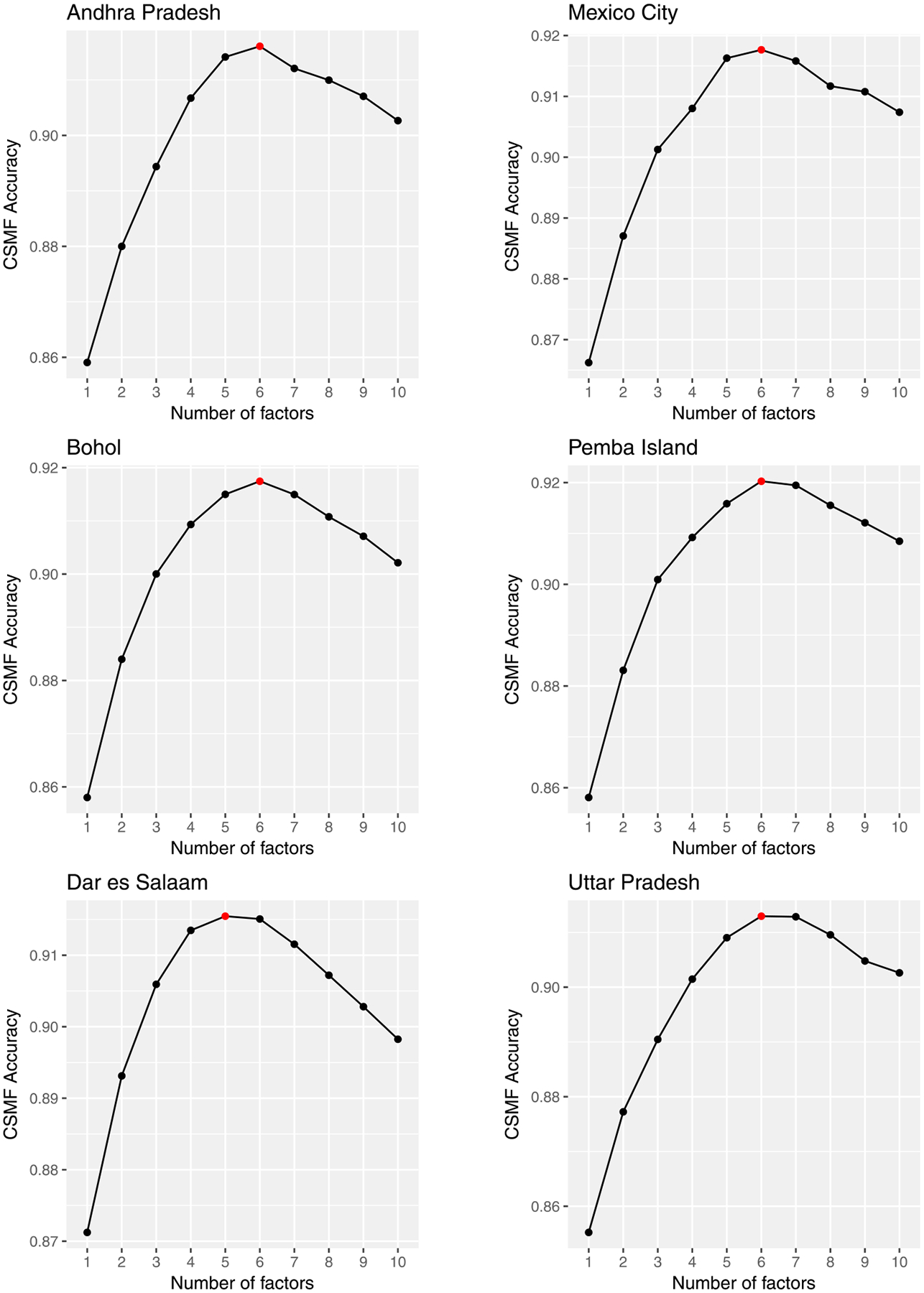
Estimation result of fivefold cross validation in the scenarios where the target sites are Andhra Pradesh (top left), Bohol (middle left), Dar es Salaam (bottom left), Mexico City (top right), Pemba Island (middle right) and Uttar Pradesh (bottom right). The horizontal and vertical axes represent the number of factors and the posterior mean of CSMF accuracy. The red circle indicates the point with the highest accuracy.

Figure 5 reports the boxplot of CSMF accuracy for each scenario. It shows the proposed method works well, producing the accuracy equal to or higher than the competitors in all scenarios. As for the competitors, the order changes in each scenario, and InterVA and Tariff often report small values. Although King–Lu takes into account dependence between symptoms, the performance can be lower than the other competitors with the assumption of conditional independence. This is probably because it relies on modeling of small subsets of predictors. All the methods show relatively low values in the scenario where the target site is Pemba Island with the largest gap of the distributions of causes between the target and training sites. Figure 6 shows the boxplot of correlation between the actual and predicted numbers of deaths per cause. The result is similar in that the proposed method works as well as or better than the competitors in all scenarios, and the values are relatively small for all the methods in the scenario with the target site Pemba Island. In addition, we conduced the sensitivity analysis of the prior and the number of random samples in (3) for the proposed method and obtained stable results given in the Supplementary Material (Kunihama et al. (2020)).

Fig. 5.

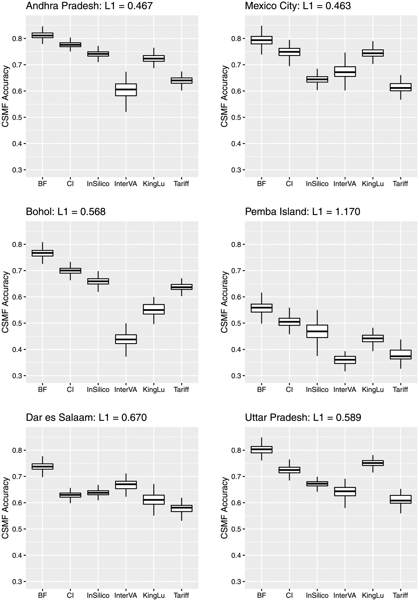
Boxplot of CSMF accuracy by Bayesian factor model (BF), conditionally independent model (CI), InSilicoVA (InSilico), InterVA, King–Lu method (KingLu) and Tariff for scenarios where the target sites are Andhra Pradesh (top left), Bohol (middle left), Dar es Salaam (bottom left), Mexico City (top right), Pemba Island (middle right) and Uttar Pradesh (bottom right). For each scenario, L1 indicates L₁ distance between the empirical distributions in the test and training data. A larger L₁ distance means a larger difference between the distributions.

Fig. 6.

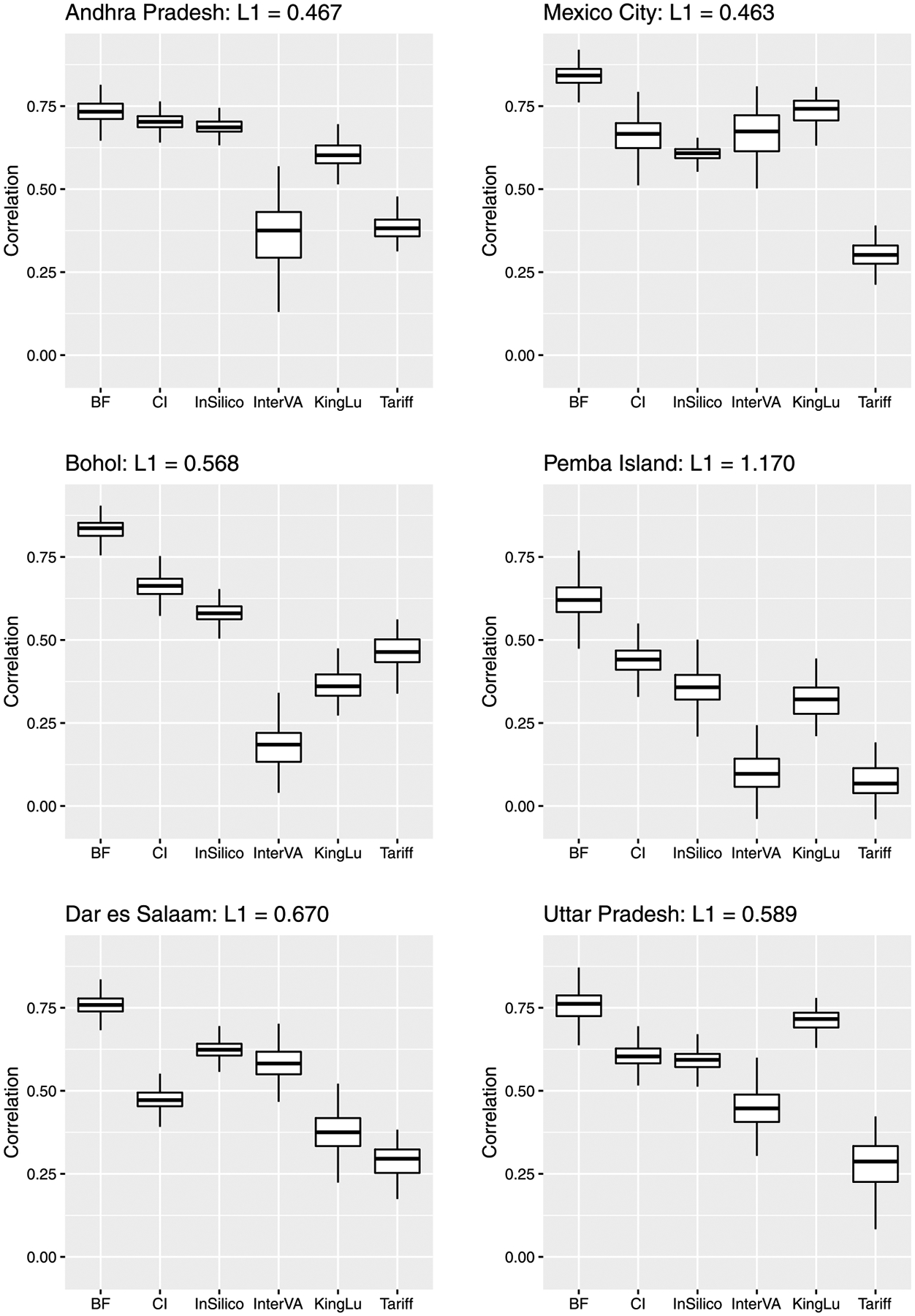
Boxplot of correlation between the actual and predicted numbers of deaths per cause by Bayesian factor model (BF), conditionally independent model (CI), InSilicoVA (InSilico), InterVA, King–Lu method (KingLu) and Tariff for scenarios where the target sites are Andhra Pradesh (top left), Bohol (middle left), Dar es Salaam (bottom left), Mexico City (top right), Pemba Island (middle right) and Uttar Pradesh (bottom right). For each scenario, L1 indicates L₁ distance between the empirical distributions in the test and training data. A larger L₁ distance means a larger difference between the distributions.

Turning now to results for the measure of strength of association between the causes and predictors, we estimate δ in Section 2.2 using the proposed model. As in Figure 2, some items show high missing rates, and to obtain robust results, we include only predictors with a missing rate less than 5%. Figure 7 reports the boxplot of δ for top 15 predictors. We observe that several items related to medical history show high dependence such as cancer and TB. There are also other types of items in the list. For example, predictors 140, 146, 147 are questions for women about pregnancy and childbirth, and predictors 171 and 172 are about injuries. The estimation result of δ for other predictors are in the Supplementary Material (Kunihama et al. (2020)). In addition, we compute the dependence measure in a cause-specific way by transforming the original variable with 34 causes into a binary variable taking 1 for a certain cause and 0 for the rest. The result indicates that important predictors vary with each cause. For example, a set of questions related to paralysis show relatively strong dependence with stroke, while the association of the medical history is much higher than other predictors in AIDS. These results are in the Supplementary Material (Kunihama et al. (2020)).

Fig. 7.

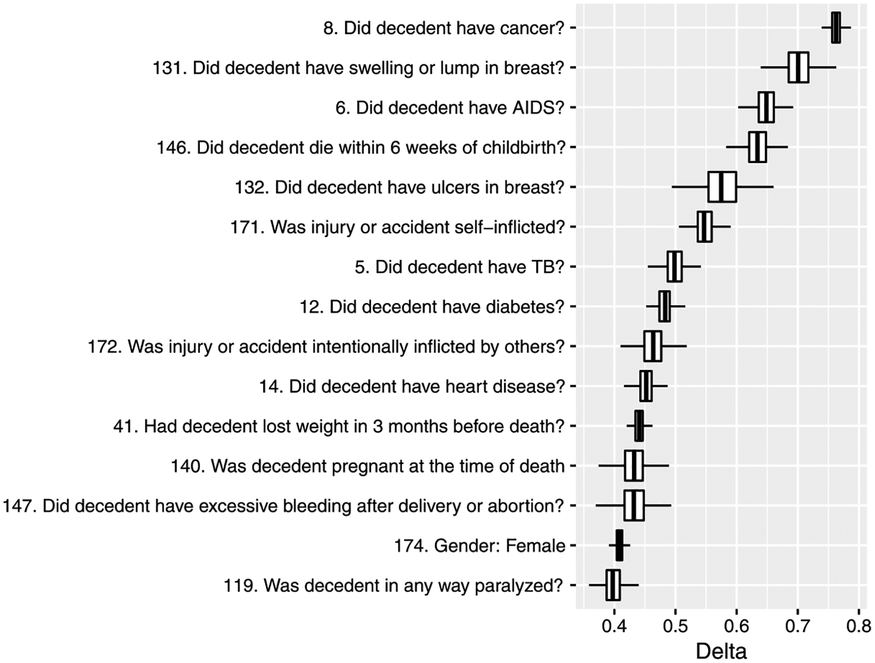
Boxplot of δ for top 15 predictors in descending order of the posterior mean. The index of each predictor is in the Supplementary Material (Kunihama et al. (2020)).

5. Discussion.

In the VA literature, there have been various statistical approaches for estimation of population distributions of causes of death. The key is how to model high dimensional binary predictors given a cause with many missing values. For simplicity, existing methods analyze survey data under strong assumptions such as conditional independence between symptoms. The contribution of this article is to analyze the PHMRC data using a new Bayesian method that flexibly captures complex interactions between symptoms without the restrictive assumption. In the proposed framework, one can measure strength of dependence of each symptom with the causes, which can be useful for the selection of questionnaire items in a future survey.

One future direction is to incorporate spatial information into the proposed model. Factors affecting cause of death vary through space depending on geographic characteristics, so two sites that are close to each other should largely share the same factors affecting cause of death. Therefore it may be more efficient to estimate distributions of deaths by cause by weighting more on neighboring areas. In addition the relationship between causes and questionnaire items may depend on space. Although this article assumes the conditional distribution of the symptoms given a cause is constant over space, one can extend it to π(x|y, s) with spatial information s.

Another direction for future work is to generalize the proposed framework for survey weights. To save cost and time many social surveys employ special data-collection designs such as stratified sampling that produce a biased sample. To adjust for a gap between the sample and the population, survey weights are constructed and distributed along with the data. When faced with data like that, it is necessary to incorporate the weights into statistical models for prediction.

In the proposed approach, the original mixed-scale questions are transformed into multivariate binary variables. However, the assumption of all predictors being binary may be too restrictive. For example, age is considered to be closely related with death but the process of dichotomization may conceal its effects on causes of death. Therefore, one can improve estimation of distributions of causes of death by extending the proposed framework to allow the predictors to have different scales.

REFERENCES

- AbouZahr C, Cleland J, Coullare F, Macfarlane SB, Notzon FC, Setel P, Szreter S, Anderson RN, Bawah AA et al. (2007). The way forward. Lancet 370 1791–1799. [DOI] [PubMed] [Google Scholar]
- Arminger G and Muthén BO (1998). A Bayesian approach to nonlinear latent variable models using the Gibbs sampler and the Metropolis–Hastings algorithm. Psychometrika 63 271–300. [Google Scholar]
- Bhattacharya A and Dunson DB (2011). Sparse Bayesian infinite factor models. Biometrika 98 291–306. MR2806429 10.1093/biomet/asr013 [DOI] [PMC free article] [PubMed] [Google Scholar]
- Bloomberg MR and Bishop J (2015). Understanding death, extending life. Lancet 386 e18–e19. [DOI] [PubMed] [Google Scholar]
- Byass P, Chandramohan D, Clark SJ, D’Ambruoso L, Fottrell E, Graham WJ, Herbst AJ, Hodgson A, Hounton S et al. (2012). Strengthening standardised interpretation of verbal autopsy data: The new InterVA-4 tool. Global Health Action 5 19281. [DOI] [PMC free article] [PubMed] [Google Scholar]
- Cramér H (1999). Mathematical Methods of Statistics Princeton Landmarks in Mathematics. Princeton Univ. Press, Princeton, NJ: MR1816288 [Google Scholar]
- De Savigny D, Riley I, Chandramohan D, Odhiambo F, Nichols E, Notzon S, AbouZahr C, Mitra R, Cobos Muñoz D et al. (2017). Integrating community-based verbal autopsy into civil registration and vital statistics (crvs): System-level considerations. Global Health Action 10 1272882. [DOI] [PMC free article] [PubMed] [Google Scholar]
- Doornik JA (2007). Object-oriented matrix programming using Ox, 3rd ed. Timberlake Consultants, London, and www.doornik.com, Oxford. [Google Scholar]
- Dunson DB and Xing C (2009). Nonparametric Bayes modeling of multivariate categorical data. J. Amer. Statist. Assoc 104 1042–1051. MR2562004 10.1198/jasa.2009.tm08439 [DOI] [PMC free article] [PubMed] [Google Scholar]
- Gelman A, Carlin JB, Stern HS, Dunson DB, Vehtari A and Rubin DB (2014). Bayesian Data Analysis, 3rd ed. Texts in Statistical Science Series. CRC Press, Boca Raton, FL: MR3235677 [Google Scholar]
- Hoff PD (2009). A First Course in Bayesian Statistical Methods Springer Texts in Statistics. Springer, New York: MR2648134 10.1007/978-0-387-92407-6 [DOI] [Google Scholar]
- Horton R (2007). Counting for health. Lancet 370 1526 10.1016/S0140-6736(07)61418-4 [DOI] [PubMed] [Google Scholar]
- James SL, Flaxman AD and Murray CJ (2011). Performance of the Tariff Method: Validation of a simple additive algorithm for analysis of verbal autopsies. Population Health Metrics 9 31. [DOI] [PMC free article] [PubMed] [Google Scholar]
- Jha P (2014). Reliable direct measurement of causes of death in low-and middle-income countries. BMC Medicine 12 19. [DOI] [PMC free article] [PubMed] [Google Scholar]
- King G and Lu Y (2008). Verbal autopsy methods with multiple causes of death. Statist. Sci 23 78–91. MR2523943 10.1214/07-STS247 [DOI] [Google Scholar]
- King G, Lu Y and SHIBUYA K (2010). Designing verbal autopsy studies. Population Health Metrics 8 19. [DOI] [PMC free article] [PubMed] [Google Scholar]
- Kunihama T, Li ZR, Clark SJ and McCormick TH (2020). Supplement to “Bayesian factor models for probabilistic cause of death assessment with verbal autopsies.” 10.1214/19-AOAS1253SUPPA, . [DOI] [PMC free article] [PubMed]
- Little RJA and Rubin DB (2002). Statistical Analysis with Missing Data, 2nd ed. Wiley Series in Probability and Statistics. Wiley, Hoboken, NJ: MR1925014 10.1002/9781119013563 [DOI] [Google Scholar]
- Lopes HF and West M (2004). Bayesian model assessment in factor analysis. Statist. Sinica 14 41–67. MR2036762 [Google Scholar]
- Lopez AD (1998). Counting the dead in China. BMJ 317 1399–1400. [DOI] [PMC free article] [PubMed] [Google Scholar]
- Lozano R, Lopez AD, Atkinson C, Naghavi M, Flaxman AD and Murray CJ (2011). Performance of physician-certified verbal autopsies: Multisite validation study using clinical diagnostic gold standards. Population Health Metrics 9 32. [DOI] [PMC free article] [PubMed] [Google Scholar]
- Maher D, Biraro S, Hosegood V, Isingo R, Lutalo T, Mushati P, Ngwira B, Nyirenda M, Todd J et al. (2010). Translating global health research aims into action: The example of the ALPHA network. Tropical Medicine & International Health 15 321–328. [DOI] [PubMed] [Google Scholar]
- Mathers CD, Fat DM, Inoue M, Rao C and Lopez AD (2005). Counting the dead and what they died from: An assessment of the global status of cause of death data. Bulletin of the World Health Organization 83 171–177. [PMC free article] [PubMed] [Google Scholar]
- McCormick TH, Li ZR, Calvert C, Crampin AC, Kahn K and Clark SJ (2016). Probabilistic cause-of-death assignment using verbal autopsies. J. Amer. Statist. Assoc 111 1036–1049. MR3561927 10.1080/01621459.2016.1152191 [DOI] [PMC free article] [PubMed] [Google Scholar]
- Mealli F and Rubin DB (2015). Clarifying missing at random and related definitions, and implications when coupled with exchangeability. Biometrika 102 995–1000. MR3431570 10.1093/biomet/asv035 [DOI] [Google Scholar]
- Miasnikof P, Giannakeas V, Gomes M, Aleksandrowicz L, Shestopaloff AY, Alam D, Tollman S, Samarikhalaj A and Jha P (2015). Naive Bayes classifiers for verbal autopsies: Comparison to physician-based classification for 21,000 child and adult deaths. BMC Medicine 13 286. [DOI] [PMC free article] [PubMed] [Google Scholar]
- Mikkelsen L, Phillips DE, Abouzahr C, Setel PW, De Savigny D, Lozano R and Lopez AD (2015). A global assessment of civil registration and vital statistics systems: Monitoring data quality and progress. Lancet 386 1395–1406. [DOI] [PubMed] [Google Scholar]
- Montagna S, Tokdar ST, Neelon B and Dunson DB (2012). Bayesian latent factor regression for functional and longitudinal data. Biometrics 68 1064–1073. MR3040013 10.1111/j.1541-0420.2012.01788.x [DOI] [PMC free article] [PubMed] [Google Scholar]
- Murray CJ, Lopez AD, Black R, Ahuja R, Ali SM, Baqui A, Dandona L, Dantzer E, Das V et al. (2011). Population Health Metrics Research Consortium gold standard verbal autopsy validation study: Design, implementation, and development of analysis datasets. Population Health Metrics 9 27. [DOI] [PMC free article] [PubMed] [Google Scholar]
- Navarro D (2015). Learning statistics with R: A tutorial for psychology students and other beginners. (Version 0.5). Univ. Adelaide Available at http://ua.edu.au/ccs/teaching/lsr.
- Nichols EK, Byass P, Chandramohan D, Clark SJ, Flaxman AD, Jakob R, Leitao J, Maire N, Rao C et al. (2018). The WHO 2016 verbal autopsy instrument: An international standard suitable for automated analysis by InterVA, InSilicoVA, and Tariff 2.0. PLoS. Medicine 15 e1002486. [DOI] [PMC free article] [PubMed] [Google Scholar]
- Phillips DE, AbouZahr C, Lopez AD, Mikkelsen L, De Savigny D, Lozano R, Wilmoth J and Setel PW (2015). Are well functioning civil registration and vital statistics systems associated with better health outcomes? Lancet 386 1386–1394. [DOI] [PubMed] [Google Scholar]
- PHMRC (2013). Population Health Metrics Research Consortium gold standard verbal autopsy data 2005–2011. Available at http://ghdx.healthdata.org/record/population-health-metrics-research-consortium-gold-standard-verbal-autopsy-data-2005-2011. [DOI] [PMC free article] [PubMed]
- R Core Team (2016). R: A Language and Environment for Statistical Computing. R Foundation for Statistical Computing, Vienna, Austria: Available at https://www.R-project.org/. [Google Scholar]
- Rubin DB (1976). Inference and missing data. Biometrika 63 581–592. MR0455196 10.1093/biomet/63.3.581 [DOI] [Google Scholar]
- Ruzicka LT and Lopez AD (1990). The use of cause-of-death statistics for health situation assessment: National and international experiences. World Health Statistics Quarterly 43 249–258. [PubMed] [Google Scholar]
- Sankoh O and Byass P (2012). The INDEPTH Network: Filling vital gaps in global epidemiology. Int. J. Epidemiol 41 579–588. [DOI] [PMC free article] [PubMed] [Google Scholar]
- Seaman S, Galati J, Jackson D and Carlin J (2013). What is meant by “missing at random”? Statist. Sci 28 257–268. MR3112409 10.1214/13-sts415 [DOI] [Google Scholar]
- Serina P, Riley I, Stewart A, James SL, Flaxman AD, Lozano R, Hernandez B, Mooney MD, Luning R et al. (2015). Improving performance of the Tariff Method for assigning causes of death to verbal autopsies. BMC Medicine 13 291. [DOI] [PMC free article] [PubMed] [Google Scholar]
- Soleman N, Chandramohan D and Shibuya K (2006). Verbal autopsy: Current practices and challenges. Bulletin of the World Health Organization 84 239–245. [DOI] [PMC free article] [PubMed] [Google Scholar]
- World Health Organization (2012). Verbal Autopsy Standards: The 2012 WHO verbal autopsy instrument. Available at https://goo.gl/bQXXhG.
- World Health Organization (2017). Verbal Autopsy Standards: The 2016 WHO verbal autopsy instrument. Available at https://goo.gl/Hgt6es.
- Yang G, HU J, RAO KQ, MA J, RAO C and LOPEZ AD (2005). Mortality registration and surveillance in China: History, current situation and challenges. Population Health Metrics 3 3. [DOI] [PMC free article] [PubMed] [Google Scholar]
- Zhou X, NAKAJIMA J and WEST M (2014). Bayesian forecasting and portfolio decisions using dynamic dependent sparse factor models. Int. J. Forecast 30 963–980. [Google Scholar]
Associated Data
This section collects any data citations, data availability statements, or supplementary materials included in this article.