Robust inference on population indirect causal effects: the generalized front door criterion

Summary.

Standard methods for inference about direct and indirect effects require stringent no-unmeasured-confounding assumptions which often fail to hold in practice, particularly in observational studies. The goal of the paper is to introduce a new form of indirect effect, the population intervention indirect effect, that can be non-parametrically identified in the presence of an unmeasured common cause of exposure and outcome. This new type of indirect effect captures the extent to which the effect of exposure is mediated by an intermediate variable under an intervention that holds the component of exposure directly influencing the outcome at its observed value. The population intervention indirect effect is in fact the indirect component of the population intervention effect, introduced by Hubbard and Van der Laan. Interestingly, our identification criterion generalizes Judea Pearl’s front door criterion as it does not require no direct effect of exposure not mediated by the intermediate variable. For inference, we develop both parametric and semiparametric methods, including a novel doubly robust semiparametric locally efficient estimator, that perform very well in simulation studies. Finally, the methods proposed are used to measure the effectiveness of monetary saving recommendations among women enrolled in a maternal health programme in Tanzania.

1. Introduction

The population-average causal effect is by and large the most common form of total effect evaluated in observational data because of the natural connection to scientific queries arising from randomized studies. However, alternative forms of total effect may be of greater interest in observational studies with harmful exposure such that one may not want to conceive of a hypothetical intervention that forces a person to be exposed. Hubbard and Van der Laan (2008) defined the population intervention effect (PIE) of an exposure as the contrast relating the mean of an outcome in the population to that in the same observed population if no one had been exposed. Interestingly, the PIE is closely related to the effect of treatment on the treated (ETT) and attributable fraction (AF), which have also been toted as causal quantities to assess public health impact of a harmful exposure (Geneletti and Dawid, 2011; Hahn, 1998; Sjölander and Vansteelandt, 2010; Greenland and Drescher, 1993). The ETT compares the outcome among those exposed with the potential outcome if they had not been exposed—for binary treatment, the PIE is equal to the ETT scaled by prevalence of treated individuals. The AF is the proportion of potential outcome events that would be eliminated from the observed population if contrary to fact no one had been exposed—for binary outcomes, the PIE is equal to the AF scaled by prevalence of outcome. As such, the PIE is relative to the distribution of an exposure in the population of interest and may be of greater interest when evaluating the potential effect of programmes that eliminate a harmful exposure from a population.

Recent causal mediation methods have been developed to decompose such total causal effects into direct and indirect pathways through a mediating variable (Pearl, 2001; Vansteelandt and VanderWeele, 2012; Sjölander, 2018). Although the natural (pure) direct and indirect effects of the average causal effect (ACE) are the most common form of mediated causal effects, researchers have argued that the direct and indirect components of the ETT and AF are equally of scientific interest and may in fact require weaker conditions for identification (Vansteelandt and VanderWeele, 2012). Namely, identification of natural direct and indirect effects requires the stringent assumption that there is no unmeasured confounding of the exposure–outcome, exposure–mediator and mediator–outcome associations and no exposure-induced confounding of the mediator–outcome association, even by measured factors (Pearl, 2001; Avin et al., 2005). Vansteelandt and VanderWeele (2012) proposed a particular form of direct and indirect effects of the ETT which they showed remain identified in the presence of exposure–mediator unmeasured confounding. This is an important result for settings where a randomized experiment is impractical or unethical such that observational data must be used and unmeasured confounding effects of the exposure cannot be ruled out. Unfortunately, Vansteelandt and VanderWeele (2012) could not identify the indirect effect whenever the exposure–outcome association is confounded. In this paper, we propose an alternative form of indirect effect and describe sufficient conditions for non-parametric identification in the presence of unmeasured confounding of the exposure–outcome association, therefore complementing the results of Vansteelandt and VanderWeele (2012).

Specifically, we propose a decomposition of the PIE into the population intervention direct effect (PIDE) and population intervention indirect effect (PIIE). The PIIE is interpreted as the contrast between the observed outcome mean for the population and the population outcome mean if contrary to fact the mediator had taken the value that it would have in the absence of exposure. Thus, the PIIE is relative to the current distribution of an exposure and does not require conceiving of an intervention that would force an individual to take a harmful level of exposure in the case of binary exposure (Hubbard and Van der Laan, 2008). Our approach leads to an alternative effect decomposition of the ETT and AF of Vansteelandt and VanderWeele (2012) and Sjölander (2018) (up to a scaling factor). Notably, we establish that the PIIE can be identified even when there is an unmeasured common cause of exposure and outcome variables, provided that it is not also a cause of the mediator. This estimand may be of interest in a variety of settings where unmeasured confounding of the exposure–outcome relationship cannot be ruled out with certainty. For example, in recommender systems, the assignment mechanism for the mediator (e.g. recommendation) is typically known or under the control of the researcher, such that unmeasured confounding of the exposure–mediator and mediator–outcome relationships are not of concern. The application that is considered in this paper investigates the indirect effect of a woman’s risk of pregnancy on monetary savings for delivery mediated by the amount that she is recommended to save by a community health worker. Note that the PIDE does not share this identification result and is identified under the same conditions as the natural direct effect (NDE).

Beyond its inherent scientific interest as quantifying the mediated component of the PIE, the PIIE may also be viewed as an approach to identify partially a total effect of an exposure on an outcome subject to unmeasured confounding in settings where one might be primarily interested in such a total effect. Interestingly, the identifying formula that we obtain for the PIIE matches Judea Pearl’s celebrated front door formula: a well-known result for identification of the total effect in the presence of unmeasured confounding given that

1. a mediating variable(s) intercepts all directed paths from exposure to outcome so that the indirect effect equals the total effect and

2. there is no unmeasured confounding of the mediator–outcome or exposure–mediator associations (Pearl, 2009).

In the setting where an investigator believes that they have captured one or more mediating variables that satisfy the front door criterion, they can use our proposed methodology to estimate either the PIE or the ACE. Notably, identification of indirect effects with Pearl’s front door criterion requires a key assumption of no direct effect of the exposure on the outcome not through the mediator in view. In contrast, our generalized front door criterion allows for such direct effects. Thus, even if an investigator cannot satisfy criterion (a), they may still be able to capture the unconfounded component of the PIE through one or more mediating variables. Compared with other methods that relax the assumption of no unmeasured confounding to identify causal effects, our approach applies more generally as it does not require a valid instrumental variable, measuring one or more negative control variables, or parametric assumptions for identification (Angrist et al., 1996; Imbens and Lemieux, 2008; Campbell and Stanley, 1963; Lipsitch et al., 2010; Miao and Tchetgen Tchetgen, 2017; VanderWeele and Arah, 2011). We emphasize that, whereas the front door criterion has long been established, the proposed generalized front door criterion is entirely new to the literature. In addition to new identification results, we also develop both parametric and semiparametric theory for inference about the PIIE. To the best of our knowledge, the methodology proposed also delivers the first doubly robust estimator of Pearl’s front door formula in the literature.

The rest of the paper is organized as follows: in Section 2, we discuss non-parametric identification of the PIIE and PIDE. In Section 3, we derive both parametric and semiparametric estimators, including a doubly robust semiparametric locally efficient estimator for the PIIE and PIDE. In Section 4, the performance of these estimators is evaluated in a range of settings in extensive simulation studies. In Section 5, the methods proposed are used to measure the effectiveness of monetary savings recommendations for delivery among pregnant women enrolled in a maternal health programme in Zanzibar, Tanzania.

2. Non-parametric identification

In what follows, let Z(a) denote the counterfactual mediator variable if the exposure had taken value a and Y(a) = Y{a, Z(a)} denote the counterfactual outcome if exposure possibly contrary to the fact had taken value a. We shall also consider the counterfactual outcome Y{A, Z(a*)} = Y{Z(a*)} if exposure had taken its natural level and the mediator variable taken the value that it would have under a*. When a* = 0, Y{Z(0)} is the counterfactual outcome if exposure had taken its natural level and the mediator variable taken the value that it would have under no exposure. Additionally, let C be a set of observed pre-exposure covariates known to confound A–Z-, A–Y - and Z–Y -associations. Throughout Z can be vector valued.

We first consider the standard decomposition of the ACE. For exposure levels a and a*,

$$\begin{gathered} \text{ACE}\left(a,a^{*}\right)=E\left[Y\left\{a,Z\left(a\right)\right\}-Y\left\{a^{*},Z\left(a^{*}\right)\right\}\right] \\ =\underset{\text{NIE}}{\underbrace{E\left[Y\left\{a,Z\left(a\right)\right\}-Y\left\{a,Z\left(a^{*}\right)\right\}\right]}}+\underset{\text{NDE}}{\underbrace{E\left[Y\left\{a,Z\left(a^{*}\right)\right\}-Y\left\{a^{*},Z\left(a^{*}\right)\right\}\right]}}. \end{gathered}$$

The natural indirect effect (NIE) is the difference between the potential outcome under exposure value a and the potential outcome if exposure had taken value a but the mediator variable had taken the value that it would have under a*:

$$\text{NIE}\left(a,a^{*}\right)=E\left[Y\left\{a,Z\left(a\right)\right\}-Y\left\{a,Z\left(a^{*}\right)\right\}\right].$$

The NDE is therefore given by ACE(a, a*) − NIE(a, a*). The NIE and NDE are well known to be identified under the following conditions (Pearl, 2012; Imai et al., 2010a).

Assumption 1 (consistency assumptions).

1. If A = a, then Z(a) = Z with probability 1.

2. If A = a, then Y(a) = Y with probability 1.

3. If A = a and Z = z, then Y(a, z) = Y with probability 1.

Assumption 2.

Z(a*) ⊥ A|C = c ∀ a*, c.

Assumption 3.

Y(a, z) ⊥ Z(a*)|A = a, C = c ∀ z, a, a*, c.

Assumption 4.

Y(a, z) ⊥ A|C = c ∀ z, a, c.

Assumption 1 states that the observed outcome is equal to the counterfactual outcome corresponding to the observed treatment. The remaining assumptions essentially state that there is no unmeasured confounding of the exposure and the mediator variable (assumption 2), the mediator variable and the outcome (assumption 3), and the exposure and the outcome (assumption 4). In addition, assumption 3 rules out exposure-induced mediator–outcome confounding. These assumptions could equivalently be formulated under a non-parametric structural equation model (NPSEM) with independent errors (IEs) interpretation of Fig. 1(a) (Pearl, 2009). In addition, define the following positivity assumptions.

Fig. 1.

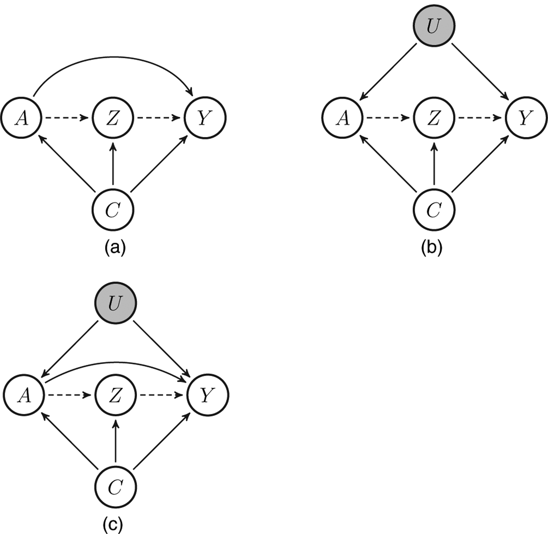
Causal diagrams with indirect effects () (the following indirect effects are identified in each diagram under an NPSEM with IEs (Pearl, 2009) interpretation of the diagram: (a) NIE and PIIE; (b) NIE (equal to the total effect) and PIIE (equal to the PIE); (c) PIIE; further, the indirect effects in (b) are identified under a finest fully randomized causally interpretable structured tree graph (Robins, 1986), which does not encode so-called ‘cross-world’ assumptions such as assumption 3)

Condition 1.

There exists m₁ > 0 such that f(Z|A, C) > m₁ almost surely.

Condition 2.

There exists m₂ > 0 such that f(A|C) > m₂ almost surely.

Here f(Z|A, C) and f(A|C) are the probability density functions for Z|A,C and A|C respectively. Under assumptions 1–4 and the positivity conditions 1 and 2,

$$E\left[Y\left\{a,Z\left(a^{*}\right)\right\}\right]=\sum _{c,z}E\left(Y\mid A=a,Z=z,C=c\right)\text{Pr}\left(Z=z\mid A=a^{*},C=c\right)\text{Pr}\left(C=c\right).$$ (1)

The NIE and NDE fail to be non-parametrically identified if any of assumptions 1–4 fail to hold without an additional assumption (Imai et al., 2010b; Shpitser, 2013).

We shall now formally define the decomposition of the PIE under exposure value a*:

$$\begin{gathered} \text{PIE}\left(a^{*}\right)=E\left[Y\left\{A,Z\left(A\right)\right\}-Y\left(a^{*}\right)\right] \\ =\underset{\text{PIIE }}{\underbrace{E\left[Y\left\{A,Z\left(A\right)\right\}-Y\left\{A,Z\left(a^{*}\right)\right\}\right]}}+\underset{\text{PIDE }}{\underbrace{E\left[Y\left\{A,Z\left(a^{*}\right)\right\}-Y\left\{a^{*},Z\left(a^{*}\right)\right\}\right]}} \end{gathered}$$

The PIIE is a novel measure of indirect effect corresponding to the effect of an intervention which changes the mediator from its natural value (i.e. its observed value) to the value that it would have had under exposure value a*:

$$\text{PIIE}\left(a^{*}\right)=E\left[Y\left\{A,Z\left(A\right)\right\}-Y\left\{A,Z\left(a^{*}\right)\right\}\right].$$ (2)

The PIIE is indeed an indirect effect as it would only be non-null if changing the exposure from its natural value to a* results in a change in the value of the mediator which in turn results in a change in the value of the outcome, i.e. the PIIE captures an effect propagated along the A→Z→Y pathway only and would be null if A has no effect on Z or Z has no effect on Y for all individuals in the population. Compared with the NIE, the PIIE only requires intervention on the exposure level of the mediator in the second term and does not require intervention on the exposure level for the potential outcomes for Y. Similarly, the PIDE is a novel measure of direct effect corresponding to the effect of an intervention which changes the exposure from its natural level to the value under intervention a*, while keeping the mediator variable at the value that it would have under intervention a*. This is indeed a direct effect as it would only be non-null if changing the exposure from its natural value to a*, while preventing the mediator variable from changing, results in a change in the value of the outcome, i.e. the PIDE captures an effect along the A→Y pathway only.

The first term of the PIIE, E(Y), is non-parametrically identified; however, the second term requires identification conditions. Identification conditions for the PIIE are less stringent than the NIE as seen by comparing Figs 1(a) and 1(c) under an NPSEM with IEs interpretation of the diagrams (Pearl, 2009). In fact, the following result states that assumption 4 is no longer needed.

Lemma 1.

Under assumptions 1–3 and positivity conditions 1 and 2, the PIIE is given by

$$\text{PIIE}\left(a^{*}\right)=E\left(Y\right)-E\left[Y\left\{Z\left(a^{*}\right)\right\}\right]=E\left(Y\right)-\Psi$$

where

$$\Psi =\sum _{z,c}\text{Pr}\left(Z=z\mid A=a^{*},C=c\right)\sum _{a}E\left(Y\mid A=a,Z=z,C=c\right)\text{ Pr}\left(A=a\mid C=c\right)\text{ Pr}\left(C=c\right).$$ (3)

Further, equation (3) implies non-parametric identification in the sense that assumptions 1–3 and conditions 1 and 2 do not restrict the observed data distribution. The proof for lemma 1 can be found in the on-line appendix section A1.1.

Interestingly, Ψ is closely connected to Judea Pearl’s front door criterion, which provides conditions for identification of the indirect effect in the presence of unmeasured confounding of the exposure–outcome relationship. The criterion requires that

1. Z intercepts all directed paths from the exposure A to the outcome Y so that the indirect effect equals the total effect of A on Y ,

2. there is no unblocked back door path from A to Z and

3. all back door paths from Z to Y are blocked by A and C (Pearl, 2009).

More formally, suppose that assumptions 1–3 and the following additional assumption hold.

Assumption 5.

Y(a, z) = Y(a*, z) = Y(z) ∀ a, a*, z.

Assumption 5 crucially states that Z fully mediates the effect of A on Y. In other words, mediator variable(s) Z intercepts all directed paths from the exposure to the outcome. Fig. 1(b) encodes one possible graph that satisfies the front door criterion under a finest fully randomized causally interpretable structured tree graph, a submodel of the NPSEM with IEs, interpretation of the causal diagram (Robins, 1986, Pearl, 2009, 2012).

When assumption 5 holds, the term E[Y{Z(a*)] reduces to E{Y(a*)}. The identifying formula for the latter term is known as Pearl’s front door functional and matches equation (3) (Pearl, 2009). See the on-line appendix A2.1 for a proof and further discussion. Under the front door criterion (e.g. assumptions 1–3 and 5), the PIIE can be expressed as

$$\text{PIIE}\left(a^{*}\right)=E\left(Y\right)-E\left\{Y\left(a^{*}\right)\right\}=\text{PIE}\left(a^{*}\right),$$ (4)

i.e. the PIIE(a*) is equal to the PIE(a*) when assumption 5 holds. The identifying conditions for the PIIE can be thought of as a generalization of Pearl’s front door criterion as assumption 5 need not hold, thereby allowing a direct effect of the exposure A on the outcome Y, not through the mediator variable(s) Z (i.e. the PIDE may or may not be null). Importantly, whereas the PIIE is non-parametrically identified under assumptions 1–3, the PIE and the PIDE are not identified. In the event that assumption 4 also holds, and thus E{Y(a*)} is identified, the PIE and PIDE are both non-parametrically identified along with the NIE and PIIE.

In the special case of binary A, the PIE can be written as the ETT scaled by prevalence of treated individuals:

$$\text{PIE}\left(0\right)=\underset{\text{ETT}}{\underbrace{E\left\{Y\left(1\right)-Y\left(0\right)\mid A=1\right\}}}\text{Pr}\left(A=1\right).$$

See the proof in the on-line appendix section A2.5. Thus, the PIIE and PIDE can respectively be written as the indirect and direct components of the ETT simply on rescaling by the prevalence of treated individuals. This decomposition of the ETT offers an alternative to that of Vansteelandt and VanderWeele (2012). Further, in the case of binary Y, the PIE can be written as the AF scaled by the prevalence of outcome:

$$\text{PIE}\left(a^{*}\right)=\underset{\text{AF}}{\underbrace{\left[E\left\{Y-Y\left(a^{*}\right)\right\}/E\left(Y\right)\right]}}E\left(Y\right).$$

Thus, the PIIE and PIDE can also be written as the indirect and direct components on the AF simply on rescaling by prevalence of outcome. This decomposition of the AF offers an alternative to that of Sjölander (2018). Further discussion can be found in the on-line appendix section A2.6.

3. Estimation and inference

3.1. Parametric estimation

We have considered identification under a non-parametric model for the observed data distribution. Estimation of formula (3) clearly requires estimation of the mean of Y|A, Z, C and the densities for Z|A, C, A|C and C. In principle, we may wish to estimate these quantities non-parameterically; however, as will typically be so in practice, the observed set of covariates C may have two or more components that are continuous, so the curse of dimensionality would rule out the use of non-parametric estimators such as kernel smoothing or series estimation. Thus, we propose four estimators for the PIIE that impose parametric models for different parts of the observed data likelihood, allowing other parts to remain unrestricted. Under this setting, each estimator will be consistent and asymptotically normal under the assumed semiparametric model. We also propose a doubly robust estimator which is consistent and asymptotically normal under a semiparametric union model, thereby allowing for robustness to partial model misspecification.

We discuss estimation only for the second term in the PIIE contrast, Ψ, as the first term E(Y) can be consistently estimated non-parametrically by the empirical mean of Y. Let Pr(y|a, z, c; θ) denote a model for the density of Y|A, Z, C evaluated at y, a, z and c and indexed by θ. Likewise, let Pr(z|a, c; β) and Pr(a|c; α) denote models for Z|A, C and A|C evaluated at z, a and c, and a and c respectively with corresponding parameters β and α. These models could in principle be made as flexible as allowed by sample size; to simplify exposition, we shall focus on simple parametric models. The first of the four estimators is the maximum likelihood estimator (MLE) ${\widehat{\Psi }}_{\text{mle}}$ under a model that specifies parametric models for A, Z and Y, and a non-parametric model for the distribution of C estimated by its empirical distribution. The MLE is obtained by the plug-in principle (Casella and Berger, 2002):

$${\widehat{\Psi }}_{\text{mle}}=\frac{1}{n}\sum _{i=1}^n\left\{\sum _z\text{Pr}\left(Z=z\mid A=a^{*},C_i;\widehat{\beta }\right)\sum _{a}E\left(Y\mid A=a,Z=z,C_i;\widehat{\theta }\right)\text{Pr}\left(A=a\mid C_i;\widehat{\alpha }\right)\right\}$$

where $\widehat{\theta }$, $\widehat{\beta }$, and $\widehat{\alpha }$ are the MLEs of θ, β and α. This estimator is only consistent under correct specification of the three required models, which we define as ${\mathcal{M}}_{y,z,a}$. For the remainder of the paper, we consider an alternative MLE under model ${\mathcal{M}}_{y,z}$, which specifies parametric models for Z and Y, and a non-parametric model for the joint distribution of A and C estimated by its empirical distribution:

$${\widehat{\Psi }}_{\text{mle}}^{\text{alt}}=\frac{1}{n}\sum _{i=1}^n\left\{\sum _z\text{Pr}\left(Z=z\mid A=a^{*},C_i;\widehat{\beta }\right)E\left(Y\mid A_i,Z=z,C_i;\widehat{\theta }\right)\right\}.$$

3.2. Semiparametric estimation

Next, we consider two semiparametric estimators for Ψ. The first is under model ${\mathcal{M}}_z$ which posits a density for the law of Z|A, C but allows the densities of Y|A, Z, C, A|C and C to remain unrestricted. The second is under model ${\mathcal{M}}_{y,a}$ which instead posits a density for the outcome mean of Y|A, Z, C and the density of A|C but allows the densities of Z|A, C and C to be unrestricted:

$${\widehat{\Psi }}_1=\frac{1}{n}\sum _{i=1}^n{Y}_i\frac{f\left(Z_i\mid a^{*},C_i;\widehat{\beta }\right)}{f\left(Z_i\mid A_i,C_i;\widehat{\beta }\right)},$$

$${\widehat{\Psi }}_2=\frac{1}{n}\sum _{i=1}^n\frac{I\left(A_i=a^{*}\right)}{f\left(A_i\mid C_i;\widehat{\alpha }\right)}E\left\{E\left(Y_i\mid A_i,Z_i,C_i;\widehat{\theta }\right)\mid C_i;\widehat{\alpha }\right\}.$$

Lemma 2.

Under standard regularity conditions and condition 1, the estimator ${\widehat{\Psi }}_1$ is consistent and asymptotically normal under model ${\mathcal{M}}_z$.

Lemma 3.

Under standard regularity conditions and condition 2, the estimator ${\widehat{\Psi }}_2$ is consistent and asymptotically normal under model ${\mathcal{M}}_{z,a}$.

The estimator ${\widehat{\Psi }}_1$ will generally fail to be consistent if the density for Z|A, C is incorrectly specified even if the rest of the likelihood is correctly specified. Likewise, the estimator ${\widehat{\Psi }}_2$ will also generally fail to be consistent if either the mean model for Y|A, Z, C or the density of A|C is incorrectly specified. To motivate our doubly robust estimator, the following result gives the efficient influence function for Ψ in the non-parametric model ${\mathcal{M}}_{\text{np}}$, which does not place any model restriction on the observed data distribution. The following results are entirely novel and have previously not appeared in the literature.

Theorem 1.

The efficient influence function of Ψ in ${\mathcal{M}}_{\text{np}}$ is

$${\phi }^{\text{eff}}\left(Y,Z,A,C\right)=\left\{Y-E\left(Y\mid A,Z,C\right)\right\}\frac{f\left(Z\mid a^{*},C\right)}{f\left(Z\mid A,C\right)}+\frac{I\left(A=a^{*}\right)}{f\left(A\mid C\right)}\left\{\sum _{a}E\left(Y\mid a,Z,C\right)f\left(a\mid C\right)-\sum _{a,\overline{z}}E\left(Y\mid a,\overline{z},C\right)f\left(\overline{z}\mid A,C\right)f\left(a\mid C\right)\right\}+\sum _{z}E\left(Y\mid A,z,C\right)f\left(z\mid a^{*},C\right)-\Psi$$ (5)

and the semiparametric efficiency bound of Ψ in ${\mathcal{M}}_{\text{np}}$ is given by var(φ^eff).

A proof for theorem 1 can be found in the on-line appendix section A1.4. An implication of this result is that for any regular and asymptotically linear estimator $\widehat{\Psi }$ in model ${\mathcal{M}}_{\text{np}}$ it must be that $\surd n\left(\widehat{\Psi }-\Psi \right)=\left(1/\surd n\right){\sum }_{i=1}^n{\phi }^{\text{eff}}\left(Y_i,Z_i,A_i,C_i\right)+o_p\left(1\right)$. In other words, all regular and asymptotically linear estimators in this model are asymptotically equivalent and attain the semiparametric efficiency bound of Ψ in ${\mathcal{M}}_{\text{np}}$ (Bickel et al., 1998). The result motivates the following estimator of Ψ, which we formally establish to be doubly robust:

$$\begin{gathered} {\widehat{\Psi }}_{\text{dr}}=\frac{1}{n}\sum _{i=1}^n\left\{Y_i-E\left(Y\mid A_i,Z_i,C_i;\widehat{\theta }\right)\right\}\frac{f\left(Z\mid a^{*},C_i;\widehat{\beta }\right)}{f\left(Z\mid A_i,C_i;\widehat{\beta }\right)}+\frac{I\left(A_i=a^{*}\right)}{\text{Pr}\left(A_i=a^{*}\mid C_i;\widehat{\alpha }\right)} \\ \times \left\{\sum _{a}E\left(Y\mid a,Z_i,C_i;\widehat{\theta }\right)f\left(a\mid C_i;\widehat{\alpha }\right)-\sum _{a,\overline{z}}E\left(Y\mid a,\overline{z},C_i;\widehat{\theta }\right)f\left(\overline{z}\mid A_i,C_i;\widehat{\beta }\right)f\left(a\mid C_i;\widehat{\alpha }\right)\right\} \\ +\sum _{z}E\left(Y\mid A_i,z,C_i;\widehat{\theta }\right)f\left(z\mid a^{*},C_i;\widehat{\beta }\right). \end{gathered}$$ (6)

Theorem 2.

Under standard regularity conditions and the positivity assumptions given by condition 1 and condition 2, the estimator ${\widehat{\Psi }}_{\text{dr}}$ is consistent and asymptotically normal provided that one of the following conditions holds:

1. the model for the mean E(Y|A, Z, C) and the exposure density f(A|C) are both correctly specified, or

2. the model for the mediator density f(Z|A, C) is correctly specified.

Also, ${\widehat{\Psi }}_{\text{dr}}$ attains the semiparametric efficiency bound for the union model ${\mathcal{M}}_{\text{union}}={\mathcal{M}}_{y,a}\cup {\mathcal{M}}_z$, and therefore for the non-parametric model ${\mathcal{M}}_{\text{np}}$ at the intersection submodel where all models are correctly specified.

The estimator ${\widehat{\Psi }}_{\text{dr}}$ offers two genuine opportunities to estimate Ψ consistently, and, thus, the PIIE. This is clearly an improvement over the other estimators ${\widehat{\Psi }}_{\text{mle}}$, ${\widehat{\Psi }}_1$ and ${\widehat{\Psi }}_2$, which are only guaranteed to be consistent under more stringent parametric restrictions. In addition, the doubly robust estimator achieves the semiparametric efficiency bound in the union model ${\mathcal{M}}_{\text{union}}$ and will thus have valid inference provided that one of the two strategies holds. Note that the estimator will be less efficient than the MLE in the submodel ${\mathcal{M}}_{y,z,a}$ where all models are correctly specified. For inference on Ψ, we provide a consistent estimator of the asymptotic variance for the proposed estimators in the on-line appendix section A2.4. Wald-type confidence intervals for Ψ can then be based on ${\widehat{\Psi }}_{\text{mle}}$, ${\widehat{\Psi }}_1$, ${\widehat{\Psi }}_2$ or ${\widehat{\Psi }}_{\text{dr}}$ and the corresponding standard error estimator.

An important advantage of the doubly robust estimator is that it can easily accommodate modern machine learning for estimation of high dimensional nuisance parameters, such as E(Y|A, Z, C) or f(Z|A, C) (Van der Laan and Rose, 2011; Newey and Robins, 2018; Chernozhukov et al., 2017), although, investigators should exercise caution when implementing these more flexible methods, particularly if non-parametric methods are used to estimate nuisance parameters. This is because such methods typically cannot attain root n convergence rates, although the doubly robust estimator would in principle provide valid root n inferences about Ψ provided that estimators of nuisance parameters have a convergence rate that is faster than n^−1/4 (Newey, 1990; Robins et al., 2017). A major challenge with using complex machine learning methods such as random forests arises if the corresponding estimator of the nuisance function (say f(A|C) fails to be consistent at rate n^1/4 even if the other nuisance function (say f(Z|A C) is estimated at rate root n; in such a case, it is not entirely clear what the asymptotic distribution is for ${\widehat{\Psi }}_{\text{dr}}$.

4. Simulation study

4.1. Data-generating mechanism

We now report extensive simulation studies which aim to illustrate

1. robustness of PIIE to exposure–outcome unmeasured confounding and

2. robustness properties to model misspecification of our various semiparametric estimators.

The data-generating mechanism for simulations was as follows:

$$\begin{gathered} C_1~\text{Ber}\left(0.6\right), \\ {C}_2\mid C_1~\text{Ber}\left\{\text{expit}\left(1+0.5c_1\right)\right\}, \\ {C}_3~\text{Ber}\left(0.3\right), \\ A\mid C_1,C_2,C_3~\text{Ber}\left\{\text{expit}\left(0.5+0.2c_1+0.4c_2+0.5c_1{c}_2+0.2c_3\right)\right\}, \\ Z\mid A,C_1,C_2~N\left(1+a-2c_1+2c_2+8c_1{c}_2,4\right), \\ Y\mid A,Z,C_1,C_2,C_3~N\left(1+2a+2z-8az+3c_1+c_2+c_1{c}_2+c_3,1\right). \end{gathered}$$

Therefore, C₁, C₂ and C₃ confound the A–Y-association whereas only C₁ and C₂ confound the A–M- and M–Y-associations. Simulations were performed 10000 times with a sample size of 1000. We evaluated the performance of the proposed estimators under the following settings:

1. ${\mathcal{M}}_{y,z,a}$, $\stackrel{*}{E}\left(Y\mid a,z,c_1,c_2,c_3\right)$, $\stackrel{*}{f}\left(Z\mid a,c_1,c_2\right)$ and $\stackrel{*}{f}\left(A\mid c_1,c_2,c_3\right)$;

2. ${\mathcal{M}}_{y,z,a}^{\prime }$, $\overline{E}\left(Y\mid a,z,c_1,c_2\right)\left(c_3\text{ left out}\right)$, $\overline{f}\left(A\mid c_1,c_2\right)\left(c_3\text{ left out}\right)$ and $\stackrel{*}{f}\left(Z\mid a,c_1,c_2\right)$;

3. ${\mathcal{M}}_z$, $\tilde{E}\left(Y\mid a,z,c_1,c_2\right)\left(az\text{ left out}\right)$, $\tilde{f}\left(A\mid c_1\right)\left(c_2,c_1{c}_2\text{ and }{c}_3\text{ left out}\right)$ and $\stackrel{*}{f}\left(Z\mid a,c_1,c_2\right)$;

4. ${\mathcal{M}}_{y,a}$, $\stackrel{*}{E}\left(Y\mid a,z,c_1,c_2\right)$, $\stackrel{*}{f}\left(A\mid c_1\right)$ and $\tilde{f}\left(Z\mid a,c_1\right)\left(c_2,c_1{c}_2\text{ and }{c}_3\text{ left out}\right)$.

Here ‘*’ denotes that the model is correctly specified and ‘~’ and ‘−’ denote that the model is misspecified. Note that the alternative MLE, ${\widehat{\Psi }}_{\text{mle}}^{\text{alt}}$, does not specify a model for A|C.

4.2. Results

Estimation and inference were performed by using the piieffect function implemented in the frontdoorpiie R package (Fulcher, 2017). Under simple linear models for the outcome and mediator variables, the variance estimator of the MLE admits a simple closed form expression (see the on-line appendix section A2.3). The variance estimator for the semiparametric estimators is described in the appendix section A2.4. Alternatively, one may use the non-parametric bootstrap for inference.

In both Fig. 2 and Table 1, the MLE ${\widehat{\Psi }}_{\text{mle}}^{\text{alt}}$ was only consistent under correct model specification (a) whether or not there was unmeasured confounding of the exposure–outcome relationship (b). This confirms our theoretical result as the PIIE is in fact empirically identified even if the exposure–outcome relationship is subject to unmeasured confounding. The MLE is not robust to model misspecification of the form in scenarios (c) and (d). In contrast, the doubly robust semiparametric estimator ${\widehat{\Psi }}_{\text{dr}}$ appears to be consistent under all scenarios (a)–(d). The semiparametric estimator ${\widehat{\Psi }}_1$, which only depends on the choice of model for the density for Z|A, C, has large bias in scenario (d). The semiparametric estimator ${\widehat{\Psi }}_2$, which only depends on a model for the mean Y|A, Z, C and A|C, has large bias in scenario (c). As expected, the MLE is more efficient than the semiparametric estimators when all parametric models are correctly specified. For correctly specified models, the Monte Carlo coverage of 95% confidence intervals (CIs) was close to the nominal level. CIs based on inconsistent estimators had incorrect coverage.

Fig. 2.

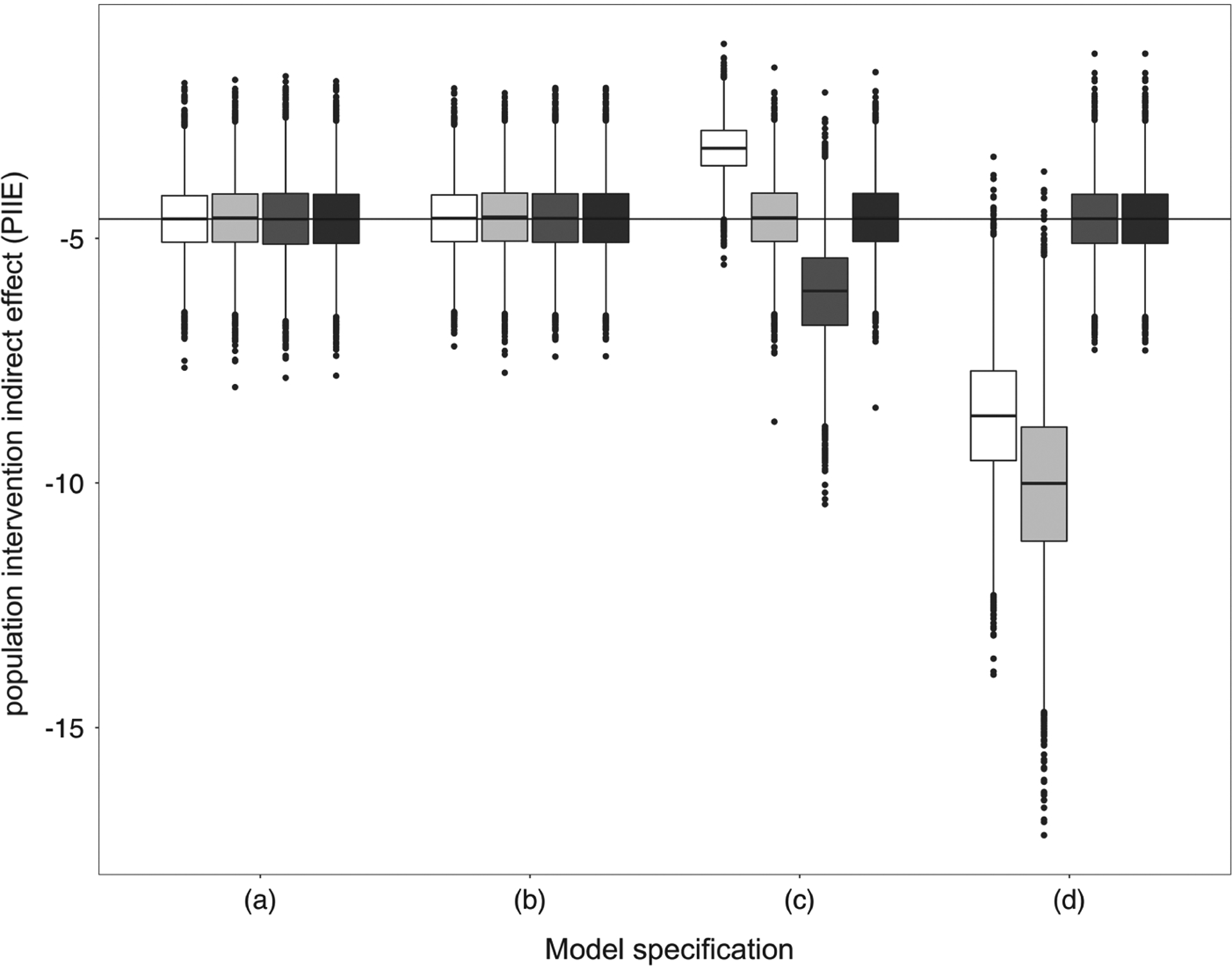
PIIE by estimator and model specifications: , MLE; , semiparametric 1; , semiparametric 2; , semiparametric doubly robust

Table 1.

Operating characteristics by model specification and estimator^†

Estimator	$\widehat{\Psi }$	$\widehat{\text{PIIE}}$	Variance	Proportion bias	0.95 CI coverage
${\mathcal{M}}_{y,z,a}$
MLE	−18.19	−4.61	0.50	< 0.01	0.95
Semiparametric 1	−18.20	−4.59	0.54	< 0.01	0.95
Semiparametric 2	−18.19	−4.61	0.60	< 0.01	0.95
Semiparametric doubly robust	−18.19	−4.61	0.56	< 0.01	0.95
${\mathcal{M}}_{y,z,a}^{\prime }$
MLE	−18.20	−4.59	0.50	< 0.01	0.95
Semiparametric 1	−18.21	−4.57	0.54	< 0.01	0.95
Semiparametric 2	−18.20	−4.59	0.55	< 0.01	0.94
Semiparametric doubly robust	−18.20	−4.59	0.55	< 0.01	0.94
${\mathcal{M}}_z$
MLE	−19.63	−3.17	0.27	−0.31	0.23
Semiparametric 1	−18.22	−4.58	0.54	< 0.01	0.95
Semiparametric 2	−16.70	−6.10	1.04	0.33	0.70
Semiparametric doubly robust	−18.22	−4.58	0.52	< 0.01	0.94
${\mathcal{M}}_{y,a}$
MLE	−14.16	−8.64	1.61	0.88	0.12
Semiparametric 1	−12.75	−10.05	3.32	1.18	0.10
Semiparametric 2	−18.20	−4.60	0.55	< 0.01	0.95
Semiparametric doubly robust	−18.20	−4.60	0.55	< 0.01	0.95

^†For the $\widehat{\Psi }$-column, MLE refers to using the ${\widehat{\Psi }}_{\text{mle}}^{\text{alt}}$-estimator for $\widehat{\text{PIIE}}$. Likewise, semiparametric 1 refers to using ${\widehat{\Psi }}_1$, semiparametric 2 refers to using ${\widehat{\Psi }}_2$ and semiparametric doubly robust refers to using ${\widehat{\Psi }}_{\text{dr}}$.

5. Safer deliveries programme in Zanzibar, Tanzania

The ‘Safer deliveries’ programme aimed to reduce the high rates of maternal and neonatal mortality in Zanzibar, Tanzania, by increasing the number of pregnant women who deliver in a healthcare facility and attend prenatal and postnatal check-ups. At May 2017, the programme was active in six (out of 11) districts in Zanzibar on the islands of Unguja and Pemba. The programme trained community health workers selected by the Ministry of Health to participate in the programme on the basis of their literacy, expressed commitment to the improvement of health and respectability in their communities.

The community health workers worked with community leaders and staff at nearby health facilities to identify and register pregnant women and were expected to visit the woman in her home three times during pregnancy to screen for danger signs and to provide counselling to help the woman to prepare for a facility delivery. During the registration visit, the mobile device application calculated a woman’s risk category (low, medium or high) on the basis of a combination of obstetric and demographic factors. Women categorized as high risk were instructed to deliver at a referral hospital. The application then calculated a recommended savings amount based on the women’s recommended delivery location. On average, high risk women were recommended to save more money than were low or medium risk women as they were recommended to deliver at referral hospitals of which there are only four on the island. This analysis assessed the effectiveness of this tailored savings recommendation by risk category on actual savings.

We considered the high risk category (versus low or medium risk) as our binary exposure of interest, although our methods would equally apply to the categorical exposure variable. The mediator variable was recommended savings in Tanzanian shillings, which was calculated during the first visit. The outcome variable was actual savings achieved by the woman and her family at the time of her delivery. In the analysis, we adjusted for district of residence to account for regional differences in health seeking behaviour and accessibility of health facilities. The PIIE was the best estimand for this research question as we were interested in the mediated effect of savings recommendations under the risk categories that were observed in the current population. Additionally, there was likely to be unmeasured confounding between the exposure (high risk) and outcome (actual savings) relationship because most socio-economic factors and health seeking behaviour that may be associated with other factors related to risk category and a woman’s ability to save were not collected by the programme. Furthermore, confounding of exposure–mediator and mediator–outcome associations was less of a concern as the application calculated the recommended savings on the basis of the delivery location which is determined both by risk category and distance to the appropriate health facility, i.e. women who are in a low risk category are recommended to deliver at the facility that is closest to them, whereas women in the high risk category are recommended to deliver at one of four available referral facilities in Zanzibar.

This study included women who were enrolled in the safer deliveries programme who had a live birth by May 31st, 2017 (n = 4511). We excluded 253 women from the newly added Mkoani district of Pemba Island, two women with missing last menstrual period date and estimated delivery dates, 31 women with invalid enrolment times and 123 women with missing risk category, district or savings information. Our final study population included 4102 women. Therefore, the following analyses are only valid under an assumption that data are missing completely at random. The observed average savings at time of delivery was $14.09. Note that for ease of interpretation we converted from Tanzanian shillings (1 US$ = 2236.60 TSh on May 31st, 2017). We estimated the population intervention indirect effect, i.e. the difference in average savings between the current population of women and a population of women if possibly contrary to the fact every woman had received the savings recommendation of a low or medium risk woman. To estimate the PIIE we employed our four estimators under the following parametric models:

$$\begin{gathered} \text{highrisk}={\alpha }_0+{\alpha }_2^{\text{T}}\text{ district}+{\epsilon }_a, \\ {\text{savings}}_{\text{rec}}={\beta }_0+{\beta }_1\text{ highrisk}+{\beta }_2^{\text{T}}\text{ district}+{\epsilon }_z, \\ {\text{savings}}_{\text{act}}={\theta }_0+{\theta }_1\text{ highrisk}+{\theta }_2{\text{savings}}_{\text{rec}}+{\theta }_3^{\text{T}}\text{ district}+{\epsilon }_y. \end{gathered}$$

Table 2 gives the distribution of variables in this study population. The MLE ${\widehat{\Psi }}_{\text{mle}}^{\text{alt}}$ estimated the average savings for all women if their recommended savings had been set to the amount that they would have been recommended to save if they had not been high risk to be $13.87, resulting in a PIIE of $0.22 with a 95% CI of ($0.15, $0.30) (Table 3). The semiparametric estimator that includes only models for A|C and Y|A, Z, C, ${\widehat{\Psi }}_2$, gave almost identical results. The doubly robust semiparametric estimator of the PIIE was estimated to be $13.95 with a 95% CI of (−$0.03, $0.32). The semiparametric estimator that depends only on a parametric model for Z|A, C, ${\widehat{\Psi }}_1$, resulted in very similar inferences to the doubly robust estimator. To compare these estimators, we conducted a bootstrap test of the null hypothesis that each of the estimators (MLE, semiparametric 1, semiparametric 2) converged to the same probability limit as the semiparametric doubly robust estimator. The procedure was motivated by Hausman (1978) to test directly whether two estimators are consistently estimating the same parameter value. We used 1000 boostrap samples and did not find evidence of a difference between any of the three estimators and the semiparametric doubly robust estimator (P = 0.35 for the MLE; P = 0.14 for the semiparametric 1 estimator; P = 0.36 for the semiparametric 2 estimator). As such, we concluded that there was evidence of a non-zero PIIE—revealing that the tailored savings recommendations to high risk women affects their actual savings by the time of their delivery. On average, if high risk women had been recommended to save what they would have if they were low to medium risk, this would slightly decrease the amount of money that she saved.

Table 2.

Characteristics of the safer deliveries study population (n=4102)

Variable	n (%)
Risk category
Low or medium	3364 (82)
High	738 (18)
District
North A	977 (24)
North B	1392 (34)
Central	691 (17)
West	798 (19)
South	244 (6)
Recommended savings ($)
Mean (standard deviation)	13.12 (6.03)
Actual savings
Mean (standard deviation)	14.09 (12.11)

Table 3.

Effect of risk category on actual savings mediated by recommended savings (n=4102)

Estimator	$\widehat{\Psi }$	$\widehat{\text{PIIE}}$	Standard error	95% CI
MLE	13.87	0.22	0.04	(0.15, 0.30)
Semiparametric 1	14.08	0.02	0.11	(−0.20, 0.23)
Semiparametric 2	13.87	0.22	0.05	(0.13, 0.31)
Semiparametric doubly robust	13.95	0.14	0.09	(−0.03, 0.32)

6. Discussion

In this paper, we have presented a decomposition of the PIE, which we have argued is useful to address policy-related questions at the population level especially in the presence of a harmful exposure. In addition, the decomposition offers an alternative to the recently proposed decompositions for the ETT (Vansteelandt and VanderWeele, 2012) and the attributable fraction (Sjölander, 2018). Importantly, our resulting PIIE is robust to unmeasured confounding of the exposure–outcome relationship, which does not hold for the NIE, NIE on the exposed or the natural indirect attributable fraction. We note that, elsewhere, we recently established that the NIE can in fact be identified if one replaces assumption 4 with the assumption that there is no additive interaction between the mediator and the unmeasured confounder of the A–Y-association, which is a strictly stronger requirement than that for the PIIE (Fulcher et al., 2019).

We developed a doubly robust estimator for the PIIE, which is consistent and asymptotically normal in a union model where at least one of the following conditions holds:

1. the outcome and exposure models are correctly specified or

2. the mediator model is correctly specified.

Our estimator is strictly more robust than the multiply robust estimator for the NIE that was proposed by Tchetgen Tchetgen and Shpitser (2012), which requires that any two of the three models are correctly specified. Sjölander (2018) proposed a doubly robust estimator for the natural indirect attributable fraction requiring that either p(Y|A, Z, C) or p(A|Z, C) is correctly specified and either p(Y|A, C) or p(A|C) is correctly specified. As mentioned by Sjölander (2018), a doubly robust estimator may not be realizable because various submodels of the union models are not variation independent, such that misspecification of the former generally rules out the possibility that the latter could still be correctly specified. For example, when Z is binary, a logistic model for p(Y|A, Z, C) would imply a complex form for p(Y|A, C). In a separate strand of work, Lendle et al. (2013) developed an estimator for the NIE among the (un)exposed with the same robustness properties as in Sjölander (2018).

We emphasize that the use of the doubly robust estimator of the PIIE does not obviate concerns about unmeasured confounding of the exposure–mediator or mediator–outcome relationship, or exposure-induced mediator–outcome confounding. When such confounding is of concern, a sensitivity analysis should be performed (VanderWeele and Arah, 2011; Tchetgen Tchetgen and Shpitser, 2012, 2014). Investigators should exercise caution if they wish to report the PIDE and PIE also, as these effects are not robust to exposure–outcome confounding. If exposure–outcome unmeasured confounding can be ruled out with reasonable certainty, then one can estimate the PIDE by using our doubly robust estimator for Ψ and the well-known doubly robust estimator for E{Y(a*)} from Robins et al. (2000). Likewise, the PIE can be estimated by using the doubly robust estimator that was developed by Hubbard and Van der Laan (2008).

Lastly, although the front door criterion has been available in the literature for several years, this is the first methodology developed for semiparametric estimation and inference of the front door functional Ψ. Therefore, when an investigator believes that she has identified one or more mediator variables that satisfy the front door criterion, she can use our proposed methodology to obtain an estimate of the PIE or the ACE that is not only doubly robust, but also robust to unmeasured confounding of the exposure–outcome relationship.

7. Description of data sets and programs

The frontdoorpiie R package is available to download from https://isabelfulcher.github.io/frontdoorpiie/.

The R code for the simulation study is available from https://github.com/isabelfulcher/frontdoorpiie_sim/.

The safer deliveries programme data are available from the authors on reasonable request and with permission of D-tree International and the Zanzibar Ministry of Health. Researchers who are interested in using the safer deliveries data should submit a request to Isabel Fulcher (isabel_fulcher@hms.harvard.edu) to initiate the process.

References

- Angrist JD, Imbens GW and Rubin DB (1996) Identification of causal effects using instrumental variables. J. Am. Statist. Ass, 91, 444–455. [Google Scholar]
- Avin C, Shpitser I and Pearl J (2005) Identifiability of path-specific effects. Department of Statistics, University of California at Los Angeles, Los Angeles. [Google Scholar]
- Bickel PJ, Klaassen CA, Ritov Y and Wellner JA (1998) Efficient and Adaptive Estimation for Semiparametric Models, vol. 2 New York: Springer. [Google Scholar]
- Campbell DT and Stanley JC (1963) Experimental and Quasi-experimental Designs for Research. Boston: Houghton Mifflin. [Google Scholar]
- Casella G and Berger RL (2002) Statistical Inference, vol. 2 Pacific Grove: Duxbury. [Google Scholar]
- Chernozhukov V, Chetverikov D, Demirer M, Duflo E, Hansen C, Newey W and Robins J (2017) Double/debiased machine learning for treatment and structural parameters. Econmetr. J, 21, C1–C68. [Google Scholar]
- Fulcher I (2017) frontdoorpiie. Department of Biostatistics, Harvard T.H. Chan School of Public Health, Boston: (Available from https://github.com/isabelfulcher/frontdoorpiie.) [Google Scholar]
- Fulcher IR, Shi X and Tchetgen Tchetgen EJ (2019) Estimation of natural indirect effects robust to unmeasured confounding and mediator measurement error. Epidemiology, 30, 825–834. [DOI] [PMC free article] [PubMed] [Google Scholar]
- Geneletti S and Dawid AP (2011) Defining and identifying the effect of treatment on the treated In Causality in the Sciences (eds Illari PMI, Russo F and Williamson J), ch. 34 Oxford: Oxford University Press. [Google Scholar]
- Greenland S and Drescher K (1993) Maximum likelihood estimation of the attributable fraction from logistic models. Biometrics, 49, 865–872. [PubMed] [Google Scholar]
- Hahn J (1998) On the role of the propensity score in efficient semiparametric estimation of average treatment effects. Econometrica, 66, 315–331. [Google Scholar]
- Hausman JA (1978) Specification tests in econometrics. Econometrica, 46, 1251–1271. [Google Scholar]
- Hubbard AE and Van der Laan MJ (2008) Population intervention models in causal inference. Biometrika, 95, 35–47. [DOI] [PMC free article] [PubMed] [Google Scholar]
- Imai K, Keele L and Tingley D (2010a) A general approach to causal mediation analysis. Psychol. Meth, 15, 309–334. [DOI] [PubMed] [Google Scholar]
- Imai K, Keele L and Yamamoto T (2010b) Identification, inference and sensitivity analysis for causal mediation effects. Statist. Sci, 25, 51–71. [Google Scholar]
- Imbens GW and Lemieux T (2008) Regression discontinuity designs: a guide to practice. J. Econmetr, 142, 615–635. [Google Scholar]
- Lendle SD, Subbaraman MS and van der Laan MJ (2013) Identification and efficient estimation of the natural direct effect among the untreated. Biometrics, 69, 310–317. [DOI] [PMC free article] [PubMed] [Google Scholar]
- Lipsitch M, Tchetgen Tchetgen E and Cohen T (2010) Negative controls: a tool for detecting confounding and bias in observational studies. Epidemiology, 21, 383–388. [DOI] [PMC free article] [PubMed] [Google Scholar]
- Miao W and Tchetgen Tchetgen E (2017) Invited commentary: bias attenuation and identification of causal effects with multiple negative controls. Am. J. Epidem, 185, 950–953. [DOI] [PMC free article] [PubMed] [Google Scholar]
- Newey WK (1990) Semiparametric efficiency bounds. J. Appl. Econmetr, 5, 99–135. [Google Scholar]
- Newey WK and Robins JM (2018) Cross-fitting and fast remainder rates for semiparametric estimation. Preprint arXiv:1801.09138. [Google Scholar]
- Pearl J (2001) Direct and indirect effects In Proc. 17th Conf. Uncertainty in Artificial Intelligence (eds Breese J and Koller D), pp. 411–420. San Francisco: Morgan Kaufmann. [Google Scholar]
- Pearl J (2009) Causality. Cambridge: Cambridge University Press. [Google Scholar]
- Pearl J (2012) The causal mediation formula—a guide to the assessment of pathways and mechanisms. Prevn Sci, 13, 426–436. [DOI] [PubMed] [Google Scholar]
- Robins J (1986) A new approach to causal inference in mortality studies with a sustained exposure period—application to control of the healthy worker survivor effect. Math. Modllng, 7, 1393–1512. [Google Scholar]
- Robins J, Li L, Mukherjee R, Tchetgen Tchetgen E and van der Vaart A (2017) Higher order estimating equations for high-dimensional models. Ann. Statist, 45, 1951–1987. [DOI] [PMC free article] [PubMed] [Google Scholar]
- Robins JM, Rotnitzky A and Scharfstein DO (2000) Sensitivity analysis for selection bias and unmeasured confounding in missing data and causal inference models In Statistical Modelsin Epidemiology, the Environment, and Clinical Trials (eds Halloran E and Berry D), pp. 1–94. New York: Springer. [Google Scholar]
- Shpitser I (2013) Counterfactual graphical models for longitudinal mediation analysis with unobserved confounding. Cogn. Sci, 37, 1011–1035. [DOI] [PubMed] [Google Scholar]
- Sjölander A (2018) Mediation analysis with attributable fractions. Epidem. Meth, 7, no. 1. [Google Scholar]
- Sjölander A and Vansteelandt S (2010) Doubly robust estimation of attributable fractions. Biostatistics, 12, 112–121. [DOI] [PubMed] [Google Scholar]
- Tchetgen Tchetgen EJ and Shpitser I (2012) Semiparametric theory for causal mediation analysis: efficiency bounds, multiple robustness, and sensitivity analysis. Ann. Statist, 40, 1816–1845. [DOI] [PMC free article] [PubMed] [Google Scholar]
- Tchetgen Tchetgen EJ and Shpitser I (2014) Estimation of a semiparametric natural direct effect model incorporating baseline covariates. Biometrika, 101, 849–864. [DOI] [PMC free article] [PubMed] [Google Scholar]
- Van der Laan MJ and Rose S (2011) Targeted Learning: Causal Inference for Observational and Experimental Data. New York: Springer Science and Business Media. [Google Scholar]
- VanderWeele TJ and Arah OA (2011) Bias formulas for sensitivity analysis of unmeasured confounding for general outcomes, treatments, and confounders. Epidemiology, 22, 42–52. [DOI] [PMC free article] [PubMed] [Google Scholar]
- Vansteelandt S and VanderWeele TJ (2012) Natural direct and indirect effects on the exposed: effect decomposition under weaker assumptions. Biometrics, 68, 1019–1027. [DOI] [PMC free article] [PubMed] [Google Scholar]
Associated Data
This section collects any data citations, data availability statements, or supplementary materials included in this article.