Bayesian Probabilistic Analysis of DEER Spectroscopy Data Using Parametric Distance Distribution Models

Abstract

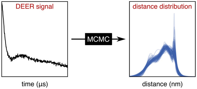
Double Electron–Electron Resonance (DEER) spectroscopy measures distance distributions between spin labels in proteins, yielding important structural and energetic information about conformational landscapes. Analysis of an experimental DEER signal in terms of a distance distribution is a nontrivial task due to the ill-posed nature of the underlying mathematical inversion problem. This work introduces a Bayesian probabilistic inference approach to analyze DEER data, using a multi-Gauss mixture model for the distance distribution. The method uses Markov Chain Monte Carlo (MCMC) sampling to determine a posterior probability distribution over model parameter space. This distribution contains all the information available from the data, including a full quantification of the uncertainty about the parameters. The corresponding uncertainty about the distance distribution is captured via an ensemble of posterior predictive distributions. Several synthetic examples illustrate the method. An experimental example shows the importance of model checking and comparison using residual analysis and Bayes factors. Overall, the Bayesian approach allows for more robust inference about protein conformations from DEER spectroscopy.

Graphical Abstract

1. Introduction

Double Electron–Electron Resonance (DEER) spectroscopy is a pulse Electron Paramagnetic Resonance (EPR) technique utilized for determining distances between spin centers on a nanometer scale,^1,2 often on proteins. DEER resolves the full distribution of distances in an ensemble of proteins, making it possible to directly quantify conformational landscapes.^3–5 DEER measures an oscillatory time-domain signal that depends on the magnitude of the magnetic dipole–dipole interactions between the spin centers. In the analysis, this signal is fitted with a model that includes a distance distribution. Mathematically, this constitutes an ill-posed inversion problem. Assessment of uncertainty in the fitted distance distribution is therefore challenging, but is crucial for making sound conclusions about the conformational landscape.

Analysis approaches for obtaining a distance distribution range from analytical solutions⁶ to deep neural networks.⁷ Two methods based on least-squares fitting have seen the widest practical application: Tikhonov regularization and Gaussian mixture models.^8–14 Tikhonov regularization utilizes a non-parametric distance distribution model and includes a roughness penalty for the distribution into the fitting objective function. Gaussian mixture models are parametric and represent the distribution as a linear combination of a few Gaussian functions. Both Tikhonov regularization and Gaussian models can be fit directly to the raw data in a single fitting step.¹⁵ In both approaches, however, correctly quantifying and visualizing uncertainty is challenging.

For Tikhonov regularization, partial uncertainty analysis is commonly conducted by manually varying some parameters in the analysis (background, modulation depth, noise) and summarizing the sensitivity of the extracted distance distribution to these parameters into error bands around the fitted distribution.¹⁰ Another partial approach is based on Bayesian inference and quantifies the uncertainty in the distribution due to the noise in the signal.¹⁶ Unfortunately, as currently implemented, this requires a priori background correction and cannot incorporate parameters beyond noise.

For Gaussian mixture models, uncertainty analysis relies primarily on parameter confidence intervals, which are obtained from the covariance matrix or by explicitly exploring the sensitivity of the objective function on the parameter values.^11–13,17 The parameter confidence intervals are then propagated to the distance domain to yield error bars on the distribution. This method assumes that the error surface is quadratic and that the parameters are unbounded, neither of which is generally true.

Another method to obtain confidence intervals for both approaches is bootstrapping, which generates an ensemble of distributions by analyzing a large number of synthetically generated hypothetical signals based on the fitted model.¹⁵

Here, we present a Bayesian probabilistic inference approach^18–20 to analyze DEER data using a multi-Gauss mixture model. The method models and analyses the raw DEER data directly and yields a full posterior probability distribution over all model parameters, providing complete quantitative information about uncertainty and correlations for all parameters, without any limiting assumptions. We also introduce distribution ensembles to more correctly represent uncertainty about the distance distribution, including correlations which are neglected when using visualizations based on error bands.

The paper is structured as follows. Section 2 presents the model used to describe the DEER signal. Section 3 introduces the Bayesian inference approach. Section 4 applies this method to a simple distribution while more realistic distributions are evaluated in Section 5. Section 6 applies the method to experimental data, including model checking and comparison. The final section provides conclusions regarding the method.

2. DEER theory

We base our analysis on the standard model for 3- and 4-pulse DEER.¹ In this model, the noise-free DEER signal is

$$V_M\left(t\right)=V_0\cdot V_{\text{intra }}\left(t\right)\cdot V_{\text{inter }}\left(t\right)$$ (1)

where t is the position of the pump pulse and V₀ is the echo amplitude in the absence of the pump pulse.

V_intra(t) is the intra-molecular modulation function and is given by

$$V_{\text{intra }}\left(t\right)=\left(1-\mathrm{\lambda }\right)+\mathrm{\lambda }{\int }_0^{\infty }K\left(t,r\right)P\left(r\right)\text{d}r$$ (2)

with the modulation depth λ (satisfying 0 < λ ≤ 1) and the normalized distribution P(r) of the spin–spin distance r (satisfying P(r) ≥ 0 and ${\int }_0^{\infty }P\left(r\right)\text{d}r=1)$. K(t, r)is the dipolar kernel function, given by

$$K\left(t,r\right)={\int }_0^1\text{cos}\left(\left(1-3z^2\right)D{r}^{-3}t\right)\text{d}z$$ (3)

with the constant $D=\left({\mu }_0/4\pi \right){\left(g_{\text{e}}{\mu }_{\text{B}}\right)}^2/\hslash$. In our implementation, the integral in Eq. (2) is numerically evaluated over the range 1nm ≤ r ≤ 10nm.

V_inter(t) is the inter-molecular modulation function, also called the background. In this work, we use

$$V_{\text{inter }}\left(t\right)=\text{exp}\left(-k\left|t\right|\right)$$ (4)

Here, k is the decay rate constant $k=\left(8{\pi }^2/9\sqrt{3}\right)Dc\lambda$, with the spin concentration c (in spins/m³) and the modulation depth λ.

We represent the spin–spin distance distribution P(r) used in Eq. (2) as a linear combination of normalized Gaussian basis functions

$$P\left(r\right)=\sum _{i=1}^m{A}_i\text{Gauss}\left(r;r_{0,i},w_i\right)$$ (5)

where m is the number of Gaussians, A_i are the amplitudes (with ${\sum }_i{A}_i=1$), r_0,i are the centers of the Gaussians, and w_i are the full widths at half maximum. In the statistical literature, this is called a Gaussian mixture model.

In practice, the echo amplitude is measured at a set of discrete pump pulse positions t_i up to a maximum t_max, so that the experimental signal consists of a vector V with elements V_i = V(t_i). In addition, the experimental signal is corrupted by measurement noise. This noise is approximately Gaussian, uncorrelated, and of constant variance σ².¹⁶ We can thus write each measured data point as a random sample from a Gaussian (normal) distribution

$$V_i~\text{Normal}\left(V_M\left(t_i\right),{\sigma }^2\right)$$ (6)

where ~ indicates that the quantity on the left is a random sample from the distribution on the right. In vector form, the full signal is modeled as a random sample from a multidimensional Gaussian with center V_M and isotropic covariance matrix σ²I

$$V~\text{Normal}\left(V_M,{\sigma }^{2}I\right)$$ (7)

where I is the identity matrix.

The full set of parameters for this multi-Gauss DEER model includes the distribution parameters r_0,i, w_i, and A_i, the time-domain parameters k, λ, and V₀, and the noise standard deviation σ. We collect them into a parameter vector

$$\theta =\left(\left\{r_{0,i}\right\},\left\{w_i\right\},\left\{A_i\right\},k,\lambda ,V_0,\sigma \right)$$ (8)

Thus, the model has N = 6, 10, 13, and 16 parameters for a one-, two-, three-, and four-Gauss distribution, respectively. This number is much smaller than the typical number of experimental data points, which can be several hundred.

Figure 1 illustrates the important quantities in this model, as well as the parameters. Figure 1A shows a synthetic distance distribution (black) that is close to Gaussian in shape and a one-Gaussian fit to it (red) while Fig. 1B shows the noise-free and a noisy time-domain signal derived from the synthetic distance distribution.

Figure 1:

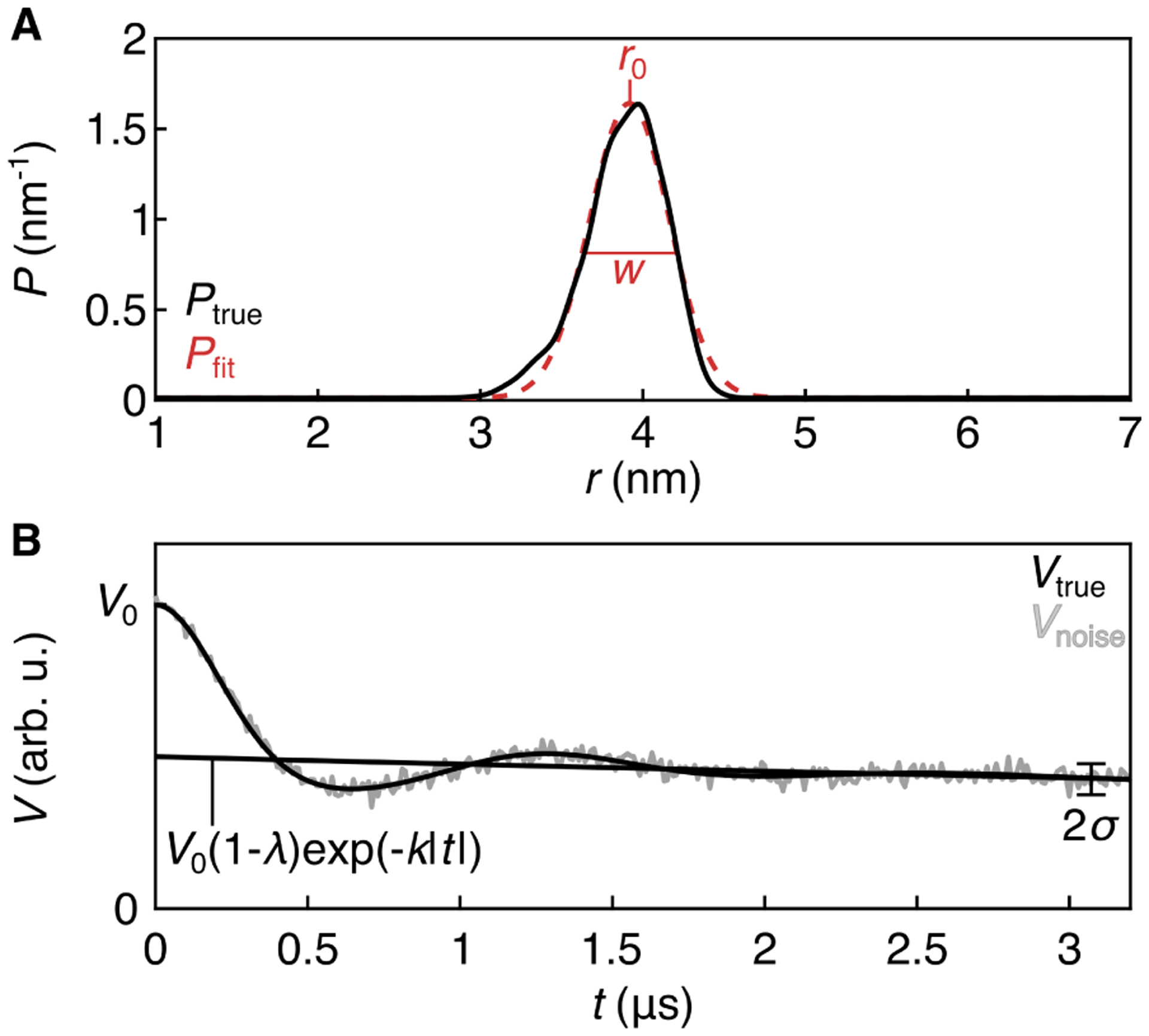
Quantities and parameter in the standard DEER model. A: P_true (black) is distribution 3992 from the synthetic T4L test set,¹⁴ and P_fit is a one-Gaussian fit to P_true, with parameters r₀ and w indicated. B: Noise-less trace derived from P_true (black) and overlaid with noise (gray). Time-domain parameters k, λ, V₀, and σ are indicated.

3. Bayesian inference

The goal of analyzing DEER data within the above model M is to estimate the N model parameters θ from the measured signal V and any additional information I that is included, and then to transfer the inferences about θ to inferences about the distance distribution P(r). The most complete information obtainable about the parameters is the probability distribution of θ, conditioned on the given V, M, and I. This is denoted as

$$p\left(\theta \mid V,M,I\right)$$ (9)

and is called the posterior probability distribution, or simply posterior. It is a probability density defined over the entire N-dimensional 239 parameter space and quantifies how probable any set of parameters is. It represents the complete information that can be inferred about the parameters of the assumed model M from the included evidence (V and I). Regions in parameter space with high posterior density reveal probable sets of parameters, and the spread of the distribution quantifies the uncertainty. The posterior distribution also reveals all correlations between parameters.

To calculate the posterior, we utilize Bayes’ theorem, which in its full form is^18–21

$$p\left(\theta \mid V,M,I\right)=\frac{p(V\mid \theta ,M,I)p(\theta \mid M,I)}{p(V\mid M,I)}$$ (10)

The denominator, p(V |M, I), represents the probability of a signal given the proposed model, integrated over all possible parameter values. Since it is independent of θ, it does not affect the shape of the posterior. Therefore, we can neglect it and use

$$p\left(\theta \mid V,M,I\right)\propto p\left(V\mid \theta ,M,I\right)\cdot p\left(\theta \mid M,I\right)$$ (11)

The first term on the right-hand side, p(V |θ, M, I), is called the likelihood and defines the probability of a signal given a parameter set, model choice, and additional information. In our case with normally distributed errors as given in Eq. (7), we use the multidimensional Gaussian

$$p\left(\theta \mid V,M,I\right)=\text{Normal}\left(V;V_M\left(\theta \right),{\sigma }^{2}I\right)\propto \text{exp}\left(-\frac{V-V_M{\left(\theta \right)}^2}{2{\sigma }^2}\right)$$ (12)

with center V_M and covariance matrix σ²I. This distribution quantifies the degree of fit between the data and the model. (Its negative logarithm is minimized in least-squares fitting.)

The second factor on the right-hand side in Eq. (11), p(θ|M, I), is called the prior probability distribution, or simply prior. It represents information about the parameters prior to taking the observed data V into account. If information about individual parameters θ_i is not correlated, the prior factors into a product

$$p\left(\theta \mid M,I\right)=\prod _{i}p\left({\theta }_i\mid M,I\right)$$ (13)

We specify priors for all parameters in the next subsection.

3.1. Priors

To calculate the posterior from Eq. (11), both a likelihood and a full prior distribution must be specified. It is essential to define the prior such that it appropriately captures prior information, I, about the parameters but is diffuse enough to not introduce unwarranted bias into the analysis. In the following, we describe our choices of priors for all model parameters. The priors are shown on the left-hand side of Fig. 2.

Figure 2:

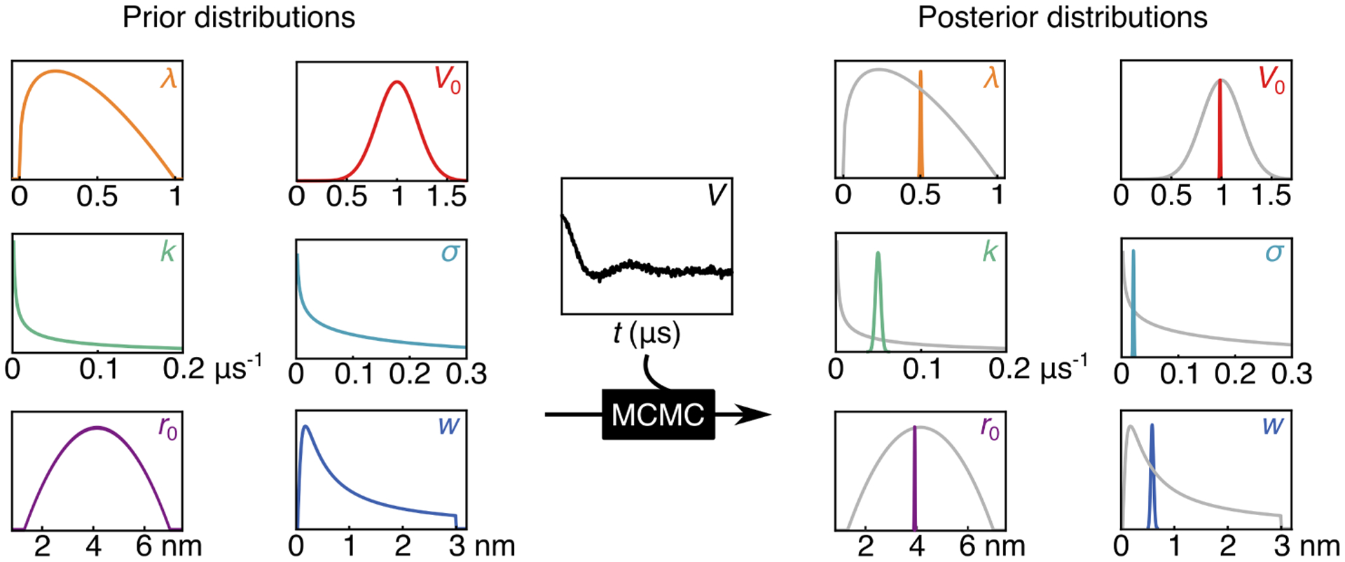
Visualization of the Bayes process. The priors for all parameters (modulation depth (λ), echo amplitude (V₀), background decay constant (k), noise (σ), Gaussian center (r₀), and Gaussian width (w)) and the raw data are input into the ‘black box’ process of MCMC and the output is the marginalized posterior distribution for each parameter. The marginalized posteriors represent a probability distribution of possible values for each parameter. Distribution 3992 from the synthetic T4L test set was used as the true distribution from which parameters were derived.¹⁴

Modulation depth λ.

The minimal information about λ is that it lies somewhere between 0 and 1, irrespective of the sample and the spectrometer. The associated prior can be represented as a uniform distribution

$$p\left(\lambda \mid M,I\right)=\text{Uniform}\left(\lambda ;0,1\right)$$ (14)

with lower bound 0 and upper bound 1. If additional information about the spectrum (e.g. nitroxide at Q-band) and the excitation profile of the pump pulse (e.g. a 10 ns π pulse) is available, the modulation depth can be estimated. Then, a more focused probability distribution can be constructed that is centered at this estimated value and has sufficient spread to capture uncertainty in the information. We use a beta distribution

$$p\left(\lambda \mid M,I\right)=\text{Beta}\left(\lambda ;1.3,2\right)$$ (15)

where the two arguments are shape parameters. For our test cases, the choice of prior made no difference on the obtained posterior distributions. This indicates that the data itself contained strong information about λ.

Echo amplitude V₀.

Before analysis, we rescale the signal, V = V /max(V). Therefore, for the rescaled signal, we know V₀ has a positive value near 1. We capture this information with a normal distribution bounded above zero with a standard deviation of 0.2

$$p\left(V_0\mid M,I\right)=\text{Bnd}\left(\text{Normal}\left(V_0;1,{0.2}^2\right),0\right)$$ (16)

Background decay rate k.

As prior for k, we use the gamma distribution (which ensures k is non-negative)

$$p\left(k\mid M,I\right)=\text{Gamma}\left(k;0.5,2\mathrm{\mu }{\text{s}}^{-1}\right)$$ (17)

where the two arguments are the shape and the rate parameter, respectively. This distribution has significant density for k < 0.1μs⁻¹, corresponding to λc < 0.1mM. If the spin concentration is known, a tighter prior can be formulated.

Noise level σ.

Without taking the data into account, an appropriate prior on the noise standard deviation for the rescaled signal is one which skews heavily towards zero and diminishes towards 1. We choose a gamma distribution

$$p\left(\sigma \mid M,I\right)=\text{Gamma}\left(\sigma ;0.7,2\right)$$ (18)

Gaussian centers r_0,i.

We choose a prior with significant density around the most common distances (2–6 nm) and diminished probability outside, using a beta distribution

$$p\left(r_{0,i}\mid M,I\right)\propto \text{Beta}\left(\frac{r_{0,i}-r_{\text{min}}}{r_{\text{max}}-r_{\text{min}}};2,2\right)$$ (19)

where r_min and r_max are 1.3 and 7 nm, respectively, and we disregard the normalization factor 1/(r_max − r_min).

Gaussian widths w_i.

Based upon general knowledge of spin–spin distance distributions, we choose the prior to skew towards values below 1 nm but with substantial probability at larger widths. A bounded inverse gamma distribution captures the desired shape

$$p\left(w_i\mid M,I\right)=\text{Bnd}\left(\text{InvGamma}\left(w_i;0.1,0.2\text{nm}\right),0.05\text{nm},3\text{nm}\right)$$ (20)

The distribution is truncated between 0.05 and 3 nm, since it is very unlikely to have distributions with widths beyond these bounds. If a sample is analyzed where these assumptions are possibly not satisfied, the prior can be adjusted.

Gaussian amplitudes A_i.

Since we have no prior information on A_i, we use a flat m-dimensional Dirichlet distribution

$$p\left(A_1,\dots ,A_m\mid M,I\right)=\text{Dirichlet}\left(1_m\right)$$ (21)

where 1_m is the m-dimensional vector of ones. The Dirichlet distribution automatically satisfies 0 ≤ A_i ≤ 1 and ${\sum }_{i=1}^m{A}_i=1$.

3.2. MCMC sampling

Although the posterior is now formulated explicitly via Eqs. (11), (12), (13), and all the individual prior distributions, it is a multidimensional distribution so complicated that the integrals necessary to determine its mean and other statistics are impossible to evaluate analytically. Therefore, numerical Markov Chain Monte Carlo (MCMC) sampling methods are used to generate a representation of the posterior in terms of a set of samples in the N-dimensional parameter space. An MCMC sampler generates a chain of samples from the posterior, where each sample depends on the previous one. Once converged, the chain samples represent the posterior. Using this representation, calculating the above statistics and other analysis is straightforward.

In our previous work on Bayesian analysis, we used the Gibbs sampler.¹⁶ This sampler requires specific forms of the priors and is very inefficient in high-dimensional parameter spaces. In this work, we use the No-U-Turn Sampler (NUTS),²² a very efficient and self-tuning Hamiltonian Monte Carlo (HMC) sampler,²³ as implemented in the Python-based probabilistic programming package PyMC3, version 3.8.²⁴ All MCMC simulations were run on standard laptop computers. The Python code that implements the DEER model and the MCMC sampling can be found at https://github.com/StollLab/dive.

We use NUTS to generate 5–8 independent MCMC chains. The chains are initialized with different starting points that are randomly sampled from the prior distribution. These points are then propagated for 5,000 steps to tune the sampler. The tuning steps are discarded. The chains are then propagated for 20,000–80,000 steps to generate a large number of posterior samples. The exact sampler settings are noted in the figure captions. The chains are long enough to provide convergence, as assessed via the rank-normalized split $\widehat{R}$ statistic.^25–27 $\widehat{R}$ is calculated for each parameter separately and compares the between-chains and within-chain variances to determine whether the chains have reached equilibrium for that parameter (corresponding to $\widehat{R}\approx 1$) or not $\left(\widehat{R}>1\right)$. In our approach, sampling was continued until $\widehat{R}<1.01$ for all parameters.

When using MCMC sampling with mixture models such as Eq. (5), one encounters a phenomenon known as label switching. For example, switching the labels of the two Gaussians in a two-Gauss distance distribution changes the location in parameter space (θ₁ ≠ θ₂), but does not affect the distance distribution (P(θ₁) = P(θ₂)) nor the likelihood or the posterior. This renders the posterior multi-modal, complicating both the sampling and the analysis of the posterior. Different approaches exist to prevent label switching.^28,29 In this work, we take an approach similar to on-line relabeling²⁸ and enforce the constraints r_0,1 ≤ r_0,2 ≤·…·≤ r_0,m after every sample to restrict the parameter space.²⁹ This technique worked well in most cases that we encountered, and typically provided clean uni-modal marginalized posteriors. Occasionally, due to the imposed constraints, chains get stuck in regions with r_0,i ≈ r_0,j, corresponding to the coalescence of two basis functions. Such chains are easily identified via how they degrade $\widehat{R}$ and are removed before further analysis.

3.3. Posterior analysis

After convergence, the pooled samples from all chains represent the full N-dimensional posterior p(θ|V,M, I). Due to its large dimensionality, it is not possible to visualize it directly. Instead we examine each parameter individually using a marginalized posterior, which is obtained by integrating the full posterior over all other parameters. This integral is approximated by generating a histogram of the parameter values from all samples and conducting a kernel density estimation of the histogram, smoothed with a Gaussian with a line width of 1/5 of the standard deviation of the parameter values. This results in a one-dimensional distribution that can easily be plotted and summarized in terms of the mean, mode, and spread. On the right of Fig. 2, the marginalized posteriors are shown in color, together with the priors in gray. In this case, they are much narrower than the corresponding priors. The spread of the posterior distribution is both a qualitative and quantitative measure of inferential uncertainty.

However, marginalization discards all information about correlation between parameters. As will be shown, many of the parameters in our model are correlated. Therefore, we also display and examine two-dimensional marginalized posteriors between pairs of parameters (see Sec. 4).

Finally, we will additionally visualize the results of the Bayesian inference in terms of a small set of posterior predictive samples of the noise-free signal, V_M(θ⁽ⁱ⁾), and the distance distribution, P(θ⁽ⁱ⁾). Here, θ⁽ⁱ⁾ represent a random sample from the pooled MCMC samples, with i indicating the associated chain sample index.

4. Basic illustration

In this and the next section, we illustrate the probabilistic analysis method on several synthetic distributions of increasing complexity. All of the synthetic data are based on distributions taken from the large simulated T4 lysozyme (T4L) test data set published by Edwards and Stoll in 2018.^14,30 The distributions in this test data set were generated computationally from an in silico spin-labeled crystal structure of T4L. The indices of the chosen distributions are given in the figure captions. We take the distributions from the test data set as ground truth.

Figures 3 and 4 show the first example. It uses the distance distribution from Fig. 1A that resembles a single Gaussian. Two noisy signal traces generated from this distance distribution are shown in Fig. 4A. The trace indicated as V_good(t) (blue) has favorable values for the modulation depth, background decay rate, trace length, and noise level (λ = 0.5, k = 0.05 μs⁻¹, t_max = 3.2 μs, σ = 0.02). Comparatively, the trace V_poor(t) (green) has less ideal values for all of these parameters (λ = 0.2, k = 0.2 μs⁻¹, t_max = 1.6 μs, σ = 0.05), providing a challenging case with higher uncertainty.

Figure 3:

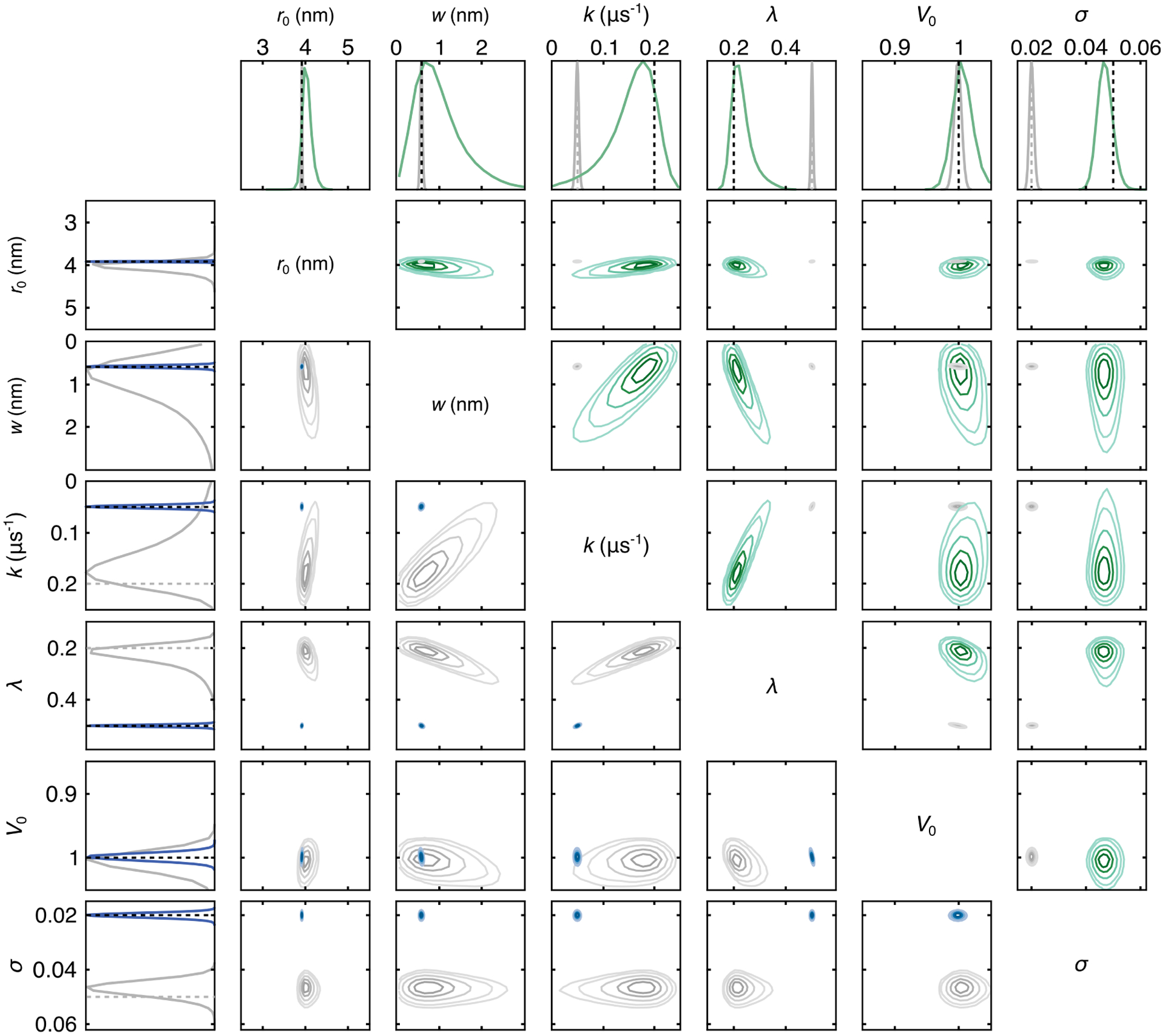
Plots of the marginalized parameters posteriors of the two single-Gauss test cases and all pairwise correlations between parameters. The results for the poor test case are indicated in green and those for the good test case are in blue. The dotted lines reference the true parameter values. Both cases are shown in every subplot for comparison. The top row and upper triangle show the poor test case results (green), and the first column and lower triangle show the good test case results (blue). Both test cases are generated from distribution 3992 from the Edwards/Stoll test set. Contour levels are at 0.05, 0.1, 0.25, 0.5, and 0.75 of the maximum of the distribution. The MCMC simulation was run with 5 chains with 20,000 posterior samples each.

Figure 4:

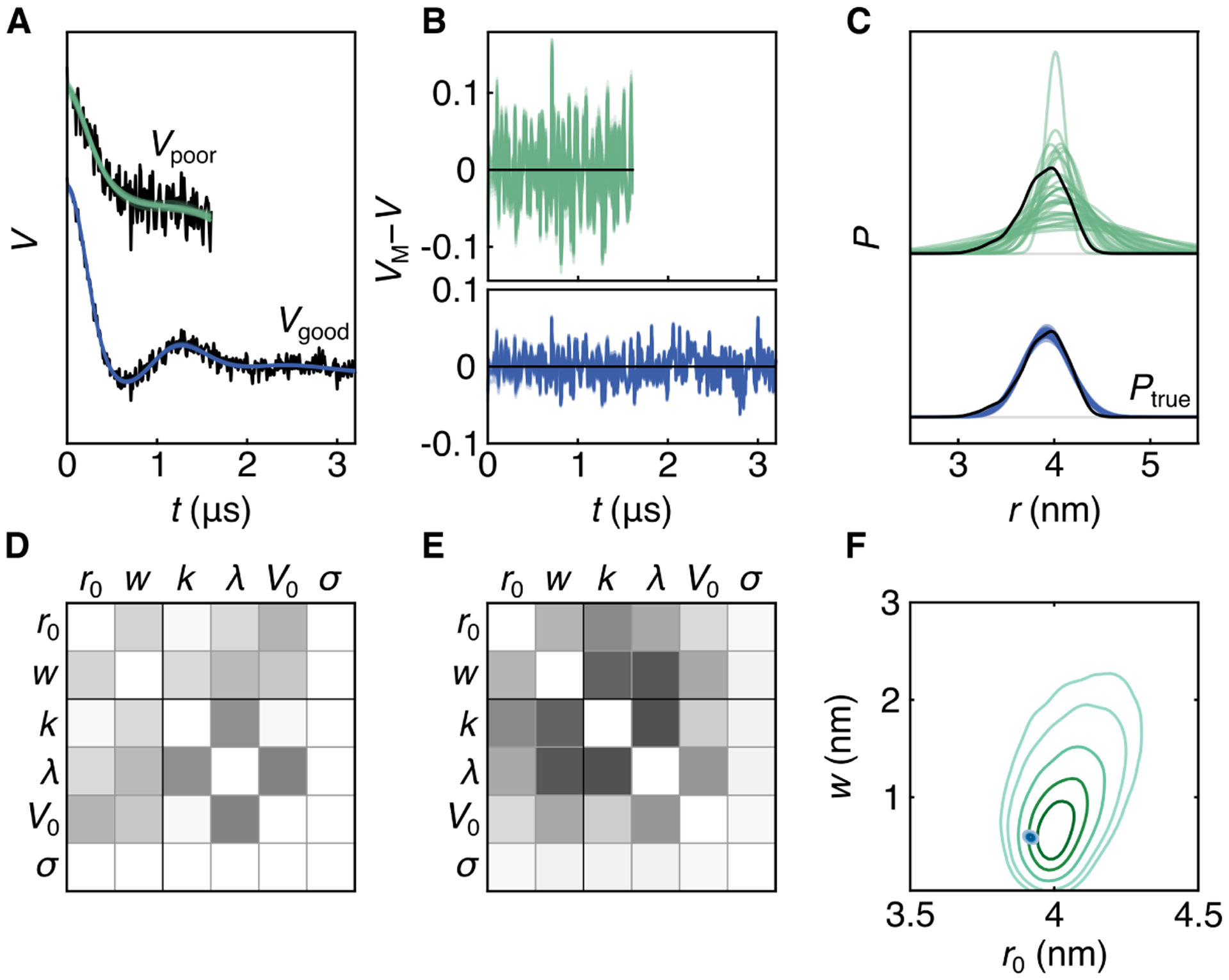
Bayesian inference with a single-Gauss distribution model. A: The two data realizations (black) overlaid with the fits predicted from an ensemble of 30 MCMC samples (color). B: Residuals for both traces for all 30 samples (color). C: Ensemble of 30 distributions (color) from MCMC samples plotted with P_true (black), distribution 3992 from the synthetic T4L test set.¹⁴ D: Correlation matrix of all parameters for the good trace, white indicating no correlation and black indicating full correlation. E: Correlation matrix of all parameters for the poor trace. F: 2D marginalized posteriors for Gaussian width and center for both cases.

Figure 3 summarizes the results of the Bayesian analysis for both cases. The top row shows the marginalized posteriors for each parameter for the poor case (green) while the first column shows the same for the good case (blue). Both cases are shown on all plots, one of them grayed out. The dashed lines for r₀ and w indicate values obtained by directly fitting a Gaussian to the synthetic distribution, and for the other parameters they indicate the values used in generating the signal. For the longer and less noisy trace, the ground-truth parameters are recovered accurately, and there is very little uncertainty about the inferred parameters, as represented by the narrowness of the distributions. The analysis of the shorter and noisier trace yields posterior modes of each parameter near the expected values. The distributions, however, are much broader, reflecting the detrimental effect of the larger noise level and shorter trace length. The distributions are asymmetric, particularly for w, k, and λ.

The rest of the plot shows the marginalized posteriors of all parameter pairs for both cases, revealing correlations between parameters. Both the upper and lower triangle show the same results, mirroring one another and highlighting one case over the other. Again, the distributions for the good test case are significantly narrower than the ones for the poor case. The angle by which the distribution is skewed from a horizontal or vertical direction indicates the degree of correlation between the two parameters. The results show strong correlations for (k, λ), (λ, w), and (w, k) for the poor trace. k is negatively correlated with w and λ, whereas λ and w are positively correlated.

While the parameter posteriors most directly show the outcome of the Bayesian analysis, they are generally not the main quantities of interest. The most desired quantities are the distance distributions, upon which possible structural conclusions will be based, and the model fit in the time domain.

To show these quantities, we use ensembles of posterior predictions. We draw a small set of random parameter vectors θ⁽ⁱ⁾ (typically 30–100) from the pooled MCMC chain samples, calculate the associated distance distributions P(θ⁽ⁱ⁾) and noise-free time-domain signals V_M(θ⁽ⁱ⁾). This approach is conceptually equivalent to the “spaghetti plots” utilized to visualize predicted hurricane trajectories in weather forecasts.

The calculated time-domain signal ensembles for both cases are shown in Fig. 4A against the raw data and show a good match of model and data. The associated ensemble of residuals in Fig. 4B show no systematic deviation from zero, indicating that the models are adequately representing the data. The ensemble of MCMC-based distance distributions is plotted in Fig. 4C. For the good test case, there is little scatter among the distributions since the Bayesian analysis recovers the parameters with little uncertainty. For the poor test case, a significant spread of positions and widths is apparent among the members of the ensemble. Consequently, the conclusion about the position or the width of the distribution cannot be precise.

The examination of a posterior-based ensemble of distributions is essential for fully visualizing the information contained in the data and extracted by the Bayesian analysis. Plotting only a single distribution, for instance the one corresponding to the maximum of the posterior (MAP), is misleading, as this discards all information about uncertainty. Also, despite being the point with the highest posterior probability, the MAP is not representative of the posterior in high-dimensional models.²³

In a traditional least-squares fitting approach, a single distribution corresponding to the maximum of the likelihood (Eq. (12)) is shown together with error bands based on the curvature around this maximum. These error bands are intended to capture uncertainty, but can be misleading for several reasons. (1) They assume a symmetric Gaussian probability distribution, which is not the case in general. Even in the simple example in Fig. 3, many distributions are asymmetric. (2) They do not capture the strong correlations between P at different distances, which is due to the predetermined shape and the normalization of P. (3) They do not capture correlations between r₀ and w. (4) They are shown for a single distance distribution, implying overcertainty about shape and location. Limitation (1) can be overcome by a bootstrapping analysis,¹⁵ but the other limitations remain. A distribution ensemble as shown in Fig. 4C does not suffer from these drawbacks and therefore constitutes a more complete and prudent way of visualizing the range of distance distributions compatible with the data (given the model).

The lower part of Fig. 4 summarizes the results of the parameter inference, in a form more condensed than Fig. 3. Panels D and E are the matrices of the pairwise Pearson correlation coefficients for the good case and poor case, respectively. White indicates no correlation and black indicating full positive or negative correlation. Panel F shows the marginalized 2D posterior for the width and position of both test sets. Among all the correlation plots in Fig. 3, this is the most relevant for inference about the distance distribution. It shows a strong difference in the widths for the two cases. For the poor case, the distribution is visibly asymmetric and correlated.

5. Multimodal distributions

Most spin–spin distance distributions encountered in DEER spectroscopy of proteins are asymmetric and multimodel and poorly approximated by a single Gaussian. Therefore, we next apply the method to distributions of higher complexity.

First, we analyze a noisy time trace generated from a bimodal distribution from the T4L test set, with two distinct modes, one significantly weaker than the other. The noisy signal is shown in Fig. 5A (black), and the underlying distribution is shown in Fig. 5C (black). The results of the Bayesian analysis using a two-Gaussian model (m = 2 in Eq. 5) are also shown in Fig. 5. Panels A–C show a subset of posterior samples randomly selected from the MCMC chains. The model works quite well at representing the signal, as evidenced by the good overlap with the data (panel A) and by the absence of any systematic deviation in the ensemble of residuals (panel B). The distribution ensemble is in good agreement with the the true distribution (panel C), and the uncertainty is relatively low given the small scatter of the MCMC distributions. There is increased uncertainty in the region of the minor peak, due to the low amplitude in this region, so that conclusions about location or width of this secondary feature are not precise. Position and width of the major peak are inferred with high confidence, but there is some uncertainty in its amplitude, a consequence of the uncertainty in the amplitude of the minor peak and A₁ + A₂ = 1.

Figure 5:

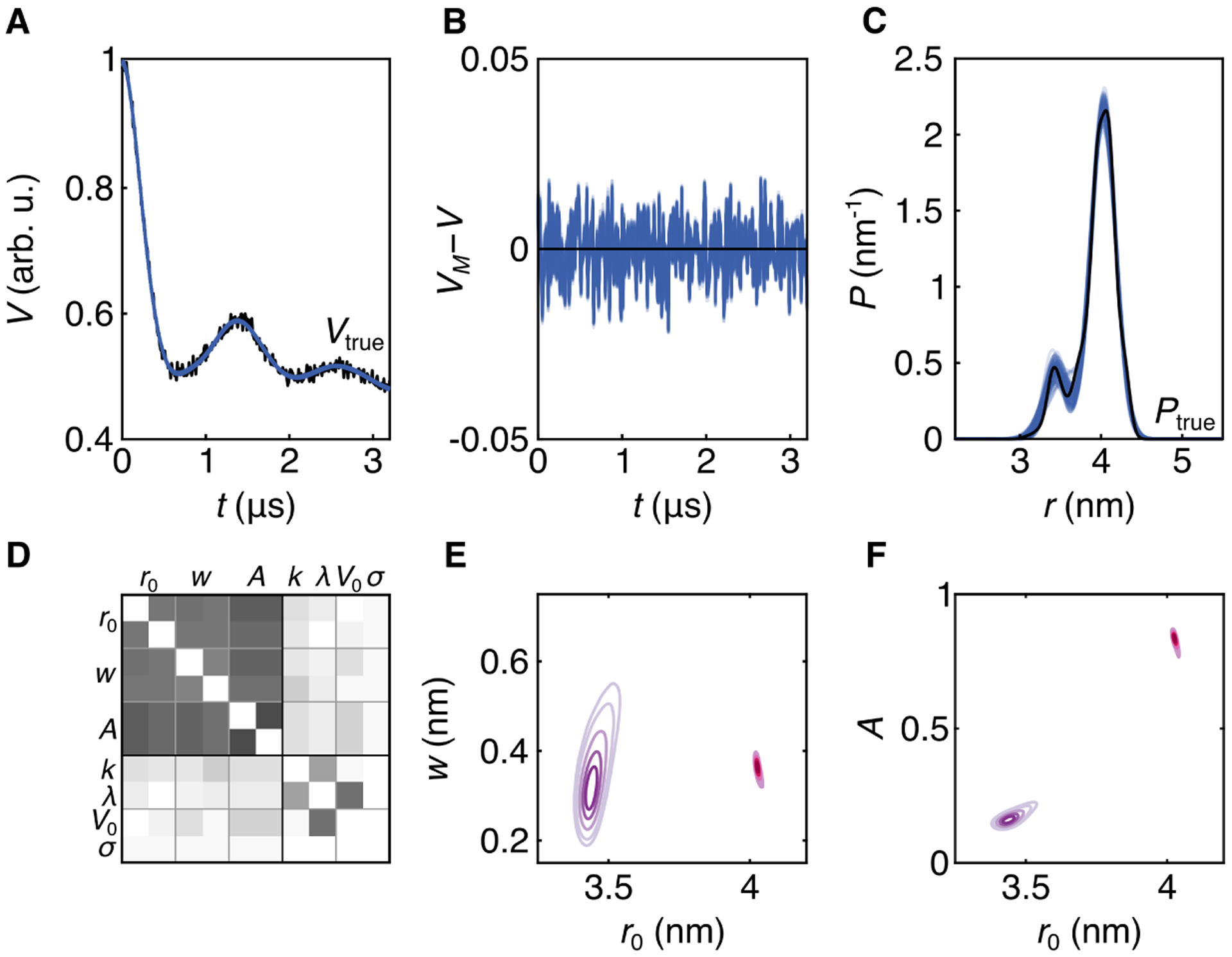
Bayesian inference with a two-Gaussian distribution model. A. Time-domain trace 36787 from synthetic data set (V_true(t)) (black) and 100 samples from the MCMC chains (blue). B. Residual analysis for the 100 MCMC samples (blue). C. Ensemble of 100 MCMC distributions (blue) and distance distribution 3223 from synthetic data set (black). D. Correlation matrix of all parameters, white indicating no correlation and black indicating full positive or negative correlation. E. 2D marginalized posteriors for widths and positions. The two Gaussian components are distinguished by color. F. 2D marginalized posteriors for amplitudes and positions, with identical coloring as E. The MCMC simulation was run with 5 chains with 30,000 posterior samples each.

Again, a valuable output of this method are the parameter correlations, visually summarized in panel D. All distribution parameters (r_0,i, w_i, A_i) are heavily correlated with one another while there is little correlation between distribution and time-domain parameters. The strongest correlation among time-domain parameters is between V₀ and λ. Panels E and F show the obtained 2D marginalized posteriors for the distance distribution parameters. As the position of the short-distance component increases, we see a corresponding increase in its width and in its amplitude. The posteriors for the longer-distance component are very tight, indicating high certainty. There is slight anticorrelation between position and both width and amplitude.

The next synthetic example, shown in Fig. 6, is a challenging, broad distribution with several poorly-resolved modes with similar intensities. The Bayesian analysis was conducted using a three-Gaussian distribution model. The ensemble of MCMC samples drawn from the posterior are shown in Fig. 6A, the ensemble of residuals in B, and the distribution ensemble in C. Although the model fits the data well (panels A and B), there is substantial scatter in the ensemble of distance distributions (panel C). This shows that the uncertainty about the shape is significant over the entire distribution. The long-distance edge at 4 nm is fairly well defined, but the location of the short-distance edge around 2 nm is less clear. The distribution ensemble shows that the data are not strong enough (i.e. too noisy or too short) to either exclude or confirm modes at 2.8 and 3.9 nm—although they reveal the possibility of such modes. Also, the location of the mode around 3.4 nm is uncertain. This shows again that it is important to consider a distribution ensemble instead of a single distribution in order to make robust conclusions.

Figure 6:

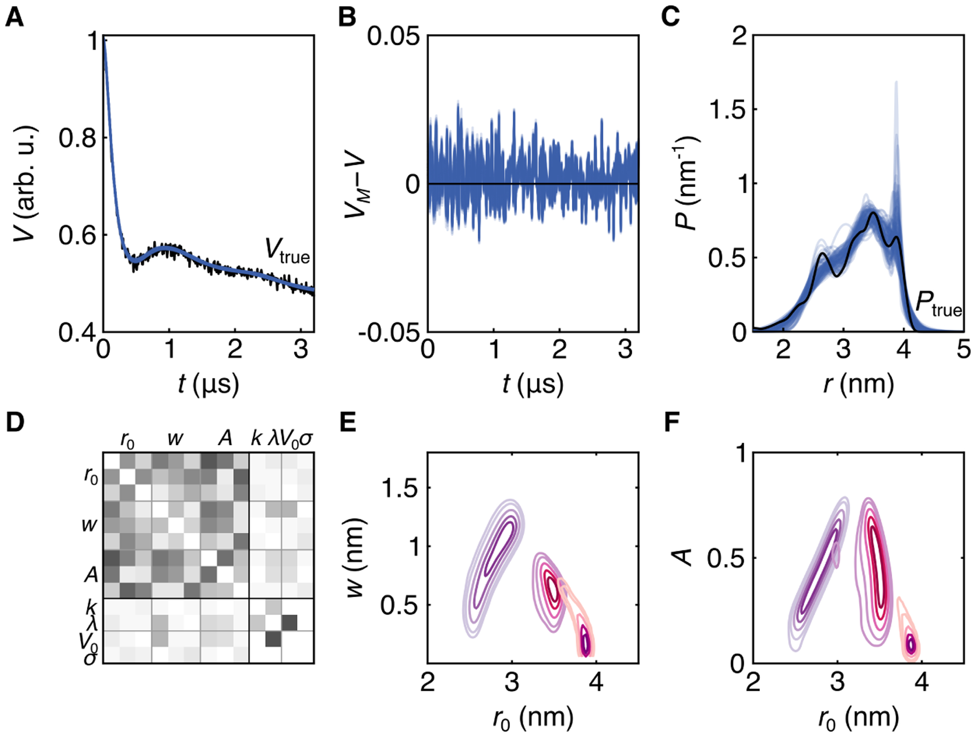
Bayesian inference with a three-Gaussian distribution model. A. Time-domain trace 51412 from synthetic data set (V_true(t)) (black) and 100 MCMC samples (blue). B. Residual analysis for all MCMC samples (blue). C. MCMC ensemble (blue) and distance distribution 4428 from synthetic data set (black). D. Correlation matrix of all parameters, white indicating no correlation and black indicating full positive or negative correlation. E. 2D marginalized posteriors for widths and positions. Individual components are distinguished by color. F. 2D marginalized posteriors for amplitudes and positions, with identical coloring as E. The MCMC simulation was run with 6 chains, with 40,000 posterior samples each.

The correlations between distribution parameters (Fig. 6D) vary but, as in the previous examples, the correlation between V₀ and λ is substantial. The 2D marginalized posteriors for the distribution parameters (Fig. 6E–F) show that there is significant uncertainty about the positions, widths, and amplitudes of the three Gaussian components. The reason for this uncertainty is that in the time-domain signal the noise level is significant relative to the shallow amplitude of the oscillations after the initial drop. The oscillations are shallow because of the large width of the underlying distribution.

6. Experimental example

So far, we have utilized synthetic data where we were able to pick ground-truth distributions that can be well approximated by a certain number of Gaussians. In this section, we demonstrate the method with experimental data, where this is not possible.

This brings up an important aspect of DEER data analysis, model checking and comparison.¹⁹ When the ground-truth distribution is not known, is is important to check whether a multi-Gauss model fits the data and to compare the quality of models with different numbers of Gaussians.

Figure 7A shows the DEER trace (black) that was collected to determine inter-subunit distances in SthK, a tetrameric bacterial cyclic nucleotide-gated (CNG) ion channel.³¹ Here we analyze the DEER trace using multi-Gauss models with 1 to 4 Gaussians (abbreviated as 1G, 2G, 3G, and 4G). Resulting ensembles of MCMC samples of signals, residuals, and distributions are shown in blue in Fig. 7A–C. Based on the systematic deviation of its residuals at early times, it is clear that the 1G model is inappropriate, even though it provides an apparently precise P(r) given how tight the distribution ensemble is. This is consistent with the fact that the ion channel is a homotetramer, and the distribution is expected to be at least bimodal. The 2G model matches the data better, but shows some systematic deviation in the residuals as well. The 3G and 4G models describe the signal similarly well, as their residuals are visually free of systematic deviations.

Figure 7:

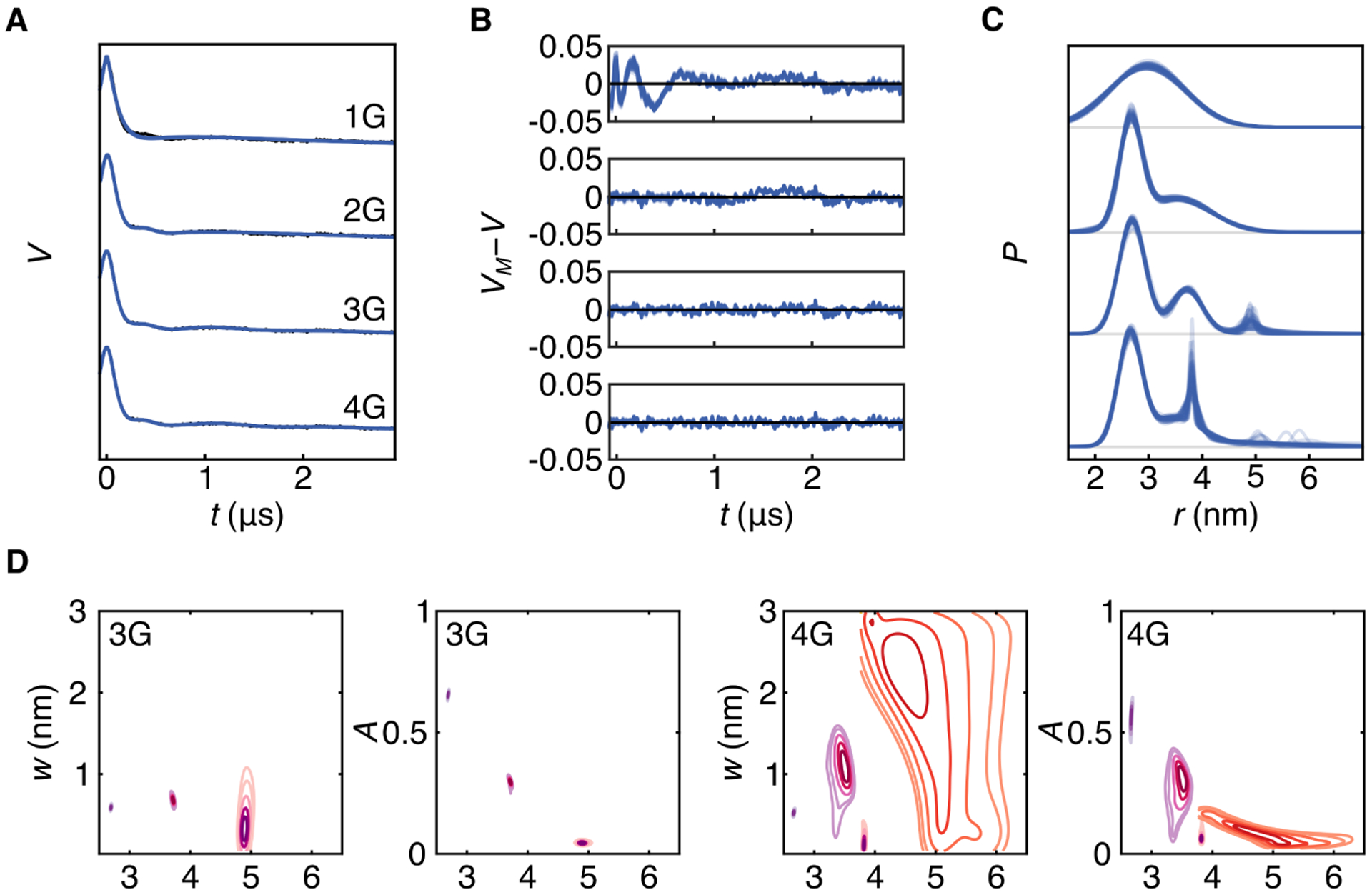
Bayesian inference using multi-Gauss models on a DEER trace obtained from the ion channel SthK D261R1.³¹ A. The raw experimental DEER data (black) and 50 MCMC ensembles from the analysis using 1-, 2-, 3-, and 4-Gaussian models (blue). B. Residuals based on the MCMC ensemble. C. Distance distribution ensembles for each of the four models. D. 2D marginalized posteriors for widths and positions for 3G and 4G models. Individual components are distinguished by color. Number of chains and posterior samples per chain for the MCMC simulations: 8 and 20,000 (1G), 5 and 30,000 (2G), 5 and 40,000 (3G), 5 and 80,000 (4G).

The distance distribution ensembles in Fig. 7C reveal some important details. In the 3G model, two components are quite certain, but the third at about 5 nm has large uncertainty in its width. In the 4G model, three of the components model the distribution below about 4 nm, and the fourth component is at long distances and is very uncertain both in width and position. This is also evident from the 2D marginalized posteriors shown in Fig. 7. Whereas all parameter posteriors are relatively tight for the 3G model, the posterior for the long-distance component of the 4G model is very delocalized in position and width. Overall, this suggests that the 4G model is likely overfitting the data.

Within the framework of Bayesian inference, a formal approach for model comparison is available. Two models M₁ and M₂ can be compared via the ratio p(M₁|V, I)/p(M₂|V, I) of their posterior probabilities.^19,32 This ratio is called the posterior odds and is calculated via

$$\underset{\text{posterior odds }}{\underbrace{\frac{p\left(M_2\mid V,I\right)}{p\left(M_1\mid V,I\right)}}}=\underset{\text{Bayes factor }{B}_{2,1}}{\underbrace{\frac{p\left(V\mid M_2,I\right)}{p\left(V\mid M_1,I\right)}}}\cdot \underset{\text{prior odds }}{\underbrace{\frac{p\left(M_2\mid I\right)}{p\left(M_1\mid I\right)}}}$$ (22)

where the first ratio on the right-hand side is known as the Bayes factor, and the second ratio is called the prior odds. The posterior odds summarize how much one model is favored over the other in light of the data and prior information. The Bayes factor represents how likely the data are assuming one model vs. assuming the other. The prior odds quantify the odds for or against one model, prior to taking into account the data. In most applications, this ratio is set to one (encoding no preference).¹⁹ Then the Bayes factor equals the posterior odds and can be used to quantify how the data speak for one model over the other. As a rule of thumb, log₁₀ B_2,1 > 8 can be seen as relatively strong indication for M₂ over M₁.³³ In a comparison of two models that belong to the same family of models, or when one model is a superset of the other (e.g. the 3G model is a superset of the 2G model), the Bayes factor penalises complicated models that might be prone to overfitting.¹⁹ In such cases, if the data are better explained by the simpler model, the Bayes factor in favor of the more complex model is typically small.

The Bayes factors B_m,1 for all m-Gauss models relative to the 1G model are shown in Fig. 8. They show that the 2G model is clearly preferable over 1G, and give preference for 3G and 4G over 2G (log₁₀B_3,2 ≈ 25 and log₁₀B_4,2 ≈ 30). However, there is only a small difference between 3G and 4G, and the Bayes factor log₁₀B_4,3 ≈ 5 indicates that the 4G model does not describe the data much better than the 3G model. In combination with the delocalized posterior, this is a strong indication that the 4G model is overfitting the data.

Figure 8:

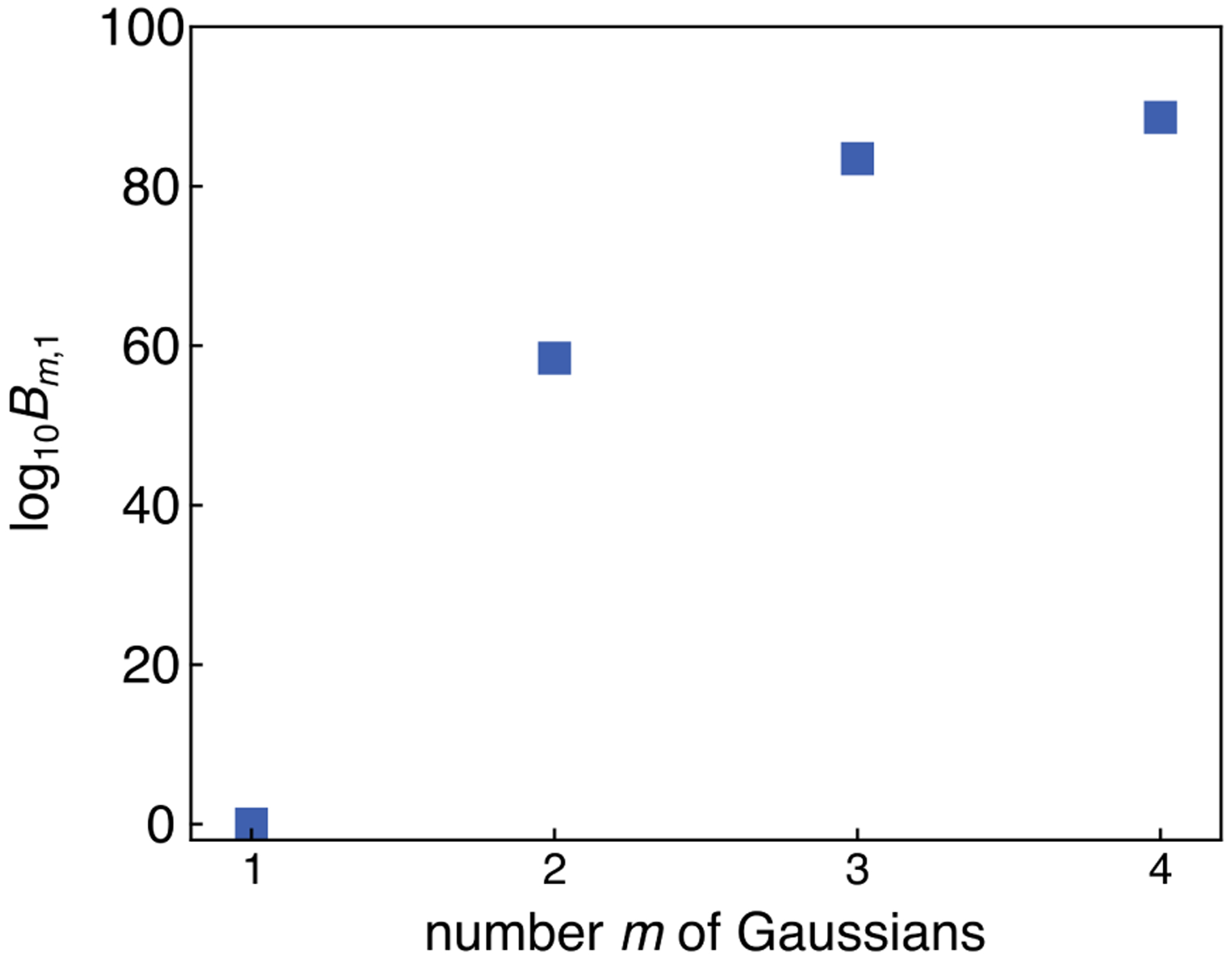
Bayes factors comparing the four models from Fig. 7 to the 1G model.

Neither residuals nor Bayes factors alone are enough for a complete analysis. While the latter compare two models and help with identifying overfitting, they do not contain information on whether the chosen models is appropriate and gives a good fit to the data. Instead, an inadequate model with systematic misfitting can be diagnosed through the residuals. Additionally, even if a model fits the data well and has the largest Bayes factor among a set of models, it might still be physically inappropriate, and considerations outside the Bayesian analysis framework must be used to determine a more appropriate model.

The model comparison outlined here allows assessment of an appropriate number m of Gaussians. This is analogous to selecting an appropriate α regularization parameter in Tikhonov regularization.¹⁴ However, although these selection methods are quantitative, they are not unique and therefore fully objective.

7. Conclusions

The Bayesian inference approach presented here fully quantifies the uncertainty in model parameters obtained from fitting DEER data using a parametric multi-Gauss distribution model. Its advantage over a least-squares fitting approach is that it provides the posterior distribution that completely quantifies model parameter uncertainty, whereas least-squares fitting only determines a point estimate with confidence intervals. The posterior allows the analysis of spread and asymmetry in the parameter distributions, and of correlations between model parameters.

We showed that a small ensemble of distributions drawn from the MCMC samples is well suited to visually capture both uncertainty and correlation in distance distribution plots. Therefore, it should be preferred over error bands. We also illustrated how to use a combination of residuals, parameter posteriors, and Bayes factors to help with model comparison and to identify under- and overfitting. This can be expanded to include other modern Bayesian methods for model comparison as well.¹⁹

Although we have presented the probabilistic approach using an exponential model for V_inter(t) and a multi-Gauss model for P(r), the approach is very general. It is applicable to any other parametric models of V_inter(t) and P(r). The background can be extended to include fractal dimensions³⁴ and to allow for excluded-volume effects.³⁵ The distance distribution basis functions are not limited to Gaussians; other functions such as 3D Rice functions can be used,³⁶ particularly in cases where there is no clear fit to a sum of Gaussians via residual and Bayes factor analysis. If the noise level is known experimentally (e.g. from analyzing the variance among a series of sequentially acquired traces), then it can be fixed and omitted as a model parameter. In the case the noise level is not constant across the trace, a more sophisticated noise model can be included.

In principle, the probabilistic inference methodology used here for multi-Gauss models is equally applicable to the non-parametric models for P(r) used in Tikhonov regularization. However, this requires substantially more sophisticated considerations about the prior for P(r) and the MCMC sampling procedure, and is therefore left for future research. Once this is accomplished, a meaningful quantitative and systematic comparison between multi-Gauss and Tikhonov models within a Bayesian framework will be possible.

References

- (1).Milov AD; Salikhov KM; Shchirov MD Application of the Double Resonance Method to Electron Spin Echo in a Study of the Spatial Distribution of Paramagnetic Centers in Solids. Sov. Phys. Solid State 1981, 23, 565–569. [Google Scholar]
- (2).Milov AD; Tsvetkov YD Double Electron–Electron Resonance in Electron Spin Echo: Conformations of Spin-Labeled Poly-4-Vinylpyridine in Glassy Solutions. Appl. Magn. Reson 1997, 12, 495–504. [Google Scholar]
- (3).Pannier M; Veit S; Godt A; Jeschke G; Spiess HW Dead-Time Free Measurement of Dipole–Dipole Interactions between Electron Spins. J. Magn. Reson 2000, 142, 331–340. [DOI] [PubMed] [Google Scholar]
- (4).Jeschke G; Polyhach Y Distance Measurements on Spin-Labelled Biomacromolecules by Pulsed Electron Paramagnetic Resonance. Phys. Chem. Chem. Phys 2007, 9, 1895–1910. [DOI] [PubMed] [Google Scholar]
- (5).Jeschke G DEER Distance Measurements on Proteins. Annu. Rev. Phys. Chem 2012, 63, 419–446. [DOI] [PubMed] [Google Scholar]
- (6).Matveeva AG; Nekrasov VM; Maryasov AG Analytical Solution of the PELDOR Inverse Problem Using the Integral Mellin Transform. Phys. Chem. Chem. Phys 2018, 19, 32381–32388. [DOI] [PubMed] [Google Scholar]
- (7).Worswick SG; Spencer JA; Jeschke G; Kuprov I Deep Neural Network Processing of DEER Data. Sci. Adv 2018, 4, eaat5218. [DOI] [PMC free article] [PubMed] [Google Scholar]
- (8).Jeschke G; Koch A; Jonas U; Godt A Direct Conversion of EPR Dipolar Time Evolution Data to Distance Distributions. J. Magn. Reson 2002, 155, 75–82. [DOI] [PubMed] [Google Scholar]
- (9).Chiang Y-W; Borbat PP; Freed JH Maximum Entropy: A Complement to Tikhonov Regularization for Determination of Pair Distance Distributions by Pulsed ESR. J. Magn. Reson 2005, 177, 184–196. [DOI] [PubMed] [Google Scholar]
- (10).Jeschke G; Chechik V; Ionita P; Godt A; Zimmermann H; Banham J; Timmel CR; Hilger D; Jung H Deer-Analysis2006—A Comprehensive Software Package for Analyzing Pulsed ELDOR Data. Appl. Magn. Reson 2006, 30, 473–498. [Google Scholar]
- (11).Sen KI; Logan TM; Fajer PG Protein Dynamics and Monomer-Monomer Interactions in AntR Activation by Electron Paramagnetic Resonance and Double Electron-Electron Resonance. Biochem. 2009, 46, 11639–11649. [DOI] [PubMed] [Google Scholar]
- (12).Brandon S; Beth AH; Hustedt EJ The Global Analysis of DEER Data. J. Magn. Reson 2012, 218, 93–104. [DOI] [PMC free article] [PubMed] [Google Scholar]
- (13).Stein RA; Beth AH; Hustedt EJ A Straightforward Approach to the Analysis of Double Electron–Electron Resonance Data. Methods Enzymol. 2015, 563, 531–567. [DOI] [PMC free article] [PubMed] [Google Scholar]
- (14).Edwards TH; Stoll S Optimal Tikhonov Regularization for DEER Spectroscopy. J. Magn. Reson 2018, 288, 58–68. [DOI] [PMC free article] [PubMed] [Google Scholar]
- (15).Fábregas Ibáñez L; Jeschke G; Stoll S DeerLab: A Comprehensive Toolbox for Analyzing Dipolar EPR Spectroscopy Data. Magn. Reson 2020, in review. [DOI] [PMC free article] [PubMed] [Google Scholar]
- (16).Edwards TH; Stoll S A Bayesian Approach to Quantifying Uncertainty from Experimental Noise in DEER Spectroscopy. J. Magn. Reson 2016, 270, 87–97. [DOI] [PMC free article] [PubMed] [Google Scholar]
- (17).Hustedt EJ; Marinelli F; Stein RA; Faraldo-Gómez JD; Mchaourab HS Confidence Analysis of DEER Data and its Structural Interpretation with Ensemble-Biased Metadynamics. Biophys. J 2018, 115, 1200–1216. [DOI] [PMC free article] [PubMed] [Google Scholar]
- (18).Jaynes ET Probability Theory. The Logic of Science; Cambridge University Press: St. Louis, 2003. [Google Scholar]
- (19).Gelman A; Carlin JB; Stern HS; Dunson DB; Vehtari A; Rubin DB Bayesian Data Analysis; CRC Press: Boca Raton, 2014. [Google Scholar]
- (20).Murphy KP Machine Learning: A Probabilistic Perspective; MIT Press: Cambridge, 2012. [Google Scholar]
- (21).McElreath R Statistical Rethinking. A Bayesian Course With Examples in R and STAN; CRC Press: London, 2020. [Google Scholar]
- (22).Hoffman MD; Gelman A The No-U-Turn Sampler: Adaptively Setting Path Lengths in Hamiltonian Monte Carlo. J. Mach. Learn. Res 2014, 15, 1593–1623. [Google Scholar]
- (23).Betancourt M A Conceptual Introduction to Hamiltonian Monte Carlo. arXiv eprints 2017, arXiv:1701.02434 [stat.ME]. [Google Scholar]
- (24).Salvatier J; Wiecki TV; Fonnesbeck C Probabilistic Programming in Python Using PyMC3. PeerJ Comput. Sci 2016, 2, e55. [DOI] [PMC free article] [PubMed] [Google Scholar]
- (25).Gelman A; Rubin DB Inference from Iterative Simulation Using Multiple Sequences. Stat. Sci 1992, 7, 457–472. [Google Scholar]
- (26).Brooks SP; Gelman A General Methods for Monitoring Convergence of Iterative Simulations. J. Comput. Graph. Stat 1998, 7, 434–455. [Google Scholar]
- (27).Vehtari A; Gelman A; Simpson D; Carpenter B; Bürkner P-C Rank-Normalization, Folding, and Localization: An Improved for Assessing Convergence of MCMC. arXiv e-prints 2019, arXiv:1903.08008 [stat.CO]. [Google Scholar]
- (28).Stephens M Dealing with Label Switching in Mixture Models. J. R. Stat. Soc. B 2000, 62, 795–809. [Google Scholar]
- (29).Jasra A; Holmes CC; Stephens DA Markov Chain Monte Carlo Methods and the Label Switching Problem in Bayesian Mixture Modeling. Stat. Sci 2005, 20, 50–67. [Google Scholar]
- (30).Edwards TH; Stoll S Synthetic Test Data Set for DEER Spectroscopy Based on T4 Lysozyme. DOI: 10.6069/H5S75DCG, 2018. [DOI] [Google Scholar]
- (31).Evans EGB; Morgan JLW; DiMaio F; Zagotta WN; Stoll S Allosteric Conformational Change of a Cyclic Nucleotide-Gated Ion Channel Revealed by DEER Spectroscopy. Proc. Nat. Acad. Sci. USA 2020, 117, 10839–10847. [DOI] [PMC free article] [PubMed] [Google Scholar]
- (32).Kass R; Raftery E Bayes Factors. J. Am. Stat. Assoc 1995, 90, 773–795. [Google Scholar]
- (33).Thrane E; Talbot C An Introduction to Bayesian Inference in Gravitational-Wave Astronomy: Parameter Estimation, Model Selection, and Hierarchical Models. Publ. Astron. Soc. Aust 2019, 36, e010. [Google Scholar]
- (34).Kutsovsky YE; Mariasov AG; Aristov YI; Parmon VN Electron Spin Echo as a Tool for Investigation of Surface Structure of Finely Dispersed Fractal Solids. React. Kinet. Catal. Lett 1990, 42, 19–24. [Google Scholar]
- (35).Kattnig DR; Reichenwallner J; Hinderberger D Modeling Excluded Volume Effects for the Faithful Description of the Background Signal in Double Electron–Electron Resonance. J. Phys. Chem. B 2013, 117, 16542–16557. [DOI] [PubMed] [Google Scholar]
- (36).Domingo Köhler S; Spitzbarth M; Diederichs K; Exner TE; Drescher M A Short Note on the Analysis of Distance Measurements by Electron Paramagnetic Resonance. J. Magn. Reson 2011, 208, 167–170. [DOI] [PubMed] [Google Scholar]