Abstract
This paper studies the dynamics of human mobility during the initial stage of the COVID-19 pandemic in countries around the world. The main goal of the analysis is to empirically separate voluntary reductions in mobility driven by the information about the location-specific pandemic trends from the effects of the government-imposed social distancing mandates. Google human mobility dataset is used to track the dynamics of mobility across a wide range of categories (e.g., workplace, retail and recreational activities, etc.), while information on country-specific counts of COVID-19 cases and deaths is used as a proxy for the information about the spread of the pandemic available to the population. A detailed index of stringency of the government-imposed social distancing policies in around 100 countries is used as a measure of government response. We find that human mobility does respond in a significant way to the information about the spread of the pandemic. This channel can explain about 15 percentage points of the overall reduction in mobility across the affected countries. At the same time, our results imply that government-imposed policies account for the majority of the reduction in the mobility observed during this period.
Keywords: COVID-19, Mobility, Government response, Information, Group fixed effects
1. Introduction
The rapid spread of COVID-19 pandemic in early 2020 has produced a variety of policy responses in countries around the world designed to limit the proliferation of the virus and alleviate the pressure on the health systems. These measures ranged from very drastic lockdown policies implemented in parts of Asia and Southern Europe to less stringent approaches implemented elsewhere (e.g. Sweden). As of mid-2020, the policy landscape continues to evolve rapidly with a wide array of measures continuing to be implemented and relaxed in different jurisdictions in response to the changing pandemic situation. At the same time, the benefits and cost of the various policy options continue to be the topic of debate in press and policy discussions.
Existing empirical evidence demonstrates a clear impact of the reduction in human mobility on the virus growth rates (Soucy et al., 2020; Fang et al., 2020; Prem et al., 2020). There is also a growing literature studying how different social distancing policies affect mobility, most of which is based on the US data (see for example Engle et al., 2020; Brzezinski et al., 2020; Maloney and Taskin, 2020). This type of evidence is particularly important from the economic point of view because measures aimed at reducing mobility, such as public information campaigns, closures of schools and retail outlets, personal movement restrictions, shelter-in-place orders and lockdowns differ significantly in their economic and labour market effects.
The problem of evaluating these policies is further complicated by the presence of individual behavioural adjustments (also called community responses) that are independent of the government policies. A large body of evidence in economics demonstrates that people tend to respond rationally to the information and adjust their choices and behaviours in the presence of health and other types of risk. In the case of the COVID-19 pandemic, relatively little was known about the health risk posited by the virus at the time the first lockdown policy was introduced in Wuhan, China in January 2020. However, when comparable measures were later rolled out in other parts of the world, they were implemented against the background of the damage caused by the COVID-19 pandemic in Northern Italy, Spain, NYC and other virus hotspots. It is likely that the new information about the spread and damage of COVID-19 abroad and domestically has led to significant behavioural adjustments, before and independently of the social distancing measures mandated by the governments.
The objective of this study is to empirically evaluate the impact of the stringency of government responses to the pandemic on human mobility in affected countries and to separate it from the impact of self-imposed behavioural adjustments arising in the affected populations. To do this we combine Google human mobility data with information on the type, timing and stringency level of the social distancing policies implemented in a given country over the course of the initial stage of pandemic. The data on country-specific counts of COVID-19 cases and deaths are used as a proxy for the information available to the population about the stage of the pandemic in each location. The temporal proximity of the news about the spread of the pandemic in a given country and the implementation of social distancing policies makes it challenging to separate the effect of policies from the individual behavioural adjustments empirically. We use precise and flexible modelling of the effects of social distancing policies to estimate the relationship between mobility and COVID-19 cases and mortality conditional on the timing of these policies as well as other determinants of human mobility such as daily ambient temperature, days of the week and time trends. The identification of the community response effect relies on the differences in the time paths of the cumulative COVID-19 cases and deaths between countries that are similar in terms of all other characteristics included in the models.
We estimate a series of models with country fixed effects, cumulative cases, time trends and interactions between policies, regions and stages of the pandemic, to explore cross-country heterogeneity in the effects of the COVID-19 policies and information on human mobility. Our results show the presence of significant community response to the information about the spread of the pandemic in the form of reduced mobility that is independent of government social distancing measures and often precedes them. This decline is mostly driven by the country's cumulative case count, while the number of COVID-19 related deaths has a relatively small effect. At the same time, our results imply that the magnitude of the community response is relatively small and can account for at most 15 percentage points of the post-pandemic decline in most types of economically relevant mobility. The effect of government-implemented policies turns out to be much larger. Cumulatively they can account for up to 50 percentage points of permanent reductions in mobility across countries in our sample. More stringent policies, such as restrictions on international travel, school and workplaces closing, and restrictions on internal movements each have large negative and statistically significant effects on mobility of about 5–15 percentage points.
Overall, these results based on high-frequency mobility data across a large sample of countries imply that, if policymakers adopt the strategy of reducing the amount of physical contact amongst people to stop the spread of the pandemic, government-mandated social distancing measures are necessary. Relying on community response alone is unlikely to achieve this goal for the majority of countries. At the same time, presence of significant community response driven by the information about the spread of the virus implies that relaxation of the social distancing policies is unlikely to lead to rapid economic recovery in most of the affected countries and the perceived health risks will continue to impact consumer confidence for a substantial portion of the population.
The rest of the paper is organised as follows. Section 2 reviews economic and epidemiological studies on the behavioural responses to health risk and the emerging economics literature on the policy response to the COVID-19 pandemic relevant for this study. Section 3 describes the data used in the analysis and discusses the patterns across different mobility types that were present at the start of the pandemic in various countries and regions of the world. It also summarises the evidence on the evolution of policy response across countries. Section 4 discusses the empirical models and Section 5 presents the main results. Section 6 concludes with a brief discussion and suggestions for future research. Additional empirical results and robustness checks are presented in the Appendix to the paper.
2. Related literature
The study of mobility patterns is an essential component in understanding the spread of epidemics. Human-to-human contact is one of the major transmission mechanisms for many viral outbreaks and changes to social interactions have been studied in the context of many recent viral infections (Rasul, 2020). Changes in human mobility and related policy measures have been used to explain the diffusion of previous pandemics, such as the 1918 Influenza Pandemic, Ebola, and the 2009 H1N1, (see for example Hatchett et al., 2007; ), and to understand how travelling flows and changes in human behaviours may alter the epidemic spreading (Meloni et al., 2011). An important component of these analyses is to understand whether changes in behaviours are mostly triggered by policy decisions or rather by the transmission of information from other sources, such as media and local interpersonal contacts. Recent studies have shown that human mobility and social activity are affected by social connections (Charoenwong et al., 2020) and by risks of infection and therefore optimal policies should keep these factors into consideration (Farboodi et al., 2020). Previous literature showed that how self-initiated changes in behaviours are very hard to model and fully understand, because of lack of suitable data (Meloni et al., 2011; Tizzoni et al., 2014).
The number of existing studies in scientific disciplines using mobility data around epidemics is relatively limited, and most of these analyses use small datasets, which only address selected aspects of mobility. For example, Meloni et al. (2011) use simulation based on airport network data to show that self-driven changes in mobility may worsen the spread of disease, as individuals move to avoid areas with a high prevalence of infections. Similarly, Tizzoni et al. (2014) use metapopulation models to show that commuting networks from mobile phone data capture the vast majority of total mobility fluxes and therefore can effectively be used in epidemic models for influenza-like-illnesses. In general, as discussed in Zhu et al. (2017), individual behaviours and compliance to policy recommendations during a health crisis are an important determinant of the overall impact of the epidemic on the society. Existing literature in the field has shown that so-called “non-pharmaceutical interventions”, such as school closures and other policies aimed at reducing mobility and social interaction have been effective in limiting the spread of previous pandemics (see for example Hatchett et al., 2007; Litvinova et al., 2019, amongst many others).
Economists have started to engage with this debate in recent years. Adda (2016) analyses the effect of policies limiting interpersonal contacts (such as school and public transport closures and expansion of railways networks) on the spread of three major viral diseases (influenza, gastroenteritis and chickenpox) and shows that these policies have major effects in reducing the disease spread but are not always cost-effective. Further, school closures have a noticeable effect on reducing diseases’ spread for children but may increase the spread of the disease for the elderly in the short-run. Orset (2018) analyses the attitude of French people to home confinement during an influenza pandemic and shows that over three-quarters of respondents indicate compliance with this measure, even if individuals’ reactions vary with socio-economic characteristics and direct experience with the infection.
Changes in activity levels around epidemics have been studied by economists and epidemiologists. The so-called “prevalence response” refers to individuals’ attempts to protect themselves and limit the spread of infections (see for example Lakdawalla et al., 2006, amongst others). The 2003 SARS epidemic dramatically decreased people's activity in restaurants, shopping centres and public places (Chou et al., 2004; Siu and Wong, 2004) and it also led to a decrease in people's demand for health care and outpatients’ visits (Hsieh et al., 2004). Bennet et al. (2015) compare individuals’ responses to public and private signal during 2003 SARS epidemic in Taiwan and show that the response to the public (SARS official reports) and private (peers’ behaviour) information have similar elasticities.
Behavioural responses after health crises or natural disasters, and the role of new information around disease outbreaks, have also been analysed by economists. Existing studies have analysed several changes in behaviours, including the adoption of very simple low-cost changes in daily habits, like hand-washing (Agüero and Beleche, 2017), and changes in risk-taking behaviours, related to health (de Paula et al., 2014) or general life (Page et al., 2014). Further, individuals may change their behaviours and beliefs in response to the increased risk and uncertainty from viral outbreaks and governments’ public health alerts (Rasul, 2020; Junior and Rasul, 2018). This may include changes in social interactions, which may have important economic and social consequences (Fogli and Vedkamp, 2019).
Recent evidence on the COVID-19 pandemic in the United States has shown that lockdown policies have significantly reduced mobility (Engle et al., 2020; Malonei and Taskin, 2020; Painter and Qu, 2020) and that this effect is mediated by States’ characteristics, such as political preferences, education levels and socioeconomic status (Brzezinski et al., 2020). Cronin and Evans (2020) compare the impact of state-level policies to that of self-regulating behaviour on mobility across the US states using the cell-phone data and find that private self-imposed reductions in mobility played an important role in reducing the foot traffic to restaurants, hotels, and entertainment venues. They estimate that self-imposed behaviours account for a large fraction (up to 80%) of decline in discretionary mobility. Our estimates of the self-regulating community response in the sample of 87 countries across all regions of the world are much smaller than those reported in the US literature to date (in particular Cronin and Evans, 2020), with the majority of the response driven by the government mandates.
Previous economic studies have used Google trend data in the context of health and labour market (see for example Dukic et al., 2012; Kearney and Levine, 2015; Aguero and Beleche, 2017; Gonzalez-Fernandez and Gonzalez-Velasco, 2018), but the new Google mobility dataset allows a completely different level of analysis of mobility. Further, we analyse several determinants of mobility, including the country's characteristics, and new information about the pandemic, and show how individuals in different countries adjust their mobility patterns, based on these different factors.
3. Data and descriptive statistics
3.1. Data sources
The data on human mobility by country are drawn from the Community Mobility Reports released by Google for 133 countries. These reports are created with aggregated, anonymized sets of data from users’ mobile device Location History and are segmented into six location categories: retail and recreation, grocery and pharmacy, parks, public transportation, workplaces and residential areas. The reports show how visits to and length of stay at different categories of locations change over time compared to a baseline on the 15th February 2020. These human mobility measures are tracked by Google daily and in a consistent manner across the countries. The data release that is used in this paper covers the period from February 15th 2020 to May 15th 2020 inclusive, however, we are only using mobility data up to April 20th 2020, as this was the period covered by the OxCGRT dataset (described below) at the time of writing.
COVID-19 policy responses are derived from the Oxford COVID-19 Government Response Tracker (OxCGRT) database (Thomas et al., 2020), which provides daily information for 150 countries on government responses to COVID-19 epidemic, including policies restricting human mobility, financial and economic stimulus packages, public health interventions, etc. The sets of policies included in the OxCGRT and their stringency gradations change between different releases of the database. In the main analysis, we use the second release of these data that covers the period from January 1st 2020 to April 20th 2020. This dataset includes seven policies aimed at restricting human mobility to slow down the spread of the COVID-19 epidemic. The policies and their stringency levels are as follows: (1) public information campaigns (no measure or implemented); (2) international travel controls (no measure, screening, quarantined arrivals from high-risk regions, ban on arrivals from high-risk regions); (3) cancellation of public events; (4) closing of public transportation; (5) closing of schools; (6) closing of workplaces; and (7) restrictions on internal movements (stringency levels for policies 4–7 are no measure, recommended closing or restriction, required closing or restriction).
It must be noted that starting from April 6th 2020 information about the COVID-19 measures is increasingly incomplete in the April 20th release. To rectify this issue the dates between April 6th and April 20th use COVID-19 policy information merged from the later, April 29th 2020, OxCGRT release. The OxCGRT April 29th 2020 release specifies a more fine-grained classification of stringency levels for some policies and includes two additional policies such as restrictions on gatherings (with five stringency levels depending on the size of the groups not allowed to gather), and stay at home policy (with four stringency levels). Unfortunately, a large number of countries do not have a complete record of these additional policies. For this reason, we focus the main empirical analysis on the seven policies discussed above and analyse the extended set of nine policies with the updated stringency levels using a smaller sample of countries in the Robustness section.
We use daily counts of COVID-19 cases and deaths at the national level available from a variety of sources (e.g. European Centre of Disease Prevention and Control COVID-19 cases and deaths database) as a measure of information about the pandemic spread available to the population at a given point in time. The data release that we use covers the period from January 1st until April 20th and the data is available for 202 countries. In total 109 countries have data on the three groups of variables (Google mobility, COVID-19 cases and deaths and COVID-19 government response measures) for the period February15th-April 20th 2020. We supplement these country-level time series data with daily temperature records to use as a control in the cross-country regressions. We were able to obtain daily temperature records for the period from January 1st to April 20th of 2020, for 94 countries in our sample.
3.2. Sample construction
The goal of this paper is to estimate how the changes in information about the spread of the COVID-19 epidemic affected community mobility, conditional on any government policies implemented at that time. To answer this question we must consider countries at the very early stages of the epidemic. This will allow us to track the community responses to the first COVID-19 cases which are plausibly exogenous to community mobility as for the majority of countries most of these cases have originated from travelling abroad and are limited to travellers themselves and their families and acquaintances. These considerations necessitate restricting the analysis to countries that have experienced the first COVID-19 case after the starting date of the Google mobility data, namely 15/2/2020. To minimize concerns about the endogeneity of cases with respect to mobility it is also important to limit the sample to a relatively short period after the start of the pandemic. The data also need to include some pre-pandemic time periods as a benchmark against which mobility after the onset of the epidemic will be compared. As a compromise between a sufficiently long pre-pandemic period and a sufficiently large number of countries in the estimation sample, we set the pre-pandemic period equal to 5 days.
Further, our main sample only includes data for the first 21 days after the first COVID-19 case. This period is long enough for most countries to go from pre-epidemic mobility steady-state to the new lower mobility steady-state due to COVID-19 epidemic and for implementing a whole range of restrictive policies. Overall, our main estimation sample includes 73 countries in 6 world regions, which are observed for the 5 days before the first COVID-19 case and 21 days after. The list of these countries is given in the Appendix in Figures A1-A6. We denote the day when the first COVID-19 case was recorded as Period 0.
We impose these sample restrictions because we are interested in estimating the effect of the COVID-19 cases at the very beginning of the COVID-19 epidemic. Therefore, it is essential to observe the countries before and during the first weeks after the onset of the epidemic, which limits us to countries where the epidemic started after February 15th 2020 (the start of the Google mobility data).1 In principle, if we had data on absolute human mobility (e.g. the number of trips to different localities, etc.) we could have included the countries where the epidemic started before 15/02/2020 to help identify the effects of the COVID-19 cases beyond the first few cases, under the assumption that the pre-epidemic trend in mobility in these countries is similar to that of the countries observed before the onset of the epidemic. However, Google data measure the percentage change in mobility relative to February 15th, not the absolute levels of mobility. Since these countries are likely to have experienced epidemic-related declines in the absolute levels of mobility by February 15th, a given absolute change in mobility will amount to larger percentage change relative to February 15th than relative to a pre-epidemic period for these countries. Therefore using these countries in the estimation sample may cause an upward bias (in absolute terms) in the estimated effects if the interest lies in estimating the effects of policies and COVID-19 cases and mortality on percentage changes in mobility relative to pre-epidemic period.
Overall, using a longer sample period with a larger number of countries would not allow us to derive more reliable estimates of the effects of COVID-19 cases and policies on mobility and would also increase the risk of capturing spurious effects, such as a reduction in cases due to restrictions to mobility (rather than vice versa). Nevertheless, we relax one of these restrictions by including countries where the epidemic started before 15/02/2020, but still limiting the observation window to 21 days after the start of the epidemic. This extended sample includes 90 countries in 7 world regions. Results from this extended sample are very similar to those based on the main sample. They are discussed in Section 5.2 and are available in the Appendix.
3.3. Descriptive statistics
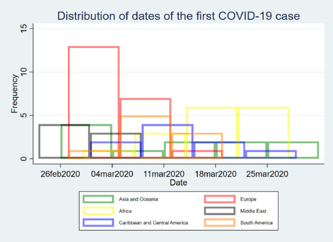
In the descriptive graphical analysis of the key variables and the regression analysis we focus on the time period of 5 days before the onset of the epidemic (i.e. first recorded COVID-19 case) and 21 days after the onset, provided that this period is within the data availability window of February 15th-April 20th 2020. This study period will occur at different calendar dates for different countries. For the vast majority of countries, this study period includes the implementation of most of the seven COVID-19 measures included in the OxCGRT database. Fig. 1 shows the distribution of the calendar date of the onset of COVID −19 epidemic (i.e. the date when the first COVID-19 case was recorded) for 73 countries in our sample. The date of the start of the epidemic ranges between 23rd of February 2020 and 27th of March 2020. Countries of the Middle East and Europe cluster in the first half of this period, whereas African countries tend to record their first COVID-19 case in the second half of the period. Countries from other regions have COVID-19 starting dates that are more uniformly spread over the period.
Fig. 1.
Distribution of the dates of the start of CODIV-19 epidemic.
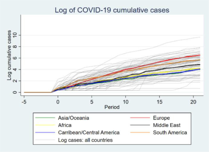
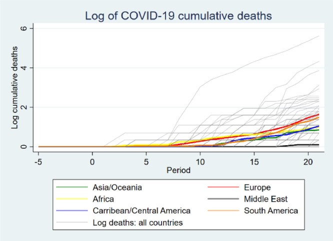
Fig. 2, Fig. 3 represent the (log) number of cases and deaths in the various regions included in the estimation sample. These graphs show the speed of the evolution of the pandemic in the different geographical areas considered in the analysis. Europe and South America show the highest number of cases and deaths in the period considered. By the 21st day from the start of the epidemic, the cumulative number of COVID-19 cases in our sample varied between 2 (in Papua New Guinea) and 15,679 (Turkey). The median number of cases was 219, and the 10% of countries with the largest number of cases are as follows: Austria (1332 cases), Czechia (1165 cases), Denmark (1115 cases), Netherlands (2460 cases), Norway (1423 cases), Portugal (2060 cases), Switzerland (2650 cases), Turkey (15,679 cases). As for the COVID-19-related deaths, by the 21st day of the epidemic, the median number was 3, with 10% of countries recoding 12 or more deaths.
Fig. 2.
Logarithm of COVID-19 cases. Note: On this figure zero on the vertical axis corresponds to zero recorded COVID-19 cases, while 0.35 corresponds to one recorded COVID-19 case. For COVID-19 casesthat are equal or greater than two the vertical axis measures their natural logarithm. Thin grey lines depict the trajectory of cases for each country in the sample. Thick coloured lines depict the average number of cases among countries within each region for each of the days of the COVID-19 epidemic included in the sample.
Fig. 3.
Logarithm of COVID-19 related deaths in the estimation sample. Note: On this figure zero on the vertical axis corresponds to zero recorded COVID-19 deaths, while 0.35 corresponds to one recorded COVID-19 death. For COVID-19 deaths that are equal or greater than two the vertical axis measures their natural logarithm. Thin grey lines depict the trajectory of deaths for each country in the sample. Thick coloured lines depict the average number of deaths amongst countries within each region for each of the days of the COVID-19 epidemic included in the sample. (For interpretation of the references to colour in this figure legend, the reader is referred to the web version of this article.)
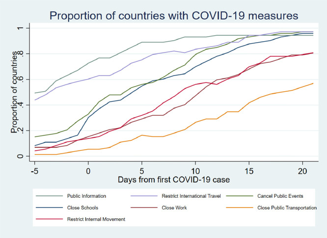
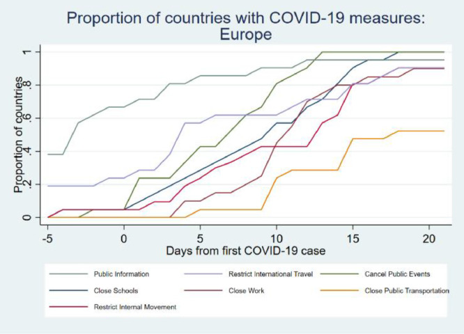
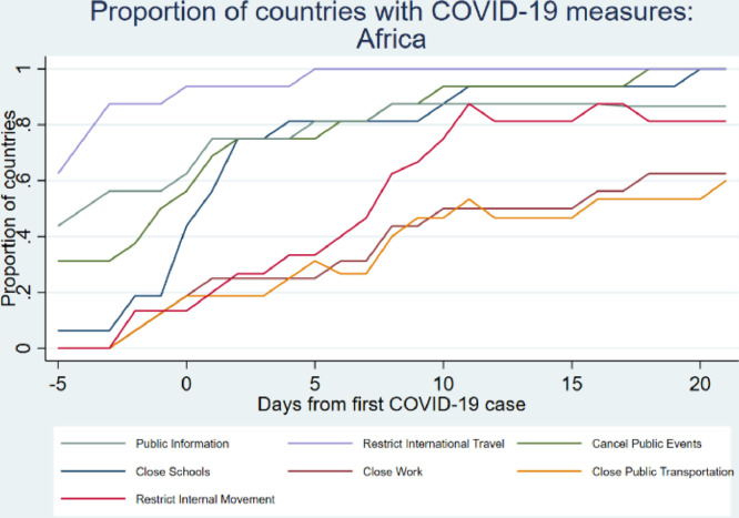
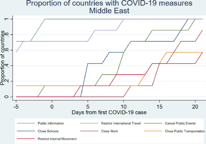
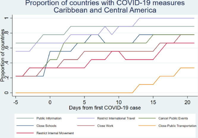
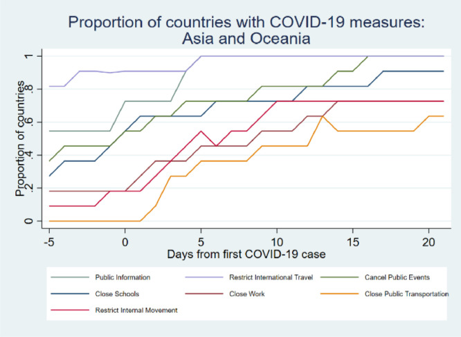
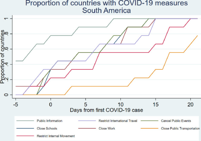
To prevent or slow down the COVID-19 epidemic countries in our sample implemented a number of policies designed to decrease the number of physical contacts between individuals in a variety of social situations, such as school, work, public events, etc. Fig. 4 represents the timeline of these restriction policies, with respect to the day of the first case, in the estimation sample. In particular, it shows the percentage of countries in our sample that have adopted each of the seven mobility restriction measures (at any stringency level, e.g. “recommended” or “required”) by each day from the onset of the COVID-19 epidemic. Day zero denotes the day when the first COVID-19 case was recorded. The mobility restriction measures include (i) provision of public information about COVID-19; (ii) restrictions on international travel; (iii) cancellation of public events; (iv) school, (v) public transport and (vi) workplace closures; and (vii) restriction of internal movement. Around 50% of countries in our sample had public information campaign and/or international travel restrictions in place at least five days before reporting their first COVID-19 case. Fifteen per cent of countries have recommended or required the cancellation of public events before the start of the pandemic. However, only a very small proportion of countries adopted any of the more restrictive policies in this initial stage. As the epidemic developed, the countries gradually adopted more policies and increased restrictions. For example, by the tenth day of the epidemic close to 90% of the countries implemented information campaigns, around 80% of the countries have restricted international travel and closed public events. By day 10 of the epidemic school closures were implemented in 70% of the countries, workplace closures and restrictions to internal movements were implemented in about 50% of the countries, and finally, about 25% of the countries implemented closures of public transportation. By the end of the sample period (day 21 from the first local COVID-19 case), almost all countries in the sample implemented information campaigns, restricted international travel, closed public events and schools. Close to 80% of them have also closed work and restricted internal movement. Finally, about 55% of the countries have also implemented some form of public transportation closure.
Fig. 4.
Proportion of countries with policy restrictions at various times after the first case.
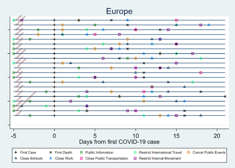
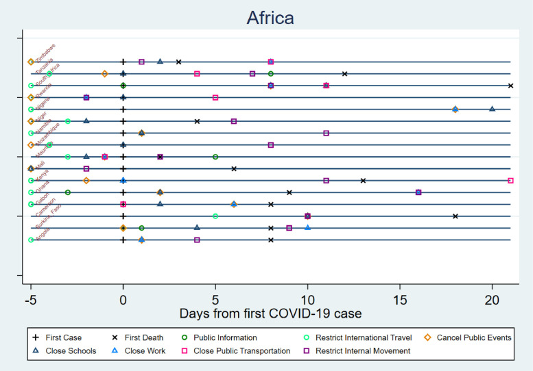
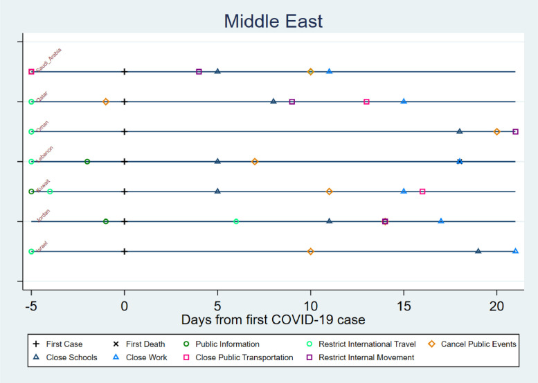
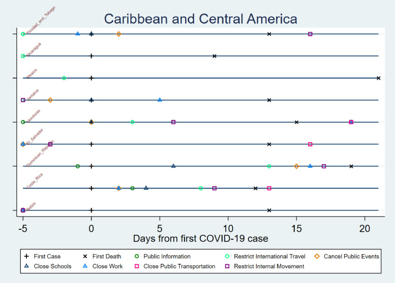
At the same time, there were notable differences in the speed of the countries’ response to COVID-19 epidemic. Figs. 5 –10 show policy timelines for 6 regions of the world in our sample. Interestingly, compared to the countries where the epidemic started later (e.g. Asian or Central American countries in our sample) the countries with the earlier start of the epidemic (such as Europe and the Middle East) were slower to adopt the COVID-19 policies (e.g. informational campaign and restrictions of international travel in Europe; or the five more restrictive policies in the Middle East). For example, about 50% of European or Middle Eastern countries in the estimation sample had implemented school closures 10 days after the start of the pandemic, while the same measure was implemented by over 50% of countries in Asia or Central America only one or two days after the first case. This might be explained by the learning process with countries where the pandemic arrives at a later date having more information on an appropriate policy response.
Fig. 6.
COVID-19 measures – Europe.
Fig. 7.
COVID-19 measures - Africa.
Fig. 8.
COVID-19 measures – Middle East.
Fig. 9.
COVID-19 measures-Caribbean and Central America.
Fig. 5.
COVID-19 measures -Asia and Oceania.
Fig. 10.
COVID-19 measures South America.
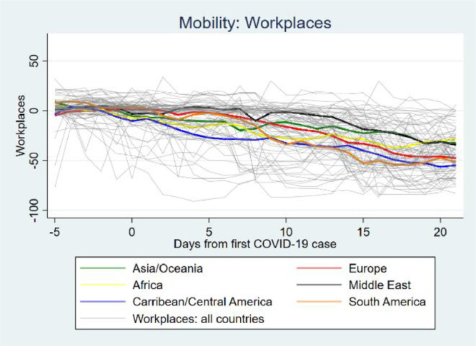
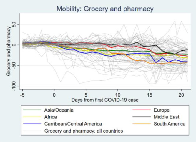
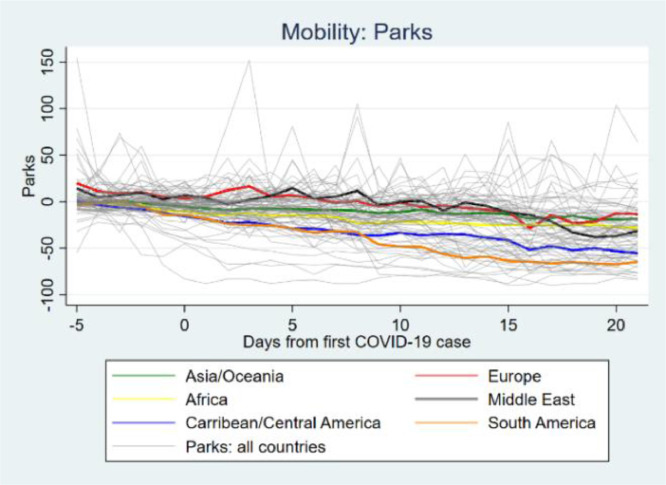
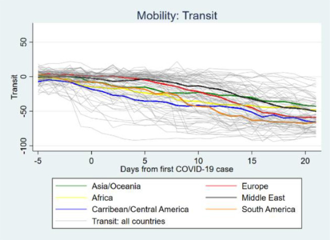
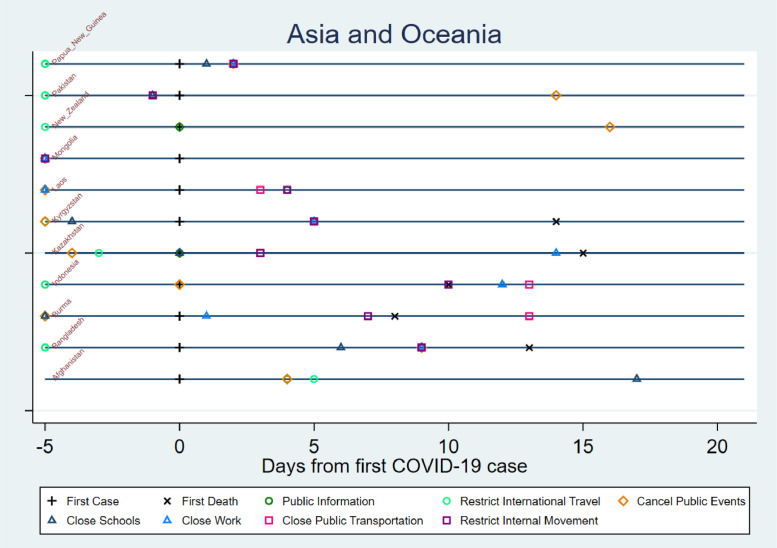
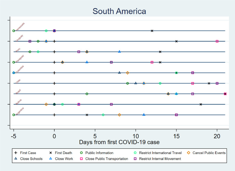
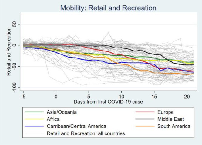
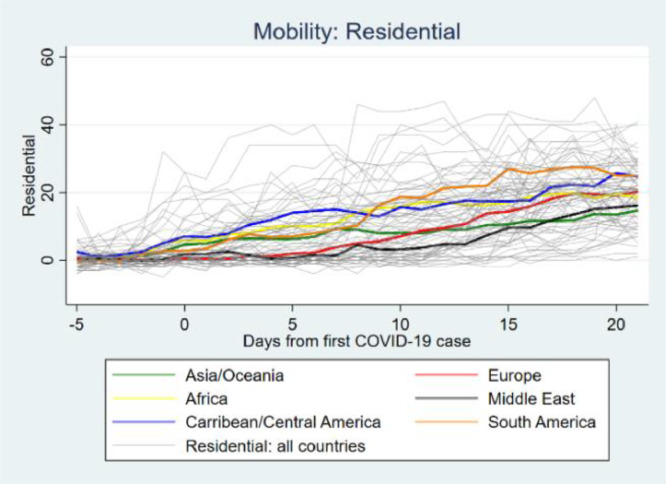
Figs. A1–A6 of the Appendix present a more disaggregated timelines of significant COVID-19 events (i.e. first case, first death, policies) for all countries in our sample, grouped by regions. Overall, countries acted at various speed in the implementation of stricter measures, and there are significant differences across the regions. Figs. 11 –16 show how mobility changed with the progression of the pandemic in all countries included in the sample (thin grey lines). It also shows the average mobility changes of countries within six regions included in the sample (coloured lines). The figures suggest that mobility drastically decreased with the increase in cases and restrictions in most countries. In particular, mobility was reduced by over 50% with respect to the baseline date (15/2/2020) after 20 days from the first case, in most countries in retail and recreational areas, parks, and public transport, while the effect was slightly lower in workplaces and around grocery shopping areas. As expected, mobility around residential areas significantly increased in the period considered. Central and South America regions show the highest decline in mobility, while the Middle East and Asian countries show moderately lower effects. These notable differences can be driven by the speed of the spread of COVID-19 cases, government responses, seasonal changes, but also other factors (e.g. geographical, cultural and economic factors that affect broad patterns of mobility in normal times and during global and national pandemics). Therefore, it is important to control for regional differences in trends in the empirical analysis.
Fig. 12.
Mobility in Workplaces.
Fig. 13.
Mobility in Grocery Stores and Pharmacies.
Fig. 14.
Mobility in Parks.
Fig. 15.
Mobility in Public Transports.
Fig. A1.
Timeline of COVID-19 events: Asia and Oceania.
Fig. A6.
Timeline of COVID-19 events: South America.
Fig. 11.
Mobility in Retail and Recreational Areas.
Fig. 16.
Mobility in Residential Areas.
4. Empirical model
As was demonstrated in the previous section, there was a large decline in all types of human mobility (except residential mobility, which actually increased) during the first 21 days of COVID-19 epidemic. Undoubtedly the restrictive policies adopted by the countries in an attempt to stop the spread of the epidemic played a significant role in these declines, as countries cancelled public events, closed public transportation, schools and workplaces, and limited internal movements in other ways. It is also plausible that in part these declines were caused by the public response to the news about the COVID-19 spread in the community, as individuals, businesses and organisations took actions to limit physical contacts with others voluntarily.
It is challenging to empirically separate the effects of the policies from those of the news about the spread of the COVID-19 cases because these events are very close in time. Our identification strategy relies on the precise and flexible modelling of the effects of restrictive COVID-19 policies and other determinants of mobility besides the COVID-19 cases and mortality, such as daily ambient temperature, days of the week and time trends (we consider several alternative specifications of these trends). The relationship between mobility and COVID-19 cases and mortality is estimated conditional on these variables, and the identification relies on the differences in the time paths of the cumulative COVID-19 cases and deaths between countries that are similar in terms of all other characteristics included in the model.
In the main analysis, we estimate three specifications which differ by modelling of the individual effects of seven COVID-19 policies discussed in the previous section (i.e. public information, international travel restrictions, cancellation of public events, and closings of schools, workplaces, public transportation and restrictions on internal movements). In the first specification, we allow for a dynamic response of mobility to policies. In the second specification, we allow for this dynamic response to differ according to the severity of the epidemic. Finally, in the third specification, we allow each policy to have a different effect on mobility depending on its stringency level (e.g. a “recommended” policy can affect the outcome differently compared to a “required” policy). In the robustness section, we examine how the effects of the COVID-19 cases and mortality on human mobility change with alternative specifications of the common trends in mobility and other characteristics of the model and estimation sample.
The first specification is given by the following model:
| (1) |
where is the percentage change in human mobility in country i, in region j and period t (we consider six types of mobility, as discussed in Section 3), relative to February 15th 2020 (the first date on which mobility data are available); is a country fixed effect; t is the number of days relative to the day of the first COVID-19 case recorded, ranging from five days before the first case to 21 days after the first case (i.e. t = 1 denotes five days before the first recorded case, t = 6 denotes the day of the first recorded COVID case, t = 27 is the last observation day, which corresponds to the day 21 after the first COVID-19 case was reported).
We include a third-degree polynomial in t, interacted with regional indicators, so that each of the six regions in our model has its own trend in time; is the average ambient daily temperature; is the date of the week fixed effects (with Sunday being the base day of the week). Functions f(.) and g(.) are flexible specifications of the cumulative number of COVID-19 cases and deaths starting from the first day of the epidemic. In particular, we specify eleven dummy variables flagging days with 1, 2, 3, 4–5, 6–10, 11–19, 20–29, 30–49, 50–99, 100–199 and at least 200 COVID-19 cases, with the baseline being days with zero COVID-19 cases recorded. For the COVID-19 deaths, the dummy variables are flagging days with 1, 2, 3, 4–5, and 6 and more deaths. The groups are chosen to have a similar number of observations.2
In model (1) we allow community mobility to adjust slowly to the policies by specifying the dynamic effects of the policies. In particular, policy variables where d = 1,…,6 are indicators equal to 1 if day t is the day from the day that policy k (k = 1, …,7) was implemented (at any stringency level)3 in country i, and is equal to zero otherwise. Similarly, are indicators for days seven and beyond after the policy implementation. Thus, model (1) allows each policy to have a different (e.g. increasing) effect in the first six days after the implementation while starting from the seventh day the effect is constrained to be the same for the remaining time that the country is in the sample. The term is a random error independent of the variables included in the model.
It is possible that mobility-restricting policies were more effective if implemented during a more advanced stage of the epidemic. Model (1) may overestimate the effect of COVID-19 cases on human mobility because it is not flexible enough to allow for such heterogeneity. To accommodate this possibility, we estimate the extended version of the model (1) by allowing the policy effects and to differ depending on the stage of the epidemic in the country on the day the policy was implemented.4 In particular, we specify the following model:
| (2) |
where is equal to 1 if country i implemented policy k on the day when COVID-19 cases count in the country i is below the median of COVID-19 cases in other countries on the day of the policy's implementation. Similarly, is equal to 1 if the country's i COVID-19 cases count was equal to or greater than the median of COVID-19 cases in other countries on the day of the policy's implementation. In the final specification we allow for different policy stringency levels (but not for dynamic policy effects which is not practical due to a small number of observations in many stringency categories) as follows:
| (3) |
Here is an indicator variable equal to one if policy k (k = 1, …,7) of stringency level s has been in place in the country i at day t. Policies differ in the stringency gradations, hence the upper limit of summation in (3) is indexed by k (i.e. ). For example, the informational campaign only has two levels (implemented or not), international travel restrictions take four levels (no measure, screening, quarantine, ban), while all other policies have three stringency levels (no measure, restriction recommended, restriction required). The distribution of stringency levels in the COVID-19 measures for the beginning, middle and the end of our sample period is presented in Table 1 . The more stringent policies (e.g. with “required” stringency) become more prevalent as the epidemic progresses and countries either increase the stringency of the existing policies or are more likely to introduce new policies at more stringent levels. All three models are estimated by fixed effects with standard errors clustered at the country level. Estimation results are presented in the next section.
Table 1.
Distribution of policy stringency categories, by days from the start of COVID-19 epidemic.
| Policy | Days from the start of COVID-19 epidemic |
|||||
|---|---|---|---|---|---|---|
| Day 0 |
Day 10 |
Day 27 |
||||
| Number of countries | % | Number of countries | % | Number of countries | % | |
| International Travel: Screening | 14 | 31.8 | 5 | 8.2 | 2 | 2.9 |
| International Travel: Quarantine | 9 | 20.5 | 11 | 18.0 | 5 | 7.1 |
| International Travel: Ban | 21 | 47.7 | 45 | 73.8 | 63 | 90.0 |
| Total | 44 | 100.0 | 61 | 100.0 | 70 | 100.0 |
| Cancel public events: recommended | 1 | 4.2 | 6 | 10.3 | 1 | 1.4 |
| Cancel public events: required | 23 | 95.8 | 52 | 89.7 | 70 | 98.6 |
| Total | 24 | 100.0 | 58 | 100.0 | 71 | 100.0 |
| School closing: recommended | 0 | 0.0 | 0 | 0.0 | 1 | 1.4 |
| School closing: required | 22 | 100.0 | 51 | 100.0 | 69 | 98.6 |
| Total | 22 | 100.0 | 51 | 100.0 | 70 | 100.0 |
| Workplace closing: recommended | 8 | 72.7 | 13 | 38.2 | 16 | 27.6 |
| Workplace closing: required | 3 | 27.3 | 21 | 61.8 | 42 | 72.4 |
| Total | 11 | 100 | 34 | 100 | 58 | 100 |
| Public transportation closing: recommended | 1 | 25.0 | 4 | 21.1 | 12 | 29.3 |
| Public transportation closing: required | 3 | 75.0 | 15 | 79.0 | 29 | 70.7 |
| Total | 4 | 100.0 | 19 | 100.0 | 41 | 100.0 |
| Restriction of internal movement: recommended | 3 | 30.0 | 10 | 24.4 | 11 | 18.6 |
| Restriction of internal movement: required | 7 | 70.0 | 31 | 75.6 | 48 | 81.4 |
| Total | 10 | 100 | 41 | 100 | 59 | 100 |
5. Results
5.1. Main results
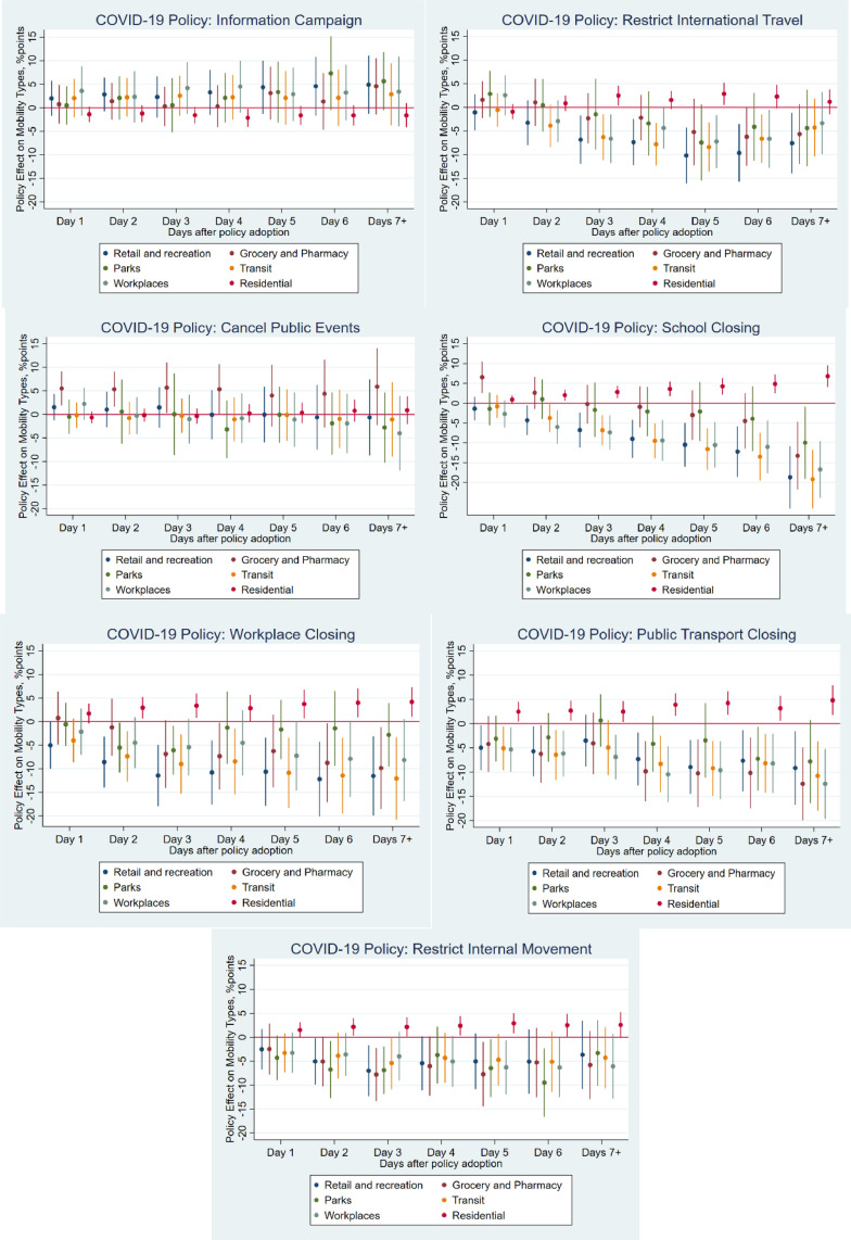
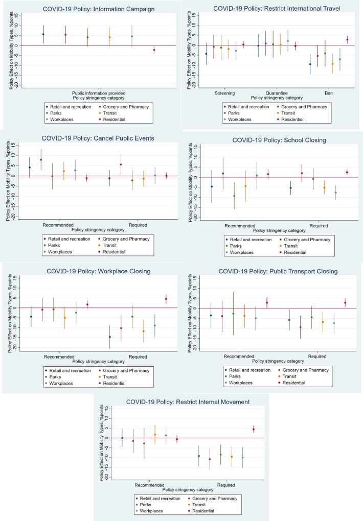
In the description of the results, we focus on the effects of COVID-19 cases and deaths estimated under alternative specifications of the policies restricting mobility as discussed in the previous section. The coefficients on the COVID-19 cases and deaths on different mobility types along with standard errors and statistical significance are presented in Table 2 . We also graphically present the effects of the policies estimated by specifications (1) and (3) on Figs. 17 −18. The policy effects from specification (2) are similar to those from specification (1).
Table 2.
Effects of COVID-19 cases and deaths on human mobility.
| (1) | (2) | (3) | (4) | (5) | (6) | (7) | (8) | (9) | |
|---|---|---|---|---|---|---|---|---|---|
| Ret&Rec | Ret&Rec | Ret&Rec | Gro&Phar | Gro&Phar | Gro&Phar | Parks | Parks | Parks | |
| Total COVID-19 cases: 1 | −2.18 | −2.09 | −1.13 | −4.68*** | −3.90** | −4.64*** | −1.84 | −2.10 | −2.06 |
| (1.41) | (1.54) | (1.42) | (1.48) | (1.60) | (1.47) | (2.00) | (2.06) | (1.98) | |
| Total COVID-19 cases: 2 | −2.91** | −4.21** | −0.47 | −6.93*** | −7.50*** | −4.84*** | −0.42 | −0.04 | 0.32 |
| (1.43) | (1.75) | (1.52) | (1.72) | (2.06) | (1.72) | (2.20) | (2.41) | (2.10) | |
| Total COVID-19 cases: 3 | −2.89 | −5.56** | −1.09 | −7.34*** | −9.07*** | −5.76** | −0.11 | −0.46 | −0.09 |
| (2.35) | (2.67) | (2.40) | (2.59) | (3.00) | (2.73) | (2.93) | (3.34) | (2.70) | |
| Total COVID-19 cases: 4–5 | −1.68 | −4.67* | −1.81 | −7.38*** | −9.86*** | −6.71*** | 1.55 | 1.70 | 0.35 |
| (2.22) | (2.66) | (2.17) | (2.33) | (2.82) | (2.30) | (3.50) | (3.95) | (3.24) | |
| Total COVID-19 cases: 6–10 | −5.07* | −9.88*** | −4.22 | −10.09*** | −14.14*** | −8.93*** | −0.36 | −0.67 | −1.68 |
| (2.84) | (3.27) | (2.59) | (2.82) | (3.17) | (2.79) | (3.72) | (4.36) | (3.14) | |
| Total COVID-19 cases: 11–19 | −6.13* | −4.68 | −5.32* | −8.28** | −7.57** | −7.65** | −0.58 | 1.89 | −1.78 |
| (3.39) | (3.48) | (2.97) | (3.27) | (3.36) | (3.20) | (3.98) | (4.81) | (3.47) | |
| Total COVID-19 cases: 20–29 | −9.23** | −7.99* | −9.30*** | −11.50*** | −11.21*** | −11.95*** | −2.29 | −0.32 | −4.49 |
| (3.94) | (4.02) | (3.50) | (3.66) | (3.85) | (3.86) | (4.82) | (5.50) | (4.21) | |
| Total COVID-19 cases: 30–49 | −10.12** | −8.74* | −9.81** | −10.15** | −7.56 | −9.82** | −1.24 | 2.61 | −3.99 |
| (4.21) | (4.53) | (3.83) | (4.34) | (4.81) | (4.74) | (5.12) | (6.48) | (4.65) | |
| Total COVID-19 cases: 50–99 | −9.92** | −8.85* | −9.81** | −9.66** | −8.25* | −10.59** | −2.31 | −1.13 | −5.40 |
| (4.61) | (4.66) | (4.00) | (4.19) | (4.57) | (4.65) | (5.32) | (6.82) | (4.61) | |
| Total COVID-19 cases: 100–199 | −12.76** | −14.95*** | −13.25*** | −11.64** | −12.39** | −13.23** | −6.53 | −4.26 | −9.14 |
| (5.17) | (5.10) | (4.66) | (4.76) | (4.74) | (5.30) | (6.05) | (7.02) | (5.82) | |
| Total COVID-19 cases: >=200 | −13.55** | −15.25*** | −13.59*** | −11.07* | −11.47** | −12.70** | −6.61 | −4.06 | −8.99 |
| (5.77) | (5.56) | (5.06) | (5.69) | (5.46) | (6.01) | (6.31) | (6.82) | (5.82) | |
| Total COVID-19 deaths: 1 | −3.64* | −3.53* | −4.48** | −2.41 | −2.13 | −3.47 | −1.81 | −1.49 | −2.32 |
| (2.05) | (2.06) | (2.14) | (1.97) | (2.01) | (2.25) | (1.84) | (1.83) | (1.99) | |
| Total COVID-19 deaths: 2 | −5.65** | −4.80* | −7.72** | −5.85* | −4.81 | −8.83** | −2.80 | −2.78 | −4.37 |
| (2.52) | (2.64) | (3.18) | (3.20) | (3.15) | (4.20) | (3.83) | (3.63) | (3.90) | |
| Total COVID-19 deaths: 3 | −3.73 | −3.22 | −4.17 | −3.64 | −2.84 | −5.19 | −2.87 | −2.97 | −3.22 |
| (3.10) | (3.01) | (3.22) | (3.17) | (3.09) | (3.58) | (3.37) | (3.32) | (3.56) | |
| Total COVID-19 deaths: 4–5 | −5.18 | −5.70 | −6.19 | −5.48 | −5.64 | −6.97 | −0.64 | −0.47 | −0.66 |
| (3.77) | (3.59) | (4.08) | (3.65) | (3.47) | (4.21) | (3.43) | (3.67) | (3.49) | |
| Total COVID-19 deaths: >=6 | −0.83 | −2.54 | −2.81 | −0.29 | −1.43 | −3.47 | −2.99 | −2.97 | −4.24 |
| (3.57) | (3.48) | (4.11) | (4.09) | (4.08) | (5.22) | (5.37) | (5.39) | (6.25) | |
| Seven COVID-19 policy measures with dynamic effects | Yes | Yes | Yes | ||||||
| Seven COVID-19 policy measures with dynamic effects and interactions with the stage of the epidemic | Yes | Yes | Yes | ||||||
| Seven COVID-19 policies disaggregated by stringency levels | Yes | Yes | Yes | ||||||
| Constant | 86.81*** | 87.32*** | 87.26*** | 88.32*** | 88.47*** | 85.57*** | 71.58*** | 72.14*** | 69.53*** |
| (3.37) | (3.32) | (3.62) | (3.37) | (3.29) | (4.13) | (5.01) | (4.99) | (5.05) | |
| Observations | 1971 | 1971 | 1909 | 1971 | 1971 | 1909 | 1971 | 1971 | 1909 |
| Adjusted R-squared | 0.806 | 0.811 | 0.810 | 0.603 | 0.609 | 0.581 | 0.500 | 0.499 | 0.516 |
| (10) | (11) | (12) | (13) | (14) | (15) | (16) | (17) | (18) | |
| Transit | Transit | Transit | Work | Work | Work | Resid | Resid | Resid | |
| Total COVID-19 cases: 1 | −2.41* | −2.95** | −1.61 | −2.37 | −2.42 | −1.52 | 1.03* | 1.05* | 0.67 |
| (1.32) | (1.47) | (1.35) | (1.60) | (1.69) | (1.67) | (0.53) | (0.55) | (0.55) | |
| Total COVID-19 cases: 2 | −2.85* | −3.53* | −0.42 | −5.34** | −5.27** | −2.74 | 1.18* | 1.12 | 0.15 |
| (1.57) | (1.80) | (1.70) | (2.12) | (2.40) | (2.04) | (0.62) | (0.81) | (0.56) | |
| Total COVID-19 cases: 3 | −3.28 | −4.74* | −1.28 | −6.64** | −7.74** | −4.52 | 1.79* | 2.10* | 0.88 |
| (2.30) | (2.38) | (2.40) | (2.92) | (3.11) | (2.91) | (0.99) | (1.13) | (0.98) | |
| Total COVID-19 cases: 4–5 | −2.45 | −4.37* | −2.70 | −5.87** | −7.82** | −5.39** | 1.55* | 2.11* | 1.52* |
| (2.10) | (2.51) | (2.14) | (2.64) | (3.03) | (2.46) | (0.87) | (1.10) | (0.81) | |
| Total COVID-19 cases: 6–10 | −4.96** | −8.46*** | −3.83 | −7.78** | −11.73*** | −5.89** | 2.06** | 3.06** | 1.43 |
| (2.49) | (2.89) | (2.39) | (3.14) | (3.35) | (2.91) | (1.00) | (1.19) | (0.93) | |
| Total COVID-19 cases: 11–19 | −5.72* | −4.43 | −4.68* | −7.46** | −5.44 | −5.83* | 1.89* | 1.43 | 1.33 |
| (2.92) | (3.22) | (2.67) | (3.42) | (3.68) | (2.97) | (1.12) | (1.29) | (1.06) | |
| Total COVID-19 cases: 20–29 | −8.08** | −6.77* | −7.55** | −9.31** | −7.48* | −8.01** | 2.47* | 2.13 | 2.26* |
| (3.42) | (3.76) | (3.26) | (4.04) | (4.29) | (3.57) | (1.31) | (1.49) | (1.27) | |
| Total COVID-19 cases: 30–49 | −10.71*** | −9.42** | −9.79*** | −11.44** | −8.92* | −9.81** | 3.25** | 2.83* | 2.87** |
| (3.95) | (4.21) | (3.66) | (4.33) | (4.61) | (3.75) | (1.48) | (1.66) | (1.40) | |
| Total COVID-19 cases: 50–99 | −10.58** | −9.02** | −9.91** | −7.91* | −5.70 | −6.57* | 2.57* | 2.63 | 2.34 |
| (4.24) | (4.33) | (3.80) | (4.51) | (4.72) | (3.93) | (1.52) | (1.65) | (1.43) | |
| Total COVID-19 cases: 100–199 | −12.23*** | −13.90*** | −12.13*** | −9.38* | −9.72* | −8.84* | 3.10* | 4.49** | 3.24* |
| (4.60) | (4.84) | (4.31) | (5.07) | (5.25) | (4.56) | (1.81) | (1.79) | (1.74) | |
| Total COVID-19 cases: >=200 | −14.11*** | −15.39*** | −13.78*** | −9.50 | −9.49 | −8.17 | 3.76* | 5.04** | 3.63* |
| (5.17) | (5.43) | (4.49) | (6.02) | (6.13) | (5.12) | (2.14) | (2.07) | (1.97) | |
| Total COVID-19 deaths: 1 | −1.48 | −1.53 | −1.89 | −2.08 | −1.74 | −2.44 | 1.22 | 1.11 | 1.25 |
| (2.04) | (2.02) | (1.99) | (2.09) | (2.13) | (2.12) | (0.84) | (0.84) | (0.85) | |
| Total COVID-19 deaths: 2 | −3.03 | −2.61 | −4.68 | −4.56 | −3.55 | −6.16* | 2.15* | 1.90* | 2.81** |
| (2.43) | (2.51) | (3.04) | (2.94) | (2.90) | (3.54) | (1.15) | (1.14) | (1.40) | |
| Total COVID-19 deaths: 3 | −2.63 | −2.21 | −2.65 | −1.48 | −0.39 | −1.74 | 1.43 | 1.19 | 1.39 |
| (2.95) | (2.82) | (2.84) | (3.21) | (3.05) | (3.28) | (1.19) | (1.15) | (1.16) | |
| Total COVID-19 deaths: 4–5 | −4.33 | −4.76 | −5.41 | −5.62* | −5.86* | −6.95* | 2.25 | 2.53* | 2.60* |
| (3.55) | (3.31) | (3.70) | (3.23) | (3.09) | (3.56) | (1.37) | (1.29) | (1.35) | |
| Total COVID-19 deaths: >=6 | −0.76 | −2.36 | −3.33 | −2.55 | −3.56 | −4.62 | 1.28 | 1.93 | 2.49* |
| (3.49) | (3.24) | (3.70) | (3.31) | (3.21) | (3.74) | (1.37) | (1.30) | (1.44) | |
| Seven COVID-19 policy measures with dynamic effects | Yes | Yes | Yes | ||||||
| Seven COVID-19 policy measures with dynamic effects and interactions with the stage of the epidemic | Yes | Yes | Yes | ||||||
| Seven COVID-19 policies disaggregated by stringency levels | Yes | Yes | Yes | ||||||
| Constant | 86.44*** | 86.74*** | 87.46*** | 98.94*** | 99.22*** | 100.72*** | 102.21*** | 101.94*** | 102.12*** |
| (3.04) | (3.06) | (3.15) | (3.99) | (4.01) | (4.26) | (1.52) | (1.52) | (1.55) | |
| Observations | 1971 | 1971 | 1909 | 1971 | 1971 | 1909 | 1961 | 1961 | 1899 |
| Adjusted R-squared | 0.836 | 0.840 | 0.835 | 0.717 | 0.721 | 0.720 | 0.783 | 0.786 | 0.786 |
All models include country fixed effects, cubic polynomial in ambient temperature, days of the week fixed effects and regional cubic polynomial trends in the number of days from the first COVID-19 case. Standard errors clustered at the country level are in parentheses. Asterisks denote statistical significance: * p<0.10, ** p<0.05, *** p<0.01.
Fig. 17.
Effects of policies on mobility, model (1).
The results in Table 2 suggest that COVID-19 cases have statistically and economically significant effects on mobility, even conditional on the flexible specification of the effects of policies and common trends. The three models produce quantitatively similar effects of COVID-19 cases. Compared to model (1), model (2) suggests somewhat larger effects of cases, while model (3) suggests smaller effects, especially for the first few cases, for some mobility types (retail and recreation, transit, workplaces and residential mobility). But even in the model (3) the retail and recreation mobility starts to decline once the country reaches 11 or more COVID-19 cases. Relative to the pre-epidemic mobility, cases 11–19 are associated with 5% decline, further increases in cases are associated with increasing declines until the threshold of 100–200 cases associated with 13% of mobility decline is reached. Additional cases beyond two hundred do not seem to bring about further decreases in mobility,5 with the coefficient on the dummy variable flagging days with 200 and more being equal to −13.59%. Mobility related to groceries and pharmacies shopping and transit is affected very similarly by cases, whereas workplace mobility seems to be affected less, with the coefficients on cases being smaller in absolute value and of a lower statistical significance. It should be noted that the coefficients on the same variable may not be directly comparable across the types of mobility because they depend on the absolute levels of mobility.6 Keeping this caveat in mind, one interpretation of the lower effects of cases on workplaces mobility is that presumably, people have less discretion over work-related travel than over personal travel for the purposes of shopping and recreation. Mobility related to travel to and around parks is not affected by cases, whereas residential mobility is affected positively, but the effects are small in absolute value and of low statistical significance (e.g. model (3) suggests a statistically significant increase of 3.63 percentage points when COVID-19 cases count reaches 200 or more). In the Robustness section, we show that these effects change little when more flexible model specifications are used.
COVID-19-related deaths have a modest negative effect on some mobility types in some models. In particular, the occurrence of the first death decreases retail and recreation mobility by 4.48% (results are similar across the three models). The second COVID-19 death decreases retail and recreation mobility by 7.72% (similar results across the three models), groceries and pharmacy mobility by 5.85% in the model (1) and by 8.83% in the model (2), and work-related mobility by 6.16% (in model 3 only). The second COVID-19 death also increases residential mobility by about 2% (the results are similar across the three models). COVID-19 deaths numbers greater than two do not have statistically significant effects on mobility, except for the indicator of 4–5 deaths which decreases workplaces mobility by about 6% in all three models and increase residential mobility by about 2.5% in models 2 and 3.
Overall, the results suggest that COVID-19 cases have had a long-lasting moderate effect on mobility that is independent of the social distancing policies implemented by the government. In the first three weeks of the epidemic, most types of mobility show a gradual decline until a maximum reduction of about 10–15 percentage points as the accumulated count of cases reached 100 and beyond. COVID-19 related deaths, on the other hand, seem to have a short-lived effect, with the first few cases temporarily reduce mobility by several percentage points, and subsequent deaths having no statistically significant impact on mobility.
The effects of the policies are presented in Figs. 17 and 18 . Fig. 17, where the seven panels show the coefficients from the models (1) and (3) for each mobility type. Results from the model (2) are similar to those from the model (1) and are available upon request. Interestingly, both models imply that the effects of the information campaigns on all types of mobility apart from residential is positive. This effect is statistically significant for retail and groceries and pharmacy-related mobility. This pattern is most likely due to forward-looking shopping behaviour in preparation for the coming mobility restrictions and is consistent with widely documented instances of “panic buying” and the resulting shortage at the start of the epidemic. Cancellation of public events seems to not affect mobility, except for some positive effects on retail, recreation, groceries and pharmacies mobility, which again can be explained by individuals stocking up on essential goods in expectations of the unfolding of an epidemic.
Fig. 18.
Effects of policies on mobility, model (3).
Policies that are more restrictive in nature have significant negative effects on mobility. Restrictions on international travel, school closing, workplaces closing, public transportation closings and restrictions on internal movements each have large negative and statistically significant effects on mobility of about 5–15 percentage points, depending on the type of mobility and the model. Model (1) suggest that the polices become more effective the longer they have been in place, whereas model (3) suggests that, for most mobility types, higher stringency level (e.g. required vs recommended) lead to larger reductions in mobility. These policies also lead to an increase in residential mobility of up to 7 percentage points.
To sum up these findings, the combined effect of the policies can explain up to 50 percentage points of permanent reductions in mobility, whereas information about COVID-19 cases can account for up to 15 percentage points of the mobility reduction. One can conclude based on these results that the information about the state of the epidemic, proxied by the number of COVID-19 cases, has a significant effect in restricting mobility. This effect is independent of the effect of policy restrictions but moderate in magnitude. Overall, our results suggest that the significant reduction in social interactions needed to slow down the spread of the virus would not have been achieved by relying on community responses alone. This conclusion is also borne out by the more recent evidence of the emerging second waves of infections in various countries after the social distancing measures are relaxed. At the same time, the existence of a significant community response that is independent of the government policies implies that one cannot expect that economically relevant activities associated with the types of mobility studied in the paper would return to normal pre-crisis level after social distancing mandates are lifted. Public perceptions about the risk of infection will continue to play a significant role in the pace of recovery until eradication of the virus or arrival of a vaccine.
5.2. Robustness checks
We conduct several additional analyses to check if alternative specifications will decrease the size and statistical significance of the effects of COVID-19 cases and mortality on human mobility. The estimates of the coefficients on COVID-19 cases and mortality are presented in Tables A1 –A6 of the Appendix.7 First, in each model discussed in the previous sections, we replace the region-specific cubic trend in the day from the start of the epidemic with the region-specific cubic trend in the calendar day. The estimated effects of policies and COVID-19 cases and mortality are presented in Appendix Table A1 and are quite similar to those reported in Table 2. A notable difference is that this model suggests somewhat smaller effects of most policies and larger effects of the first COVID-19 cases (up to 10) on most mobility types.
Table A1.
Effect of COVID-19 cases and mortality on human mobility: calendar days regional trends, model (1).
| (1) | (2) | (3) | (4) | (5) | (6) | |
|---|---|---|---|---|---|---|
| Ret&Rec | Gro&Phar | Parks | Transit | Work | Resid | |
| Total COVID-19 cases: 1 | −4.87*** | −5.63*** | −5.41** | −3.81** | −2.25 | 1.68*** |
| (1.75) | (1.56) | (2.22) | (1.46) | (1.45) | (0.58) | |
| Total COVID-19 cases: 2 | −5.08** | −7.98*** | −4.78** | −3.67** | −4.50** | 1.72** |
| (1.93) | (2.00) | (2.28) | (1.79) | (1.86) | (0.66) | |
| Total COVID-19 cases: 3 | −4.98* | −7.80** | −4.20 | −3.83 | −5.50** | 2.11** |
| (2.96) | (2.95) | (2.79) | (2.39) | (2.57) | (1.00) | |
| Total COVID-19 cases: 4–5 | −3.75 | −7.72*** | −2.46 | −2.88 | −4.01* | 1.65* |
| (2.40) | (2.50) | (3.34) | (2.04) | (2.31) | (0.84) | |
| Total COVID-19 cases: 6–10 | −6.76** | −10.49*** | −4.30 | −5.13** | −6.29** | 2.14** |
| (2.79) | (2.79) | (3.53) | (2.33) | (2.70) | (0.93) | |
| Total COVID-19 cases: 11–19 | −6.94** | −8.78*** | −5.14 | −5.32* | −5.55* | 1.79* |
| (3.31) | (3.31) | (3.67) | (2.79) | (3.07) | (1.00) | |
| Total COVID-19 cases: 20–29 | −9.78** | −11.95*** | −7.03 | −7.12** | −7.20** | 2.25* |
| (3.89) | (3.62) | (4.35) | (3.28) | (3.54) | (1.18) | |
| Total COVID-19 cases: 30–49 | −10.68** | −10.89** | −6.54 | −9.77*** | −9.58** | 2.96** |
| (4.07) | (4.18) | (4.74) | (3.63) | (3.79) | (1.31) | |
| Total COVID-19 cases: 50–99 | −10.16** | −10.51** | −7.38 | −9.39** | −6.13 | 2.16 |
| (4.42) | (4.11) | (4.77) | (3.89) | (3.91) | (1.32) | |
| Total COVID-19 cases: | −13.08*** | −12.67*** | −11.30** | −10.97** | −7.79* | 2.75* |
| 100–199 | (4.87) | (4.51) | (5.56) | (4.22) | (4.51) | (1.64) |
| Total COVID-19 cases: >=200 | −13.43** | −12.47** | −9.31 | −12.42** | −8.14 | 3.18* |
| (5.55) | (5.48) | (6.00) | (4.77) | (5.36) | (1.87) | |
| Total COVID-19 deaths: 1 | −1.20 | −0.24 | −1.78 | 0.59 | 0.10 | 0.39 |
| (1.97) | (1.95) | (1.81) | (1.90) | (1.86) | (0.82) | |
| Total COVID-19 deaths: 2 | −4.78* | −4.09 | −2.88 | −2.78 | −4.33 | 2.16** |
| (2.65) | (3.13) | (3.70) | (2.15) | (2.65) | (1.04) | |
| Total COVID-19 deaths: 3 | −1.58 | −1.08 | −2.04 | −1.22 | 0.29 | 0.85 |
| (2.97) | (3.08) | (3.38) | (2.70) | (2.86) | (1.06) | |
| Total COVID-19 deaths: 4–5 | −3.93 | −4.11 | −1.94 | −3.70 | −4.35 | 1.88 |
| (4.01) | (3.85) | (3.69) | (3.54) | (3.48) | (1.32) | |
| Total COVID-19 deaths: >=6 | 2.09 | 4.42 | 0.99 | 0.65 | 0.30 | 0.43 |
| (3.24) | (3.31) | (4.72) | (3.16) | (3.06) | (1.18) | |
| Seven COVID-19 policy measures with dynamic effects | Yes | Yes | Yes | Yes | Yes | Yes |
| Observations | 1971 | 1971 | 1971 | 1971 | 1971 | 1961 |
| Adjusted R-squared | 0.824 | 0.629 | 0.514 | 0.855 | 0.751 | 0.803 |
| Effect of COVID-19 cases and mortality on human mobility: calendar days regional trends, model (2) | ||||||
| Total COVID-19 cases: 1 | −4.62** | −4.79*** | −5.70** | −4.35*** | −2.33 | 1.72*** |
| (1.97) | (1.73) | (2.35) | (1.60) | (1.68) | (0.64) | |
| Total COVID-19 cases: 2 | −6.51*** | −8.98*** | −5.30** | −4.50** | −4.71** | 1.73** |
| (2.01) | (2.07) | (2.32) | (1.76) | (2.05) | (0.72) | |
| Total COVID-19 cases: 3 | −7.28** | −9.36*** | −5.29* | −5.10** | −6.24** | 2.30** |
| (3.11) | (3.14) | (3.09) | (2.35) | (2.71) | (1.06) | |
| Total COVID-19 cases: 4–5 | −6.10** | −10.11*** | −2.96 | −4.36** | −5.41** | 1.98** |
| (2.60) | (2.69) | (3.56) | (2.13) | (2.55) | (0.94) | |
| Total COVID-19 cases: 6–10 | −9.88*** | −13.52*** | −4.78 | −7.19*** | −8.43*** | 2.47** |
| (3.21) | (3.00) | (4.01) | (2.49) | (2.89) | (1.01) | |
| Total COVID-19 cases: 11–19 | −6.15* | −9.86*** | −3.84 | −4.28* | −4.87* | 1.50 |
| (3.15) | (3.04) | (4.23) | (2.50) | (2.79) | (0.96) | |
| Total COVID-19 cases: 20–29 | −8.98** | −13.39*** | −6.25 | −5.89* | −6.53* | 2.00* |
| (3.73) | (3.39) | (4.85) | (3.05) | (3.30) | (1.14) | |
| Total COVID-19 cases: 30–49 | −10.15** | −10.74** | −5.21 | −8.38** | −8.69** | 2.57** |
| (4.28) | (4.61) | (5.85) | (3.23) | (3.77) | (1.29) | |
| Total COVID-19 cases: 50–99 | −9.24** | −10.75** | −7.65 | −7.21** | −4.69 | 2.03 |
| (4.33) | (4.29) | (5.82) | (3.40) | (3.87) | (1.27) | |
| Total COVID-19 cases: | −14.67*** | −15.31*** | −13.00* | −11.30*** | −8.10* | 3.81** |
| 100–199 | (4.75) | (4.43) | (6.83) | (4.01) | (4.46) | (1.53) |
| Total COVID-19 cases: >=200 | −14.61*** | −14.74*** | −10.61 | −12.39*** | −8.21 | 4.18** |
| (5.15) | (5.22) | (6.89) | (4.48) | (5.27) | (1.74) | |
| Total COVID-19 deaths: 1 | −1.29 | −0.11 | −1.64 | 0.43 | 0.25 | 0.29 |
| (2.01) | (1.98) | (1.88) | (1.86) | (1.92) | (0.80) | |
| Total COVID-19 deaths: 2 | −4.54 | −3.62 | −3.10 | −2.75 | −3.89 | 2.09** |
| (2.74) | (3.13) | (3.56) | (2.22) | (2.67) | (1.04) | |
| Total COVID-19 deaths: 3 | −1.65 | −0.72 | −2.16 | −1.11 | 0.80 | 0.70 |
| (2.89) | (3.01) | (3.35) | (2.60) | (2.74) | (1.03) | |
| Total COVID-19 deaths: 4–5 | −4.93 | −4.77 | −2.44 | −4.40 | −4.83 | 2.25* |
| (3.76) | (3.53) | (3.84) | (3.23) | (3.22) | (1.24) | |
| Total COVID-19 deaths: >=6 | 0.16 | 2.85 | −0.20 | −0.86 | −0.72 | 1.03 |
| (3.02) | (3.21) | (4.86) | (2.92) | (2.91) | (1.12) | |
| Seven COVID-19 policy measures with dynamic effects and interactions with the stage of the epidemic | Yes | Yes | Yes | Yes | Yes | Yes |
| Observations | 1971 | 1971 | 1971 | 1971 | 1971 | 1961 |
| Adjusted R-squared | 0.826 | 0.634 | 0.511 | 0.857 | 0.751 | 0.804 |
| Effect of COVID-19 cases and mortality on human mobility: calendar days regional trends, model (3) | ||||||
| Total COVID-19 cases: 1 | −4.68*** | −6.87*** | −5.67** | −3.79** | −1.90 | 1.63*** |
| (1.72) | (1.66) | (2.23) | (1.63) | (1.56) | (0.60) | |
| Total COVID-19 cases: 2 | −4.28** | −7.89*** | −4.73* | −2.76 | −3.12* | 1.34** |
| (2.00) | (2.18) | (2.49) | (1.95) | (1.78) | (0.62) | |
| Total COVID-19 cases: 3 | −4.31 | −7.72** | −4.14 | −2.87 | −4.03* | 1.61* |
| (2.74) | (3.00) | (2.97) | (2.26) | (2.28) | (0.89) | |
| Total COVID-19 cases: 4–5 | −4.89** | −8.95*** | −3.69 | −4.13** | −4.40** | 2.07*** |
| (2.34) | (2.60) | (3.40) | (2.03) | (2.16) | (0.77) | |
| Total COVID-19 cases: 6–10 | −6.78** | −10.92*** | −5.45 | −4.89** | −5.04** | 1.91** |
| (2.58) | (2.83) | (3.56) | (2.18) | (2.44) | (0.88) | |
| Total COVID-19 cases: 11–19 | −6.91** | −9.41*** | −5.97 | −4.86** | −4.24 | 1.54* |
| (2.80) | (3.14) | (3.76) | (2.39) | (2.54) | (0.86) | |
| Total COVID-19 cases: 20–29 | −10.40*** | −13.55*** | −8.71** | −7.06** | −6.06* | 2.25** |
| (3.40) | (3.64) | (4.34) | (2.98) | (3.10) | (1.05) | |
| Total COVID-19 cases: 30–49 | −10.39*** | −11.11** | −8.68* | −8.65*** | −7.41** | 2.60** |
| (3.59) | (4.32) | (4.78) | (3.25) | (3.25) | (1.15) | |
| Total COVID-19 cases: 50–99 | −9.99*** | −11.77*** | −9.54** | −8.40** | −3.96 | 1.84 |
| (3.74) | (4.01) | (4.70) | (3.42) | (3.42) | (1.18) | |
| Total COVID-19 cases: | −12.77*** | −13.77*** | −12.89** | −9.86** | −5.61 | 2.50* |
| 100–199 | (4.22) | (4.48) | (5.65) | (3.76) | (3.97) | (1.50) |
| Total COVID-19 cases: >=200 | −12.56** | −13.31** | −11.20* | −10.81** | −4.74 | 2.54 |
| (4.88) | (5.48) | (5.98) | (4.13) | (4.61) | (1.73) | |
| Total COVID-19 deaths: 1 | −1.56 | −0.37 | −1.82 | 1.00 | 0.48 | 0.22 |
| (2.01) | (2.08) | (1.97) | (1.77) | (1.89) | (0.82) | |
| Total COVID-19 deaths: 2 | −5.80** | −6.00 | −3.88 | −3.04 | −4.81* | 2.35** |
| (2.83) | (3.68) | (3.64) | (2.31) | (2.79) | (1.11) | |
| Total COVID-19 deaths: 3 | −1.34 | −1.35 | −1.73 | −0.23 | 0.92 | 0.51 |
| (2.79) | (3.00) | (3.24) | (2.35) | (2.76) | (0.93) | |
| Total COVID-19 deaths: 4–5 | −4.07 | −4.13 | −0.92 | −3.52 | −4.78 | 1.92 |
| (3.97) | (3.96) | (3.81) | (3.48) | (3.67) | (1.29) | |
| Total COVID-19 deaths: >=6 | 1.41 | 3.48 | 1.48 | −0.42 | −0.81 | 1.10 |
| (3.28) | (3.66) | (4.96) | (3.06) | (3.18) | (1.12) | |
| Seven COVID-19 policies disaggregated by stringency levels | Yes | Yes | Yes | Yes | Yes | Yes |
| Observations | 1909 | 1909 | 1909 | 1909 | 1909 | 1899 |
| Adjusted R-squared | 0.829 | 0.619 | 0.537 | 0.858 | 0.760 | 0.811 |
All models include country fixed effects, cubic polynomial in ambient temperature, days of the week fixed effects and regional cubic polinomial trends in calendar days.
Standard errors clustered at the country level are in parentheses.
Asterisks denote statistical significance: * p<0.10, ** p<0.05, *** p<0.01.
Table A6.
Effect of COVID-19 cases and mortality on human mobility by country size, model (1).
| Quartile 1 (Population <=4.88 mln) |
Quartile 2 (Population between 4.88mln and 9.95 mln) |
|||||||||||
|---|---|---|---|---|---|---|---|---|---|---|---|---|
| (1) | (2) | (3) | (4) | (5) | (6) | (1) | (2) | (3) | (4) | (5) | (6) | |
| Ret&Rec | Gro&Phar | Parks | Transit | Work | Resid | Ret&Rec | Gro&Phar | Parks | Transit | Work | Resid | |
| Total COVID-19 cases: 1 | −4.60 | −7.70** | −3.79 | −4.94 | −3.95 | 1.50 | −4.10 | −5.47*** | −2.67 | −3.91** | −3.48 | 1.31 |
| (3.80) | (3.42) | (5.01) | (3.17) | (3.34) | (1.34) | (2.72) | (2.06) | (2.93) | (1.83) | (2.64) | (0.93) | |
| Total COVID-19 cases: 2 | −0.80 | −7.35*** | −1.43 | −1.60 | −3.60 | 1.35 | −2.41 | −7.13 | 0.45 | −2.54 | −5.00 | 1.48 |
| (2.27) | (2.43) | (3.28) | (2.34) | (2.71) | (1.07) | (4.26) | (4.32) | (4.01) | (4.20) | (3.89) | (1.44) | |
| Total COVID-19 cases: 3 | −4.24 | −9.69** | −2.09 | −6.24* | −8.51* | 2.76 | −8.74 | −9.56 | −3.53 | −8.15 | −11.45** | 3.43* |
| (4.35) | (4.34) | (4.02) | (3.57) | (4.52) | (1.77) | (5.73) | (7.02) | (5.60) | (5.05) | (5.14) | (2.03) | |
| Total COVID-19 cases: 4–5 | −7.56** | −13.11*** | −9.54** | −8.24** | −11.69*** | 3.64*** | −4.19 | −9.00** | 3.96 | −5.19 | −10.96*** | 2.88** |
| (3.39) | (3.99) | (4.52) | (3.35) | (3.78) | (1.29) | (3.58) | (4.16) | (4.61) | (3.43) | (3.76) | (1.39) | |
| Total COVID-19 cases: 6–10 | −9.44** | −12.73*** | −4.64 | −9.33*** | −8.61** | 3.16** | −9.97** | −12.28*** | −0.90 | −11.12*** | −16.54*** | 4.13*** |
| (3.91) | (3.99) | (4.95) | (3.48) | (3.68) | (1.21) | (3.92) | (3.75) | (5.16) | (3.48) | (5.12) | (1.50) | |
| Total COVID-19 cases: 11–19 | −12.13** | −14.76*** | −5.45 | −11.40** | −11.52** | 4.14*** | −13.93*** | −14.58*** | −2.02 | −15.07*** | −16.87*** | 4.70*** |
| (4.65) | (4.43) | (6.02) | (4.36) | (4.55) | (1.53) | (4.70) | (4.83) | (5.27) | (4.35) | (5.00) | (1.62) | |
| Total COVID-19 cases: 20–29 | −14.75*** | −14.05*** | −3.74 | −13.61*** | −9.79** | 3.80** | −14.14** | −19.72*** | −0.80 | −13.09** | −16.30*** | 4.24** |
| (4.94) | (4.53) | (7.01) | (3.97) | (4.62) | (1.69) | (6.13) | (7.04) | (6.48) | (5.50) | (5.45) | (1.95) | |
| Total COVID-19 cases: 30–49 | −13.57** | −15.27** | −2.09 | −13.52*** | −10.57** | 3.82** | −14.39*** | −14.26** | −1.87 | −14.92*** | −17.95*** | 5.35*** |
| (5.70) | (6.11) | (7.32) | (4.96) | (5.20) | (1.78) | (5.36) | (5.71) | (5.94) | (4.95) | (5.22) | (2.01) | |
| Total COVID-19 cases: 50–99 | −16.11*** | −14.36*** | −4.91 | −16.44*** | −9.04* | 4.09** | −16.91*** | −17.44*** | −5.86 | −16.13*** | −16.68*** | 5.30*** |
| (5.59) | (5.39) | (6.85) | (4.69) | (5.32) | (1.90) | (5.86) | (5.92) | (6.40) | (5.52) | (5.46) | (1.87) | |
| Total COVID-19 cases: | −18.40*** | −19.98*** | −4.87 | −16.81*** | −14.09** | 5.10** | −15.90** | −17.79** | −14.65** | −16.44*** | −13.73** | 4.75** |
| 100–199 | (6.23) | (5.97) | (7.53) | (5.00) | (5.91) | (2.21) | (6.65) | (7.09) | (7.21) | (5.84) | (6.13) | (2.34) |
| Total COVID-19 cases: >=200 | −18.51** | −17.31** | 1.22 | −14.17** | −10.22 | 4.77 | −14.56** | −14.45* | −1.00 | −17.47*** | −14.59** | 5.00** |
| (7.32) | (7.94) | (7.97) | (5.94) | (7.27) | (2.97) | (6.56) | (7.36) | (10.05) | (5.88) | (6.26) | (2.38) | |
| Total COVID-19 deaths: 1 | −2.42 | −3.46 | −3.96 | −2.00 | −3.45 | 1.39 | −4.37 | −1.11 | −0.42 | −2.49 | −1.81 | 0.26 |
| (3.34) | (3.20) | (3.50) | (3.26) | (3.67) | (1.31) | (3.33) | (4.08) | (3.53) | (2.62) | (2.97) | (1.11) | |
| Total COVID-19 deaths: 2 | −4.76 | −9.43* | −2.64 | −6.60 | −10.76** | 3.94** | −3.12 | −0.53 | −0.41 | 0.45 | 0.51 | 0.08 |
| (4.12) | (5.18) | (9.21) | (4.14) | (5.14) | (1.95) | (3.41) | (4.33) | (4.83) | (3.21) | (3.24) | (1.21) | |
| Total COVID-19 deaths: 3 | −2.09 | −2.35 | −5.08 | −0.75 | −4.78 | 1.90 | −4.64 | −4.28 | −4.13 | −3.93 | −1.71 | 1.83 |
| (5.47) | (5.52) | (6.19) | (4.45) | (5.46) | (1.91) | (5.74) | (5.54) | (9.15) | (4.39) | (4.17) | (1.89) | |
| Total COVID-19 deaths: 4–5 | −1.97 | −2.58 | −10.57 | −0.61 | −4.77 | 1.71 | 1.41 | 2.17 | 14.81 | 3.23 | 1.03 | 0.04 |
| (6.50) | (9.27) | (7.23) | (4.80) | (5.34) | (1.86) | (2.89) | (3.86) | (10.76) | (3.62) | (3.64) | (1.54) | |
| Total COVID-19 deaths: >=6 | −3.84 | 0.40 | −12.34** | −3.16 | −5.73 | −0.36 | 2.30 | 6.65 | 11.29 | 7.10 | 2.45 | −0.00 |
| (5.65) | (6.29) | (4.91) | (5.88) | (5.55) | (2.59) | (6.02) | (4.59) | (12.14) | (5.03) | (4.26) | (2.12) | |
| Seven COVID-19 policy measures with dynamic effects | Yes | Yes | Yes | Yes | Yes | Yes | Yes | Yes | Yes | Yes | Yes | Yes |
| Observations | 1971 | 1971 | 1971 | 1971 | 1971 | 1961 | 1971 | 1971 | 1971 | 1971 | 1971 | 1961 |
| Adjusted R-squared | 0.817 | 0.623 | 0.521 | 0.849 | 0.731 | 0.793 | 0.817 | 0.623 | 0.521 | 0.849 | 0.731 | 0.793 |
| Quartile 3 (Population between 9.95 mln and 29.8mln) | Quartile 4 (Population >29.8mln) | |||||||||||
| (1) | (2) | (3) | (4) | (5) | (6) | (1) | (2) | (3) | (4) | (5) | (6) | |
| Ret&Rec | Gro&Phar | Parks | Transit | Work | Resid | Ret&Rec | Gro&Phar | Parks | Transit | Work | Resid | |
| Total COVID-19 cases: 1 | −0.83 | −4.76* | −0.02 | −1.25 | −0.79 | 0.83 | 1.89 | −0.24 | −1.32 | 1.52 | −0.35 | 0.18 |
| (2.22) | (2.50) | (3.40) | (2.11) | (2.54) | (0.93) | (2.11) | (2.02) | (3.95) | (2.15) | (3.17) | (0.72) | |
| Total COVID-19 cases: 2 | −3.74* | −6.71** | 0.61 | −3.22 | −5.11* | 0.09 | −2.86 | −4.46* | −1.18 | −2.35 | −5.13 | 1.03 |
| (2.16) | (2.91) | (2.75) | (2.33) | (2.96) | (0.77) | (2.99) | (2.40) | (3.75) | (3.21) | (4.95) | (1.19) | |
| Total COVID-19 cases: 3 | −3.35 | −5.16 | 3.68 | −2.04 | −5.35 | 0.98 | 2.28 | −4.49 | 1.57 | 3.46 | −0.70 | −0.48 |
| (2.65) | (3.30) | (4.45) | (2.33) | (3.35) | (1.15) | (3.15) | (3.45) | (3.34) | (3.30) | (4.21) | (1.38) | |
| Total COVID-19 cases: 4–5 | 3.20 | −1.65 | 10.45* | 2.74 | 1.10 | −0.69 | 2.51 | −2.88 | 2.64 | 2.57 | 0.60 | −0.44 |
| (2.38) | (3.25) | (5.54) | (2.77) | (4.27) | (1.38) | (4.59) | (4.71) | (4.56) | (4.07) | (4.75) | (1.72) | |
| Total COVID-19 cases: 6–10 | −5.42 | −14.26** | 1.80 | −4.61 | −8.46 | 2.71 | 3.69 | −0.69 | 3.26 | 5.36 | 2.67 | −2.08 |
| (4.53) | (5.45) | (5.90) | (4.16) | (5.18) | (2.11) | (4.19) | (3.82) | (4.31) | (3.99) | (4.71) | (1.43) | |
| Total COVID-19 cases: 11–19 | −4.17 | −4.80 | 2.77 | −2.98 | −3.47 | 1.00 | 3.96 | 3.01 | 3.95 | 5.79 | 2.74 | −2.59 |
| (3.37) | (3.83) | (4.46) | (3.23) | (4.34) | (1.25) | (4.48) | (3.78) | (5.04) | (4.46) | (5.49) | (1.69) | |
| Total COVID-19 cases: 20–29 | −9.17** | −13.38*** | −2.24 | −7.82* | −8.16 | 2.47 | −0.60 | 2.17 | −0.61 | 1.60 | −1.64 | −1.18 |
| (4.23) | (4.04) | (5.85) | (4.06) | (5.28) | (1.77) | (5.22) | (4.25) | (5.44) | (5.21) | (6.53) | (1.92) | |
| Total COVID-19 cases: 30–49 | −9.00* | −11.23** | −0.57 | −10.50** | −9.92* | 3.20 | −5.42 | 2.22 | 2.22 | −4.54 | −5.57 | 0.16 |
| (4.77) | (5.54) | (6.64) | (5.10) | (5.76) | (1.96) | (6.00) | (5.70) | (5.97) | (5.90) | (7.13) | (2.28) | |
| Total COVID-19 cases: 50–99 | −8.64 | −9.05* | 1.63 | −9.48 | −4.96 | 1.83 | −2.94 | 0.09 | 0.49 | −3.36 | −2.29 | −0.34 |
| (5.60) | (5.10) | (5.78) | (5.97) | (6.09) | (2.03) | (6.62) | (5.19) | (5.87) | (6.54) | (7.50) | (2.64) | |
| Total COVID-19 cases: | −16.33*** | −13.57*** | −1.78 | −12.80** | −8.30 | 2.61 | −9.40 | −2.68 | −8.44 | −9.43 | −5.60 | 1.58 |
| 100–199 | (6.13) | (5.11) | (6.24) | (5.91) | (6.12) | (2.43) | (8.01) | (6.61) | (6.72) | (8.07) | (8.98) | (3.11) |
| Total COVID-19 cases: >=200 | −22.05*** | −20.06*** | −12.29* | −19.09*** | −11.43 | 5.20* | −5.54 | 2.54 | −10.29 | −9.87 | −4.81 | 1.44 |
| (6.45) | (5.78) | (6.72) | (6.77) | (7.45) | (2.73) | (8.25) | (8.38) | (7.32) | (7.89) | (9.78) | (3.60) | |
| Total COVID-19 deaths: 1 | 0.81 | 2.80 | −3.02 | 1.39 | 1.73 | 1.42 | −8.82*** | −9.54*** | −3.73 | −3.74 | −4.86 | 2.06 |
| (3.84) | (2.89) | (3.15) | (3.13) | (3.96) | (2.00) | (3.29) | (3.39) | (3.70) | (3.32) | (4.33) | (1.48) | |
| Total COVID-19 deaths: 2 | −1.47 | −2.16 | −7.33 | −2.06 | −5.25 | 3.76 | −15.36*** | −13.27** | −8.37* | −8.54** | −7.17 | 3.18 |
| (4.50) | (5.08) | (4.86) | (4.23) | (5.19) | (2.56) | (5.35) | (6.44) | (4.94) | (4.28) | (5.38) | (2.25) | |
| Total COVID-19 deaths: 3 | 4.12 | 4.49 | −1.86 | 2.60 | 5.90 | −0.37 | −17.79*** | −20.84*** | −4.10 | −13.51** | −13.95** | 4.58* |
| (3.78) | (3.64) | (3.53) | (3.73) | (3.88) | (1.57) | (5.13) | (5.49) | (4.44) | (6.25) | (6.31) | (2.54) | |
| Total COVID-19 deaths: 4–5 | 0.48 | −0.55 | −1.43 | −1.64 | −2.06 | 1.92 | −16.27** | −20.23*** | −5.67 | −12.71* | −13.73** | 4.83* |
| (4.96) | (6.06) | (3.73) | (5.22) | (5.43) | (2.41) | (7.51) | (6.96) | (4.58) | (6.99) | (6.87) | (2.72) | |
| Total COVID-19 deaths: >=6 | 9.84** | 9.17* | 5.65 | 5.05 | 2.28 | 0.11 | −14.53* | −20.54** | −15.38** | −10.82 | −11.15 | 5.11* |
| (4.64) | (4.80) | (7.02) | (5.16) | (4.73) | (2.12) | (7.37) | (8.72) | (6.52) | (6.74) | (7.41) | (3.07) | |
| Seven COVID-19 policy measures with dynamic effects | Yes | Yes | Yes | Yes | Yes | Yes | Yes | Yes | Yes | Yes | Yes | Yes |
| Observations | 1971 | 1971 | 1971 | 1971 | 1971 | 1961 | 1971 | 1971 | 1971 | 1971 | 1971 | 1961 |
| Adjusted R-squared | 0.817 | 0.623 | 0.521 | 0.849 | 0.731 | 0.793 | 0.817 | 0.623 | 0.521 | 0.849 | 0.731 | 0.793 |
The table reports coefficients from interactions between COVID cases and deaths, and dummy variables flagging different quartiles of the distribution of population size across.
countries in the sample. The specification of policy effects is as in Eq. (1), with dynamic policy effects for 7 COVID-19 policy measures. The model includes.
country fixed effects, cubic polynomial in ambient temperature, days of the week fixed effects and regional cubic polynomial trends in days from the first COVID-19 case.
Standard errors clustered at the country level are in parentheses. Asterisks denote statistical significance: * p<0.10, ** p<0.05, *** p<0.01.
Second, we add region-specific quadratic and cubic calendar days trend terms (but not the linear terms because their effects are not identified separately from those of the days from the start of the epidemic) to specifications (1)-(3).8 The results presented in Appendix Table A2 are similar to those reported in Table 2.
Table A2.
Effect of COVID-19 cases and mortality on human mobility: added quadratic and cubic in calendar days regional trends, model (1).
| (1) | (2) | (3) | (4) | (5) | (6) | |
|---|---|---|---|---|---|---|
| Ret&Rec | Gro&Phar | Parks | Transit | Work | Resid | |
| Total COVID-19 cases: 1 | −2.40 | −4.83*** | −1.80 | −2.72* | −2.66 | 1.11** |
| (1.49) | (1.50) | (2.01) | (1.40) | (1.61) | (0.53) | |
| Total COVID-19 cases: 2 | −2.35* | −6.61*** | −0.44 | −2.25 | −4.70** | 1.01* |
| (1.37) | (1.70) | (2.14) | (1.43) | (1.98) | (0.58) | |
| Total COVID-19 cases: 3 | −2.41 | −6.60** | 1.09 | −2.68 | −6.20** | 1.48 |
| (2.33) | (2.59) | (2.90) | (2.22) | (2.76) | (0.95) | |
| Total COVID-19 cases: 4–5 | −1.65 | −6.65*** | 2.45 | −2.15 | −5.39** | 1.31 |
| (2.14) | (2.27) | (3.35) | (2.08) | (2.59) | (0.85) | |
| Total COVID-19 cases: 6–10 | −5.19* | −9.81*** | 1.38 | −4.60* | −7.90** | 1.80* |
| (2.81) | (2.76) | (3.67) | (2.49) | (3.08) | (1.00) | |
| Total COVID-19 cases: 11–19 | −5.58 | −7.89** | 1.13 | −4.77 | −7.16** | 1.46 |
| (3.42) | (3.27) | (3.88) | (2.93) | (3.34) | (1.12) | |
| Total COVID-19 cases: 20–29 | −8.51** | −11.18*** | 0.00 | −6.96** | −9.17** | 2.01 |
| (3.96) | (3.62) | (4.59) | (3.41) | (3.99) | (1.33) | |
| Total COVID-19 cases: 30–49 | −9.52** | −10.15** | 0.98 | −9.48** | −11.38*** | 2.70* |
| (4.13) | (4.31) | (4.83) | (3.82) | (4.17) | (1.48) | |
| Total COVID-19 cases: 50–99 | −9.35** | −9.82** | 0.10 | −9.28** | −8.12* | 2.04 |
| (4.47) | (4.19) | (5.24) | (4.03) | (4.26) | (1.50) | |
| Total COVID-19 cases: | −12.25** | −11.96** | −3.01 | −10.85** | −9.81** | 2.60 |
| 100–199 | (4.96) | (4.68) | (5.61) | (4.34) | (4.88) | (1.79) |
| Total COVID-19 cases: >=200 | −12.57** | −11.34** | −2.55 | −11.73** | −9.49 | 2.93 |
| (5.58) | (5.59) | (6.12) | (4.84) | (5.72) | (2.02) | |
| Total COVID-19 deaths: 1 | −1.87 | −0.67 | −1.97 | 0.15 | −0.25 | 0.52 |
| (2.02) | (1.93) | (1.77) | (1.97) | (1.92) | (0.79) | |
| Total COVID-19 deaths: 2 | −5.19** | −5.02 | −3.02 | −3.36 | −4.44 | 2.20** |
| (2.48) | (3.04) | (3.82) | (2.26) | (2.76) | (1.07) | |
| Total COVID-19 deaths: 3 | −2.21 | −1.85 | −3.30 | −1.58 | 0.36 | 0.86 |
| (2.96) | (3.03) | (3.27) | (2.77) | (2.93) | (1.04) | |
| Total COVID-19 deaths: 4–5 | −4.21 | −4.66 | −2.60 | −3.90 | −4.17 | 1.87 |
| (3.83) | (3.72) | (3.67) | (3.50) | (3.36) | (1.30) | |
| Total COVID-19 deaths: >=6 | 1.58 | 3.32 | −0.33 | 0.19 | 0.12 | 0.67 |
| (3.40) | (3.59) | (4.73) | (3.36) | (3.38) | (1.31) | |
| Seven COVID-19 policy measures with dynamic effects | Yes | Yes | Yes | Yes | Yes | Yes |
| Observations | 1971 | 1971 | 1971 | 1971 | 1971 | 1961 |
| Adjusted R-squared | 0.828 | 0.632 | 0.525 | 0.857 | 0.755 | 0.807 |
| Effect of COVID-19 cases and mortality on human mobility: added quadratic and cubic in calendar days regional trends, model (2) | ||||||
| Total COVID-19 cases: 1 | −2.10 | −3.90** | −2.09 | −3.13** | −2.55 | 1.10* |
| (1.64) | (1.63) | (2.08) | (1.53) | (1.68) | (0.55) | |
| Total COVID-19 cases: 2 | −3.69** | −7.48*** | −0.19 | −2.98* | −5.03** | 1.02 |
| (1.64) | (1.96) | (2.33) | (1.63) | (2.25) | (0.73) | |
| Total COVID-19 cases: 3 | −4.68* | −7.97*** | 0.60 | −3.84 | −7.04** | 1.69 |
| (2.70) | (2.97) | (3.29) | (2.33) | (2.99) | (1.09) | |
| Total COVID-19 cases: 4–5 | −4.42* | −9.21*** | 2.53 | −3.78 | −7.37** | 1.78* |
| (2.63) | (2.78) | (3.86) | (2.45) | (3.00) | (1.07) | |
| Total COVID-19 cases: 6–10 | −8.96*** | −13.14*** | 1.49 | −6.91** | −11.07*** | 2.42** |
| (3.34) | (3.18) | (4.45) | (2.81) | (3.36) | (1.18) | |
| Total COVID-19 cases: 11–19 | −5.01 | −9.06** | 4.16 | −3.50 | −6.97** | 1.20 |
| (3.52) | (3.48) | (4.91) | (2.97) | (3.48) | (1.28) | |
| Total COVID-19 cases: 20–29 | −8.20** | −12.86*** | 2.53 | −5.70 | −9.23** | 1.88 |
| (4.00) | (3.89) | (5.54) | (3.47) | (4.16) | (1.48) | |
| Total COVID-19 cases: 30–49 | −9.31** | −10.33** | 5.07 | −8.17** | −11.36** | 2.44 |
| (4.50) | (4.97) | (6.49) | (3.81) | (4.52) | (1.67) | |
| Total COVID-19 cases: 50–99 | −9.06** | −10.64** | 2.17 | −7.24* | −7.81* | 2.15 |
| (4.45) | (4.64) | (6.84) | (3.82) | (4.58) | (1.67) | |
| Total COVID-19 cases: | −14.50*** | −15.13*** | −1.80 | −11.29** | −11.12** | 3.76* |
| 100–199 | (4.95) | (4.93) | (7.08) | (4.41) | (5.23) | (1.89) |
| Total COVID-19 cases: >=200 | −14.45*** | −14.23** | −0.85 | −11.81** | −10.78* | 4.05* |
| (5.32) | (5.72) | (7.16) | (4.85) | (5.97) | (2.08) | |
| Total COVID-19 deaths: 1 | −1.94 | −0.54 | −1.62 | 0.01 | −0.06 | 0.40 |
| (2.02) | (1.94) | (1.83) | (1.91) | (1.97) | (0.78) | |
| Total COVID-19 deaths: 2 | −4.67* | −4.35 | −3.17 | −3.19 | −3.67 | 2.05* |
| (2.56) | (3.00) | (3.69) | (2.35) | (2.79) | (1.08) | |
| Total COVID-19 deaths: 3 | −2.12 | −1.32 | −3.02 | −1.41 | 0.88 | 0.70 |
| (2.91) | (2.97) | (3.30) | (2.70) | (2.81) | (1.02) | |
| Total COVID-19 deaths: 4–5 | −4.97 | −5.11 | −2.73 | −4.50 | −4.56 | 2.19* |
| (3.56) | (3.40) | (3.85) | (3.24) | (3.07) | (1.20) | |
| Total COVID-19 deaths: >=6 | −0.14 | 1.93 | −0.97 | −1.30 | −0.92 | 1.22 |
| (3.25) | (3.49) | (4.86) | (3.21) | (3.24) | (1.25) | |
| Seven COVID-19 policy measures with dynamic effects and interactions with the stage of the epidemic | Yes | Yes | Yes | Yes | Yes | Yes |
| Observations | 1971 | 1971 | 1971 | 1971 | 1971 | 1961 |
| Adjusted R-squared | 0.830 | 0.637 | 0.523 | 0.859 | 0.755 | 0.808 |
| Effect of COVID-19 cases and mortality on human mobility: added quadratic and cubic in calendar days regional trends, model (3) | ||||||
| Total COVID-19 cases: 1 | −1.77 | −5.18*** | −2.28 | −2.29* | −2.12 | 0.89* |
| (1.43) | (1.53) | (2.00) | (1.37) | (1.62) | (0.52) | |
| Total COVID-19 cases: 2 | −0.64 | −5.12*** | −0.36 | −0.51 | −2.70 | 0.26 |
| (1.39) | (1.67) | (2.10) | (1.42) | (1.90) | (0.52) | |
| Total COVID-19 cases: 3 | −0.99 | −5.16* | 0.97 | −1.04 | −4.32 | 0.68 |
| (2.29) | (2.66) | (2.75) | (2.19) | (2.67) | (0.90) | |
| Total COVID-19 cases: 4–5 | −2.11 | −6.63*** | 0.88 | −2.70 | −5.31** | 1.37 |
| (2.23) | (2.36) | (3.16) | (2.23) | (2.58) | (0.84) | |
| Total COVID-19 cases: 6–10 | −4.40 | −8.77*** | −0.05 | −3.67 | −6.14** | 1.19 |
| (2.64) | (2.80) | (3.05) | (2.44) | (2.94) | (0.96) | |
| Total COVID-19 cases: 11–19 | −4.62 | −7.02** | 0.06 | −3.60 | −5.34* | 0.80 |
| (3.07) | (3.20) | (3.41) | (2.71) | (3.02) | (1.07) | |
| Total COVID-19 cases: 20–29 | −8.44** | −11.50*** | −2.27 | −6.36* | −7.64** | 1.67 |
| (3.58) | (3.81) | (4.00) | (3.19) | (3.63) | (1.28) | |
| Total COVID-19 cases: 30–49 | −8.36** | −9.03* | −1.54 | −7.87** | −8.85** | 1.97 |
| (3.85) | (4.71) | (4.35) | (3.58) | (3.77) | (1.42) | |
| Total COVID-19 cases: 50–99 | −8.62** | −10.00** | −2.72 | −8.00** | −5.84 | 1.44 |
| (3.87) | (4.42) | (4.55) | (3.54) | (3.75) | (1.41) | |
| Total COVID-19 cases: | −11.57** | −12.15** | −5.44 | −9.66** | −7.64* | 2.10 |
| 100–199 | (4.53) | (5.13) | (5.42) | (3.98) | (4.46) | (1.74) |
| Total COVID-19 cases: >=200 | −11.19** | −11.20* | −4.73 | −9.88** | −5.98 | 2.01 |
| (4.96) | (5.83) | (5.77) | (4.19) | (4.98) | (1.92) | |
| Total COVID-19 deaths: 1 | −1.96 | −0.68 | −1.81 | 0.65 | 0.33 | 0.30 |
| (1.93) | (1.98) | (1.87) | (1.77) | (1.87) | (0.75) | |
| Total COVID-19 deaths: 2 | −6.02** | −6.93* | −3.95 | −3.70 | −4.81 | 2.38** |
| (2.66) | (3.64) | (3.74) | (2.44) | (2.91) | (1.17) | |
| Total COVID-19 deaths: 3 | −1.57 | −1.89 | −2.58 | −0.43 | 1.25 | 0.47 |
| (2.73) | (2.95) | (3.19) | (2.38) | (2.71) | (0.90) | |
| Total COVID-19 deaths: 4–5 | −3.86 | −4.35 | −1.26 | −3.48 | −4.31 | 1.84 |
| (3.73) | (3.81) | (3.84) | (3.35) | (3.41) | (1.22) | |
| Total COVID-19 deaths: >=6 | 1.00 | 2.32 | 0.02 | −0.90 | −0.90 | 1.37 |
| (3.41) | (3.93) | (5.03) | (3.12) | (3.33) | (1.16) | |
| Seven COVID-19 policies disaggregated by stringency levels | Yes | Yes | Yes | Yes | Yes | Yes |
| Observations | 1909 | 1909 | 1909 | 1909 | 1909 | 1899 |
| Adjusted R-squared | 0.835 | 0.625 | 0.549 | 0.862 | 0.765 | 0.817 |
All models include country fixed effects, cubic polynomial in ambient temperature, days of the week fixed effects, regional cubic polynomial trends in days from the first COVID-19 case and region-specific quadratic and cubic calendar days terms.
Standard errors clustered at the country level are in parentheses.
Asterisks denote statistical significance: * p<0.10, ** p<0.05, *** p<0.01.
Third, we specify a flexible non-parametric trend in the days from the start of COVID-19 epidemic and add region-specific quadratic and cubic terms in calendar days (a linear term in calendar days cannot be included because its effect is not separately identified from the trend in the days since the first COVID-19 case in the fixed effects model). This is our most flexible trend specification which absorbs the largest portion of co-variation between the COVID-19 cases and mobility compared to other models. It should be noted that in this specification it is difficult to separate the effects of the first several days after the first COVID-19 case was recorded from the effects of the first COVID-19 cases because for the majority of the countries these events coincide. This is especially true for the first COVID-19 case. For this reason, we do not include a dummy variable for days with one COVID-19 case and let the dummy variable for the day of the start of the COVID-19 epidemic to pick up the effect of both events. Results from this specification are presented in Appendix Table A3 . As expected, in this specification the magnitude and statistical significance of the effects of the first several COVID-19 cases and mortality on mobility is low for most mobility types, except for the workplace mobility. Even in this conservative specification, all mobility types start to exhibit a negative relationship with COVID-19 cases as the number of cases increases. For example, as COVID-19 cases reach the count of 100 or more, the retail and recreation, groceries and pharmacy, transit and workplaces mobility all decrease by between 7 and 13 percentage points, depending on the model.9
Table A3.
Effect of COVID-19 cases and mortality on human mobility: non-parametric trend in days from the first COVID-19 case, model (1).
| (1) | (2) | (3) | (4) | (5) | (6) | |
|---|---|---|---|---|---|---|
| Ret&Rec | Gro&Phar | Parks | Transit | Work | Resid | |
| Total COVID-19 cases: 2 | −0.99 | −2.40 | 0.55 | −0.76 | −3.95** | 0.39 |
| (1.90) | (1.51) | (1.84) | (1.81) | (1.87) | (0.65) | |
| Total COVID-19 cases: 3 | −0.77 | −1.87 | 0.82 | −1.25 | −5.69* | 1.00 |
| (2.79) | (2.56) | (2.75) | (2.29) | (2.86) | (1.07) | |
| Total COVID-19 cases: 4–5 | 0.23 | −1.75 | 2.42 | −0.60 | −4.54* | 0.70 |
| (2.63) | (2.14) | (3.33) | (2.06) | (2.72) | (0.96) | |
| Total COVID-19 cases: 6–10 | −2.56 | −4.03* | 0.20 | −2.87 | −6.92** | 1.18 |
| (3.22) | (2.38) | (3.67) | (2.51) | (3.14) | (1.09) | |
| Total COVID-19 cases: 11–19 | −3.53 | −2.82 | −0.97 | −3.68 | −7.07* | 1.03 |
| (4.03) | (3.01) | (4.12) | (3.10) | (3.86) | (1.29) | |
| Total COVID-19 cases: 20–29 | −6.99 | −6.49* | −3.24 | −5.87* | −9.19** | 1.64 |
| (4.32) | (3.26) | (4.76) | (3.25) | (4.07) | (1.38) | |
| Total COVID-19 cases: 30–49 | −8.38* | −5.64 | −2.82 | −9.00** | −12.22*** | 2.56 |
| (4.62) | (3.93) | (5.10) | (3.79) | (4.47) | (1.57) | |
| Total COVID-19 cases: 50–99 | −8.04 | −5.34 | −3.68 | −8.58** | −8.63* | 1.74 |
| (5.05) | (3.90) | (5.29) | (4.05) | (4.62) | (1.64) | |
| Total COVID-19 cases: | −11.24** | −7.75* | −7.76 | −10.23** | −10.37** | 2.36 |
| 100–199 | (5.37) | (4.21) | (5.96) | (4.33) | (5.19) | (1.92) |
| Total COVID-19 cases: >=200 | −12.27** | −8.26 | −6.67 | −12.49** | −11.53* | 3.16 |
| (6.04) | (5.30) | (6.58) | (4.92) | (5.94) | (2.16) | |
| Total COVID-19 deaths: 1 | −0.75 | 0.32 | −0.93 | 1.30 | 0.99 | 0.27 |
| (2.07) | (2.08) | (1.96) | (1.96) | (2.09) | (0.90) | |
| Total COVID-19 deaths: 2 | −3.53 | −3.18 | −2.76 | −1.55 | −2.36 | 1.66 |
| (2.68) | (3.17) | (3.94) | (2.22) | (2.78) | (1.10) | |
| Total COVID-19 deaths: 3 | −0.26 | −0.11 | −2.01 | −0.07 | 2.11 | 0.49 |
| (2.96) | (3.07) | (3.47) | (2.71) | (3.01) | (1.12) | |
| Total COVID-19 deaths: 4–5 | −2.52 | −2.74 | −1.35 | −2.40 | −2.68 | 1.50 |
| (3.76) | (3.71) | (3.71) | (3.26) | (3.17) | (1.27) | |
| Total COVID-19 deaths: >=6 | 3.48 | 4.94 | 0.16 | 1.62 | 1.77 | 0.03 |
| (3.24) | (3.40) | (4.81) | (3.19) | (3.09) | (1.23) | |
| Seven COVID-19 policy measures with dynamic effects | Yes | Yes | Yes | Yes | Yes | Yes |
| Observations | 1971 | 1971 | 1971 | 1971 | 1971 | 1961 |
| Adjusted R-squared | 0.813 | 0.619 | 0.509 | 0.844 | 0.728 | 0.787 |
| Effect of COVID-19 cases and mortality on human mobility: non-parametric trend in days from the first COVID-19 case, model (2) | ||||||
| Total COVID-19 cases: 2 | −2.67 | −4.14** | 0.42 | −1.08 | −4.19* | 0.42 |
| (2.31) | (1.99) | (2.28) | (1.96) | (2.21) | (0.79) | |
| Total COVID-19 cases: 3 | −3.55 | −4.44 | −0.01 | −2.15 | −6.61** | 1.30 |
| (3.33) | (3.06) | (3.32) | (2.44) | (3.14) | (1.20) | |
| Total COVID-19 cases: 4–5 | −2.68 | −5.02* | 2.18 | −1.81 | −6.31* | 1.21 |
| (3.34) | (2.86) | (3.93) | (2.57) | (3.37) | (1.21) | |
| Total COVID-19 cases: 6–10 | −6.36 | −7.96** | 0.10 | −4.83 | −9.69** | 1.82 |
| (4.10) | (3.06) | (4.53) | (3.04) | (3.85) | (1.33) | |
| Total COVID-19 cases: 11–19 | −2.18 | −3.84 | 0.33 | −1.79 | −6.03 | 0.75 |
| (4.33) | (3.37) | (5.26) | (3.32) | (4.27) | (1.43) | |
| Total COVID-19 cases: 20–29 | −5.70 | −7.87** | −2.50 | −3.89 | −8.24* | 1.47 |
| (4.64) | (3.74) | (5.84) | (3.53) | (4.53) | (1.54) | |
| Total COVID-19 cases: 30–49 | −7.53 | −5.84 | −1.94 | −7.22* | −11.91** | 2.58 |
| (5.14) | (4.82) | (6.80) | (3.93) | (5.03) | (1.69) | |
| Total COVID-19 cases: 50–99 | −7.37 | −6.53 | −5.06 | −6.52 | −8.38 | 2.15 |
| (5.15) | (4.62) | (7.00) | (4.14) | (5.24) | (1.73) | |
| Total COVID-19 cases: | −13.76** | −11.24** | −9.78 | −11.15** | −12.63** | 4.18** |
| 100–199 | (5.48) | (4.64) | (7.67) | (4.70) | (5.66) | (1.94) |
| Total COVID-19 cases: >=200 | −14.23** | −11.40** | −8.36 | −12.99** | −13.53** | 4.88** |
| (5.82) | (5.41) | (7.93) | (5.10) | (6.23) | (2.09) | |
| Total COVID-19 deaths: 1 | −0.82 | 0.44 | −0.71 | 1.15 | 1.14 | 0.18 |
| (2.05) | (2.08) | (1.97) | (1.92) | (2.11) | (0.87) | |
| Total COVID-19 deaths: 2 | −3.22 | −2.59 | −2.87 | −1.49 | −1.83 | 1.52 |
| (2.75) | (3.16) | (3.77) | (2.30) | (2.76) | (1.08) | |
| Total COVID-19 deaths: 3 | −0.17 | 0.20 | −2.27 | 0.08 | 2.67 | 0.31 |
| (2.87) | (3.00) | (3.43) | (2.62) | (2.88) | (1.09) | |
| Total COVID-19 deaths: 4–5 | −3.79 | −3.56 | −1.75 | −3.30 | −3.58 | 1.97* |
| (3.51) | (3.44) | (3.88) | (2.97) | (2.91) | (1.18) | |
| Total COVID-19 deaths: >=6 | 1.26 | 3.24 | −0.94 | −0.19 | 0.31 | 0.76 |
| (2.96) | (3.27) | (4.86) | (2.91) | (2.87) | (1.12) | |
| Seven COVID-19 policy measures with dynamic effects and interactions with the stage of the epidemic | Yes | Yes | Yes | Yes | Yes | Yes |
| Observations | 1971 | 1971 | 1971 | 1971 | 1971 | 1961 |
| Adjusted R-squared | 0.817 | 0.624 | 0.507 | 0.848 | 0.729 | 0.789 |
| Effect of COVID-19 cases and mortality on human mobility: non-parametric trend in days from the first COVID-19 case, model (3) | ||||||
| Total COVID-19 cases: 2 | −0.46 | −1.07 | 0.63 | 0.16 | −2.76 | −0.00 |
| (1.91) | (1.55) | (1.68) | (1.92) | (1.92) | (0.63) | |
| Total COVID-19 cases: 3 | −0.04 | 0.01 | 1.05 | 0.03 | −4.33 | 0.45 |
| (2.67) | (2.54) | (2.65) | (2.38) | (2.89) | (1.05) | |
| Total COVID-19 cases: 4–5 | −0.94 | −1.02 | 1.28 | −1.66 | −5.24* | 1.11 |
| (2.65) | (2.20) | (3.18) | (2.44) | (2.78) | (0.96) | |
| Total COVID-19 cases: 6–10 | −2.55 | −2.42 | −0.73 | −2.31 | −5.91* | 0.86 |
| (2.93) | (2.30) | (3.32) | (2.73) | (3.14) | (1.06) | |
| Total COVID-19 cases: 11–19 | −3.36 | −1.28 | −1.55 | −2.76 | −5.82 | 0.64 |
| (3.49) | (2.73) | (3.77) | (3.15) | (3.64) | (1.22) | |
| Total COVID-19 cases: 20–29 | −7.52* | −5.91* | −4.59 | −5.47* | −8.29** | 1.59 |
| (3.79) | (3.14) | (4.36) | (3.23) | (3.76) | (1.32) | |
| Total COVID-19 cases: 30–49 | −8.20* | −3.86 | −4.52 | −7.62* | −10.42** | 2.17 |
| (4.20) | (4.07) | (4.77) | (3.83) | (4.19) | (1.51) | |
| Total COVID-19 cases: 50–99 | −8.05* | −4.72 | −5.69 | −7.51* | −7.06 | 1.49 |
| (4.40) | (3.99) | (4.66) | (3.84) | (4.30) | (1.58) | |
| Total COVID-19 cases: 100–199 | −11.45** | −7.15* | −9.18 | −9.36** | −9.14* | 2.32 |
| (4.79) | (4.21) | (5.66) | (4.21) | (4.95) | (1.91) | |
| Total COVID-19 cases: >=200 | −12.38** | −8.02 | −8.46 | −11.60** | −9.71* | 2.97 |
| (5.28) | (5.04) | (6.08) | (4.38) | (5.19) | (2.04) | |
| Total COVID-19 deaths: 1 | −1.64 | −0.21 | −1.15 | 1.29 | 0.88 | 0.21 |
| (2.17) | (2.26) | (2.08) | (1.92) | (2.18) | (0.92) | |
| Total COVID-19 deaths: 2 | −5.16* | −5.34 | −3.52 | −2.36 | −3.60 | 2.06* |
| (3.01) | (3.77) | (3.81) | (2.56) | (3.11) | (1.23) | |
| Total COVID-19 deaths: 3 | −0.48 | −0.79 | −1.60 | 0.55 | 2.29 | 0.26 |
| (2.88) | (3.16) | (3.36) | (2.50) | (3.04) | (1.04) | |
| Total COVID-19 deaths: 4–5 | −2.72 | −2.99 | −0.40 | −2.29 | −3.01 | 1.50 |
| (3.93) | (4.06) | (3.86) | (3.42) | (3.55) | (1.30) | |
| Total COVID-19 deaths: >=6 | 3.31 | 4.18 | 0.94 | 1.07 | 1.28 | 0.53 |
| (3.31) | (3.79) | (5.04) | (3.15) | (3.23) | (1.19) | |
| Seven COVID-19 policies disaggregated by stringency levels | Yes | Yes | Yes | Yes | Yes | Yes |
| Observations | 1909 | 1909 | 1909 | 1909 | 1909 | 1899 |
| Adjusted R-squared | 0.816 | 0.605 | 0.535 | 0.845 | 0.731 | 0.791 |
All models include country fixed effects, cubic polynomial in ambient temperature, days of the week fixed effects, a set of 26 dummy variables for each day of the observation window (five days before and 21 days after the first COVID-19 case) with day −5 being the baseline category, and region-specific quadratic and cubic calendar days terms.
The dummy variable flagging days with 1 recorded COVID-19 case is not included in the model because the effect of the first case cannot be identified separately from the non-parametric trend in this model.
Standard errors clustered at the country level are in parentheses.
Asterisks denote statistical significance: * p<0.10, ** p<0.05, *** p<0.01.
Fourth, we increase the estimation sample by including countries where COVID-19 epidemic started before February 15th 2020 (the start of the Google mobility data). As discussed before, including these countries may lead to an overestimation of the effects of COVID-19 cases and policies on mobility due to the nature of the data (i.e. possible substantial adjustment of the absolute levels of mobility to COVID-19 prior to 15/02/2020, which makes all subsequent changes to mobility larger in percentage terms relative to 15/02/2020 compared to a pre-epidemic steady-state level of mobility). The results from this extended sample of 90 countries in 7 regions of the world for the model (1) are presented in Appendix Table A4 and are quantitatively very similar to those presented in Table 2. This is because by adding these 17 countries we only added about 116 new observations to the sample of 1971 observations, as for many of these countries Google mobility dataset covers only a short segment of the 21 days window from the start of the epidemic.
Table A4.
Effect of COVID-19 cases and mortality on human mobility: extended sample of countries, model (1).
| (1) | (2) | (3) | (4) | (5) | (6) | |
|---|---|---|---|---|---|---|
| Ret&Rec | Gro&Phar | Parks | Transit | Work | Resid | |
| Total COVID-19 cases: 1 | −2.45* | −4.92*** | −1.77 | −2.62** | −2.36 | 1.09** |
| (1.43) | (1.49) | (1.97) | (1.31) | (1.58) | (0.53) | |
| Total COVID-19 cases: 2 | −3.20** | −7.13*** | −0.38 | −3.08* | −5.39** | 1.26** |
| (1.45) | (1.71) | (2.18) | (1.56) | (2.09) | (0.61) | |
| Total COVID-19 cases: 3 | −2.53 | −6.98*** | 0.22 | −3.14 | −6.47** | 1.62* |
| (2.30) | (2.53) | (2.89) | (2.22) | (2.83) | (0.97) | |
| Total COVID-19 cases: 4–5 | −2.82 | −8.48*** | 1.72 | −3.51 | −6.26** | 1.94** |
| (2.43) | (2.52) | (3.40) | (2.23) | (2.53) | (0.91) | |
| Total COVID-19 cases: 6–10 | −5.72** | −10.66*** | −0.14 | −5.60** | −8.31*** | 2.42** |
| (2.88) | (2.85) | (3.67) | (2.50) | (3.10) | (1.03) | |
| Total COVID-19 cases: 11–19 | −7.39** | −9.37*** | −0.62 | −6.87** | −8.21** | 2.35** |
| (3.47) | (3.34) | (3.94) | (2.96) | (3.37) | (1.15) | |
| Total COVID-19 cases: 20–29 | −9.81** | −11.93*** | −1.64 | −8.77** | −9.90** | 2.80** |
| (3.90) | (3.68) | (4.82) | (3.36) | (3.96) | (1.31) | |
| Total COVID-19 cases: 30–49 | −10.55** | −10.44** | −0.40 | −11.35*** | −12.03*** | 3.57** |
| (4.14) | (4.27) | (5.05) | (3.88) | (4.26) | (1.46) | |
| Total COVID-19 cases: 50–99 | −10.45** | −10.01** | −1.29 | −11.34*** | −8.62* | 2.94* |
| (4.55) | (4.12) | (5.29) | (4.16) | (4.43) | (1.50) | |
| Total COVID-19 cases: 100–199 | −13.07** | −11.59** | −4.31 | −13.01*** | −10.21** | 3.50* |
| (5.13) | (4.74) | (5.92) | (4.51) | (4.96) | (1.78) | |
| Total COVID-19 cases: 200–499 | −13.95** | −11.54** | −5.37 | −14.42*** | −10.05* | 4.11* |
| (5.84) | (5.77) | (6.34) | (5.15) | (6.00) | (2.17) | |
| Total COVID-19 cases: 200–499 | −15.81** | −9.81 | −2.19 | −18.45*** | −12.22* | 4.89** |
| (6.49) | (6.37) | (8.91) | (5.52) | (6.29) | (2.19) | |
| Total COVID-19 cases: >=1000 | −12.18 | −7.33 | 12.98 | −16.29** | −13.33* | 5.40** |
| (8.25) | (8.49) | (16.73) | (6.31) | (7.04) | (2.65) | |
| Total COVID-19 deaths: 1 | −4.95** | −3.75 | −2.84 | −2.50 | −2.70 | 1.68* |
| (2.34) | (2.26) | (1.84) | (2.23) | (2.16) | (0.93) | |
| Total COVID-19 deaths: 2 | −5.84** | −6.12* | −3.50 | −3.06 | −4.46 | 2.15* |
| (2.55) | (3.20) | (3.97) | (2.48) | (2.98) | (1.17) | |
| Total COVID-19 deaths: 3 | −4.12 | −4.10 | −4.66 | −2.63 | −1.17 | 1.39 |
| (3.16) | (3.24) | (3.42) | (3.00) | (3.27) | (1.20) | |
| Total COVID-19 deaths: 4–5 | −5.71 | −6.02 | −2.34 | −4.54 | −5.58* | 2.31 |
| (3.93) | (3.70) | (2.90) | (3.65) | (3.34) | (1.42) | |
| Total COVID-19 deaths: >=6 | −1.61 | −1.63 | −8.70 | −0.29 | −1.49 | 0.98 |
| (4.27) | (4.37) | (5.47) | (3.77) | (3.62) | (1.47) | |
| Seven COVID-19 policy measures with dynamic effects | Yes | Yes | Yes | Yes | Yes | Yes |
| Observations | 2087 | 2087 | 2087 | 2087 | 2087 | 2077 |
| Adjusted R-squared | 0.799 | 0.601 | 0.495 | 0.832 | 0.713 | 0.777 |
All models include country fixed effects, cubic polynomial in ambient temperature, days of the week fixed effects and regional cubic polynomial trends in days from the first COVID-19 case. Standard errors clustered at the country level are in parentheses. Asterisks denote statistical significance: * p<0.10, ** p<0.05, *** p<0.01.
Fifth, we included an extended list of policies and stringency levels available in the April 24th release of the OxCGRT database. In particular, for the seven policies described above the April 24th release includes more fine-grained levels of stringency. For example, for policies such as school closing and workplace closing the levels of stringency in the April 24th release are as follows: no measure, recommended closing, required closing only for some levels or categories and required closing for all levels. For the public information measures there are now three types of campaigns: no measure, public officials caution about COVID-19, coordinated public information campaign (e.g. across traditional and social media). The restrictions on international travel have been updated to include total border closure. Finally, two additional measures have been introduced: restriction on gatherings (with five levels of stringency depending on the size of the groups restricted from the gathering), and stay at home policy with four levels of stringency: no measure, recommended not leaving the house, required not leaving the house with generous exceptions, required not leaving the house with limited exceptions. Unfortunately, the information on the last two policies is not available for all countries during the study period. Only 48 countries out of the 73 countries in our sample have a complete record of these policies during the study period, which makes a sub-sample of 1296 country-day observations in six regions of the world. To check whether controlling for a more comprehensive set of movement restrictions and stringency levels will affect the estimated effects of the COVID-19 cases and mortality on human mobility reported in Table 2 we estimate a variant of the model (3) for the nine policies and expanded stringency categories discussed above using this restricted sample. The results are available in Appendix Table A5 . In this specification, the effects of COVID-19 cases and mortality are strongly negative and statistically significant and exceed in magnitude those reported in Table 2.
Table A5.
Effect of COVID-19 cases and mortality on human mobility: expanded policies, model (3).
| (1) | (2) | (3) | (4) | (5) | (6) | |
|---|---|---|---|---|---|---|
| Ret&Rec | Gro&Phar | Parks | Transit | Work | Resid | |
| Total COVID-19 cases: 1 | −2.77 | −4.14** | −1.51 | −2.96** | −2.89* | 1.26* |
| (1.65) | (1.57) | (2.17) | (1.30) | (1.59) | (0.63) | |
| Total COVID-19 cases: 2 | −2.86* | −4.85** | 0.46 | −1.44 | −4.84* | 0.99 |
| (1.55) | (1.87) | (3.26) | (1.88) | (2.66) | (0.78) | |
| Total COVID-19 cases: 3 | −2.25 | −6.07*** | −1.40 | −2.14 | −5.82* | 1.46 |
| (2.02) | (2.13) | (3.67) | (1.99) | (3.03) | (1.01) | |
| Total COVID-19 cases: 4–5 | −5.86*** | −8.19*** | −1.38 | −6.10*** | −9.09*** | 2.86*** |
| (2.13) | (2.08) | (4.97) | (1.90) | (2.71) | (0.87) | |
| Total COVID-19 cases: 6–10 | −6.11*** | −8.76*** | −1.07 | −5.42*** | −7.88** | 2.11** |
| (2.05) | (2.50) | (5.12) | (1.97) | (3.01) | (0.95) | |
| Total COVID-19 cases: 11–19 | −8.55*** | −8.98*** | −2.42 | −6.78*** | −9.40*** | 2.34** |
| (2.43) | (2.09) | (5.00) | (2.23) | (3.18) | (1.08) | |
| Total COVID-19 cases: 20–29 | −13.97*** | −11.53*** | −7.83 | −10.21*** | −12.33*** | 3.62*** |
| (3.08) | (2.95) | (5.68) | (2.93) | (3.63) | (1.21) | |
| Total COVID-19 cases: 30–49 | −15.99*** | −13.11*** | −7.05 | −14.03*** | −16.25*** | 4.93*** |
| (3.38) | (3.77) | (6.50) | (3.32) | (3.90) | (1.31) | |
| Total COVID-19 cases: 50–99 | −17.09*** | −12.85*** | −7.41 | −15.85*** | −14.93*** | 5.05*** |
| (3.75) | (3.78) | (7.38) | (3.42) | (4.28) | (1.33) | |
| Total COVID-19 cases: | −21.61*** | −19.04*** | −14.27* | −18.63*** | −18.13*** | 6.39*** |
| 100–199 | (4.43) | (4.99) | (8.37) | (4.38) | (5.56) | (1.86) |
| Total COVID-19 cases: >=200 | −21.07*** | −20.20*** | −16.92* | −21.44*** | −19.47*** | 6.99*** |
| (5.17) | (6.15) | (8.48) | (4.48) | (5.98) | (2.12) | |
| Total COVID-19 deaths: 1 | −5.45** | −4.44 | −3.14 | −1.52 | −2.33 | 0.86 |
| (2.19) | (2.67) | (2.34) | (1.89) | (2.08) | (0.73) | |
| Total COVID-19 deaths: 2 | −7.65** | −7.13* | −0.41 | −4.82 | −5.80 | 1.66 |
| (2.92) | (3.62) | (4.18) | (3.35) | (3.93) | (1.42) | |
| Total COVID-19 deaths: 3 | −6.59** | −6.46* | −3.83 | −3.74 | −2.33 | 0.63 |
| (2.87) | (3.42) | (3.07) | (2.74) | (2.98) | (1.02) | |
| Total COVID-19 deaths: 4–5 | −8.36* | −8.88* | −2.67 | −7.83* | −8.67* | 2.88* |
| (4.61) | (5.21) | (5.08) | (4.28) | (4.48) | (1.50) | |
| Total COVID-19 deaths: >=6 | −7.03 | −2.06 | −3.19 | −6.94** | −5.15 | 2.43** |
| (4.28) | (5.54) | (7.52) | (3.26) | (3.70) | (1.19) | |
| Seven COVID-19 expanded set of policy measures | Yes | Yes | Yes | Yes | Yes | Yes |
| Observations | 1294 | 1294 | 1294 | 1294 | 1294 | 1284 |
| Adjusted R-squared | 0.857 | 0.647 | 0.476 | 0.881 | 0.783 | 0.844 |
All models include country fixed effects, cubic polynomial in ambient temperature, days of the week fixed effects and regional cubic polynomial trends in days from the first COVID-19 case.
Standard errors clustered at the country level are in parentheses.
Asterisks denote statistical significance: * p<0.10, ** p<0.05, *** p<0.01.
Finally, we investigate whether our choice of using levels of COVID-19 cases and deaths instead of per capita rates impacts our main results. It is plausible that COVID-19 related information leads to self-imposed mobility restrictions only in geographically proximate areas. This might lead to the attenuation of the estimated effect of information about the COVID-19 spread on self-imposed behavioural restrictions in countries with vast geographies. Ideally, in large countries, one would use region-specific measures of COVID-19 cases, deaths and policy responses. However, the stringency index measure is not available in a consistent manner at the regional level for the majority of countries.
To address this concern, we estimate a version of the main model in which COVID-19 cases and deaths counts are interacted with quartiles of the population size distribution of the countries in the sample (see Appendix Table A6 ). We do indeed find that the number of COVID-19 cases has the strongest effect on various measures of mobility in the countries with smaller populations. The results also imply that the country-wide count of COVID-19 cases does not affect countrywide measures of mobility in countries with a population above 30 million (the fourth quartile of the population size distribution in the sample). Interestingly, the counts of COVID-19 related deaths continue to have a significant negative effect on mobility even in the most populous countries. This effect might be due to a stronger emotional response elicited by a COVID-19 related death as compared to a new COVID-19 case when these occur at a relatively distant location from an observer. Overall, we conclude that our results related to behavioural responses to country-specific COVID-19 cases are mostly driven by countries with smaller populations, where this information is likely to have a larger impact on the subjective estimate of the transmission risk for an average resident of that country.
6. Conclusions
The rapid spread of COVID-19 pandemic in early 2020 has elicited several distinct policy responses from national governments aimed at decreasing the degree of social interactions to slow down the spread of the virus in the affected populations. These policies varied in their timing, stringency and mechanisms by which they were supposed to reduce human mobility. In this paper, we show that information about the spread of COVID-19 available to the population of a country, measured by the country-specific cases and deaths counts, has a significant effect on many types of human mobility that is distinct from the effect of various social distancing policies implemented by governments. This result is established using a variety of models controlling for country fixed effects, cumulative cases, time trends and interactions between policies, regions and stages of the pandemic.
To obtain credible estimates of the reduction in human mobility that are due to the self-imposed behavioural adjustments and social distancing measures mandated by the government it is necessary to account for the feedback loop between the current level human mobility and future path of the pandemic. For this reason, we restrict our main analysis to the period of 5 days before the onset of the epidemic in a given location (first recorded COVID-19 case) and 21 days after the first recorded case. This time window turns out to be sufficiently large to cover the implementation of a full set of initial government measures in response to the COVID-19.
Our results imply that self-imposed mobility restrictions in response to the arrival of the pandemic account for up to 15 percentage points of the total observed reduction in mobility across the countries in our sample. This evidence is consistent with both, an economic model of rational behaviour in the face of risk and existing empirical literature in economics on behavioural responses to health risks. It also informs the strand of epidemiological models that try to account for the endogenous response to the pandemic by the affected population. At the same time, we find that government-mandated measures account for a much larger part (up to 50 percentage points) of the reduction of human mobility. These measures, therefore, should continue to be viewed as the primary means of reducing human mobility in cases of rapid outbreaks where such mobility restrictions are likely to be effective in slowing down the spread of the virus in the short term.
One of the possible limitations of our study is the fact that changes in human mobility in response to policy restrictions can vary across countries, based on specific countries’ characteristics (e.g. percentage of the population in urban areas, the demographic structure of the population; values and compliance with government regulations, etc.). Although we include countries’ fixed effects in the analysis, this is an interesting avenue that could be explored in further research. Future studies could investigate whether mobility reduction after policy implementation is higher (or lower) in countries where the most population lives in high-density urban areas, or in countries where the population is on average younger (or older) than the average. Another important extension would be the construction of the stringency index on the sub-national level. This would allow one to estimate the model at the regional level and to account for the local nature of the impact of the COVID-19 cases on the perceived transmission risk and self-imposed mobility restrictions.
Finally, an interesting extension of the model would be to consider cross-country and cross-region spillovers and their dependence on geographical proximity and volume of inter-regional mobility. For example, the start of the epidemic in Lombardy region of Italy could have had an immediate impact on behaviours in the Ticino province of Switzerland because of strong cultural and geographical ties between these regions. The current specification does not allow for this kind of inter-jurisdictional spillovers, leading potentially to the attenuation in the estimates of the effect of information on self-regulating behaviour. This and other extensions are left for future research.
Declaration of Competing Interest
None.
Footnotes
This research was funded in part by the IZA Emergency Research Trust. The authors thank Daniel Hamermesh for comments on an earlier draft of the paper.
The group of countries where the COVID-19 epidemic started before February 15th 2020 includes: Australia (first case on January 21st, 15 cases on February 15th); Belgium (first case on January 31st, 1 case on February 15th); Canada (first case on January 22nd, 7 cases on February 15th); Finland (first case on January 26th, 1 case on February 15th); France (first case on January 21st, 11 cases on February 15th); Germany (first case on January 24th, 15 cases on February 15th); India (first case on January 26th, 3 cases on February 15th); Italy (first case on January 27th, 3 cases on February 15th); Japan (first case on January 11th, 30 cases on February 15th); Malaysia (first case on January 21st, 19 cases on February 15th); Philippines (first case on January 26th, 3 cases on February 15th); Singapore (first case on January 29th, 58 cases on February 15th); South Korea (first case on January 28th, 2 cases on February 15th), Sri Lanka (first case on January 24th, 1 case on February 15th); Sweden (first case on January 28th, 1 case on February 15th), Taiwan (first case on January 17th, 18 cases on February 15th); Thailand (first case on January 9th, 33 cases on February 15th); United Arab Emirates (first case on January 23, 9 cases on February 15th); United Kingdom (first case on January 27th, 9 cases on February 15th); United States (first case on January 17th, 15 cases on February 15th); Vietnam (first case on January 20th, 16 cases on February 15th).
We also estimate versions of the model where f(.) and g(.) are specified as natural logarithms. These models produce a negative and statistically significant effects of the natural log of COVID-19 cases, but not deaths, on several measures of human mobility. The results are available from the authors upon request.
For example, informational campaign only has two levels of stringency (implemented or not), international travel restrictions take four levels (no measure, screening, quarantine, ban), while all other policies have three stringency levels (no measure, restriction recommended, restriction required). Unfortunately, due to a small number of observations in some stringency categories (e.g. in “restriction recommended” stringency category of most policies) it is not practical to estimate this dynamic model for policies disaggregated by stringency categories.
Again, we do not disaggregate by policy stringency levels due to an insufficient number of observations in some stringency categories.
The 200 cases is approximately 90th percentile of the distribution of cumulative cases in the estimation sample, and 50th percentile of the distribution of cases on the 21st day from the start of the epidemic among the countries in the estimation sample.
In particular, a given absolute change in mobility leads to a smaller (larger) percentage change, if the starting absolute levels of mobility are larger (smaller).
Full estimation results for all these models are available from the authors upon request.
In particular, we add terms d2 and d3 (where d is the calendar day) interacted with regional dummies to models (1), (2), and (3).
We also estimated a model with the trend specified as a set of dummies for calendar days and quadratic and cubic terms in the days from the first COVID-19 case. The results from such a model are very similar to those in Tables 2 and A1 and are available from the authors upon request.
Appendix A
Fig. A1, Fig. A2, Fig. A3, Fig. A4, Fig. A5, Fig. A6.
Fig. A2.
Timeline of COVID-19 events: Europe.
Fig. A3.
Timeline of COVID-19 events: Africa.
Fig. A4.
Timeline of COVID-19 events: Middle East.
Fig. A5.
Timeline of COVID-19 events: Caribbean and Central America.
References
- Agüero J., Belecheb T. Health shocks and their long-lasting impact on health behaviors: Evidence from the 2009 H1N1 pandemic in Mexico. J. Health Econ. 2017;54:40–55. doi: 10.1016/j.jhealeco.2017.03.008. [DOI] [PMC free article] [PubMed] [Google Scholar]
- Bennett D., Chiang C.-F., Malani A. Learning during a crisis: the SARS epidemic in Taiwan. J. Dev. Econ. 2015;112:1–18. doi: 10.1016/j.jdeveco.2014.09.006. [DOI] [PMC free article] [PubMed] [Google Scholar]
- Brzezinski A., Deiana G., Kecht V., Van Dijcke D. The COVID-19 pandemic: government versus community action across the United States. Covid Econ. 2020;7 [Google Scholar]
- Charoenwong B., Kwan A., Pursiainen V. 2020. Social Connections with COVID-19-affected Areas Increase Compliance with Mobility Restrictions.https://papers.ssrn.com/sol3/papers.cfm?abstract_id=3574560 [DOI] [PMC free article] [PubMed] [Google Scholar]
- Chou J., Kuo N.-F., Peng S.-L. Potential impacts of the SARS outbreak on Taiwan's economy. Asian Econ. Pap. 2004;3(1):84–99. [Google Scholar]
- Cronin C., Evans, W., 2020 Private precaution and public restrictions: what drives social distancing and industry foot traffic in the COVID-19 Era? NBER Working Paper No. 27531.
- de Paula, A., G. Shapira, and P. Todd, “How beliefs about HIV status affect risky behaviors: evidence from Malawi,” J. Appl. Econometr. 29:944–964.
- Dukic V., Lopes H., Polson N. Tracking epidemics with Google Flu trends data and a state-space SEIR model. J. Am. Stat. Assoc. 2012;107(500):1410–1426. doi: 10.1080/01621459.2012.713876. [DOI] [PMC free article] [PubMed] [Google Scholar]
- Engle S., Stromme J., Zhou A. Staying a thome: mobility effects of COVID-19. Covid Econ.: Vetted Real-Time Pap. 2020;4:86–102. [Google Scholar]
- Fang, H., L. Wang and Y. Yang., 2020 Human Mobility restrictions and the spread of the novel coronavirus(2019-NCov) in China’, NBER Working Paper 26906. [DOI] [PMC free article] [PubMed]
- Farboodi, M., Jarosch, G., Shimer, R. 2020 Internal and external effects of social distancing in a pandemic. https://bfi.uchicago.edu/wp-content/uploads/BFI_WP_202047.pdf.
- Fogli A., Veldkamp L. mimeo NYU; 2019. Germs, Social Networks and Growth. [Google Scholar]
- Gonzalez-Fernandez M., Gonzalez-Velasco C. Can Google econometrics predict unemployment? Evidence from Spain. Econ. Lett. 2018;170:42–45. [Google Scholar]
- Hatchett R., Mecher C., Lipsitch M. Public health interventions and epidemic intensity during the 1918 influenza pandemic. PNAS. 2007;104:7588–7593. doi: 10.1073/pnas.0610941104. [DOI] [PMC free article] [PubMed] [Google Scholar]
- Hsieh Y.-H., Chen C.W.S., Hsu S.-B. SARS Outbreak, Taiwan, 2003. Emerg. Infect. Dis. 2004;10(2):201–206. doi: 10.3201/eid1002.030515. [DOI] [PMC free article] [PubMed] [Google Scholar]
- Junior I., Rasul I. mimeo UCL; 2018. The Anatomy of a Public Health Crisis: Household and Health Sector Responses to the Zika Epidemic in Brazil. [Google Scholar]
- Kearney M., Levine P. Media influences on social outcomes: the Impact of MTV's 16 and pregnant on teen childbearing. Am. Econ. Rev. 2015;105(12):3597–3632. doi: 10.1257/aer.20140012. [DOI] [PubMed] [Google Scholar]
- Lakdawalla D., Sood N., Goldman D. HIV breakthroughs and risky sexual behavior. Q. J. Econ. 2006;121(3):783–821. [Google Scholar]
- Litvinova M., Liu Q., Kulikov E., Ajelli M. Reactive school closure weakens the network of social interactions and reduces the spread of influenza. PNAS. 2019;116(27):13174–13181. doi: 10.1073/pnas.1821298116. [DOI] [PMC free article] [PubMed] [Google Scholar]
- Maloney, W., Taskin, T. (2020) Determinants of social distancing and economic activity during COVID-19: a global view. https://voxeu.org/article/covid-social-distancing-driven-mostly-voluntary-demobilisation.
- Meloni S., Perra N., Arenas A., Gomez S., Moreno Y., Vespignani A. Modeling human mobility responses to the large-scale spreading of infectious diseases. Nat. – Sci. Rep. 2011;1(62):1–7. doi: 10.1038/srep00062. [DOI] [PMC free article] [PubMed] [Google Scholar]
- Orset C. People's perception and cost effectiveness of home confinement during an influenza pandemic evidence from the French case. Eur. J. Health Econ. 2018;19(9):1335–1350. doi: 10.1007/s10198-018-0978-y. [DOI] [PMC free article] [PubMed] [Google Scholar]
- Painter M., Qiu T. Political belief affect compliance with covid-19 social distancing orders. Covid Econ.:Vetted Real-Time Pap. 2020;4:103–123. [Google Scholar]
- Prem K., Liu Y., Russell T., Kucharski A., Eggo R., Davies R., Jit M., Klepac P. The effect of control strategies to reduce social mixing on outcomes of the COVID-19 epidemic in Wuhan, China: a modelling study. The Lancet Public Health. 2020 doi: 10.1016/S2468-2667(20)30073-6. [DOI] [PMC free article] [PubMed] [Google Scholar]
- Rasul I. mimeo UCL; 2020. The Economics of Viral Outbreaks.https://www.ucl.ac.uk/~uctpimr/research/Epidemic_PP.pdf [Google Scholar]
- Siu A., Richard Wong Y.C. Economic impact of SARS: the case of Hong Kong. Asian Econ. Pap. 2004;3(1):62–83. [Google Scholar]
- Soucy Jean-Paul R., Sturrock S.L., Berry I., Daneman N., MacFadden D.R., Brown K.A. Estimating the effect of physical distancing on the COVID-19 pandemic using an urban mobility index’. medRxiv. 2020 doi: 10.1101/2020.04.05.20054288. [DOI] [Google Scholar]
- Thomas H., Petherick A., Toby P., Webster S. Blavatnik School of Government, University of Oxford; 2020. Variation in Government Responses to COVID-19’, BSG-WP-2020/031. [Google Scholar]
- Tizzoni M., Bajardi P., Decuyper A., Kon Kam King G., Schneider C.M., Blondel V., Smoreda Z., González M.C., Colizza V. On the use of human mobility proxies for modeling epidemics. PLoS Comput. Biol. 2014;10 doi: 10.1371/journal.pcbi.1003716. [DOI] [PMC free article] [PubMed] [Google Scholar]
- Zhu G., Chen G., Fu X. Effects of active links on epidemic transmission over social networks. Physica A. 2017;468:614–621. [Google Scholar]


