Dispersion Curve Calculation in Viscoelastic Tissue-Mimicking Materials Using Non-Parametric, Parametric, and High-Resolution Methods

Abstract

Ultrasound shear wave elastography is a modality used for noninvasive, quantitative evaluation of soft tissue mechanical properties. A common way of exploring the tissue viscoelasticity is through analyzing the shear wave velocity dispersion curves. The variation of phase velocity with frequency or wavelength is called the dispersion curve. An increase of the available spectrum to be used for phase velocity estimation is meaningful for a tissue dispersion analysis in vivo. A number of available methods for dispersion relation estimation exist which can give diffuse results due the presence of noise in the measured data. In this work we compare six selected methods used for dispersion curve calculation in viscoelastic materials. Non-parametric, parametric and high-resolution methods were examined and compared. We tested selected methods on digital phantom data created using finite-difference-based method in tissue-mimicking viscoelastic media as well as on the experimental custom tissue-mimicking phantoms. In addition, we evaluated the algorithms with different levels of added white Gaussian noise to the shear wave particle velocity from numerical phantoms. Tests conducted showed that more advanced methods can offer better frequency resolution, and less variance than the fast Fourier transform. In addition, the non-parametric Blackman-Tukey approach exhibits similar performance and can be interchangeably used for shear wave phase velocity dispersion curves calculation.

1. Introduction

Ultrasound shear wave elastography (SWE) is a technique that has been used to measure the mechanical properties to evaluate normal and pathological soft tissues (Sarvazyan et al. (2011)). Typically, a single array transducer is used to generate a high intensity focused beam to impart a force to the soft tissue through the acoustic radiation force (ARF) phenomenon (Nightingale et al. (2001)). After the ARF is applied, a propagating shear wave results from the medium perturbation (Nightingale et al. (2003)). Ultrafast ultrasound imaging techniques are used to acquire ultrasound data for estimating the shear wave motion in the field-of-view (Montaldo et al. (2009); Song et al. (2015)). Then different algorithms use the shear wave motion data at multiple locations to estimate the shear wave velocity, which is proportional to the mechanical properties of the tissue.

Many SWE implementations assume that the soft tissue under investigation is elastic, linear, isotropic, homogeneous, and incompressible. However, soft tissues can be characterized as viscoelastic. One characteristic of viscoelastic materials is that the shear wave velocity at different frequencies (phase velocities) vary, which is a property called dispersion (Chen et al. (2004)). Many groups have utilized this concept to characterize the viscoelasticity of tissues such as liver, breast, kidney, skeletal muscle, among others (Tanter et al. (2008); Muller et al. (2009); Chen et al. (2009); Deffieux et al. (2009); Gennisson et al. (2010); Amador et al. (2011); Chen et al. (2013); Nightingale et al. (2015); Deffieux et al. (2015); Kumar et al. (2018)).

There are a few different methods that have been utilized to estimate the phase velocity dispersion for different frequencies. Typically, spatiotemporal data with one spatial and one temporal dimension is analyzed. Initial efforts used a phase gradient algorithm (Chen et al. (2004); Deffieux et al. (2009)) to evaluate the shear wave phase at specific frequencies, at multiple lateral locations to the ARF push beam. In more recent work, two-dimensional Fourier transforms (2D-FT) have been applied to obtain a distribution with dimensions of spatial and temporal frequency (Alleyne and Cawley (1991); Couade et al. (2010); Bernal et al. (2011)). Factors such as noise, spatial and temporal sampling, and selection of the spatial and temporal extent can cause changes in the estimated dispersion curves (Rouze et al. (2015, 2017); Kijanka et al. (2018, 2019)). Differentiation of viscoelastic tissues can be accomplished when higher frequencies can be used, so signal processing techniques can be employed to maximize the bandwidth for computing the dispersion curves.

The goal of this work is to evaluate different techniques for transforming data in the spatiotemporal domain to a frequency-based domain for evaluation of the dispersion curves. As mentioned above, Fourier-based methods have been utilized as well as a Radon sum approach, the Multiple Signal Classification (MUSIC) method, and a continuous wavelet-based approach (Nightingale et al. (2015); Kijanka et al. (2018, 2019)). To more fully evaluate methods that may be applied for estimating dispersion curves with different classes of algorithms to evaluate how they perform on data from numerical and physical viscoelastic phantoms. We will evaluate the performance of the algorithms with different levels of signal-to-noise ratio (SNR).

The rest of the article is organized as follows. First, we present a brief introduction to non-parametric, parametric and high-resolution methods. These methods were tested on particle velocity data from the numerical simulations of shear wave propagation in viscoelastic media. The robustness of the methods was tested by adding noise to these data sets. We also examined the methods on data from custom made tissue-mimicking (TM) viscoelastic elastography phantoms. Results from these digital and physical phantoms will be reported. The results will be followed with a discussion and conclusions.

2. Methods

In this section, a brief introduction to non-parametric, parametric and high-resolution spectrum estimation methods is provided. Selected methods are described and appropriate references where more details can be found are provided. The methods’ performance is investigated based on the shear wave particle velocity motion data in Secs. 4 and 5.

2.1. Non-parametric Methods

Non-parametric approaches are the most widely used techniques for spectrum estimation. These methods are based on the idea of estimating the auto-correlation sequence of a random process from a set of measured data. Then, the Fourier transform is applied to obtain an estimate of the power spectrum (Hayes (1996)). Likely the most well-known techniques are: Periodogram, Blackman-Tukey, Bartlett, Welch and Thomson’s multitaper (Bartlett (1948); Blackman and Tukey (1958); Welch (1967); Thomson (1982); Kay (1993); Hayes (1996); Williams and Madisetti (1997); Vaseghi (2008)).

2.1.1. Periodogram

The power spectrum of a stationary process is the Fourier transform of the autocorrelation sequence

$$P_x(e^{j\omega })=\sum _{k=-\infty }^{\infty }{r}_x(k)e^{-jk\omega },$$ (1)

where r_x(k) is the autocorrelation sequence, which in theory may be determined (over an infinite interval) as

$$r_x(k)=\underset{N\to \infty }{\lim }\frac{1}{2N+1}\sum _{n=-N}^{N}x(n+k)x^{\ast }(n).$$ (2)

However, x(n) is typically measured over a finite interval. The asterisk represents complex conjugation. Then, the autocorrelation sequence can be written with a finite sum as

$${\widehat{r}}_x(k)=\frac{1}{N}\sum _{n=0}^{N-1-k}x(n+k)x^{\ast }(n),$$ (3)

where k = 0,…,N−1. Taking the discrete Fourier transform of ${\widehat{r}}_x(k)$ gives an estimate of the power spectrum called the periodogram which can be written as

$${\widehat{P}}_{PER}(e^{j\omega })=\sum _{k=-N+1}^{N-1}{\widehat{r}}_x(k)e^{-jk\omega }.$$ (4)

The periodogram is proportional to the squared magnitude of the discrete Fourier transform (DFT) and may be easily computed using the DFT (Hayes (1996); Williams and Madisetti (1997)). In the following part of the manuscript the periodogram is referred to two-dimensional Fourier transform (2D-FT).

2.1.2. Blackman-Tukey

The Blackman-Tukey (BT) method referred to as periodogram smoothing was designed for decreasing the statistical variability of the periodogram (Blackman and Tukey (1958)). The Blackman-Tukey spectrum estimate can be written as

$${\widehat{P}}_{BT}(e^{j\omega })=\sum _{k=-M}^M{\widehat{r}}_x(k)w(k)e^{-jk\omega },$$ (5)

where w(k) is a window extending from −M to M applied to the autocorrelation estimate. The variance of the periodogram is reduced by applying a window to ${\widehat{r}}_x(k)$ in order to decrease the contribution of the unreliable estimates to the periodogram. The variable w(k) can be any window that has a nonnegative Fourier transform. Resolution of the BT method is window dependent. A smaller number of autocorrelation estimates can be used to form the estimate of the power spectrum, if for example rectangular window is used (Blackman and Tukey (1958); Hayes (1996); Williams and Madisetti (1997)). Based on trial analysis the M = 64, and a Blackman window were used in this work. The influence of the M parameter on the dispersion curves calculation is examined in the Appendix.

2.2. Parametric (Model-based) Methods

Parametric methods, also known as model-based methods, are the second set of approaches used for spectrum estimation. These methods use a different approach for spectral estimation than the non-parametric techniques. Instead of trying to estimate the power spectrum density directly from the data, the methods model the data as the output of a linear system driven by white noise. Then the methods estimate the parameters of that linear system. The first step with the parametric approach is to select an appropriate model for the process. This can be done based on a priori knowledge about how the process is generated. Commonly used models are autoregressive, moving average, autoregressive moving average and harmonic (Hayes (1996); Williams and Madisetti (1997)). One of the most well-known model-based methods are: Burg, Yule-Walker, Modified Covariance, Maximum Entropy, the Minimum Variance Distortionless Response (Capon) (Capon (1969); Ulrych and Clayton (1976); Haykin and Kesler (1979); Shon and Mehrotra (1984); Kay (1993); Hayes (1996); Williams and Madisetti (1997); Vaseghi (2008)).

2.2.1. The Minimum Variance Distortionless Response (MVDR)

The Minimum Variance Distortionless Response (MVDR) is also referred to as a Capon estimator (Capon (1969)). The MVDR spectrum is derived through the selection of the MVDR beamforming weight vector w by solving the following problem

$$\underset{w}{\min }{w}^{H}Rw\text{subject to}{w}^{H}a(\theta )=1,$$ (6)

where R denotes the covariance matrix of the measured signal, and w is the MVDR beamforming weight vector. The resulting MVDR spectrum is then given as

$${\widehat{P}}_{MVDR}(\theta )=w{(\theta )}^{H}Rw(\theta )=\frac{1}{a{(\theta )}^H{R}^{-1}a(\theta )},$$ (7)

where, w(θ) is the weight vector in a form

$$w(\theta )=\frac{R^{-1}a(\theta )}{a{(\theta )}^H{R}^{-1}a{(\theta )}^H},$$ (8)

and a(θ) is the array response to the incident signal from direction θ. The covariance matrix size, R, equal to 2 was applied in this study, based on our preliminary analysis. The influence of the covariance matrix size on the dispersion curves calculation is examined in the Appendix.

2.2.2. Modified Covariance

The modified covariance method is based on minimizing the sum of the squares of the forward and backward prediction errors. The method is also known as the Forward-Backward method (Nuttall (1976)) and the Least Squares Method (Ulrych and Clayton (1976)). The modified covariance method requires finding the solution to the set of linear equations

$$\left[\begin{array}{cccc}{r}_x(1,1)& r_x(2,1)& \cdots & r_x(p,1)\\ r_x(1,2)& r_x(2,2)& \cdots & r_x(p,2)\\ ⋮& ⋮& \cdots & ⋮\\ r_x(1,p)& r_x(2,p)& \cdots & r_x(p,p)\end{array}\right]\left[\begin{array}{c}{a}_p(1)\\ a_p(2)\\ ⋮\\ a_p(p)\end{array}\right]=-\left[\begin{array}{c}{r}_x(0,1)\\ r_x(0,2)\\ ⋮\\ r_x(0,p)\end{array}\right],$$ (9)

where the autocorrelations r_x(k,l) are given as

$$r_x(k,l)=\sum _{n=p}^{N-1}[x(n-l)x^{\ast }(n-k)+x(n-p+l)x^{\ast }(n-p+k)].$$ (10)

The modified covariance method in comparison to e.g. the Yule-Walker or Maximum Entropy methods does not require windowing of the data in the formation of the autocorrelation estimates. Therefore, for short data records the modified covariance method generally produces higher resolution spectrum estimates than Yule-Walker or Maximum Entropy (Shon and Mehrotra (1984)). In addition, the Modified Covariance method is not subject to spectral line splitting (Kay and Marple (1979)). Furthermore, in contrast to other autoregressive methods, the Modified Covariance method gives statistically stable spectrum estimates with high resolution (Nuttall (1976); Ulrych and Clayton (1976); Hayes (1996); Williams and Madisetti (1997)). A first-order of the method was used, based on our trial analysis. The influence of the method’s order on the dispersion curves calculation is examined in the Appendix.

2.3. High-resolution Based on Subspace Eigenanalysis Methods

High-resolution methods, also known as super-resolution methods or subspace methods, generate frequency component estimates for a signal based on an eigenanalysis or eigendecomposition of the autocorrelation matrix. Examples for this category of methods are: Pisarenko, Multiple Signal Classification (MUSIC), Eigenvector, Minimum Norm, Minimum Variance, Principle Component based method (Pisarenko (1973); Schmidt (1986); Hayes (1996); Williams and Madisetti (1997); Ribeiro et al. (2013); Kijanka et al. (2018)).

2.3.1. Multiple Signal Classification (MUSIC)

The MUSIC method is an improvement of the Pisarenko’s harmonic decomposition technique (Pisarenko (1973)). It ensures asymptotically unbiased estimates of a general set of signal parameters. MUSIC relies on the orthogonality between signal and noise subspaces spanned by the eigenvectors of the correlation matrix to conclude signal propagation characteristics for multiple signal contributions (Kijanka et al. (2018)). Using the noise subspace eigenvectors (M-p) the power spectrum can be calculated using the following estimation function

$${\widehat{P}}_{MUSIC}(e^{j\omega })=\frac{1}{{\sum }_{i=p+1}^M{\left|{\overline{e}}^H{\overline{v}}_i\right|}^2},$$ (11)

where, ${\stackrel{‒}{e}}^H$ is the vector of complex exponentials e^jω. Superscript H denotes the Hermitian operator. The eigenvectors ${\stackrel{‒}{v}}_i$ correspond to the M − p smallest eigenvalues that span the noise subspace. M is the size of the autocorrelation matrix, and p is a number of complex exponentials in white noise (Schmidt (1986); Hayes (1996); Williams and Madisetti (1997); Kijanka et al. (2018)). Parameters p = 1 and M = 0.5 of the input data size (i.e. M = 64) were used. Constant p = 1 was selected in our studies due to one propagating shear wave mode is expected to be found in the examined bulk media (Kijanka et al. (2018)). Parameter M was selected based on our preliminary analysis. The influence of the autocorrelation matrix size on the dispersion curves calculation is examined in the Appendix.

It is worth noting that if M = p + 1, then the MUSIC algorithm is equivalent to the Pisarenko’s method.

2.3.2. The Eigenvector

The Eigenvector (EV) method is closely related to the MUSIC algorithm (Johnson and DeGraaf (1982)). It estimates the exponential frequencies from the peaks of the eigenspectrum given by

$${\widehat{P}}_{EV}(e^{j\omega })=\frac{1}{{\sum }_{i=p+1}^M\frac{1}{{\lambda }_i}{\left|{\overline{e}}^H{\overline{v}}_i\right|}^2},$$ (12)

where, λ_i is the eigenvalue associated with the eigenvector ${\stackrel{‒}{v}}_i$. The only difference between the EV method and MUSIC is the use of inverse eigenvalue weighting in EV and unity weighting in MUSIC. This causes that EV yields fewer spurious peaks than MUSIC. The EV method is also considered to shape the noise spectrum better than MUSIC (Johnson and DeGraaf (1982)). Parameters p and M were selected to be the same as for the MUSIC algorithm. The influence of the autocorrelation matrix size on the dispersion curves calculation for the Eigenvector method is examined in the Appendix.

2.4. Dispersion Curves Extraction

The frequency-wavenumber (f-k) domain distribution of ultrasound shear waves were processed in a way that, first one-dimensional Fourier transform was performed in time domain and then other, selected method was used in spatial domain to create the frequency-wavenumber distribution. Next, phase velocity curves were computed from finding the maximum peaks in the f-k distribution. The coordinates of the peaks are used to calculate the phase velocity, c = 2πf/k. A flow chart presenting calculation of the frequency-wavenumber distribution of ultrasound shear wave is shown in Fig. 1. A similar approach was used for example in (Kijanka et al. (2018)). No thresholding was used.

Figure 1:

A flow chart showing a dispersion curve extraction of ultrasound shear wave propagating in viscoelastic bulk media. (1) collect two-dimensional spatiotemporal data, (2) perform one-dimensional Fourier transform (FT) in time domain, (3) execute a selected method (as another transformation, OT) in spatial domain to create the frequency-wavenumber distribution.

In this work, we used the Kelvin-Voigt (KV) rheological viscoelastic model for the numerical simulations. We adopt this rheological model because it has been shown in literature, in multiple works, that the KV model does describe shear wave velocity dispersion over certain ranges of frequency (Deffieux et al. (2009); Catheline et al. (2004); Gennisson et al. (2010); Chen et al. (2013); Amador et al. (2013); Nguyen et al. (2014); Kijanka and Urban (2020a)). The KV model requires only two parameters. It contains a dashpot, μ₂, and a spring, μ₁, placed in parallel. The stress-strain relationship of the KV model is represented in the form

$$\sigma =\left({\mu }_1-{\mu }_2\frac{\partial }{\partial t}\right)\epsilon ,$$ (13)

where, the stress, σ, is related to the strain, ε, by the shear elasticity μ₁, the shear viscosity μ₂, and the time derivative, $\frac{\partial }{\partial t}$. From the complex wave vector, solving the one-dimensional Helmholtz equation, the shear wave velocity of the KV model can be calculated as (Kijanka and Urban (2020a))

$$V_s(\omega )=\sqrt{\frac{2({\mu }_1^2+{\omega }^2{\mu }_2^2)}{\rho \left({\mu }_1+\sqrt{{\mu }_1^2+{\omega }^2{\mu }_2^2}\right)}},$$ (14)

where, ω is an angular frequency. The reference shear wave phase velocity curves for the KV model, used in the following part of the article, were calculated using Eq. (14), with μ₁ and μ₂ parameters given in Sec. 3.1.

3. Materials

3.1. Numerical Tissue-Mimicking Phantoms

To produce digital phantoms of viscoelastic materials, for which the mechanical properties are known, we used finite-difference-based modeling. Finite difference staggered grid scheme was implemented and used to generate particle velocity shear wave motion data (Virieux (1986)). The acoustic radiation force push beam was simulated using the FOCUS software package (Zeng and McGough (2008); Chen and McGough (2008); FOCUS (2019)). A linear array with 32 active elements, with element width of 0.283 mm, element height of 7 mm, element kerf of 0.035 mm, elevation focus of 25 mm was simulated with a center frequency of 4.0 MHz, and using an attenuation, α, of 0.5 dB/cm/MHz and sound velocity, c, of 1540 m/s. The intensity, I, was calculated as I = ⟨p⟩² /ρc, to be used in the body force defined by F = 2αI/c where, p is the pressure. A focal depth of 20 mm was used for the push beams with a fixed f-number (F/N) of 2.21.

A viscoelastic, isotropic, homogeneous, and nearly incompressible model for soft tissue, when the KV model for viscous loss is incorporated, is described by Navier’s equation (Bercoff et al. (2004))

$$\left({\lambda }_1+2{\mu }_1+({\lambda }_2+2{\mu }_2)\frac{\partial }{\partial t}\right)\nabla (\nabla \cdot \mathbf{u})+\left({\mu }_1+{\mu }_2\frac{\partial }{\partial t}\right)\nabla \times (\nabla \times \mathbf{u})+\mathbf{F}=\rho \frac{\partial }{\partial t}\mathbf{u},$$ (15)

where, λ₁ and μ₁ are the first Lamé constant and shear elasticity, respectively. λ₂ and μ₂ denote the first Lamé constant and shear viscosity, and ρ is the density. u is the local particle displacement, F is the induced body force, and t is the time.

The entire process was implemented in MATLAB (Mathworks, Natick, MA, USA) using parallel computation technology, offered by modern graphics processing units (GPUs) and compute unified device architecture (CUDA) used in low-cost graphics cards. The domains were uniformly spatially sampled at 0.1 mm. The cells were taken to be sufficiently small which represents a good approximation to realistic complex media. The dimensions of the simulated domain are x = ±60 mm in the lateral direction and z = 0-60 mm in the axial dimension. We adopted a KV material model with a constant μ₂ of 2 Pa·s, and varying μ₁ = 1 kPa (Model 1), 4 kPa (Model 2), and 8 kPa (Model 3), respectively. Poisson’s ratio was 0.499999(7), ensuring a compressional wave speed of 1500 m/s. The Courant-Friedrichs-Lewy condition for the stability of numerical models was set to 0.45.

Resulting shear wave velocity responses were interpolated with a temporal sampling frequency of 6 kHz and then used for further data processing. Data measured from multiple points over a 6 mm and 25 mm lateral segment length, with 0.2 mm spatial resolution, were used for the spectrum methods (described in Sec. 2) examination. The spatial resolution of 0.2 mm was selected since the spatial resolution higher than 0.1 mm is very often used in clinical applications. The methods for numerical phantoms of viscoelastic materials are studied in the presence of noise, as added white Gaussian noise to wave motions. The white Gaussian noise was generated in MATLAB software using the awgn(·) function and then added to the shear wave time-domain particle velocity signals. The power of the wave motion was measured. Subsequently, white Gaussian noise was added to the time-domain vector signals. A signal-to-noise ratio (SNR) for the noise-added models was set to vary from 5 to 35 dB.

3.2. Custom Tissue-Mimicking Phantoms

Custom TM viscoelastic phantoms, similar to those used in a shear wave attenuation study (Kijanka et al. (2019); Kijanka and Urban (2020b)), were used (CIRS Inc., Norfolk, VA, USA) in this work. The reference dispersion curves of these phantoms are not known. A Verasonics ultrasound system (V1, Verasonics, Inc., Kirkland, WA) equipped with a linear array transducer (L7-4, Philips Healthcare, Andover, MA) was used for data acquisition. The acoustic radiation force (ARF) push beams were focused at 20.02 mm. The push duration was 400 μs and the push frequency was 4.09 MHz. The push beam was generated by 48 active elements, which was placed on a side of the L7-4 probe. A plane wave acquisition was used using three angularly directed plane waves (−4°, 0°, and +4°) that were coherently compounded (Montaldo et al. (2009)). The effective frame rate after compounding was 4.167 kHz. The motion (shear wave particle velocity) was calculated from the in-phase/quadrature data using an autocorrelation algorithm (Kasai et al. (1985)).

4. Results

4.1. Numerical FDM Viscoelastic Phantoms Results

Numerical FDM viscoelastic phantom results were investigated for shear wave particle velocity data with added white Gaussian noise. Shear wave spatiotemporal data are presented in Fig. 2. The results are shown for three different viscoelastic media with varying shear modulus of 1, 4, and 8 kPa, and a constant viscosity of 2 Pa·s. Models with higher $\frac{{\mu }_2}{{\mu }_1}$ ratio are considered as more viscoelastic.

Figure 2:

Spatiotemporal shear wave velocity motion data presented for the numerical FDM tissue-mimicking viscoelastic models for μ₁ of (a) 1 kPa, (b) 4 kPa, (c) 8 kPa, and a constant μ₂ = 2 Pa·s.

Figures 3, 4, and 5 present shear wave phase velocity dispersion curves computed using six different approaches: the 2D-FT, BT, MVDR, Modified Covariance, MUSIC, and EV methods, for three numerical phantoms, respectively. The results were calculated at a focal depth of 20 mm. Data with added white Gaussian noise with various levels of SNR are presented. The first signal position in the lateral direction was chosen to be 0 mm and distance between two measurement points was 6 mm and 25 mm, respectively. All these results are compared with true, analytical values calculated using Eq. (14). The phase velocity curves for media with higher viscoelasticity (lower shear modulus) are more affected by noise (e.g. Fig. 3 vs Fig. 5). Various methods give different robustness for the viscoelastic data investigated. This is also shown in Figs. 6 and 7.

Figure 3:

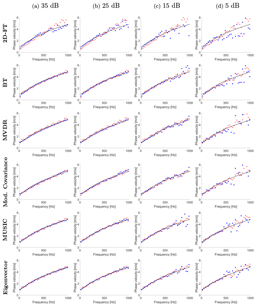
Phase velocity dispersion curves calculated for the numerical FDM tissue-mimicking viscoelastic models with assumed μ₁ = 1 kPa and μ₂ = 2 Pa·s. Results for six different methods are presented: 2D-FT, Blackman-Tukey (BT), MVDR, Modified Covariance, MUSIC, and Eigenvector. Results were calculated for the numerical viscoelastic phantoms with a SNR of (a) 35 dB, (b) 25 dB, (c) 15 dB, and (d) 5 dB. Blue dots and red stars represent results for a lateral distance of 0-25 mm and 0-6 mm, respectively. Continuous, black lines correspond to the analytical KV phase velocity curves.

Figure 4:

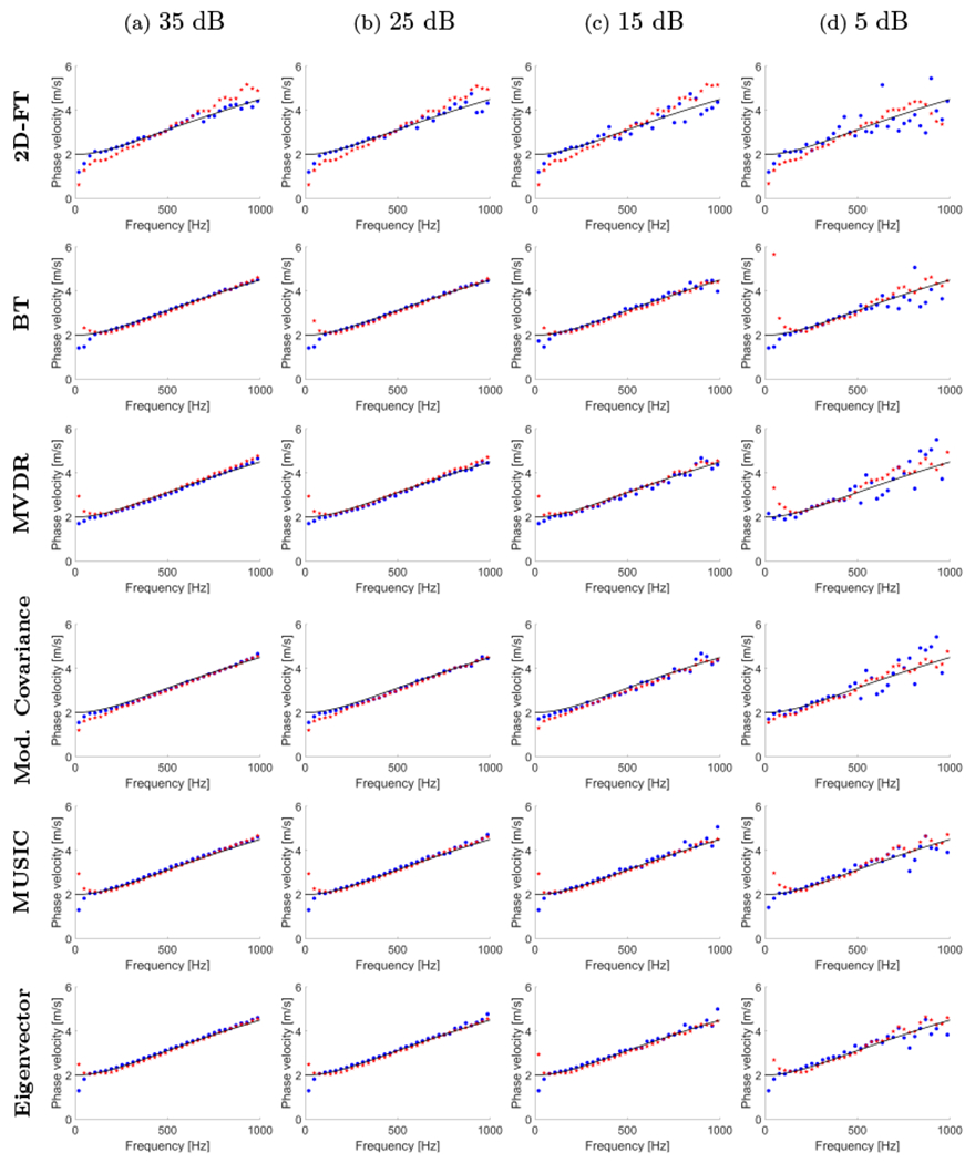
Phase velocity dispersion curves calculated for the numerical FDM tissue-mimicking viscoelastic models with assumed μ₁ = 4 kPa and μ₂ = 2 Pa·s. Results for six different methods are presented: 2D-FT, Blackman-Tukey (BT), MVDR, Modified Covariance, MUSIC, and Eigenvector. Results were calculated for the numerical viscoelastic phantoms with a SNR of (a) 35 dB, (b) 25 dB, (c) 15 dB, and (d) 5 dB. Blue dots and red stars represent results for a lateral distance of 0-25 mm and 0-6 mm, respectively. Continuous, black lines correspond to the analytical KV phase velocity curves.

Figure 5:

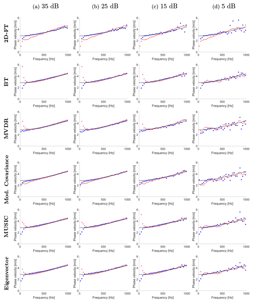
Phase velocity dispersion curves calculated for the numerical FDM tissue-mimicking viscoelastic models with assumed μ₁ = 8 kPa and μ₂ = 2 Pa·s. Results for six different methods are presented: 2D-FT, Blackman-Tukey (BT), MVDR, Modified Covariance, MUSIC, and Eigenvector. Results were calculated for the numerical viscoelastic phantoms with a SNR of (a) 35 dB, (b) 25 dB, (c) 15 dB, and (d) 5 dB. Blue dots and red stars represent results for a lateral distance of 0-25 mm and 0-6 mm, respectively. Continuous, black lines correspond to the analytical KV phase velocity curves.

Figure 6:

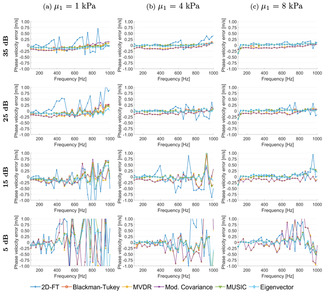
Phase velocity error calculated in a frequency range for shear wave particle velocity motion data measured in a lateral distance from 0-25 mm (blue dots in Figs. 3, 4, and 5). Results were estimated for the numerical tissue-mimicking viscoelastic models with assumed μ₁ of (a) 1 kPa, (b) 4 kPa, and (c) 8 kPa, with manually added white Gaussian noise, with a SNR of 35 dB, 25 dB, 15 dB, and 5 dB.

Figure 7:

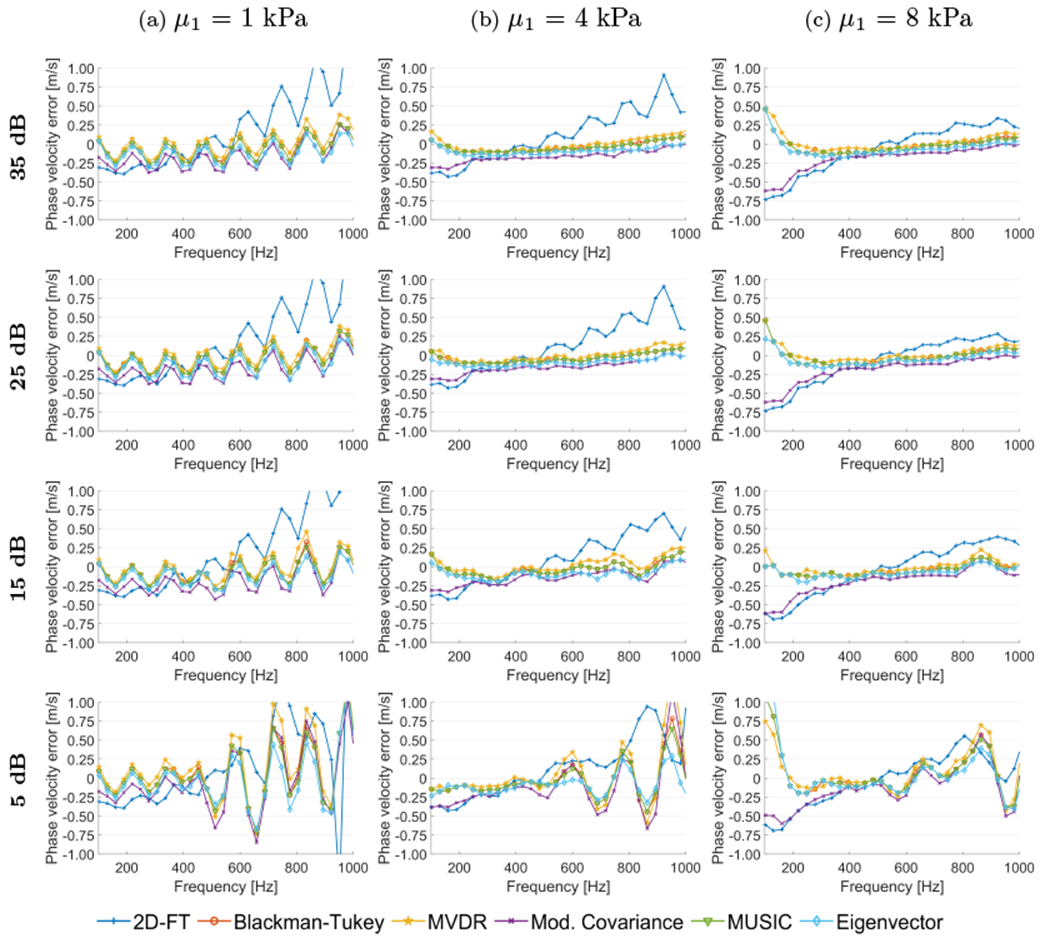
Phase velocity error calculated in a frequency range for shear wave particle velocity motion data measured in a lateral distance from 0-6 mm (red stars in Figs. 3, 4, and 5). Results were estimated for the numerical tissue-mimicking viscoelastic models with assumed μ₁ of (a) 1 kPa, (b) 4 kPa, and (c) 8 kPa, with manually added white Gaussian noise, with a SNR of 35 dB, 25 dB, 15 dB, and 5 dB.

Figures 6 and 7 show comparison of phase velocity errors calculated with respect to the reference dispersion curve (Eq. (14)) in the frequency domain. The error was calculated as a difference between computed phase velocity and a reference velocity (analytical dispersion curves). Errors in Figs. 6 and 7 refer to the results presented in Figs. 3, 4, and 5, respectively. Results for the 2D-FT method are most affected by the noise (Fig. 6). The MVDR and Modified Covariance approaches estimated the phase velocity within the investigated frequency range with lower error for all three numerical phantoms examined in this study, but the results are underestimated by about 0.1 m/s (Fig. 6). The MUSIC and Eigenvector techniques performed with the least error as can be seen in Fig. 6.

Figure 7 shows how performance of all the methods changes if a limited amount of spatial input data is truncated from 25 mm to 6 mm (x = 0-6 mm). A few differences can be clearly distinguished in comparison to the results for x = 0-25 mm shown in Fig. 6. First, oscillatory behavior can be seen for the softest (the most viscoelastic) phantom in Fig. 7a, for all the results. Second, for the models with μ₁ = 4 and 8 kPa higher deviation is present for lower frequencies which increases with higher material stiffness. The phase velocity error flattens as the frequency increases. Third, the error for 4 kPa and 8 kPa, for higher frequencies exhibits less variation than for the lateral segment length of 25 mm. This is clearly visible in Figs. 7b, and 7c for a SNR of 35, 25, and 15 dB. In addition, results for 2D-FT, for 6 mm are strongly deflected in comparison to Fig. 6 (x = 0-25 mm).

Boxplots of the phase velocity error within a range of 200-900 Hz, for the three numerical models investigated, were calculated for the data with a SNR of 35, 25, 15, and 5 dB, for 30 iterations each, respectively. Results are summarized in Fig. 8. The bottom and top edges of the box indicate the 25^th and 75^th percentiles, respectively. White circles represent the mean values of the phase velocity error, whereas a solid line within each box corresponds to a median value, calculated from 30 iterations and a frequency range from 200-900 Hz. Outliers were also plotted if values are greater than q₃+w(q₃−q₁) or less than q₁ − w(q₃ − q₁), where w is the maximum whisker length, and q₁ and q₃ are the 25^th and 75^th percentiles of the sample data, respectively. The parameter w was chosen to be 1.5. Interquartile range (IQR) quantitative evaluation can be made by calculation of a difference between 25^th and 75^th percentiles of the sample data as IQR = q₃ − q₁. Results for two different lateral segments are presented, 6 and 25 mm, respectively. Additionally, IQR values for each model and various SNR levels are summarized in Table 1.

Figure 8:

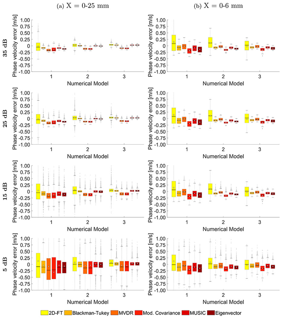
Boxplots computed for the phase velocity error calculated in a frequency range from 100-900 Hz, for shear wave particle velocity motion data measured in a lateral distance from (a) 0-25 mm, and (b) 0-6 mm. Phase velocity errors were calculated for the numerical FDM data, for 30 iterations with SNR value set to 35, 25, 15, and 5 dB, respectively.

Table 1:

IQR of the phase velocity error for 30 iterations and frequency range from 200 to 900 Hz. Results for six different methods and three numerical phantoms are summarized. Results are presented in the unit of [m/s].

μ1 [kPa]	METHOD	X = 0-25 mm				X = 0-6 mm
		SNR [dB]				SNR [dB]
		35	25	15	5	35	25	15	5
1	2D-FT	0.296	0.360	0.592	0.948	0.604	0.604	0.608	0.610
	BT	0.047	0.068	0.161	0.475	0.185	0.212	0.208	0.328
	MVDR	0.080	0.089	0.204	0.826	0.186	0.191	0.238	0.375
	Mod. Cov.	0.129	0.134	0.215	0.836	0.192	0.204	0.209	0.337
	MUSIC	0.043	0.069	0.163	0.498	0.204	0.204	0.213	0.327
	EV	0.043	0.055	0.140	0.428	0.210	0.212	0.205	0.309
4	2D-FT	0.101	0.153	0.288	0.536	0.390	0.431	0.410	0.415
	BT	0.034	0.039	0.071	0.209	0.070	0.075	0.068	0.169
	MVDR	0.058	0.053	0.110	0.476	0.080	0.083	0.078	0.202
	Mod. Cov.	0.053	0.056	0.111	0.493	0.059	0.059	0.075	0.183
	MUSIC	0.025	0.037	0.074	0.205	0.070	0.070	0.068	0.163
	EV	0.023	0.029	0.083	0.209	0.057	0.055	0.058	0.135
8	2D-FT	0.047	0.055	0.112	0.255	0.347	0.346	0.360	0.368
	BT	0.031	0.032	0.057	0.116	0.071	0.071	0.075	0.156
	MVDR	0.037	0.056	0.101	0.384	0.094	0.094	0.094	0.194
	Mod. Cov.	0.047	0.053	0.099	0.387	0.097	0.097	0.113	0.198
	MUSIC	0.027	0.029	0.056	0.114	0.072	0.071	0.077	0.162
	EV	0.030	0.028	0.055	0.119	0.091	0.097	0.091	0.141

For the numerical, viscoelastic models investigated the largest box plots are present for the 2D-FT method, from all the approaches examined in this work. The second non-parametric method, Blackman-Tukey, gives much improved results (smaller box plots) in relation to the 2D-FT. This behavior can be seen for all the models, SNR levels and two lateral segments. Considering a moderate noise level, e.g. 15 dB, and longer lateral distance (x = 0-25 mm), IQRs for μ₁ = 1 kPa (model 1) are 0.592 and 0.161 m/s for the 2D-FT and BT methods, respectively (Table 1). The parametric methods, MVDR and Modified Covariance, have higher IQR values than BT, at the level of 0.204 and 0.215 m/s, respectively. The high-resolution approaches on the other hand, MUSIC and Eigenvector, have IQRs equal to 0.163 and 0.140 m/s, respectively (Table 1). Considering the same phantom and SNR level but for shorter lateral segment length, i.e. 0-6 mm (Fig. 8b), increased IQRs are observed for most approaches. The non-parametric 2D-FT and BT methods have IQR of 0.608 and 0.208 m/s, and the parametric MVDR and Modified Covariance methods have 0.238 and 0.209 m/s, respectively. The high-resolution approaches exhibit slight increase of IQR to 0.213 and 0.205 m/s for the MUSIC and Eigenvector methods, respectively.

Less viscoelastic materials, with lower $\frac{{\mu }_2}{{\mu }_1}$ ratio, have lower variation (lower IQR) in calculated dispersion phase velocities, as can be seen in Fig. 8 and Table 1. For example, for viscoelastic model 3 (μ₁ = 8 kPa), SNR of 15 dB and the lateral segment length of 25 mm, IQR for 2D-FT is equal to 0.112 m/s. At the same time the BT results have an IQR of 0.057 m/s, which is at almost the same level as the IQR for the MUSIC and Eigenvector methods, i.e. 0.056 and 0.055 m/s, respectively. The parametric methods again exhibited higher IQRs than the BT and high-resolution approaches, 0. 101 and 0.099 m/s, respectively. Comparing these values with the IQRs for shorter lateral segment some differences can be observed out of which 2D-FT exhibited the largest IQR value change. In a similar way other phantoms and white Gaussian noise levels can be analyzed following Fig. 8 and Table 1.

4.2. Experimental TM Phantoms Results

In this section, the non-parametric, parametric and high-resolution methods were used for phase velocity dispersion curves calculation for the experimental TM phantom data. Three different custom made TM phantoms were investigated, and the results are shown in Figs. 9 and 10 for 25 mm and 6 mm lateral segment lengths, respectively. Two different acquisition positions were tested for each phantom.

Figure 9:

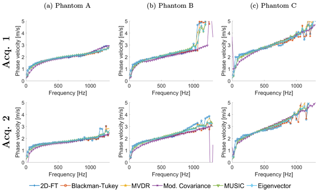
Phase velocity dispersion curves calculated for the custom-made tissue-mimicking viscoelastic phantoms for shear wave particle velocity motion data measured in a lateral distance from 0-25 mm. Results for six different methods are presented: 2D-FT, Blackman-Tukey (BT), MVDR, Modified Covariance, MUSIC, and Eigenvector. Results were calculated for two different acquisition positions for each phantom.

Figure 10:

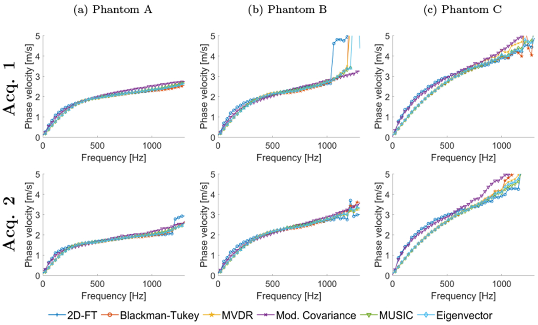
Phase velocity dispersion curves calculated for the custom-made tissue-mimicking viscoelastic phantoms for shear wave particle velocity motion data measured in a lateral distance from 0-6 mm. Results for six different methods are presented: 2D-FT, Blackman-Tukey (BT), MVDR, Modified Covariance, MUSIC, and Eigenvector. Results were calculated for two different acquisition positions for each phantom.

Generally, all the approaches examined in this paper estimated dispersion curves with similar trends, within all the experimental phantoms, for the lateral segment length of 25 mm (Fig. 9). The biggest differences between the methods are observed for frequencies below 250 Hz and above 1000 Hz. The Modified Covariance method estimated dispersion curves slightly lower in comparison to other approaches for frequencies below 250 Hz. For frequencies above 1000 Hz, the 2D-FT had higher variations for Phantom A and acquisition 2 compared to other techniques (Fig. 9a). For Phantoms B and C all the approaches show variations for higher frequencies in Figs. 9b and 9c. The smallest ones are observed for the Modified Covariance method for all the phantoms and acquisitions examined. The MUSIC and Eigenvector methods performed with lower variation compared to the 2D-FT, BT and MVDR techniques.

Some differences between the methods are also observed for the short lateral segment length shown in Fig. 10. All the methods performed similarly for Phantom A. The Modified Covariance gives the lowest variation above 1000 Hz for Phantom B. Stiffer Phantom C shows higher deviations between the methods. Dispersion curves for the 2D-FT and Modified Covariance are separated from phase velocities calculated using other approaches.

5. Discussion

Dispersion curves, represented in wavenumber-frequency or velocity-frequency domains, play an important role when analyzing material properties of biological tissues. The most common method for dispersion relation estimation is based on the fast Fourier transform (2D-FT). For many applications, FFT-based methods produce sufficiently good results. However, more advanced methods can offer better frequency resolution, and less variance (Hayes (1996); Williams and Madisetti (1997); Trefethen (2000); Vaseghi (2008)).

In this work, we present a comparison between the selected non-parametric, parametric and high-resolution methods used for shear wave dispersion curves calculation of viscoelastic materials. The methods’ robustness was examined on simulated data from FDM models of shear wave propagation induced by acoustic radiation force in viscoelastic media. FDM models do not take into account displacement underestimation bias which occurs during ultrasound motion detection, which is a limitation here. As a result, only adding Gaussian noise to the resulting particle velocity from the numerical models may not completely capture the noise model experienced in practice. We compared the performance of various methods using different levels of added white Gaussian noise as shown in Figs. 3–5 and more thoroughly with an analysis of the error in Figs. 6 and 7, and box plots in Fig. 8, and Table 1, respectively. The results showed that the Blackman-Tukey method and high-resolution approaches give the lowest phase velocity variation. We observed the qualitative similarities between the simulation and experimental data. Moreover, in this study, we have experimental data in viscoelastic phantoms to supplement the simulation data.

The methods were also tested with experimental data in custom made TM viscoelastic phantoms. The results were generally similar between the examined methods. We also examined the performance of all the methods for the limited shear wave motion particle velocity data (short lateral segment length).

It should be mentioned that the wave velocity dispersion results from all the approaches are dependent on the data input to the algorithm. It was observed in previous works that adjusting the distance range of the data, i.e., the distance from the source can cause changes to the dispersion (Rouze et al. (2017); Kijanka et al. (2018, 2019)). Shear waves at higher frequencies typically undergo higher attenuation and therefore do not propagate as far leading to shorter lateral imaging lengths (Kijanka and Urban (2020a)). In this study, we chose the distance from the source to be 0 mm since shear wave motion data measured at a very close spatial distance includes information about higher frequencies. Hence, we were able to estimate phase velocity dispersion curves up to 1000 Hz, even for highly viscoelastic (high $\frac{{\mu }_2}{{\mu }_1}$ ratio) tissue-mimicking numerical phantom shown in Fig. 3. The goal of this work was to examine different methods performance for the same shear wave input data, and the measured lateral segment length was the same for all the approaches.

An important issue in the selection of dispersion curves estimation technique is the performance of the estimator. In this paper, it was shown that, in comparing one method to another, there is a different level of phase velocity variation within a frequency range. The non-parametric methods are not designed to incorporate information that may be available about the process into the estimation processing. In some applications this may be a limitation. Generally, parametric methods produce smoother estimates of the power spectrum than non-parametric methods, however they are subject to higher error from model misspecification. The Blackman-Tukey method, which makes no assumptions about the process, produces more accurate estimates of the dispersion curves than the parametric techniques, as was shown in Figs. 3–8.

The high-resolution methods assume that measured signals are a sum of complex exponentials or sinusoids in white noise. They tend to estimate the frequencies of the complex exponentials. These methods do not yield true power spectral density estimates. They do not preserve process power between the time and frequency domains, and the original signal cannot be recovered by taking the inverse Fourier transform of the frequency estimate. Whereby, the wavenumber-frequency distribution computed using MUSIC or EV cannot be used to the shear wave attenuation estimation using, e.g. the attenuation measuring ultrasound shear elastography (AMUSE) method (Nenadic et al. (2016)).

We can conclude from our study that more advanced approaches, like MUSIC or Eigenvector, are more difficult to implement and they have input parameters that should be known a priori (number of exponentials that exist within the measured signal). For some scenarios there is no need to apply MUSIC or other advanced techniques but the non-parametric Blackman-Tukey approach may be sufficiently used, like for example for materials with higher $\frac{{\mu }_2}{{\mu }_1}$ ratio and high SNR. Additionally, for MUSIC and the Eigenvector we need to provide two input parameters (number of signals to be found and size of the covariance matrix) whereas, for Blackman-Tukey the length of the smoothing window is provided. The BT approach does not require any a priori knowledge about the measured process.

It is worth noting that in our work we investigated tissue-mimicking viscoelastic bulk media, where a single propagating shear wave was generated and measured. Hence, only one dispersion curve was estimated for each dataset using the methods examined. All the parameters for all the methods discussed in our manuscript were evaluated for these kinds of bulk materials. These methods could be used to estimate dispersion curves in other applications where multiple modes are present such as for guided waves in arteries or materials with finite thickness. In those cases, other parameter values may provide better results. This however, would have to be investigated separately, and is beyond the scope of this work.

6. Conclusions

We tested six different approaches to spectrum estimation used for dispersion curves calculation in viscoelastic materials, including the most known and widely used 2D-FT, and we performed a robustness study of these techniques. The high-resolution methods give the lowest phase velocity variation. Nevertheless, the Blackman-Tukey approach exhibits similar performance and can be interchangeably used for shear wave phase velocity dispersion curves calculation. Although, each method differs in its resolution and variance, the general performance is fundamentally limited by the amount of data that is available. Future work will be devoted to develop methods that improve robustness of spectrum estimation approaches for higher frequencies, i.e. above 1000 Hz, for the phantoms tested in this work.

Appendix

To support our selection of the input parameters used for specific methods investigated in this work, we conducted a parametric study in Fig. 11. Figure 11 shows parametric studies of the (a) Blackman-Tukey, (b) MVDR, (c) Modified Covariance, (d) MUSIC, and (e) Eigenvector methods, respectively. Phase velocity errors were calculated for various controlling parameters, for five selected values, of each method to test their influence on the tested data. The numerical FDM tissue-mimicking viscoelastic model with μ₁ = 4 kPa and μ₂ = 2 Pa·s, and a SNR of 15 dB, as an example, was used for these investigations. Results in Fig. 11 give an idea about the performance of the methods if other values of the parameters were used for the dispersion curve estimation in the viscoelastic bulk materials.

Figure 11:

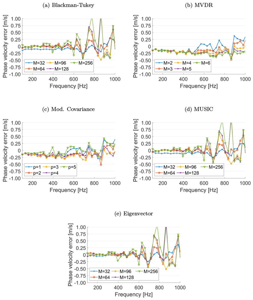
Parametric studies of the (a) Blackman-Tukey, (b) MVDR, (c) Modified Covariance, (d) MUSIC, and (e) Eigenvector methods, respectively. Phase velocity errors were calculated for various controlling parameters of each method to test their influence on the data. The numerical FDM tissue-mimicking viscoelastic model with μ₁ = 4 kPa and μ₂ = 2 Pa·s, and a SNR of 15 dB was used for these investigations. Shear wave particle velocity motion data measured in a lateral distance from 0-25 mm were utilized.

References

- Alleyne D, Cawley P, 1991. A two-dimensional fourier transform method for the measurement of propagating multimode signals. The Journal of the Acoustical Society of America 89, 1159–1168. [Google Scholar]
- Amador C, Urban M, Kinnick R, Chen S, Greenleaf JF, 2013. In vivo swine kidney viscoelasticity during acute gradual decrease in renal blood flow: pilot study. Revista Ingeniería Biomédica 7, 68–78. [PMC free article] [PubMed] [Google Scholar]
- Amador C, Urban MW, Chen S, Greenleaf JF, 2011. Shearwave dispersion ultrasound vibrometry (SDUV) on swine kidney. IEEE Trans. Ultrason., Ferroelect., Freq. Control 58. [DOI] [PMC free article] [PubMed] [Google Scholar]
- Bartlett M, 1948. Smoothing periodograms from time-series with continuous spectra. Nature 161, 686–687. [Google Scholar]
- Bercoff J, Tanter M, Muller M, Fink M, 2004. The role of viscosity in the impulse diffraction field of elastic waves induced by the acoustic radiation force. IEEE Transactions on Ultrasonics, Ferroelectrics, and Frequency Control 51, 1523–1536. [DOI] [PubMed] [Google Scholar]
- Bernal M, Nenadic I, Urban MW, Greenleaf JF, 2011. Material property estimation for tubes and arteries using ultrasound radiation force and analysis of propagating modes. The Journal of the Acoustical Society of America 129, 1344–1354. [DOI] [PMC free article] [PubMed] [Google Scholar]
- Blackman RB, Tukey JW, 1958. The measurement of power spectra from the point of view of communications engineering - Part I. Bell System Technical Journal 37, 185–282. [Google Scholar]
- Capon J, 1969. High-resolution frequency-wavenumber spectrum analysis. Proceedings of the IEEE 57, 1408–1418. [Google Scholar]
- Catheline S, Gennisson JL, Delon G, Fink M, Sinkus R, Abouelkaram S, Culioli J, 2004. Measurement of viscoelastic properties of homogeneous soft solid using transient elastography: an inverse problem approach. The Journal of the Acoustical Society of America 116, 3734–3741. [DOI] [PubMed] [Google Scholar]
- Chen D, McGough RJ, 2008. A 2d fast near-field method for calculating near-field pressures generated by apodized rectangular pistons. The Journal of the Acoustical Society of America 124, 1526–1537. [DOI] [PMC free article] [PubMed] [Google Scholar]
- Chen S, Fatemi M, Greenleaf JF, 2004. Quantifying elasticity and viscosity from measurement of shear wave speed dispersion. The Journal of the Acoust. Soc. of America 115, 2781–2785. [DOI] [PubMed] [Google Scholar]
- Chen S, Sanchez W, Callstrom MR, Gorman B, Lewis JT, Sanderson SO, Greenleaf JF, Xie H, Shi Y, Pashley M, Shamdasani V, Lachman M, Metz S, 2013. Assessment of liver viscoelasticity by using shear waves induced by ultrasound radiation force. Radiology 266, 964–970. [DOI] [PMC free article] [PubMed] [Google Scholar]
- Chen S, Urban MW, Pislaru C, Kinnick R, Zheng Y, Yao A, Greenleaf JF, 2009. Shearwave dispersion ultrasound vibrometry (SDUV) for measuring tissue elasticity and viscosity. IEEE Trans. Ultrason., Ferroelect., Freq. Control 56, 55–62. [DOI] [PMC free article] [PubMed] [Google Scholar]
- Couade M, Pernot M, Prada C, Messas E, Emmerich J, Bruneval P, Criton A, Fink M, Tanter M, 2010. Quantitative assessment of arterial wall biomechanical properties using shear wave imaging. Ultrasound in medicine & biology 36, 1662–1676. [DOI] [PubMed] [Google Scholar]
- Deffieux T, Gennisson JL, Bousquet L, Corouge M, Cosconea S, Amroun D, Tripon S, Terris B, Mallet V, Sogni P, et al. , 2015. Investigating liver stiffness and viscosity for fibrosis, steatosis and activity staging using shear wave elastography. Journal of hepatology 62, 317–324. [DOI] [PubMed] [Google Scholar]
- Deffieux T, Montaldo G, Tanter M, Fink M, 2009. Shear wave spectroscopy for in vivo quantification of human soft tissues visco-elasticity. IEEE Trans. Med. Imag 28, 313–322. [DOI] [PubMed] [Google Scholar]
- FOCUS, 2019. Fast Object-Oriented C++ Ultrasound Simulator. https://www.egr.msu.edu/~fultras-web/.
- Gennisson JL, Deffieux T, Macé E, Montaldo G, Fink M, Tanter M, 2010. Viscoelastic and anisotropic mechanical properties of in vivo muscle tissue assessed by supersonic shear imaging. Ultrasound in medicine & biology 36, 789–801. [DOI] [PubMed] [Google Scholar]
- Hayes MH, 1996. Statistical digital signal processing and modeling. John Wiley & Sons. [Google Scholar]
- Haykin S, Kesler S, 1979. Prediction-error filtering and maximum-entropy spectral estimation, in: Nonlinear methods of spectral analysis. Springer, pp. 9–72. [Google Scholar]
- Johnson D, DeGraaf S, 1982. Improving the resolution of bearing in passive sonar arrays by eigenvalue analysis. IEEE Transactions on Acoustics, Speech, and Signal Processing 30, 638–647. [Google Scholar]
- Kasai C, Namekawa K, Koyano A, Omoto R, 1985. Real-time two-dimensional blood flow imaging using an autocorrelation technique. IEEE Trans. Sonics Ultrason 32, 458–464. [Google Scholar]
- Kay S, Marple S, 1979. Sources of and remedies of spectral line-splitting in ar spectrum analysis, in: Proc. IEEE Int. Conf. ASSP, pp. 151–154. [Google Scholar]
- Kay SM, 1993. Fundamentals of statistical signal processing. Prentice Hall PTR. [Google Scholar]
- Kijanka P, Ambrozinski L, Urban MW, 2019. Two point method for robust shear wave phase velocity dispersion estimation of viscoelastic materials. Ultrasound in Medicine & Biology 45, 2540–2553. [DOI] [PMC free article] [PubMed] [Google Scholar]
- Kijanka P, Qiang B, Song P, Amador C, Chen S, Urban MW, 2018. Robust phase velocity dispersion estimation of viscoelastic materials used for medical applications based on the multiple signal classification method. IEEE Trans. Ultrason., Ferroelect., Freq. Control 65, 423–439. [DOI] [PMC free article] [PubMed] [Google Scholar]
- Kijanka P, Urban MW, 2020a. Local phase velocity based imaging (LPVI) of viscoelastic phantoms and tissues. IEEE Trans. Ultrason., Ferroelect., Freq. Control doi:doi: 10.1109/TUFFC.2020.2968147. [DOI] [PMC free article] [PubMed] [Google Scholar]
- Kijanka P, Urban MW, 2020b. Two-Point Frequency Shift Method for Shear Wave Attenuation Measurement. IEEE Transactions on Ultrasonics, Ferroelectrics, and Frequency Control 67, 483–496. [DOI] [PMC free article] [PubMed] [Google Scholar]
- Kumar V, Denis M, Gregory A, Bayat M, Mehrmohammadi M, Fazzio R, Fatemi M, Alizad A, 2018. Viscoelastic parameters as discriminators of breast masses: Initial human study results. PloS one 13. [DOI] [PMC free article] [PubMed] [Google Scholar]
- Montaldo G, Tanter M, Bercoff J, Benech N, Fink M, 2009. Coherent plane-wave compounding for very high frame rate ultrasonography and transient elastography. IEEE Trans. Ultrason., Ferroelect., Freq. Control 56, 489–506. [DOI] [PubMed] [Google Scholar]
- Muller M, Gennisson JL, Deffieux T, Tanter M, Fink M, 2009. Quantitative viscoelasticity mapping of human liver using supersonic shear imaging: preliminary in vivo feasability study. Ultrasound in medicine & biology 35, 219–229. [DOI] [PubMed] [Google Scholar]
- Nenadic IZ, Qiang B, Urban MW, Zhao H, Sanchez W, Greenleaf JF, Chen S, 2016. Attenuation measuring ultrasound shearwave elastography and in vivo application in post-transplant liver patients. Physics in medicine and biology 62, 484. [DOI] [PMC free article] [PubMed] [Google Scholar]
- Nguyen MM, Zhou S, Robert J.l., Shamdasani V, Xie H, 2014. Development of oil-in-gelatin phantoms for viscoelasticity measurement in ultrasound shear wave elastography. Ultrasound in medicine & biology 40, 168–176. [DOI] [PubMed] [Google Scholar]
- Nightingale K, McAleavey S, Trahey G, 2003. Shear-wave generation using acoustic radiation force: in vivo and ex vivo results. Ultrasound in medicine & biology 29, 1715–1723. [DOI] [PubMed] [Google Scholar]
- Nightingale KR, Palmeri ML, Nightingale RW, Trahey GE, 2001. On the feasibility of remote palpation using acoustic radiation force. The Journal of the Acoustical Society of America 110, 625–634. [DOI] [PubMed] [Google Scholar]
- Nightingale KR, Rouze NC, Rosenzweig SJ, Wang MH, Abdelmalek MF, Guy CD, Palmeri ML, 2015. Derivation and analysis of viscoelastic properties in human liver: Impact of frequency on fibrosis and steatosis staging. IEEE Trans. Ultrason., Ferroelect., Freq. Control 62, 165–175. [DOI] [PMC free article] [PubMed] [Google Scholar]
- Nuttall AH, 1976. Spectral analysis of a univariate process with bad data points, via maximum entropy and linear predictive techniques. Technical Report. NAVAL UNDERWATER SYSTEMS CENTER; NEWPORTRI. [Google Scholar]
- Pisarenko VF, 1973. The retrieval of harmonics from a covariance function. Geophysical Journal International 33, 347–366. [Google Scholar]
- Ribeiro PF, Duque CA, Ribeiro PM, Cerqueira AS, 2013. Power systems signal processing for smart grids. John Wiley & Sons. [Google Scholar]
- Rouze NC, Deng Y, Palmeri ML, Nightingale KR, 2017. Accounting for the spatial observation window in the 2-d fourier transform analysis of shear wave attenuation. Ultrasound in Medicine & Biology 43, 2500–2506. [DOI] [PMC free article] [PubMed] [Google Scholar]
- Rouze NC, Palmeri ML, Nightingale KR, 2015. An analytic, fourier domain description of shear wave propagation in a viscoelastic medium using asymmetric gaussian sources. The Journal of the Acoustical Society of America 138, 1012–1022. [DOI] [PMC free article] [PubMed] [Google Scholar]
- Sarvazyan A, Hall T, Urban M, Fatemi M, Aglyamov S, Garra B, 2011. Elasticity imaging-an emerging branch of medical imaging. an overview. Curr. Med. Imaging Rev 7, 255–282. [DOI] [PMC free article] [PubMed] [Google Scholar]
- Schmidt R, 1986. Multiple emitter location and signal parameter estimation. IEEE transactions on antennas and propagation 34, 276–280. [Google Scholar]
- Shon S, Mehrotra K, 1984. Performance comparison of autoregressive estimation methods, in: ICASSP’84. IEEE International Conference on Acoustics, Speech, and Signal Processing, IEEE; pp. 581–584. [Google Scholar]
- Song P, Macdonald MC, Behler RH, Lanning JD, Wang MH, Urban MW, Manduca A, Zhao H, Callstrom MR, Alizad A, et al. , 2015. Two-dimensional shear-wave elastography on conventional ultrasound scanners with time-aligned sequential tracking (tast) and shear elastography (cuse). IEEE Trans. Ultrason., Ferroelect., Freq. Control 62, 290–302. [DOI] [PMC free article] [PubMed] [Google Scholar]
- Tanter M, Bercoff J, Athanasiou A, Deffieux T, Gennisson JL, Montaldo G, Muller M, Tardivon A, Fink M, 2008. Quantitative assessment of breast lesion viscoelasticity: initial clinical results using supersonic shear imaging. Ultrasound in medicine & biology 34, 1373–1386. [DOI] [PubMed] [Google Scholar]
- Thomson DJ, 1982. Spectrum estimation and harmonic analysis. Proceedings of the IEEE 70, 1055–1096. [Google Scholar]
- Trefethen LN, 2000. Spectral methods in MATLAB. Siam. [Google Scholar]
- Ulrych TJ, Clayton RW, 1976. Time series modelling and maximum entropy. Physics of the Earth and Planetary Interiors 12, 188–200. [Google Scholar]
- Vaseghi SV, 2008. Advanced digital signal processing and noise reduction. John Wiley & Sons. [Google Scholar]
- Virieux J, 1986. P-SV wave propagation in heterogeneous media: Velocity-stress finite-difference method. Geophysics 51, 889–901. [Google Scholar]
- Welch P, 1967. The use of fast fourier transform for the estimation of power spectra: a method based on time averaging over short, modified periodograms. IEEE Transactions on audio and electroacoustics 15, 70–73. [Google Scholar]
- Williams DB, Madisetti V, 1997. Digital signal processing Handbook. CRC Press, Inc. [Google Scholar]
- Zeng X, McGough RJ, 2008. Evaluation of the angular spectrum approach for simulations of near-field pressures. The Journal of the Acoustical Society of America 123, 68–76. [DOI] [PMC free article] [PubMed] [Google Scholar]