Automatic quality assessment for 2D fetal sonographic standard plane based on multitask learning

Abstract

The quality control of fetal sonographic (FS) images is essential for the correct biometric measurements and fetal anomaly diagnosis. However, quality control requires professional sonographers to perform and is often labor-intensive. To solve this problem, we propose an automatic image quality assessment scheme based on multitask learning to assist in FS image quality control. An essential criterion for FS image quality control is that all the essential anatomical structures in the section should appear full and remarkable with a clear boundary. Therefore, our scheme aims to identify those essential anatomical structures to judge whether an FS image is the standard image, which is achieved by 3 convolutional neural networks. The Feature Extraction Network aims to extract deep level features of FS images. Based on the extracted features, the Class Prediction Network determines whether the structure meets the standard and Region Proposal Network identifies its position. The scheme has been applied to 3 types of fetal sections, which are the head, abdominal, and heart. The experimental results show that our method can make a quality assessment of an FS image within less a second. Also, our method achieves competitive performance in both the segmentation and diagnosis compared with state-of-the-art methods.

1. Introduction

1.1. Background

Fetal sonographic (FS) examinations are widely applied in clinical settings due to its noninvasive nature, reduced cost, and real-time acquisition.^[1] FS examinations are consisted of first, second, and third trimester examinations, and limited examination,^[2] which covers a range of critical inspections such as evaluation of a suspected ectopic pregnancy,^[3,4] and confirmation of the presence of an intrauterine pregnancy.^[5–7] The screening and evaluation of fetal anatomy are critical during the second and third trimester examinations. The screening is usually assessed by ultrasound after approximately 18 weeks’ gestational (menstrual) age. According to a survey,^[8] neonatal mortality in the United States in 2016 was 5.9 deaths per 1000 live births, and birth defects are the leading cause of infant deaths, accounting for 20% of all infant deaths. Besides, congenital disabilities occur in 1 in every 33 babies (about 3% of all babies) born in the United States each year. In this case, the screening and evaluation of fetal anomaly will provide crucial information to families prior to the anticipated birth of their child on diagnosis, underlying etiology, and potential treatment options, which can greatly improve the survival rate of the fetus. However, the physiological evaluation of fetal anomaly requires well-trained and experienced sonographers to obtain standard planes. Although a detailed quality control guideline was developed for the evaluation of standard plan,^[8] the accuracy of the measurements is highly dependent on the operator's training skill and experience. According to a study,^[8] intraobserver and interobserver variability exist in routine practice, and inconsistent image quality can lead to variances in specific anatomic structures captured by different operators. Furthermore, in areas where medical conditions are lagging, there is a lack of well-trained doctors, which makes FS examinations impossible to perform. To this end, automatic approaches for FS image quality assessment are needed to ensure that the image is captured as required by guidelines and provide accurate and reproducible fetal biometric measurements.^[9]

To obtain standard planes and assess the quality of FS images, it is necessary that all the essential anatomical structures in the imaging should appear full and remarkable with clear boundary.^[2] For each medical section, there are different essential structures. In our research, we consider 3 medical sections: the heart section, the head section, and the abdominal section. The essential structures corresponding to these sections are given in Table 1. The list of essential anatomical structures used to evaluate the image quality is defined by the guideline^[2] and further refined by 2 senior radiologists with more than 10 years of experience of FS examination at the West China Second Hospital Sichuan University, Chengdu, China. A comparison of standard and nonstandard planes can be illustrated in Figure 1.

Table 1.

Essential anatomical structures for different sections.

Section name	Essential anatomical structure
Head	Cavum septi pellucidi
	Thalamus
	Third ventricle
	Brain midline
	Lateral sulcus
	Choroid plexus
Abdominal	Spine
	Umbilical vein
	Aorta
	Stomach
Heart	Umbilical vein
	Umbilical vein
	Right ventricle
	Right atrium
	Descending aorta

Figure 1.

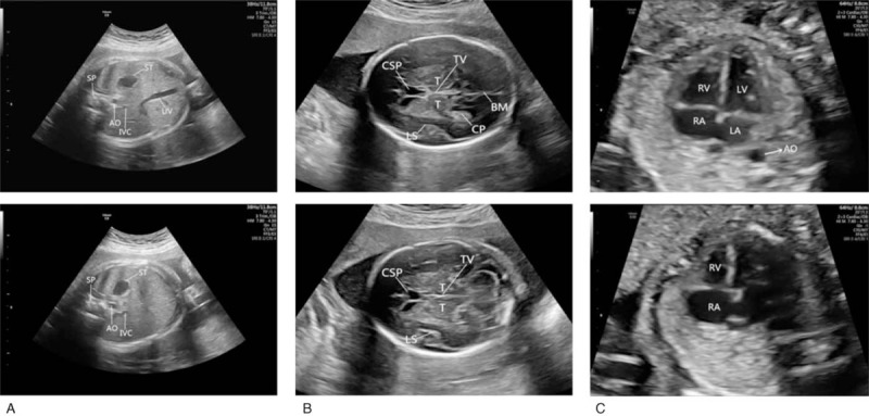
Comparison of the standard plane (upper row) and nonstandard plane (lower row) in 3 sections. A, The lower abdominal FS image does not show the umbilical vein. B, The lower head FS image does not show the brain midline and the choroid plexus. C, The lower heart FS image does not show the left ventricle, left atrium, and descending aorta.

There are various types of challenges concerning the automatic quality control of FS images. As illustrated in Figure 2, the main challenges can be divided into 3 types: the first type is that the image usually suffers from the influence of noise and shadowing effect, the second type is that similar anatomical structures could be confused due to the low resolution of the images, and the third type is that the fetal location during the scanning is unstable which will cause the rotation of some anatomical structure. The first type of challenges can only be solved by using more advanced scanning machines, but we can tackle the rest 2 challenges by a more scientific approach. Specifically, the purpose of our research can be summarized as follows:

Figure 2.

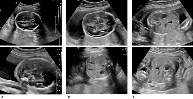
Illustration of different types of challenges. A, The white arrows show the substantial interference of noise and shadowing effect. B, In the upper graph, the blue box represents the real brain midline, and the orange box is the confusing anatomical structure with a similar shape. In the lower figure, the orange box represents the actual gallbladder, and the blue box represents the real umbilical vein. These 2 structures have a very similar shape. C, FS images with different fetal positions, which will cause significant variations for the appearance of the images. FS = fetal sonographic.

• Propose an automatic fetal sonographic image quality control framework for the segmentation and classification of the 2-dimensional fetal heart standard plane, which is highly robust against the interference of image rotation and similar structures, and the segmentation speed is quite fast to meet the clinical requirements fully.

• Improve the accuracy of the detection and classification further compared with state-of-the-art methods by using many recent advanced object detection technologies.

• Generalize the framework so that it can be well applied to other standard planes.

1.2. Related work

In recent years, deep learning techniques have been widely applied in many medical imaging fields due to the technique's stability and efficiency, such as anatomical object detection and segmentation ^[10–12] and brain abnormalities segmentation.^[13,14] Accordingly, many intelligent automatic diagnostic techniques for FS images have been proposed. For example, Deepika et al^[15] proposed a novel framework to diagnose the fetal anomaly by using ultrasound images. In the framework, it adopts U-Net architecture with Hough transformation to segment the abdominal region, and then a multistage convolutional neural network (CNN) is designed to extract the hidden features of FS images. The experiment shows it outperforms other CNN-based approach.^[15] Lin et al^[16] proposed a multitask CNN framework to address the problem of standard plane detection and quality assessment of fetal head ultrasound images. Under the framework, they introduced prior clinical and statistical knowledge to reduce the false detection rate further. The detection speed of this method is quite fast, and the result achieves promising performance compared with state-of-the-art methods.^[16] Xu et al^[17] proposed an integrated learning framework based on deep learning to perform view diagnosis and landmark detection of the structures in the fetal abdominal ultrasound image simultaneously. The automatic framework achieved a higher diagnosis accuracy better than clinical experts, and it also reduced landmark-based measurement errors.^[17] Wu et al proposed a computerized FS image quality assessment scheme to assist the quality control in the clinical obstetric examination of the fetal abdominal region. This method utilizes the local phase features along with the original fetal abdominal ultrasound images as input to the neural network. The proposed scheme achieved competitive performance in both view diagnosis and region localization.^[18] Chang et al^[19] proposed an automatic mid-sagittal plane (MSP) assessment method for categorizing the 3D fetal ultrasound images. This scheme also analyzes corresponding relationships between resulting MSP assessments and several factors, including image qualities and fetus conditions. It achieves a correct high rate for the results of MSP detection. Kumar and Sriram et al proposed an automatic method for fetal abdomen scan-plane identification based on 3 critical anatomical landmarks: the spine, stomach, and vein. In their approach, a Biometry Suitability Index (BSI) is proposed to judge whether the scan plane can be used for biometry based on detected anatomical landmarks. The results of the proposed method over video sequences were closely similar to the clinical expert's assessment of scan-plane quality for biometry.^[20] Baumgartner et al^[21] proposed a novel framework based on convolutional neural networks to automatically detect 13 standard fetal views in freehand 2D ultrasound data and provide localization of the anatomical structures through a bounding box. A notable innovation is that the network learns to localize the target anatomy using weak supervision based on image-level labels only.^[21] Namburete et al^[22] proposed a multitask, fully convolutional neural network framework to address the problem of 3D fetal brain localization, alignment to a referential coordinate system, and structural segmentation. This method optimizes the network by learning features shared within the input data belonging to the correlated tasks, and it achieves a high brain overlap rate and low eye localization error.^[22] However, there are no existing automatic quality control methods for fetal heart planes, and the detection accuracy of existing methods on other planes is relatively low due to the use of the outdated design of neural networks. Therefore, it is desirable to propose a more efficient framework that can not only provide accurate clinical assessment in fetal heart plane but can also increase the segmentation accuracy in other planes.

2. Methods

The framework of our methods can be illustrated in Figure 3. First, the original image is smoothed by the Gaussian filter, and input to feature extraction network (FEN). Second, FEN will extract a deep level feature of image by convolutional neural network and input to Region Proposal Network (RPN) and Class Prediction Network (CPN) respectively. Then CPN will judge whether the organs meet the standard as well as predict the class, and RPN will locate the position of essential organs with the help of feature pyramid network. Lastly, the 2 networks will combine information together and output the final result. In this section, we will briefly introduce the network structure and then elaborate the feature extraction, the region of interest (ROI) localization, and the organ diagnosis in detail. Our study is approved by Ethics Committee of West China Second Hospital Sichuan University.

Figure 3.

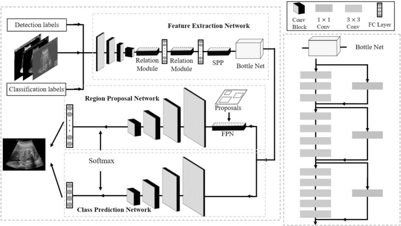
The framework of our method. We train the network end-to-end to ensure the best performance. The framework contains 3 sections: Feature Extraction Network (FEN), Region Proposal Network (RPN), and Class Prediction Network (CPN). The will help to extract the deep-level features of the image with the help of the relation module and Spatial Pyramid Pooling (SPP) layer, which is the input to RPN and CPN. The RPN will locate the position of essential structures based on the anchors generated by Feature Pyramid Network (FPN), and the CPN will help to judge and classify the structures. The final output will be a quality assessment of each essential structure and its location.

2.1. Feature extraction network

In the feature extraction network, we have made many improvements compared with the traditional CNN-based approaches: the convolutional neural network is used as a thematic framework, and many state-of-the-art deep learning techniques such as relation module, spatial pyramid pooling (SPP) layer, are integrated into the framework to further increase the feature extraction efficiency. The CNN has unique advantages in speech recognition and image processing with its special structure of local weight sharing, which can greatly reduce the number of parameters and improve the accuracy of recognition.^[23–25] CNN typically consists of pairs of convolutional layers and average pooling layers and fully connected (FC) layers. In convolutional layer, several output feature maps can be obtained by the convolutional calculation between input layer and kernel. Specifically, suppose $f_m^n$ denotes the mth output feature map in layer n, $f_k^{n-1}$ denotes the kth feature map in n – 1 layer, $W_m^n$ denotes the kernel generating that feature map, then we can get:

$$f_m^n=\text{relu}(\sum _{k=1}^N(W_m^n*f_k^{n-1})+b^n)$$

where $b^n$ is the bias term in the nth layer, relu denotes rectified linear unit, and is defined as: relu(x)=max(x,0). It is also worth mentioning that we use global average pooling (GAP) instead of local pooling for pooling layers. The aim is to use GAP to replace FC layer, which can regularize the structure of the entire network to prevent overfitting.^[26] The setting of convolution layer is shown in Table 2.

Table 2.

The setting of convolutional layer.

Layer	Kernel size	Channel depth	Stride
C1	3	128	2
C2	3	256	2
C3	3	512	2
C4	3	1024	2
C5	3	2048	2

To fully utilize relevant features between objects and further improve segmentation accuracy, we introduce the relation module presented by Hu.^[27] Specifically, first the geometry weight is defined as:

$$w_G^{mn}=\max \{0,W_G\cdot {\epsilon }_G(f_G^m,f_G^n)\}$$

where $f_G^m$ and $f_G^n$ are geometric features, ${\epsilon }_G$ is a dimensional lifting transformation by using concatenation. After that, the appearance weight is defined as:$w_A^{mn}=\frac{dot(W_K{f}_A^m,W_Q{f}_A^n)}{\sqrt{d_k}}$

where $W_K$ and $W_Q$ are the pixel weights from the previous network. Then the relation weight indicating the impact from other objects is computed as:

$$w^{mn}=\frac{w_G^{mn}\cdot \exp (w_A^{mn})}{\sum _k{w}_G^{kn}\cdot \exp (w_A^{kn})}$$

Lastly, the relation feature of the whole object set with respect to the $n^{th}$ object is defined as

$$f_R(n)=\sum _m{w}^{mn}\cdot (W_V\cdot f_A^m)$$

This module achieves a great performance in the instance recognition and duplicate removal, which increases the segmentation accuracy significantly.

The SPP layer we use here denotes the SPP layer presented by He et al.^[28] Specifically, the response map after FC layer is divided into 1 × 1 (pyramid base), 2 × 2 (lower middle of the pyramid), 4 × 4 (higher middle of the pyramid), 16 × 16 (pyramid top) 4 submaps and do max pooling separately. A problem with the traditional CNN network for feature extraction is that there is a strict limit on the size of the input image, this is because there is a need for the FC layer to complete the final classification and regression tasks, and since the number of neurons of the FC layer is fixed, the input image to the network must also have fixed size. Generally, there are 2 ways of fixing input image size: cropping and wrapping, but these 2 operations either cause the intercepted area not to cover the entire target or bring image distortion, thus applying SPP is necessary. The SPP network also contributes to multisize extraction features and is highly tolerant to target deformation.

The design of Bottle Net borrows the idea of Residual Networks.^[29] A common problem with deep networks is that gradient depth and gradient explosions are prone to occur as depth deepens. The main reason of this phenomenon is the over-fitting problem caused by the loss of information. Since each convolutional layer or pooling layer will downsample the image, a lossy compression effect could be produced. With network going deeper, these images will appear some strange phenomena, which is that obviously different categories of images produce similarly stimulating effect on the network. This reduction in the gap will make the final classification effect less than ideal. To let our network extract deeper features more efficiently, we add the residual network structure to our model. The basic implementation is given in Figure 2. By introducing the data output of the previous layers directly into the input part of the latter data layer, it is realized that original vector data and the subsequently down sampled data are used together as the data input of the latter layer, which introduced a richer dimension. In this way, the network can learn more features of the image.

2.2. ROI localization with RPN

The RPN is designed to localize the ROI that encloses the essential organs given in Table 1. To achieve this goal, we first use a feature pyramid network (FPN)^[30] to generate candidate anchors instead of traditional RPN network used in Faster-RCNN.^[23] FPN could connect the high-level features of low-resolution and high-semantic information with the low-level features of high-resolution and low-semantic information from top to bottom, so that features at all scales have rich semantic information. Specifically, the setting of FPN is shown in Table 3.

Table 3.

The setting of FPN.

Pyramid level	Stride	Size
3	8	32
4	16	64
5	32	128
6	64	256
7	128	512

FPN = feature pyramid network.

In the training process, we define the metrics of intersection over union (IoU) to evaluate the goodness of ROI localization:

$$IoU=(A\cap B)/(A\cup B)$$

where A is a computerized ROI and B is a manually labeled ROI (Ground Truth). In the training process, we set the samples with IoU higher than 0.5 as positive samples, and IoU lower than 0.5 as negative samples.

2.3. Judging and predicting class with CPN

For different sections, we use CPN to classify essential organs. For thalamus section, there are cavum septi pellucidi and thalamus to be classified. For abdominal section, there are stomach bubble, spine, and umbilical vein to be classified. For heart section, there are left ventricle, left atrium, right ventricle, and right atrium to be classified. To improve classification accuracy, we choose focal loss^[31] as the loss function. In the training process of neural network, the internal parameters can be adjusted with the minimization of the loss function of all training samples. The proposed focal loss enables highly accurate dense object detection in the presence of vast number of background examples, which is suitable in our model. The loss function can be defined as:

$$FL(p_t)=-{(1-p_t)}^{\gamma }\log (p_t)$$

where γ is the focusing parameter, and γ ≥ 0. $p_t$ is defined as:

$$p_t=\left\{\begin{array}{cc}\hfill p\hfill & \hfill y=1\hfill \\ \hfill 1-p\hfill & \hfill otherwise\hfill \end{array}\right.$$

y represents the truth label of a sample, and p represents the probability that the neural network predicts this class.

3. Results

In this section, we will start with a brief explanation of the process of obtaining and making data sets for training and testing. Then a systematic evaluation scheme will be proposed to test the efficacy of our method in FS examinations. The evaluation is carried out in 4 parts. First, we investigate the performance of ROI localization; we will use Mean Average Precision (mAP) and box-plot to evaluate it. Second, we quantitatively analyze the performance of classification with common indicators: accuracy (ACC), specificity (Spec), sensitivity (Sen), precision (Pre), F1-score (F1), and area under the receiver of operation curve (AUC). Third, we demonstrate the accuracy of our scheme when compared with experienced sonographers. Fourth, we do the running time analysis and sensitivity analysis of our method.

3.1. Data preparation

All the FS images used for training and testing our model were acquired from the West China Second Hospital Sichuan University from April 2018 to January 2019. The FS images were recorded with a conventional hand-held 2-D FS probe on pregnant women in the supine position, by following the standard obstetric examination procedure. The fetal gestational ages of all subjects ranged from 20 to 34 weeks. All FS images were acquired with a GE Voluson E8 and Philips EPIQ 7 scanner.

There are, in total, 1325 FS images of the head section, 1321 FS images of the abdominal section, and 1455 FS images of the heart section involved for the training and testing of our model. The training set, validation set, and test set of each section are all divided by a ratio of 3:1:1. The ROI labeling of essential structures in each section is achieved by 2 senior radiologists with more than 10 years of experience in the FS examination by marking the smallest circumscribed rectangle of the positive sample. The negative ROI samples are randomly collected from the background of the images.

3.2. Evaluation metrics

For testing the performance of ROI localization, first, we define the metrics of IoU between prediction and ground truth and use box-plots to evaluate ROI localization intuitively. As illustrated before, IoU is defined as:

$$IoU=(A\cap B)/(A\cup B)$$

where A is computerized ROI, and B is ground truth (manually labeled) ROI. Second, we use average precision (AP) to quantitatively evaluate the segmentation results of each essential anatomical structure and mAP to illustrate the overall quality of ROI localization.

To test the performance of classification results, we use several popular evaluation metrics. Suppose TP represents the number of true positives of a certain class, FP is the number of false positives, FN is the number of false negatives, and TN is the number of true negatives, then the definitions of ACC, specificity (Spec), sensitivity (Sen), precision (Pre), and F1-score (F1) are as follows:

$$\begin{array}{l}ACC=\frac{TP\text{+}TN}{TP+FP+FN+TN}\\ Sen=\frac{TP}{TP+FN}\\ Spec=\frac{TN}{FP\text{+}TN}\\ Pre=\frac{TP}{TP\text{+}FP}\\ F1=\frac{2TP}{2TP\text{+}FN+FP}\end{array}$$

The area under the AUC is defined as the area under the receiver operating characteristic (ROC) curve, which is equivalent to the probability that a randomly chosen positive example is ranked higher than a randomly chosen negative example.^[32] The confusion matrix is also a common indicator to visualize the performance of diagnosis in supervised machine learning, we use it to illustrate the performance of our method in each anatomical structure.^[33] To show the effectiveness of advanced techniques we add to the framework, and 2 different structures are also tested, where NRM means the removal of the relation module, and NSPP means the removal of the SPP layer in the feature extraction network. By comparing the difference in classification and segmentation results, it is clear to see their impact on overall network performance.

To analyze the time complexity of our method, we use floating point operations (FLOPs),^[34] which is a common method in describing the complexity of CNN. Specifically, in the convolutional layer, FLOPs is defined as:

$$\text{FLOPs}=2\ast K_w\ast K_h\ast C_{in}\ast M_h\ast M_w\ast C_{out}$$

where $C_{in}$ is the input channel size, $C_{out}$ is the output channel size, the convolutional kernel size is $C_{in}\ast K_h\ast K_w$, and the output feature map size is: $C_{out}\ast M_h\ast M_w$. In the fully connected layer, FLOPs is defined as:

$$\text{FLOPs}=(2\ast C_{in}\text{-}1)*C_{out}$$

In the global average pooling layer, FLOPs is defined as:

$$\text{FLOPs}=C_{in}\ast I_h*I_w$$

where $I_h$ denotes the input feature map height, and $I_w$ denotes the input feature map width.

3.3. Results of ROI localization

To demonstrate the efficacy of our method in localizing the position of essential anatomical structures in FS images, we carry out the experimental evaluation in 2 parts. First, we use box-plots to evaluate ROI localization intuitively. Second, we use AP and mAP to illustrate the quality of ROI localization quantitatively.

For the head standard plane, there is already a state-of-the-art method proposed for the quality assessment^[16] (denoted as Lin), so we have compared its results with our method. Also, to show the effectiveness of advanced object segmentation techniques we add to the network, our methods have also been compared with other popular object detection frameworks, including SSD,^[35] YOLO,^[36,37] Faster R-CNN.^[23] The test of the effectiveness of the relation module we add to the network is also carried out, with Non-NM denoting the framework without the relation module.

As shown in Figure 4  , our method has achieved a high IoU in all 3 sections. Specifically, for the head section, the median of IoU values in all the anatomical structures is above 0.955. Also, for the heart section and the abdominal section, the median is above 0.945 and 0.938, respectively. Also, the minimum of IoU values for all 3 sections is above 0.93. As a comparison, the state-of-the-art framework for the quality assessment of the fetal abdominal images proposed by Wu et al^[18] has only achieved a median of below 0.9. It proves the effectiveness of our method in localizing ROI. As shown in Table 4, we observe that our method has the highest mAP compared with the method proposed by Lin et al and other popular object detection frameworks. Also, we have improved the segmentation accuracy significantly in TV and CSP and overcome the limitation in Lin's method. This is because our method could detect flat and smaller anatomical structures more precisely. It is worth mentioning that after adding the relation module to our network, the segmentation accuracy has been significantly improved in all the anatomical structures, which proves the effectiveness of this module. As shown in Table 5, since it is our first attempt to evaluate the image quality in the heart section, so we have only compared our method with state-of-the-art object segmentation frameworks. We observe that our approach has the highest average precision in all the anatomical structures. Also, as shown in Table 6, we have achieved quite promising segmentation accuracy. It proves that our framework is generalized and can be well applied to the quality assessment of other standard planes.

Figure 4.

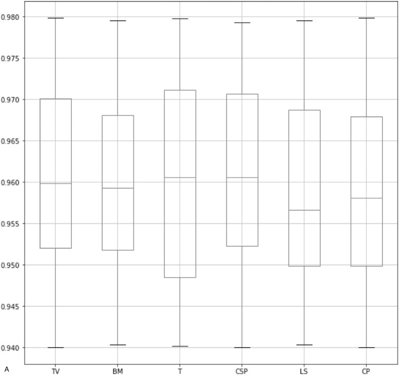
Box-plots of IoU values for 3 sections. The 3 lines on each box represent the 4 quartiles of the IoU values. IoU = intersection over union.

Table 4.

Comparisons about detection results between our method and other methods in head section.

Method	TV	BM	T	CP	CSP	LS	mAP
SSD	40.56	82.75	72.61	54.21	63.43	75.41	64.66
YOLOv2	35.43	79.31	38.56	62.70	83.67	83.31	63.83
Faster R-CNN VGG16	73.56	94.65	93.41	80.59	87.35	94.78	87.39
Faster R-CNN Resnet50	72.48	95.40	92.78	85.47	84.71	95.31	87.69
Lin	82.50	98.95	93.89	95.82	89.92	98.46	93.26
Non-NM	71.42	94.38	89.92	82.45	86.78	92.45	86.23
Our method	86.12	98.87	94.21	93.76	95.57	97.92	94.41

BM = brain midline, CP = choroid plexus, CSP = cavum septi pellucidi, LS = lateral sulcus, mAP = mean average precision, T = thalamus, TV = third ventricle.

Table 5.

Comparisons about detection results between our method and other methods in heart section.

Method	RV	RA	LV	LA	DAO	mAP
SSD	60.27	62.43	67.61	54.21	74.67	63.84
YOLOv2	71.31	69.39	71.56	62.70	90.74	73.14
Faster R-CNN VGG16	85.52	81.15	87.11	80.59	95.57	85.99
Faster R-CNN Resnet50	89.44	83.59	90.78	85.47	94.01	88.66
Non-NM	84.35	85.43	91.23	82.45	95.86	87.86
Our method	93.03	95.71	95.65	93.76	97.34	95.10

DAO = descending aorta, LA = left atrium, LV = left ventricle, mAP = mean average precision, RA = right atrium, RV = right ventricle.

Table 6.

Comparisons about detection results between our method and other methods in abdominal section.

Method	ST	UV	SP	AO	mAP
SSD	80.74	83.43	76.23	62.13	75.63
YOLOv2	88.21	85.47	78.61	67.71	80.00
Faster R-CNN VGG16	90.25	92.15	88.72	82.54	88.42
Faster R-CNN Resnet50	91.29	93.59	90.85	81.34	89.27
Non-NM	93.41	91.76	94.38	90.34	92.47
Our method	97.33	97.77	96.25	94.16	96.38

AO = aorta, mAP = mean average precision, SP = spine, ST = stomach, UV = umbilical vein.

3.4. Results of diagnosis accuracy

To illustrate the performance of our model in classifying the essential anatomical structures, we first use area of ROC and confusion matrix to characterize the performance of the classifier visually, then we use several authoritative indicators to measure it quantitatively: ACC, Spec, Sen, Pre, and F1. Also, to show the effectiveness of our proposed network in diagnosis, we have compared our method with other popular classification networks, including AlexNet,^[38] VGG16, VGG19,^[39] and ResNet50.^[40] The comparison with Lin's method is also carried out.

As shown in Figure 5, it is observed that the classifier achieves quite promising performance in all the 3 sections with the true positive rate reaching 100% while the false positive rate is less than 10%. Also, the ROC achieves at 0.96, 0.95, and 0.98 for the head section, abdominal section, and heart section, respectively.

Figure 4 (Continued).

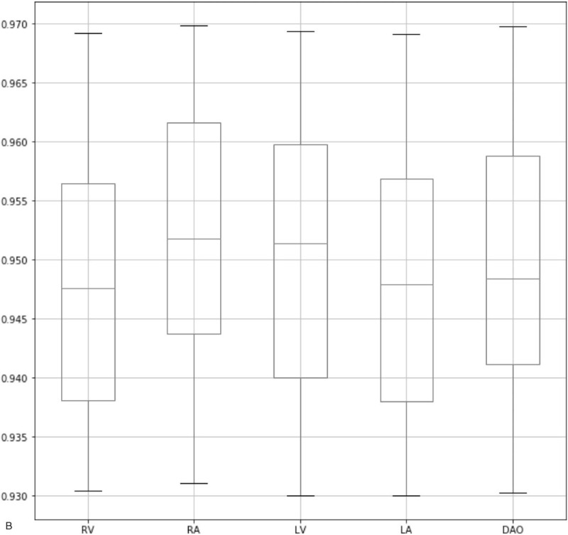
Box-plots of IoU values for 3 sections. The 3 lines on each box represent the 4 quartiles of the IoU values. IoU = intersection over union.

From Figure 6, it is clear that our method achieves a quite superior performance in every anatomical structure of different sections with the true positive rate reaching nearly 100%.

Figure 4 (Continued).

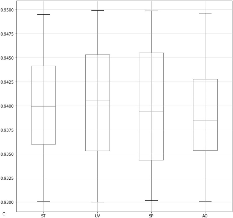
Box-plots of IoU values for 3 sections. The 3 lines on each box represent the 4 quartiles of the IoU values. IoU = intersection over union.

Figure 6.

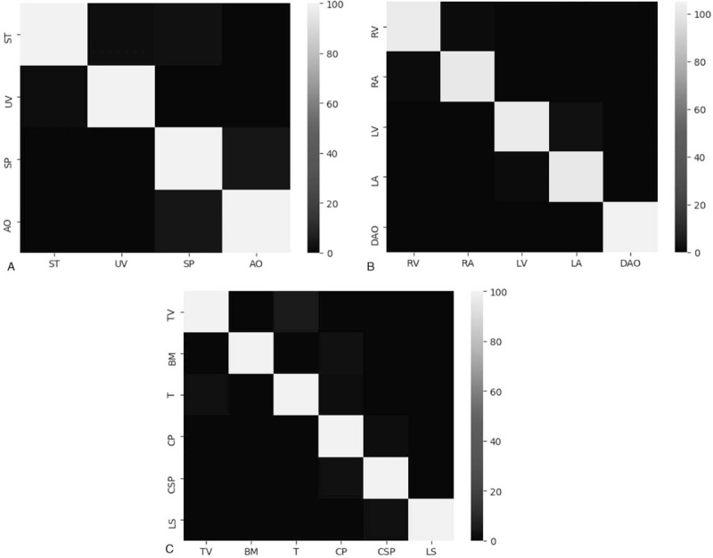
Confusion matrix of diagnosis methods. (A) represents abdominal section; (B) represents heart section; and (C) represents heart section.

From Table 7, we can observe that the classification results of our method are superior to other state-of-the-art methods. Specially, we achieve the best results with a precision of 94.63%, a specificity of 96.39%, and an AUC of 98.26%, which are better than Lin's method. The relative inferior results in sensitivity, accuracy, and F1-score can be further improved if we add prior clinical knowledge into our framework.^[16]Tables 8 and 9 illustrate the classification results in abdominal and heart section. We can observe that our method has achieved quite promising results in most indicators compared with existing methods. It demonstrates the effectiveness of our proposed method in classifying anatomical structures of all the sections.

Table 7.

Comparisons about classification results between our method and other methods in head section.

Indicator	Prec	Sen	ACC	F1	Spec	AUC
AlexNet	90.21	91.28	92.22	91.77	92.46	95.29
VGG16	92.34	92.48	91.79	90.68	93.71	96.37
VGG19	94.31	93.72	92.91	91.01	94.33	97.14
Resnet50	94.36	93.01	93.96	94.21	92.91	97.59
Lin	93.57	93.57	94.37	93.57	95.00	98.18
Our method	94.63	92.41	94.31	93.17	96.39	98.26

ACC = accuracy, AUC = the area under the receiver of operation curve, F1 = F1 score, Prec = precision, Sen = sensitivity, Spec = specificity.

Table 8.

Comparisons about classification results between our method and other methods in abdominal section.

Indicator	Prec	Sen	ACC	F1	Spec	AUC
AlexNet	91.34	91.24	92.11	90.43	91.53	93.12
VGG16	93.21	93.59	91.33	90.91	92.23	92.76
VGG19	93.42	94.27	92.12	93.91	92.91	93.21
Resnet50	94.52	94.10	93.66	93.76	95.92	96.32
Our method	95.67	93.56	96.31	93.17	97.92	98.54

ACC = accuracy, AUC = the area under the receiver of operation curve, F1 = F1 score, Prec = precision, Sen = sensitivity, Spec = specificity.

Table 9.

Comparisons about classification results between our method and other methods in heart section.

Indicator	Prec	Sen	ACC	F1	Spec	AUC
AlexNet	90.34	91.44	92.32	90.78	91.28	93.87
VGG16	92.76	93.71	92.13	93.12	92.33	93.43
VGG19	93.68	94.31	93.37	92.88	93.54	94.41
Resnet50	95.91	94.31	93.52	93.45	94.42	93.56
Our method	96.71	94.73	93.32	95.91	94.49	95.67

ACC = accuracy, AUC = the area under the receiver of operation curve, F1 = F1 score, Prec = precision, Sen = sensitivity, Spec = specificity.

3.5. Running time analysis and sensitivity analysis

We test the running time of detecting a single FS image for different single-task and multitask networks in a workstation equipped with 3.60 GHz Intel Xeon E5-1620 CPU and a GP106-100 GPU. The results are given in Table 10. It is observed that detecting a single frame could only cost 0.871s, which is fast enough to meet clinical needs. Also, it is observed that although the network parameters of our method and FLOPs are much more than Faster R-CNN + VGG16, there is not much difference in segmentation time, this is because our network shared many low-level features, which could achieve a more efficient segmentation with using only a few parameters.

Table 10.

The detection speed and parameters of different single-task and multitask methods.

Method	FLOPs (B)	Speed (s)	Parameters (M)
Single-task
AlexNet	0.71	0.012	61.10
VGG16	15.65	0.023	138.37
VGG19	19.82	0.025	143.68
ResNet50	4.12	0.052	22.56
YoLo v2	59.28	0.561	231.26
Multitask
Faster R-CNN VGG16	169.23	0.721	432.31
Our method	186.4	0.871	502.92

B = billion, FLOPs = floating point operations, M = million.

In the CNN model, we usually need to try a series of parameters to get the best performance for the model. There are many parameters that could affect the results of a CNN model such as learning rate, epoch, regularization loss, etc, but generally, the learning rate and weight decay have a great impact on it. Therefore, we change the learning rate and weight decay to illustrate the sensitivity of our method. As shown in Table 11, by altering the learning rate, the change of mAP does not exceed 1.7%; by changing the weight decay, the change of mAP does not exceed 2.2%, demonstrating the robustness of our method.

Table 11.

Comparisons about classification results between our method and other methods in abdominal section.

Learning rate	Epoch	Regularization loss	Weight decay	mAP
0.0000001	100	5	0.0001	95.1
0.000001	100	5	0.0001	93.4
0.00001	100	5	0.0001	94.8
0.0000001	100	5	0.0002	96.1
0.000001	100	5	0.0002	95.3
0.00001	100	5	0.0002	96.3
0.0000001	100	5	0.0003	94.7
0.000001	100	5	0.0003	93.3
0.00001	100	5	0.0003	94.1

mAP = mean average precision.

Figures 7–9 depict the comparison of our results with the manually labeled images by experts in the head section, abdominal section, and heart section, respectively. Our method displays the classification and segmentation results simultaneously to assist in sonographers’ observation. More comparison between our results and ground truth is given in Figure 10. It can be seen that our method is perfectly aligned with professional sonographers.

Figure 5.

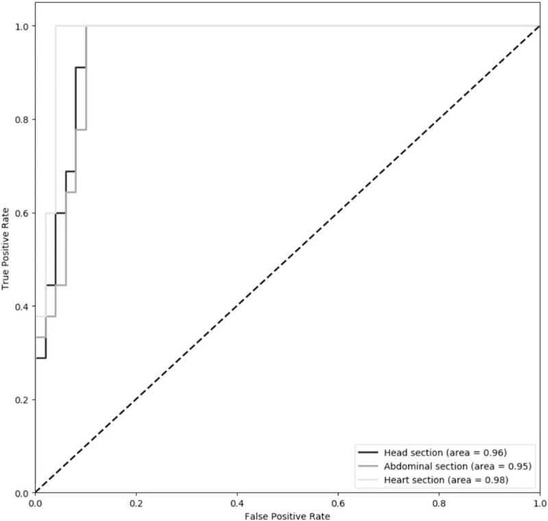
ROC curves of classification results in 3 sections. ROC = receiver operating characteristic.

Figure 7.

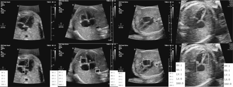
Demonstration that our results perfectly match with the annotations of ground truth in the heart section. The classification results in the left white box are the ground truth labeled by professional radiologists, and the results in the right white box are the detection results of our method. “1” means the anatomical structure meets the quality requirement, and “0” means the structure does not meet the requirement.

Figure 8.

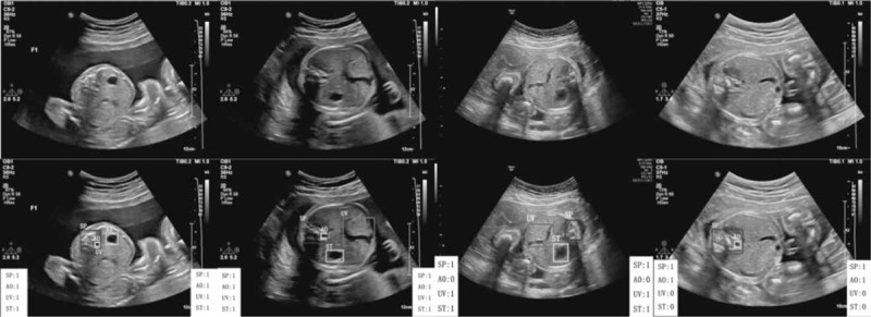
Demonstration that our results perfectly match with the annotations of ground truth in the abdominal section. The classification results in the left white box are the ground truth labeled by professional radiologists, and the results in the right white box are the detection results of our method. “1” means the anatomical structure meets the quality requirement, and “0” means the structure does not meet the requirement.

Figure 9.

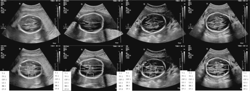
Demonstration that our results perfectly match with the annotations of ground truth in the head section. The classification results in the left white box are the ground truth labeled by professional radiologists, and the results in the right white box are the detection results of our method. “1” means the anatomical structure meets the quality requirement, and “0” means the structure does not meet the requirement.

Figure 10.

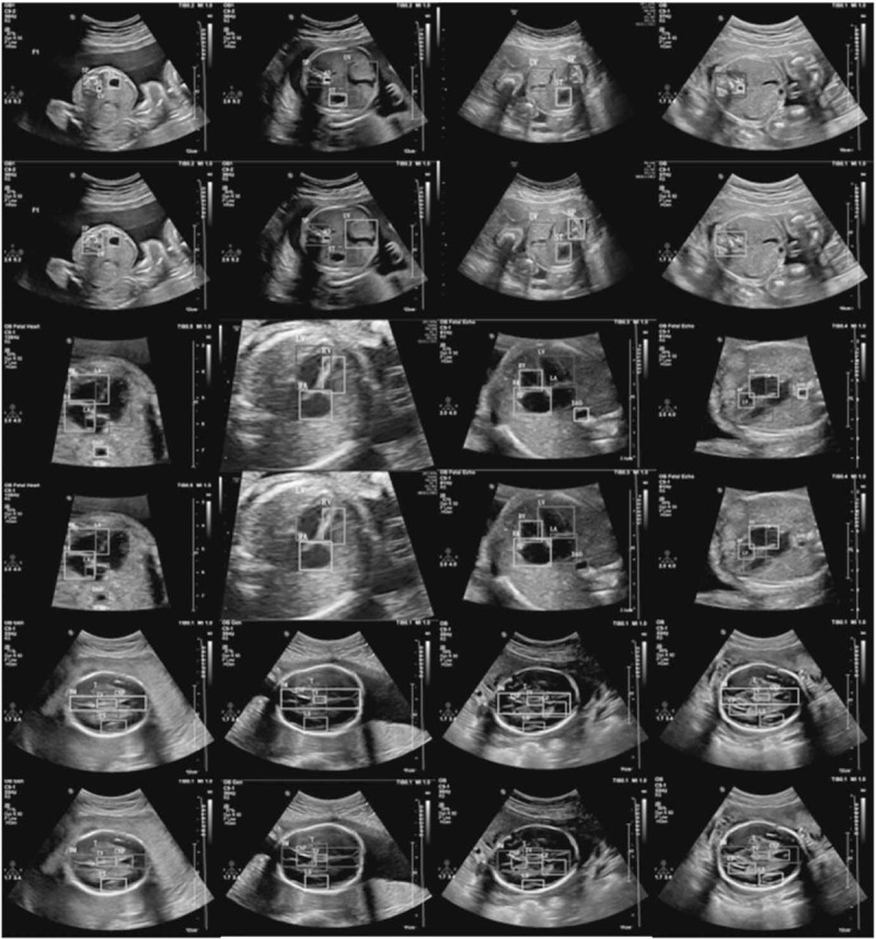
More comparisons between our results with ground truth. The first 2 rows show the results in the abdominal section, the middle 2 rows show the results in the heart section, and the last 2 rows show the results in the head section. For every section, the upper row represents the ground truth, and the lower row represents our results.

4. Discussion

In this paper, an autonomous image quality assessment approach for FS images was investigated. The experimental results show that our proposed scheme achieves a highly precise ROI localization and a considerable degree of accuracy for all the essential anatomical structures in the 3 standard planes. Also, the conformance test shows that our results are highly consistent with those of professional sonographers, and running time tests show that the image segmentation speed per frame is much higher than sonographers, which means this scheme can effectively replace the work of sonographers. In our proposed network, to further improve segmentation and classification accuracy, we also modify the recently published advanced object segmentation technologies and adapt them to our model. The experiment shows these modules are highly useful, and the overall performance is better than the state-of-the-art methods such as the FS image assessment framework proposed by Lin et al.^[16] After the Feature Extraction Network, we also divide the network into Region Proposal Network and Class Prediction Network. Accordingly, the features in the segmentation network can avoid interfering with the features in the classification network, so the segmentation accuracy is further increased. Also, the segmentation speed can be significantly improved, as the classification and localization are performed simultaneously.

Although our method achieves quite promising results, there are still some limitations. First, for the training sets, we regard the manually labeled FS images by 2 professional sonographers as the ground truth, but the results of manual labeling will have some accidental deviation even though they all have more than 10 years of experience. In future studies, we will invite more professional clinical expects to label the FS images and collect more representative datasets. Second, there still remain some segmentation and classification errors in our results. This is because our evaluation criteria are rigorous, and the midsection of a single anatomical structure could lead to a negative score on the image. Third, all the FS images are collected from GE Voluson E8 and Philips EPIQ 7 scanner; however, different types of ultrasonic instruments will produce different ultrasound images, which may cause our method not to be applied well to the FS images produced by other machines.

Our proposed method further boosts the accuracy in the assessment of two-dimensional FS standard plane. Although t3-dimensional and 4-dimensional ultrasound testing are popular recently, they are mainly utilized to meet the needs of pregnant women and their families to view baby pictures instead of serving the diagnosing purpose visually. Two-dimensional ultrasound images are still the most authoritative basis for judging fetal development.^[2] As illustrated before, there are still many challenges for the automatic assessment of 2D ultrasound images, such as shadowing effects, similar anatomical structures, different fetal positions, etc. To overcome these challenges and further promote the accuracy and robustness of segmentation and classification, it may be useful to add some prior clinical knowledge^[16] and more advanced attention modules to the network. In the future, we will also investigate the automatic selection technology for finding the standard scanning plane, which will find a standard plane containing all the essential anatomical structures without sonographers’intervention.

Acknowledgments

The authors acknowledge Sichuan University West China Second Hospital for providing the fetal ultrasound image datasets.

Author contributions

Conceptualization: Bo Zhang, Hong Luo.

Data curation: Bo Zhang, Hong Luo.

Formal analysis: Bo Zhang, Hong Luo.

Funding acquisition: Hong Luo.

Investigation: Bo Zhang, Kejun Li.

Methodology: Bo Zhang, Han Liu, Kejun Li.

Project administration: Hong Luo.

Resources: Hong Luo.

Software: Bo Zhang, Han Liu.

Supervision: Hong Luo.

Validation: Han Liu.

Visualization: Han Liu.

Writing – original draft: Han Liu.

Writing – review & editing: Bo Zhang, Han Liu, Kejun Li.

Glossary

Abbreviations: ACC = accuracy, AP = average precision, AUC = area under the receiver of operation curve, BSI = biometry suitability index, CNN = Convolutional Neural Network, CPN = class prediction network, F1 = F1-score, FC = fully connected, FEN = feature extraction network, FLOPs = floating point operations, FPN = feature pyramid network, FS = fetal sonographic, GAP = global average pooling, IoU = Intersection over Union, mAP = mean average precision, MSP = mid-sagittal plane, Pre = precision, ROC = receiver operating characteristic (ROC), ROI = region of interest, RPN = region proposal network, Sen = sensitivity, Spec = specificity, SPP = spatial pyramid pooling.

References

- [1].Rueda S, Fathima S, Knight CL, et al. Evaluation and comparison of current fetal ultrasound image segmentation methods for biometric measurements: a grand challenge. IEEE Trans Med Imaging 2014;33:797–813. [DOI] [PubMed] [Google Scholar]
- [2].American Institute of Ultrasound in Medicine. AIUM practice guideline for the performance of obstetric ultrasound examinations. J Ultrasound Med 2013;32:1083–101. [DOI] [PubMed] [Google Scholar]
- [3].Chambers SE, Muir BB, Haddad NG. Ultrasound evaluation of ectopic pregnancy including correlation with human chorionic gonadotrophin levels. Br J Radiol 1990;63:246–50. [DOI] [PubMed] [Google Scholar]
- [4].Hill LM, Kislak S, Martin JG. Transvaginal sonographic detection of the pseudogestational sac associated with ectopic pregnancy. Obstet Gynecol 1990;75:986–8. [PubMed] [Google Scholar]
- [5].Barnhart K, Van Mello NM, Bourne T, et al. Pregnancy of unknown location: a consensus statement of nomenclature, definitions, and outcome. Fertil Steril 2011;95:857–66. [DOI] [PMC free article] [PubMed] [Google Scholar]
- [6].Jeve Y, Rana R, Bhide A, et al. Accuracy of first-trimester ultrasound in the diagnosis of early embryonic demise: a systematic review. Ultrasound Obstet Gynecol 2011;38:489–96. [DOI] [PubMed] [Google Scholar]
- [7].Thilaganathan B. Opinion: The evidence base for miscarriage diagnosis: better late than never. Ultrasound Obstet Gynecol 2011;38:487–8. [DOI] [PubMed] [Google Scholar]
- [8].Murphy SL, Xu J, Kochanek KD, et al. Mortality in the United States, 2017: key findings data from the national vital statistics system 2018;1–8. [Google Scholar]
- [9].Zhang L, Dudley NJ, Lambrou T, et al. Automatic image quality assessment and measurement of fetal head in two-dimensional ultrasound image. J Med Imaging 2017;4:024001. [DOI] [PMC free article] [PubMed] [Google Scholar]
- [10].Ghesu FC, Krubasik E, Georgescu B, et al. Marginal space deep learning: efficient architecture for volumetric image parsing. IEEE Trans Med Imaging 2016;35:1217–28. [DOI] [PubMed] [Google Scholar]
- [11].Zhang J, Liu M, Shen D. Detecting anatomical landmarks from limited medical imaging data using two-stage task-oriented deep neural networks. IEEE Trans Image Process 2017;26:4753–64. [DOI] [PMC free article] [PubMed] [Google Scholar]
- [12].Ghesu FC, Georgescu B, Zheng Y, et al. Multi-scale deep reinforcement learning for real-time 3D-landmark detection in CT scans. IEEE Trans Pattern Anal Mach Intell 2019;41:176–89. [DOI] [PubMed] [Google Scholar]
- [13].Kebir ST, Mekaoui S. An Efficient Methodology of Brain Abnormalities Detection using CNN Deep Learning Network. In: Proceedings of the 2018 International Conference on Applied Smart Systems, ICASS 2018. [Google Scholar]
- [14].Sujit SJ, Gabr RE, Coronado I, et al. Automated Image Quality Evaluation of Structural Brain Magnetic Resonance Images using Deep Convolutional Neural Networks. In: 2018 9th Cairo International Biomedical Engineering Conference, CIBEC 2018 - Proceedings 2019;33–6. [Google Scholar]
- [15].Deepika P, Suresh RM, Pabitha P. Defending against child death: deep learning-based diagnosis method for abnormal identification of fetus ultrasound Images. Comput Intell 2020;1:1–27. [Google Scholar]
- [16].Lin Z, Li S, Ni D, et al. Multi-task learning for quality assessment of fetal head ultrasound images. Med Image Anal 2019;58:101548. [DOI] [PubMed] [Google Scholar]
- [17].Xu Z, Huo Y, Park JH, et al. Less is more: Simultaneous view classification and landmark detection for abdominal ultrasound images. In: Lecture Notes in Computer Science (Including Subseries Lecture Notes in Artificial Intelligence and Lecture Notes in Bioinformatics). Vol 11071 LNCS. Springer Verlag; 2018:711–719. [Google Scholar]
- [18].Wu L, Cheng JZ, Li S, et al. FUIQA: fetal ultrasound image quality assessment with deep convolutional networks. IEEE Trans Cybern 2017;47:1336–49. [DOI] [PubMed] [Google Scholar]
- [19].Institute of Electrical and Electronics Engineers Inc., Chang CW, Huang ST, Huang YH, et al. Categorizating 3d fetal ultrasound image database in first trimester pregnancy based on mid-sagittal plane assessments. In: Proceedings Applied Imagery Pattern Recognition Workshop. Vol 2017. 2018. [Google Scholar]
- [20].Kumar AMC, Shriram KS. Automated scoring of fetal abdomen ultrasound scan-planes for biometry. In: Proceedings International Symposium on Biomedical Imaging Vol 2015 2015;862–5. [Google Scholar]
- [21].Baumgartner CF, Kamnitsas K, Matthew J, et al. SonoNet: real-time detection and localisation of fetal standard scan planes in freehand ultrasound. IEEE Trans Med Imaging 2017;36:2204–15. [DOI] [PMC free article] [PubMed] [Google Scholar]
- [22].Namburete AIL, Xie W, Yaqub M, et al. Fully-automated alignment of 3D fetal brain ultrasound to a canonical reference space using multi-task learning. Med Image Anal 2018;46:1–4. [DOI] [PubMed] [Google Scholar]
- [23].Ren S, He K, Girshick R, et al. Faster R-CNN: towards real-time object detection with region proposal networks. IEEE Trans Pattern Anal Mach Intell 2017;39:1137–49. [DOI] [PubMed] [Google Scholar]
- [24].Zhao Z, Liu H, Fingscheidt T. Convolutional neural networks to enhance coded speech. IEEE/ACM Trans Audio Speech Lang Process 2019;27:663–78. [Google Scholar]
- [25].Dai J, Li Y, He K, Sun J. R-FCN: Object detection via region-based fully convolutional networks. In: Advances in Neural Information Processing Systems; 2016:379–387. Available at: https://github.com/daijifeng001/r-fcn. Accessed October 26, 2019. [Google Scholar]
- [26].Lin M, Chen Q, Yan S. Network in network. In: 2nd International Conference on Learning Representations, ICLR 2014 - Conference Track Proceedings 2014. [Google Scholar]
- [27].Hu H, Gu J, Zhang Z, et al. Relation Networks for Object Detection. In: Proceedings of the IEEE Computer Society Conference on Computer Vision and Pattern Recognition 2018;3588–97. [Google Scholar]
- [28].He K, Zhang X, Ren S, et al. Spatial pyramid pooling in deep convolutional networks for visual recognition. IEEE Trans Pattern Anal Mach Intell 2015;37:1904–16. [DOI] [PubMed] [Google Scholar]
- [29].He K, Zhang X, Ren S, et al. Identity mappings in deep residual networks. In: Lecture Notes in Computer Science (Including Subseries Lecture Notes in Artificial Intelligence and Lecture Notes in Bioinformatics) 2016. [Google Scholar]
- [30].Lin TY, Dollár P, Girshick R, et al. Feature pyramid networks for object detection. In: Proceedings 30th IEEE Conference on Computer Vision and Pattern Recognition, CVPR 2017. [Google Scholar]
- [31].Lin TY, Goyal P, Girshick R, et al. Focal loss for dense object detection. IEEE Trans Pattern Anal Mach Intell 2020;42:318–27. [DOI] [PubMed] [Google Scholar]
- [32].Fawcett T. An introduction to ROC analysis. Pattern Recognit Lett 2006;27:861–74. [Google Scholar]
- [33].Sokolova M, Lapalme G. A systematic analysis of performance measures for classification tasks. Inf Process Manag 2009;45:427–37. [Google Scholar]
- [34].Hunger R. Floating point operations in matrix-vector calculus. Tech Univ München 2007. [Google Scholar]
- [35].Liu W, Anguelov D, Erhan D, et al. SSD: single shot multibox detector. In: Lecture Notes in Computer Science (Including Subseries Lecture Notes in Artificial Intelligence and Lecture Notes in Bioinformatics) 2016. [Google Scholar]
- [36].Redmon J, Divvala S, Girshick R, et al. You only look once: unified, real-time object detection. In: Proceedings of the IEEE Computer Society Conference on Computer Vision and Pattern Recognition 2016. [Google Scholar]
- [37].Redmon J, Farhadi A. YOLO9000: Better, Faster, Stronger. Available at: http://pjreddie.com/yolo9000/. Accessed October 27, 2019. [Google Scholar]
- [38].Krizhevsky A, Sutskever I, Hinton GE. ImageNet classification with deep convolutional neural networks. In: Advances in Neural Information Processing Systems 2012. [Google Scholar]
- [39].Simonyan K, Zisserman A. Very deep convolutional networks for large-scale image recognition. 2014:1–14. Available at: http://arxiv.org/abs/1409.1556. Accessed April 10, 2015. [Google Scholar]
- [40].He K, Zhang X, Ren S, Sun J. Deep residual learning for image recognition. In: Proceedings of the IEEE Computer Society Conference on Computer Vision and Pattern Recognition; 2016. [Google Scholar]