The Added Value of New Covariates to the Brier Score in Cox Survival Models

Abstract

Calibration is an important measure of the predictive accuracy for a prognostic risk model. A widely used measure of calibration when the outcome is survival time is the expected Brier score. In this paper, methodology is developed to accurately estimate the difference in expected Brier scores derived from nested survival models and to compute an accompanying variance estimate of this difference. The methodology is applicable to time invariant and time-varying coefficient Cox survival models. The nested survival model approach is often applied to the scenario where the full model consists of conventional and new covariates and the subset model contains the conventional covariates alone. A complicating factor in the methodologic development is that the Cox model specification cannot, in general, be simultaneously satisfied for nested models. The problem has been resolved by projecting the properly specified full survival model onto the lower dimensional space of conventional markers alone. Simulations are performed to examine the method’s finite sample properties and a prostate cancer data set is used to illustrate its application.

1. Introduction

Risk modeling has emerged as an area of significant interest in clinical research. The models have a direct impact on patient treatment and health. As examples, physicians use them to identify which patients are candidates for further diagnostic testing, such as surgical biopsy; they are also used to assess the likelihood of clinical outcomes, such as response to treatment or survival. Due to the complexity of understanding disease etiology, risk models include a combination of risk factors, with new risk factors continually introduced. The utility of these updated models is a function of their predictive accuracy, which include measures of calibration, discrimination, and explained variation. In this work, the prognostic utility of a set of new risk factors will be evaluated by a calibration measure for survival models.

Measures of calibration for survival data are often generated through loss functions that are applied to point prediction and survival status prediction (Lawless and Yuan 2010). Loss functions used to produce calibration measures for survival data include: absolute error (Tian et al. 2007, Schemper 1990), entropy (Korn and Simon 1990), missclassification error (Uno et al. 2007), and squared error (Graf et al. 1999, Gerds and Schumacher 2007). An alternative statistic that has gained recent popularity is calibration in the large, which may be measured as the ratio of the Kaplan-Meier estimate at a given time point to the average model-based predicted survival probability (Demler et al. 2015).

In this paper, the focus is on a widely used measure of calibration: the expected Brier score, a mean squared error loss function. The expected Brier score evaluated at time t is defined as

$$E\left[B\left(t\right)\right]=E{\left[I\left(T>t\right)-S_t\left(\mathit{X},\mathit{Z}\right)\right]}^2,$$

where T is the survival time random variable, S_t(X, Z) represents a model based predicted probability of surviving beyond time t for the conventional risk factors X and a set of new risk factors to be added to the survival model Z, and the expectation is with respect to (T, X, Z). In addition, the random censoring times are denoted by C and the observed survival times by Y = min(T, C). It is assumed the T and C are independent conditional on (X, Z). Throughout the paper, capital letters indicate random variables, lower case letters represent their observations, and bold type designates vectors. An important property of the Brier score is that it is a proper score (Gneiting and Raftery 2007), implying that the expected Brier score is minimized when the survival predictor S_t(X, Z) is correctly specified and is equal to E[I(T > t)|X, Z].

A framework is developed to assess the effect of new risk factors (Z) on the expected Brier score. For the analyst with a dataset, the first step is to develop a survival model that adequately fits the data containing the covariates (x, z). The Cox model with time-varying coefficients is a flexible risk model for survival and is characterized by the property that the covariates are an additive function of the log negative log survival function. The Cox survival function at time t, for an individual with covariates (x, z), may be defined as (Peng and Huang 2007)

$$S_t\left(\mathit{x},\mathit{z}\right)=\exp \left\{-\exp \left[{\alpha }_t+{\mathit{\beta }}_t^T\mathit{x}+{\mathit{\gamma }}_t^T\mathit{z}\right]\right\}.$$ (1)

The estimated survival function is computed using an estimating equation approach, where Peng and Huang (2007) demonstrate that the time-varying coefficient estimates $\left({\widehat{\mathit{\alpha }}}_t,{\widehat{\mathit{\beta }}}_t,{\widehat{\mathit{\gamma }}}_t\right)$ are $\sqrt{n}$ consistent and asymptotically normal. An alternative definition of the Cox survival function, which is defined through a time-varying coefficient hazard function, is derived in Cai and Sun (2003) and Tian et al. (2005). In practice, the most frequently applied Cox model is the proportional hazards model; a special case of the time-varying coefficient model with β_t = β and γ_t = γ and α_t is the log baseline cumulative hazard function.

A popular estimate of the decrement in the expected Brier score, due to the introduction of new factors to the survival model, is the difference in the observed Brier scores (Graf et al. 1999, Gerds and Schumacher 2007)

$$n^{-1}\sum _i{w}_i\left(t;\widehat{G}\right){\left[I\left(Y_i>t\right)-{\widehat{R}}_t\left({\mathit{x}}_i\right)\right]}^2-n^{-1}\sum _i{w}_i\left(t;\widehat{G}\right){\left[I\left(Y_i>t\right)-{\widehat{S}}_t\left({\mathit{x}}_i,{\mathit{z}}_i\right)\right]}^2,$$ (2)

where i indexes independent subjects, ${\widehat{R}}_t\left(\mathit{x}\right)$ represents a working time-varying coefficient Cox survival model

$${\widehat{R}}_t\left(\mathit{x}\right)=\exp \left\{-\exp \left[{\widehat{\alpha }}_t^{*}+{\widehat{\beta }}_t^{*T}\mathit{x}\right]\right\},$$ (3)

estimated using x alone, $w_i\left(t;\widehat{G}\right)$ is the inverse probability censoring weight (IPCW)

$$w_i\left(t;\widehat{G}\right)=\frac{I\left[Y_i\hspace{0.17em}\le \hspace{0.17em}t,T_i\hspace{0.17em}<\hspace{0.17em}{C}_i\right]}{\widehat{G}\left(Y_i^{-}\right)}+\frac{I\left[Y_i\hspace{0.17em}>\hspace{0.17em}t\right]}{\widehat{G}\left(t\right)},$$

and $\widehat{G}$ is the Kaplan-Meier estimate of the censoring time C survival function. If the censoring distribution is a function of the covariates, then an estimated survival function of the censoring time conditional on the covariates should be used.

An underappreciated problem with this approach is that Cox models are not, in general, closed under nesting. Thus, if the survival function is modelled using the time-varying coefficient Cox model (1), the survival function based on x alone is typically not a member of this family. As noted in the frailty literature, the only case where the Cox model is closed under nesting is when the random variable $\exp \left({\mathit{\gamma }}_t^T\mathit{Z}\right)$ follows a positive stable distribution (Hougaard 1986).

Applied statisticians are aware of the non-nesting issue with nonlinear risk models, but for the purposes of application cite the George E.P. Box dictum, ”essentially, all models are wrong, but some are useful” (Box and Draper, 1987). Although this may be true, particularly in cases where the new factors provide little added value, the working nested time-varying coefficient Cox survival model (3) will produce an inconsistent estimate for the difference in the expected Brier score, which may lead to an erroroneous conclusion regarding the prognostic utility of the new factors (Rosthoj and Keiding 2004). A supporting issue, which stems from the non-nesting property and the proper scoring principle, is that an incorrectly specified working nested survival model does not minimize the expected Brier score. This can lead to an overvaluation of the added value of the new factors (z) when using the difference in the expected Brier scores.

To address the non-nesting problem, methodology is developed in Section 2 for estimation and inference of this difference using only the time varying coefficient survival model S_t(x, z) defined in (1). Section 3 assesses its finite sample properties through simulation. Section 4 applies the methodology to evaluate new biomarkers for patients with metastatic prostate cancer and Section 5 concludes the paper with a discussion.

2. The added value of new factors to the expected Brier score

Assume that after the implementation of diagnostics, the analyst is satisfied that the survival model containing (x, z) is properly specified using either a time-varying coefficient or a time invariant Cox model. From a practical viewpoint, this will often include the application of graphical procedures and goodness of fit tests, such as those developed by Grambsch and Therneau (1994), Martinussen and Scheike (2006), Peng and Huang (2007), Tian et al.(2005).

Denote the true conditional survival probabilities as

$${\pi }_t\left(\mathit{x},\mathit{z}\right)\equiv \mathrm{Pr}\left(T>t|\mathit{x},\mathit{z}\right)\hspace{1em}{\pi }_t\left(\mathit{x}\right)\equiv \mathrm{Pr}\left(T>t|\mathit{x}\right).$$

Although the survival model S_t(x, z) may be used to estimate π_t(x, z), estimation of π_t(x) is less straightforward due to the non-nesting issue. Using projection theory, S_t(X, Z) is the projection of I(T > t) onto the Hilbert space of random variables $\mathcal{H}\left(X,Z\right)$ and

$${\pi }_t\left(\mathit{X}\right)=E_{\mathit{Z}}\left[S_t\left(\mathit{X},\mathit{Z}\right)|\mathit{X}\right]$$ (4)

is the projection of S_t(X, Z) onto the subspace $\mathcal{H}\left(\mathit{X}\right)$ (Figure 1). Employing this projection, the difference in the expected Brier scores at time t may be computed using only S_t(X, Z). The expected difference in Brier scores due to the inclusion of Z is

$${\Delta }^2\left(t;{\mathit{\theta }}_t\right)=E{\left\{I\left(T>t\right)-{\pi }_t\left(\mathit{X}\right)\right\}}^2-E{\left\{I\left(T>t\right)-S_t\left(\mathit{X},\mathit{Z}\right)\right\}}^2,$$

where θ_t = (α_t, β_t, γ_t), and application of the Pythagorean Theorem and the law of iterated expectation provides the simplification

$${\Delta }^2\left(t;{\mathit{\theta }}_t\right)=E{\left\{{\pi }_t\left(\mathit{X}\right)-S_t\left(\mathit{X},\mathit{Z}\right)\right\}}^2.$$ (5)

To estimate this change in the expected Brier score, the conditional expectation (4) is estimated through kernel smoothing

$${\widehat{\pi }}_t\left(\mathit{X}\right)=\frac{{\sum }_j{\widehat{S}}_t\left(\mathit{x},{\mathit{z}}_j\right)K_h\left({\widehat{\mathit{\beta }}}_t^T\mathit{x},{\widehat{\mathit{\beta }}}_t^T{\mathit{x}}_j\right)}{{\sum }_j{K}_h\left({\widehat{\mathit{\beta }}}_t^T\mathit{x},{\widehat{\mathit{\beta }}}_t^T{\mathit{x}}_j\right)}$$ (6)

where K is a univariate kernel function with bandwidth h and j indexes subjects. Since the full model is properly specified, the survival information at time t is contained in the risk score and the utilization of the linear combination of covariates within the kernel enable avoidance of the curse of dimensionality when projecting onto the lower dimensional space (Horowitz 1998). Hence, the change in the expected Brier score may be estimated as

$$D_n^2\left(t;{\widehat{\mathit{\theta }}}_t\right)=n^{-1}{\sum _i\left[\frac{{\sum }_j{\widehat{S}}_t\left({\mathit{x}}_i,{\mathit{z}}_j\right)K_h\left({\widehat{\mathit{\beta }}}_t^T{\mathit{x}}_i,{\widehat{\mathit{\beta }}}_t^T{\mathit{x}}_j\right)}{{\sum }_j{K}_h\left({\widehat{\mathit{\beta }}}_t^T{\mathit{x}}_i,{\widehat{\mathit{\beta }}}_t^T{\mathit{x}}_j\right)}-{\widehat{S}}_t\left({\mathit{x}}_i,{\mathit{z}}_i\right)\right]}^2,$$ (7)

where ${\widehat{\mathit{\theta }}}_t=\left({\widehat{\alpha }}_t,{\widehat{\mathit{\beta }}}_t,{\widehat{\mathit{\gamma }}}_t\right)$.

FIGURE 1.

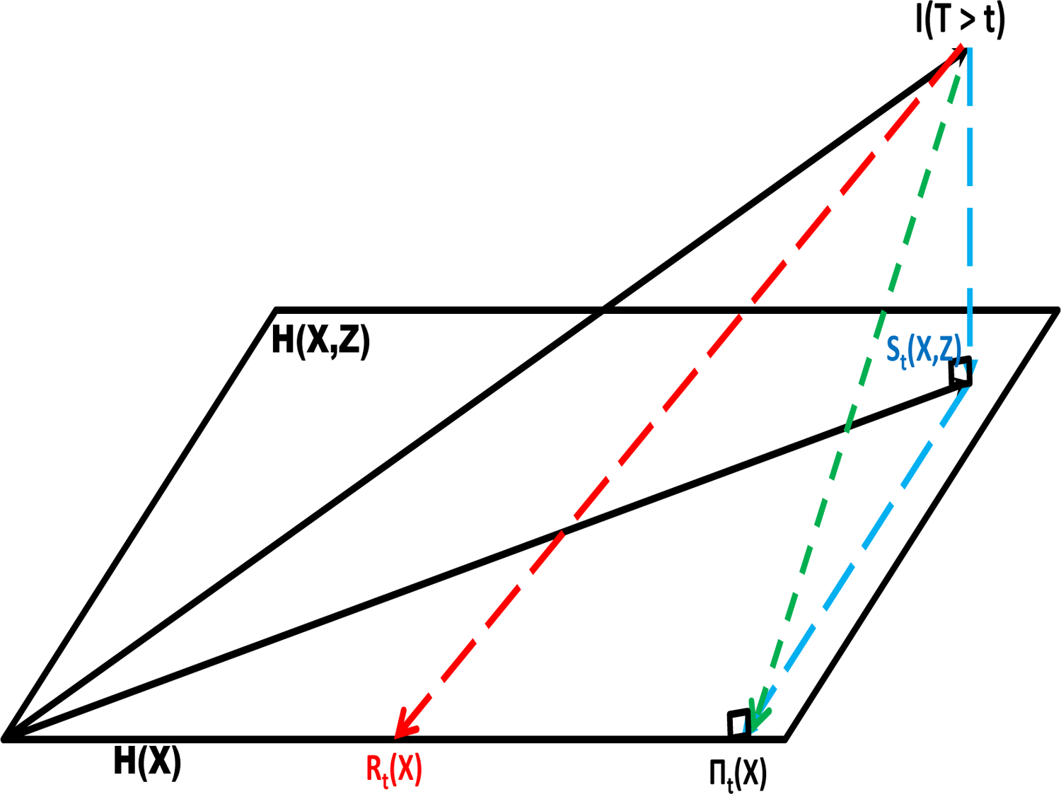
The projection of the random variable I(T > t) onto the Hilbert space H(X, Z) resulting in the random survival function S_t(X, Z) and its projection onto the subspace H(X) resulting in the random survival function π_t(X). R_t(X) is the working misspecified survival function in H(X).

A challenging issue with the Brier score is the interpretation of its scale. However, for the difference in Brier scores, the squared distance metric between the two survival functions in (5) may provide a gauge as to what constitutes a meaningful decrement in the expected Brier score due to the addition of the new factors. Borrowing from the equivalence methodology in comparative clinical trial research, one may consider that at a given time point, an absolute difference in population survival probabilities less than δ constitutes equivalence (Wellek 1993). As a result, going forward, the statistic used for evaluation is $D_n\left(t;{\widehat{\mathit{\theta }}}_t\right)=\sqrt{D_n^2\left(t;{\widehat{\mathit{\theta }}}_t\right)}$ and the parameter $\Delta \left(t;{\mathit{\theta }}_t\right)=\sqrt{{\Delta }^2\left(t;{\mathit{\theta }}_t\right)}$, which represents the distance between the two survival functions.

The choice of δ will differ depending on context. For large cardiovascular observational studies, δ may be as small as 0.05, whereas for smaller oncology studies, this threshold may be somewhat larger. Although ad-hoc, this use of an equivalence threshold may be appropriated to determine a meaningful improvement in the square root of the expected difference in Brier scores.

This type of thresholding may be used in conjunction with the variability of the estimate to evaluate the added value of the new factors to the Cox model. The variability is derived from the asymptotic distribution of the estimated difference in the expected Brier scores, which is stated below.

Theorem:

Assume the time-varying coefficient model based on the covariates (x, z) is properly specified in (1) and the new factors are associated with survival time $\left({\gamma }_t\ne 0\right)$. Then $\sqrt{n}\left[D_n\left(t;{\widehat{\mathit{\theta }}}_t\right)-\Delta \left(t;{\mathit{\theta }}_t\right)\}\right]$ converges in distribution, pointwise in t, to N [0, V].

The derivation is provided in the appendix. The asymptotic variance and corresponding confidence interval are computed using the bootstrap. The validity of the bootstrap in semiparametric models was established in Kosorok et al. (2004). If (1) reduces to the time-invariant coefficient proportional hazards model, the asymptotic normality of the estimated difference in the expected Brier scores follows directly from this derivation, replacing $\left({\widehat{\alpha }}_t,{\widehat{\mathit{\beta }}}_t,{\widehat{\mathit{\gamma }}}_t\right)$ with the estimates $\left(\log \left({\widehat{H}}_{0t}\right),\widehat{\mathit{\beta }},\widehat{\mathit{\gamma }}\right)$ derived from the time invariant coefficient partial likelihood, where H_0t denotes the baseline cumulative hazard function. Note that the baseline cumulative hazard and time invariant coefficient estimates converge to normality at the same $\sqrt{n}$ rate as the time-varying coefficients derived in Peng and Huang (2007).

The pointwise convergence of D_n(t) to asymptotic normality is slower as ∆(t) nears the boundary zero. This will be manifest in the positive relationship between D_n(t) and var(D_n(t)). To address this issue, a stabilizing square root transformation is applied to compute a confidence interval for ∆(t) (DiCiccio et al. 2006). For $C_n(t) = \sqrt{D_n(t)}$, the asymptotic 95% confidence interval for ∆(t), based on a back transformation of the square root transformation is,

$$\left({\left\{C_n\left(t\right)-1.96\sqrt{\mathrm{var}\left(C_n\left(t\right)\right)}\right\}}^2,{\left\{C_n\left(t\right)+1.96\sqrt{\mathrm{var}\left(C_n\left(t\right)\right)}\right\}}^2\right).$$

If $C_n\left(t\right)-1.96\sqrt{\mathrm{var}\left(C_n\left(t\right)\right)}$ is negative, then the lower confidence bound is set to zero.

3. Simulations

3.1. Properly specified time-varying coefficient Cox model

A mixed time-varying coefficient Cox model survival function

$$S_t\left(\mathit{x},z\right)=\exp \left\{-\exp \left[{\alpha }_t+{\beta }_{1t}{x}_1+{\beta }_{2t}{x}_2+\gamma z\right]\right\}$$ (8)

was used to compute the square root of the expected difference in Brier scores (5). To estimate π_t(x) in (4), the projection method (6) and a working (misspecified) time-varying coefficient Cox survival function (3) were evaluated.

Conditional on the covariates, the survival times from (8) were generated from a Weibull random variable with shape parameters ν = {0.5, 1.0, 2.0} and scale parameters λ, which were selected to produce a square root difference in expected Brier score equal to ∆(t; θ_t) = {0.05, 0.10, 0.15}, at t = 12. The time-varying regression coefficients were set equal to (β₁ log t, β₂ log t), with β₁ = β₂ = 1, and (x₁, x₂) were independent unit exponentials. The time-invariant component, exp(γz) was generated from a gamma random variable with parameters (ϕ, ϕ). The gamma specification, with equal shape and scale parameters, was used to take advantage of the existing literature on unobserved heterogeneity using a gamma frailty. Specifically under (8),

$${\pi }_t(\mathit{x})={\left(\frac{\varphi }{\varphi +\lambda t^{\nu +{\beta }_1{x}_1+{\beta }_2{x}_2}}\right)}^{\varphi }$$

(Kosorok, Lee, and Fine, 2004), enabling an analytic evaluation of the difference in the expected Brier scores. The gamma parameters used in the simulation were ϕ = {0.75, 1.333}.

The censoring distribution was uniform, independent of (x, z), with parameters chosen to produce average censoring proportions of {0, 0.25, 0.50, 0.75}. The bandwidth for the Gaussian kernel used to estimate π_t(x) in the projection method was ${\widehat{\sigma }}_{xt}{n}^{-0.126}$, which satisfies the condition nh⁸ → 0, indicated in the appendix, and ${\widehat{\sigma }}_{xt}$ is the estimated standard deviation of ${\widehat{\mathit{\beta }}}_t^T\mathit{x}$. The bootstrap was used to compute the asymptotic variance of the estimates along with asymptotic 95% confidence intervals. The sample size for each simulation was 300, with 500 simulations for each parameter combination evaluation (4 censoring proportions, 3 square root difference in expected Brier scores, 3 Weibull shape parameters, and 2 gamma frailty parameters). A summary of the results, based on the 72 parameter combinations is provided in the next paragraph and Figures 2–4; the individual results are given Supplemental Tables 1 and 2.

FIGURE 2.

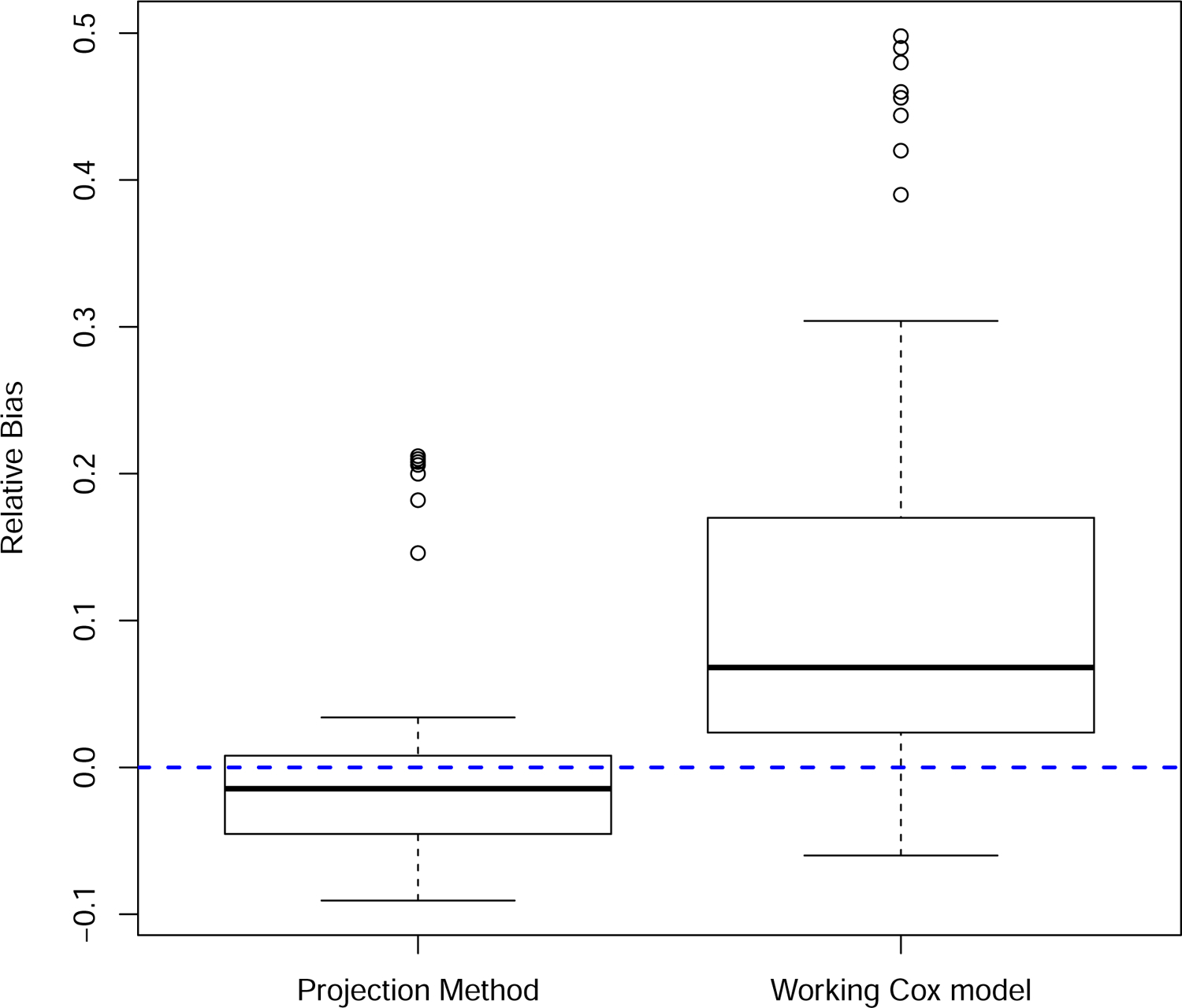
Relative bias in the square root estimated difference in the expected Brier scores. Results from the 72 parameter combinations specified in Section 3.

FIGURE 4.

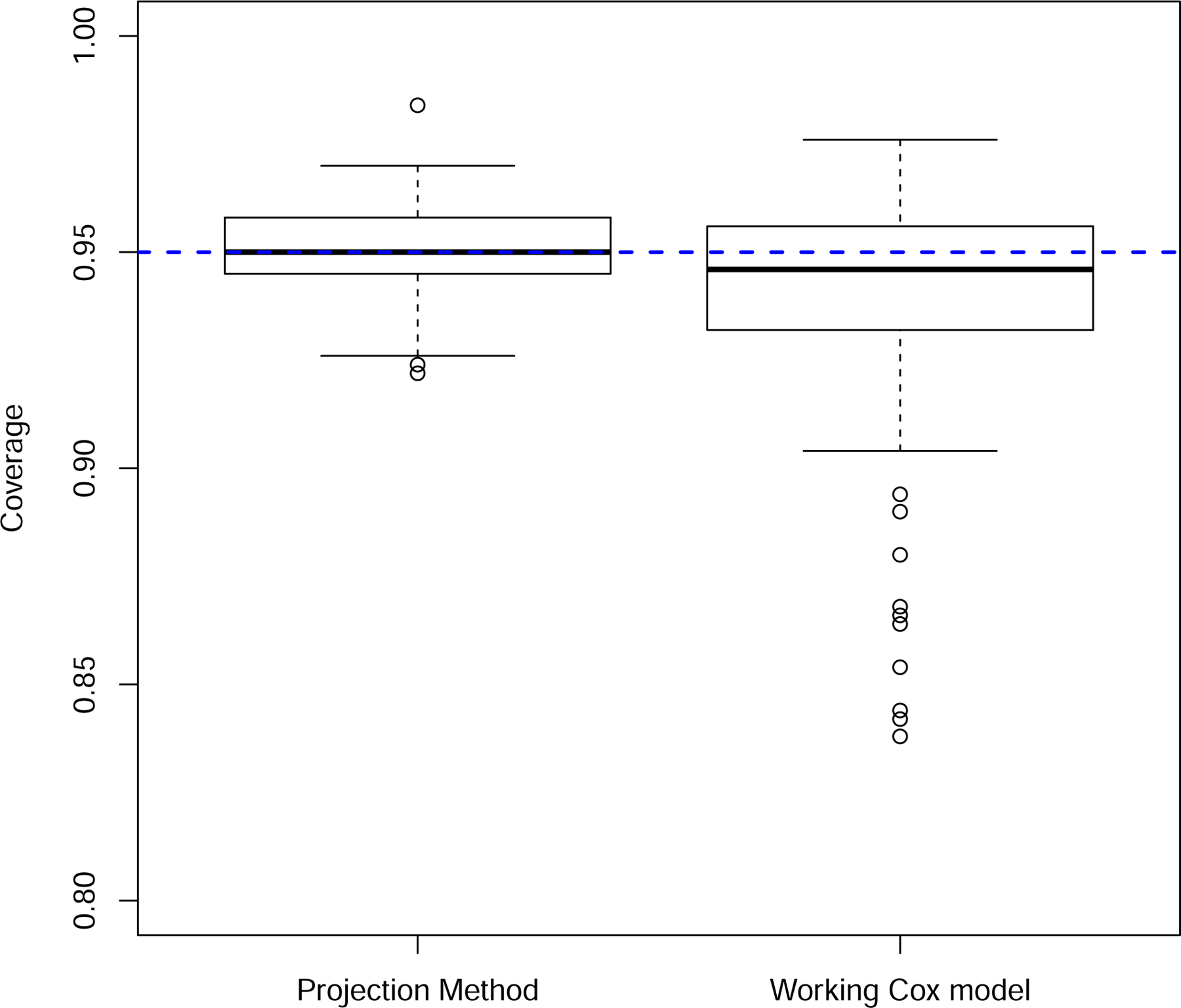
Coverage probabilities from 95% confidence intervals. Results from the 72 parameter combinations specified in Section 3.

The projection method was accurate, with a mean relative bias equal to −0.001 and standard deviation equal to 0.075. In contrast, the relative bias in the difference in observed Brier scores was positive (mean = 0.119, sd = 0.151), providing empirical corroboration of the overvaluation of the new markers using this approach (Figure 2). The projection method also provided accurate bootstrap standard error estimates relative to the observed Brier score method, which overestimated the variability in the estimated difference in the expected Brier scores (Figure 3). This overestimation, however, had the fortuitous effect of producing better than expected coverage probability (0.936) in light of the results in Figure 2. The average coverage probability for the projection method was 0.951 (Figure 4).

FIGURE 3.

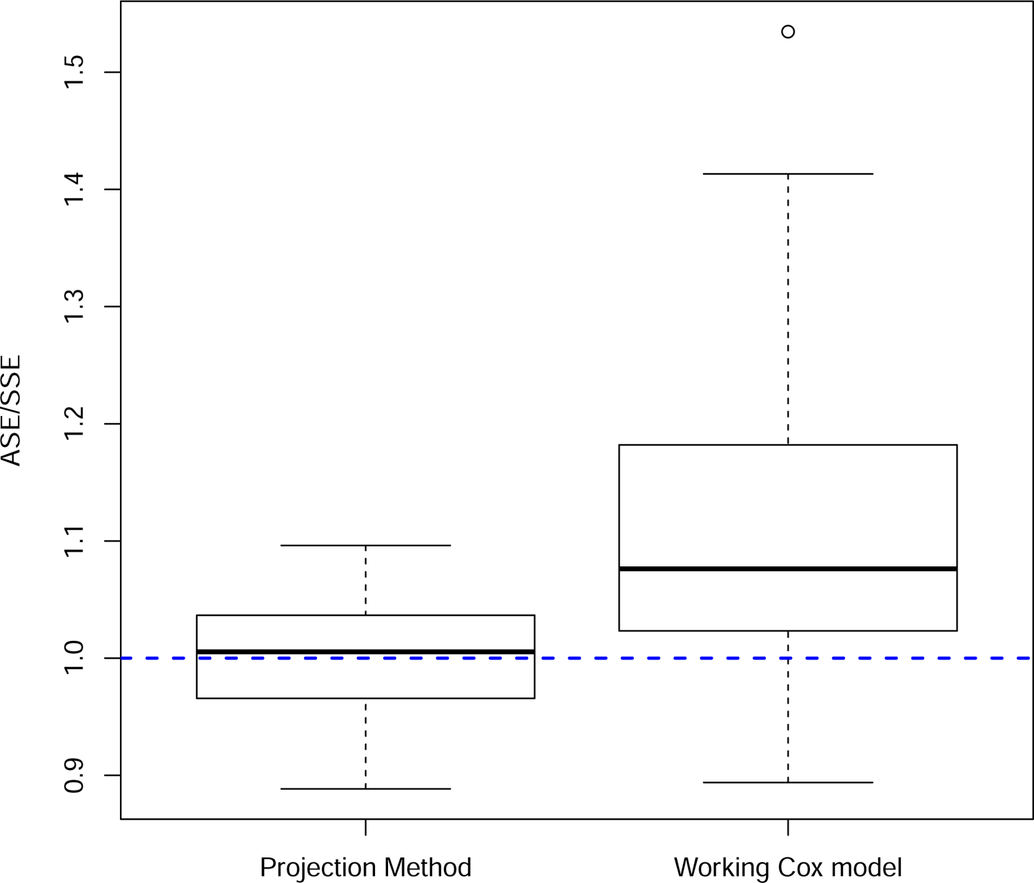
Ratio of the average estimated standard error to the simulation standard error. Results from the 72 parameter combinations specified in Section 3.

3.2. Model misspecification

The robustness of the projection method to model misspecification was examined through simulation. Two types of misspecifications were considered. First, the true survival function was derived from a time-invariant coefficient (proportional hazards) model, which represents a special case of (8) with β_1t = β₁ and β_2t = β₂. For the second misspecification, the Weibull shape parameter was a function of the covariates (−0.2x₁x₂ν) and the survival function

$$S_t\left(\mathit{x},z\right)=\exp \left\{-\exp \left[{\alpha }_t\left(x_1,x_2\right)+{\beta }_{1t}{x}_1+{\beta }_{2t}{x}_2+\gamma z\right]\right\}$$

no longer had the form of a time-varying Cox model, as the covariates were not an additive function of the log negative log survival function. In each case, the projection method based on the time-varying coefficient Cox model (8) was used to estimate the square root expected difference in Brier scores. The simulation framework was the same as described in Section 3.1.

A summary of the results are depicted in Supplemental Figures S1 through S3, with the individual results provided in Supplemental Tables 3 and 4. When the true survival function is generated from the proportional hazards model, the estimated relative bias (mean = 0.032, std dev = 0.106), the ratio of the estimated standard error to simulation standard error (mean = 1.010, std dev = 0.038), and the coverage probability from the 95% confidence interval (mean = 0.941, std dev = 0.022) were good and comparable to the results in Section 3.1. For the case when the Weibull shape parameter was a function of (x₁, x₂) and so the additive time-varying Cox model (8) is inappropriate, there was a drop off in the accuracy of the method. The estimated relative bias remained low, but with greater variability across simulations (mean = −0.002, std dev = 0.153). The estimated standard error was accurate relative to the simulation standard error (mean = 0.989, std dev = 0.050). However, there was poorer coverage in the estimated 95% confidence interval (mean = 0.926).

4. Metastatic Prostate Cancer Example

Metastatic prostate cancer is a lethal disease and the development of a risk model can be helpful for patient counseling, treatment decision making, clinical trial eligibility, and stratification within a clinical trial. The effectiveness of its implementation is a function of the predictive accuracy of the model. In this analysis, a proportional hazards model was developed to explore whether the addition of two new biomarkers, circulating tumor cells (CTC) and serum testosterone, provided added value to the existing biomarkers which are widely used for prognosis. These include prostate specific antigen (PSA), lactate dehydrogenase, presence of visceral disease, and ECOG status. The data were derived from an international randomized clinical trial conducted for metastatic prostate cancer patients previously untreated with chemotherapy. The biomarker analysis did not stratify by treatment, as the survival rates were comparable between the randomized treatments (Saad et al. 2015).

A proportional hazards model was fit to the data and the results are summarized in Table 3. All of the biomarkers were strongly prognostic, however, there were 520 events among the 1303 patients with baseline biomarker data, diminishing the significance of the individual point null tests of association in Table 3. Cumulative martingale residual plots and functional form covariate plots were generated to demonstrate the appropriateness of the proportional hazards model with a loglinear covariate specification. These graphs are provided as Supplemental Figures 4 and 5. The p-values used to test the proportional hazards assumption were generated from the score processes of martingale residuals (Lin et al. 1993; Martinussen and Scheike 2006). A summary of the nested proportional hazards model without the new biomarkers CTC and testosterone is presented in Table 4. Although the remaining biomarkers in the submodel maintain their strong association, the martingale residual plot for ECOG status raises doubt concerning the proportional hazards interpretation (Supplemental Figure 6), signaling the non-nesting of these proportional hazards models.

Using the projection method, Figure 5 depicts the estimated improvement in the expected Brier score, for 1 month to 36 months from the start of treatment, due to the addition of CTC and serum testosterone to the risk model. With a 0.10 threshold, the data indicates an improvement in the Brier score evaluated after 12 months, accounting for the variability in the estimate. It is noted that the survival estimates within 12 months are high (Saad et al. 2015) and thus it is unsurprising that a notable change in calibration does not occur prior to this time point. In contrast, although the point null tests of no association were rejected for all biomarkers, Figure 5 indicates that PSA, the most widely used biomarker for clinical decision making in this population, provides minimal added benefit to a model that includes CTC, testosterone, lactate dehydrogenase, presence of visceral disease, and ECOG status. This indicates that focus on PSA in the metastatic population, to the exclusion of other biomarkers, can lead to suboptimal decision making.

FIGURE 5.

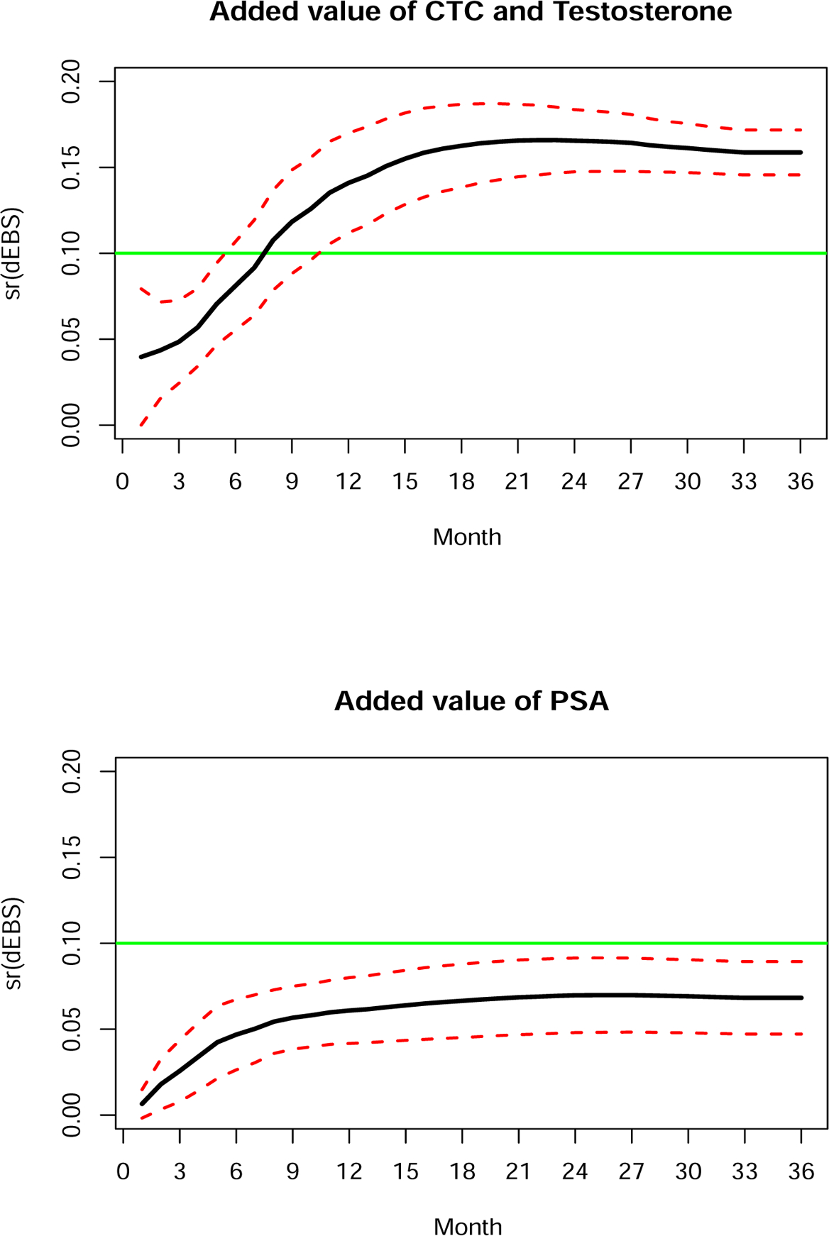
Square root estimated difference in the expected Brier scores [D_n(t)] with 95% confidence bands.

5. Discussion

In practice, new risk factors associated with survival may be costly or invasive to obtain, or may create an overly complex risk score making its implementation less likely by practicing clinicians. A key question, therefore, is whether new factors sufficiently improve the predictive accuracy of the model to warrant inclusion in an updated risk model. In this paper, a method has been developed to evaluate the decrement in the expected Brier score due to the inclusion of new risk factors in a Cox model with possibly time-varying coefficients. Specifically, methodology was developed to accurately estimate the difference in expected Brier scores and to compute an accompanying variance and confidence interval estimate. An important component of the proposed methodology is the recognition of non-nesting in Cox models. Without this adaptation, the application of an incorrectly specified subset risk model inflates the importance of the new factors. Implicit in this work is the recognition that the analyst has carefully developed a model that includes all factors.

A counterargument to this proposal is to simply accept a larger difference in the expected Brier scores due to misspecification of the nested subset model. This choice, however, confounds the decision process on the added value of new factors. Under model misspecification, the difference in the expected Brier scores may be decomposed into ∆(t) + E[π_t(X) − R_t(X)]². Ideally, the decision process should stem soley from ∆(t), with E[π_t(X) − R_t(X)]² resulting from the limitations of the analysis, and not the importance of the new factors under study.

The proposed methodology is based on the premise that the model with all factors is well-calibrated, which requires model diagnostic evaluation. Importantly, if the new factors included are all uninformative, creating a miscalibrated model, the asymptotic normality of $\widehat{\Delta }(t)$ is unlikely to hold (Heller et al. 2017). One approach to guard against this type of miscalibration is to initially perform tests of association to determine the informative new factors to be included in the full model (Pepe et al. 2013).

The projection method can be applied to estimate the difference in expected Brier scores derived from partially nested conditional survival functions

$$E{\left[{\pi }_t\left(\mathit{X},\mathit{Z}\right)-{\pi }_t\left(\mathit{X},\mathit{U}\right)\right]}^2.$$

Estimation proceeds via a time-varying coefficient Cox model derived from the union of factors ${\widehat{S}}_t\left(\mathit{x}.\mathit{z},\mathit{u}\right)$, and the estimated conditional survival functions are obtained through kernel smoothing (6), projecting onto the appropriate subspaces. The estimated change in the expected Brier score follows.

The methodology is sufficiently general to allow weights to be incorporated into the change in the expected Brier score

$$E\left\{w_t\left(\mathit{X},\mathit{Z}\right){\left[{\pi }_t\left(\mathit{X}\right)-S_t\left(\mathit{X},\mathit{Z}\right)\right]}^2\right\},$$

where for example, w_t(X, Z) = [S_t(X, Z) − 0.5]² would give greater weight at the high and low end of the risk scale, offering greater reward for more definitive risk predictions. An alternative weight choice, when the population under study is a low risk or a screening population is w_t(X, Z) = 1 − S_t(X, Z). Selecting this weight would give greater representation to patients that are moved into higher risk with the updated model.

Finally, the evaluation of model improvement can occur in the context of a single data set or within the framework of initial data followed by validation data. In each case, inclusion of the variability for the change in prediction error will increase the level of confidence that the new factors improve prediction error.

Table 1:

Summary of the full proportional hazards model

Biomarker	log(RR)	se[log(RR)]	p-value
sr(PSA)	0.018	0.004	< 0.0001
log(LDH)	0.551	0.135	< 0.0001
Visceral dis	0.322	0.105	0.002
ECOG status	−0.482	0.091	< 0.0001
log(T)	−0.298	0.074	< 0.0001
sr(CTC)×I(CTC ≤ 10)	0.344	0.053	< 0.0001
sr(CTC)×I(CTC > 10)	0.127	0.009	< 0.0001

sr(PSA) = square root prostate specific antigen; log(LDH) = log lactate dehydrogenase; sr(CTC) = square root circulating tumor cells; log(T) = log serum testosterone; RR = relative risk

Table 2:

Summary of the working proportional hazards submodel

Biomarker	log(RR)	se[log(RR)]	p-value
sr(PSA)	0.029	0.003	< 0.0001
log(LDH)	1.239	0.110	< 0.0001
Visceral dis	0.386	0.105	0.0002
ECOG status	−0.508	0.090	< 0.0001

References

- Box GEP and Draper NR (1987). Empirical Model-Building and Response Surfaces. New York: Wiley. [Google Scholar]
- Cai Z and Sun Y (2003). Local linear estimation for time-dependent coefficients in Cox’s regression models. Scandinavian Journal of Statistics, 30, 93–111. [Google Scholar]
- Demler OV, Paynter NP, Cook NR (2015). Tests of calibration and goodness-of-fit in the survival setting. Statistics in Medicine, 34, 1659–1680. [DOI] [PMC free article] [PubMed] [Google Scholar]
- DiCiccio TJ, Monti AC, Young GA (2006). Variance stabilization for a scalar parameter. Journal of the Royal Statistical Society, Series B, 68, 281–303. [Google Scholar]
- Gerds TA and Schumacher M (2007). Efron-type measures of prediction error for survival analysis. Biometrics, 63, 1283–1287. [DOI] [PubMed] [Google Scholar]
- Gneiting T and Raftery AE (2007). Strictly proper scoring rules, prediction, and estimation. Journal of the American Statistical Association, 102, 359–378. [Google Scholar]
- Graf R, Schmoor C, Sauerbrei W, Schumacher M (1999). Assessment and comparison of prognostic classification schemes for survival data. Statistics in Medicine, 18, 2529–2545. [DOI] [PubMed] [Google Scholar]
- Grambsch P and Therneau T (1994). Proportional hazards tests and diagnostics based on weighted residuals. Biometrika, 81, 515–526. [Google Scholar]
- Hall P and Marron JS (1990). On variance estimation in nonparametric regression. Biometrika, 77, 415–419. [Google Scholar]
- Heller G, Seshan V, Moskowitz CS, Gönen M (2017). Inferential Methods to Assess the Difference in the Area Under the Curve From Nested Binary Regression Models. Biostatistics, 18, 260–274 [DOI] [PMC free article] [PubMed] [Google Scholar]
- Horowitz JL (1998). Semiparametric Methods in Econometrics. New York: Springer. [Google Scholar]
- Hougaard P (1986). Survival models for heterogeneous populations derived from stable distributions. Biometrika, 73, 387–396. [Google Scholar]
- Korn EL and Simon R (1990). Measures of explained variation for survival data. Statistics in Medicine, 9, 487–503. [DOI] [PubMed] [Google Scholar]
- Kosorok MR, Lee BL, and Fine JP (2004). Robust inference for univariate proportional hazards models frailty regression models. The Annals of Statistics, 32, 1448–1491. [Google Scholar]
- Lawless JF and Yuan Y (2010). Estimation of prediction error for survival models. Statistics in Medicine, 29, 262–274. [DOI] [PubMed] [Google Scholar]
- Lin DY, Wei LJ, Ying Z (1993). Checking the Cox Model with Cumulative Sums of Martingale-Based Residuals. Biometrika, 80, 557–572. [Google Scholar]
- Martinussen T and Scheike T (2006). Dynamic Regression Models for Survival Data. New York: Springer. [Google Scholar]
- Nam J, Kim J, and Lee S (2005). Equivalence of two treatments and sample size determination under exponential survival model with censoring. Computational Statistics and Data Analysis, 49, 217–226. [Google Scholar]
- Peng L and Huang Y (2007). Survival analysis with temporal covariate effects. Biometrika, 94, 719–733. [Google Scholar]
- Pepe MS, Kerr KF, Longton G, Wang Z (2013). Testing for improvement in prediction model performance. Statistics in Medicine, 32, 1467–1482. [DOI] [PMC free article] [PubMed] [Google Scholar]
- Rosthoj S and Keiding N (2004). Individual survival time prediction using statistical models. Lifetime Data Analysis, 10, 461–472. [DOI] [PubMed] [Google Scholar]
- Saad F Fizazi K, Jinga V, Efstathiou E, Fong PC, Hart LL, et al. (2015). Orteronel plus prednisone in patients with chemotherapy naive metastatic castration-resistant prostate cancer (ELM-PC 4): a double-blind, multicentre, phase 3, randomised, placebo-controlled trial. Lancet Oncology, 16, 338–348. [DOI] [PubMed] [Google Scholar]
- Schemper M (1990). The explained variation in proportional hazards regression. Biometrika, 77, 216–218. [Google Scholar]
- Tian L, Zucker D, and Wei LJ (2005). On the Cox model with time-varying regression coefficients. Journal of the American Statistical Association, 100, 172–183. [Google Scholar]
- Tian L, Cai T, Goetghebeur E, and Wei LJ (2007). Model evaluation based on the sampling distribution of estimated absolute prediction error. Biometrika, 94, 297–311. [Google Scholar]
- Uno H, Cai T, Tian L, and Wei LJ (2007). Evaluating prediction rules for t-year survivors with censored regression models. Journal of the American Statistical Association, 102, 527–537. [Google Scholar]
- Wellek S (1993). A log-rank test for equivalence of two survivor functions. Biometrics, 49, 877–881. [PubMed] [Google Scholar]
Associated Data
This section collects any data citations, data availability statements, or supplementary materials included in this article.