Subcircuits of deep and superficial CA1 place cells support efficient spatial coding across heterogeneous environments

Summary

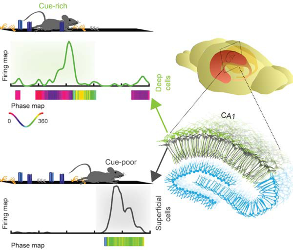
The hippocampus is thought to guide navigation by forming a cognitive map of space. Different environments differ in geometry and availability of cues that can be used for navigation. Although several spatial coding mechanisms are known to coexist in the hippocampus how are they influenced by various environmental features is not well understood. To address this issue, we examined the spatial coding characteristics of hippocampal neurons in mice and rats navigating in different environments. We found that CA1 place cells located in the superficial sublayer were more active in cue-poor environments, and preferentially used a firing rate code driven by intra-hippocampal inputs. In contrast, place cells located in the deep sublayer were more active in cue-rich environments and used a phase code driven by entorhinal inputs. Switching between these two spatial coding modes was supported by the interaction between excitatory gamma inputs and local inhibition.

Graphical Abstract

eTOC Blurb:

Sharif et al., demonstrated the existence of segregated hippocampal circuits for spatial coding across heterogeneous environments. Deep and superficial CA1 place cells used different codes for space depending on the availability of cues. A rapid switch between these two spatial coding modes was supported by the interaction between gamma inputs.

INTRODUCTION

Animals navigate different environments in search of food and shelter, or to escape threats. To successfully accomplish these tasks, they must be able to orient themselves using environmental landmarks or via path-integration. The hippocampal formation is believed to support this process by creating a ‘cognitive map’ of the explored environment (O’Keefe and Nadel, 1978). Hippocampal pyramidal cells that fire selectively when the animal is at a particular location, known as ‘place cells’ (O’Keefe and Dostrovsky, 1971), are considered the building blocks of this cognitive map. Different place cells fire at distinct locations (i.e., in their ‘place fields’) such that the whole environment is represented by the collective activity of the place cell population (O’Keefe, 1976). The correlation of the firing rate of a place cell with animal position is referred as the ‘rate code’ since it is possible for an external observer (and also for a downstream ‘reader’ structure) to accurately decode the animal’s position from the firing rates of the place cell population (Wilson and McNaughton, 1993). In addition, the firing patterns of hippocampal place cells are globally coordinated by theta oscillations, which synchronize place cells with overlapping place fields into functional ‘assemblies’ and represent animal trajectory linking assembly sequences that encode previous, current and future positions (i.e., in ‘theta sequences’; Skaggs et al., 1996; Dragoi and Buzsaki, 2006; Foster and Wilson, 2007; Gupta et al., 2012). Because the spike timing of individual place cells advances with respect to the ongoing theta rhythm as an animal moves through the neuron’s place field (‘phase precession’; O’Keefe and Recce 1993), the animal position can also be decoded from spike theta phase (a ‘phase code’).

It is not clear how the complementary rate code and phase code are used interchangeably to encode animal position (Harris et al., 2002; Mehta et al., 2002; Huxter et al., 2003; Huxter et al., 2008; O’Keefe and Burgess, 2005; Cei et al., 2014; Lasztoczi and Klausberger, 2016; Fernandez-Ruiz et al., 2017). An advantage of the phase code is that it has higher spatial resolution than the rate code (Jensen and Lisman, 2000; Huxter et al., 2008; Tingley and Buzsaki, 2018). On a coarse spatial scale (i.e. tens of cm to meters), larger than the average place field size, a rate code is reliable since place cell firing outside its fields is minimal. However, since the firing rate of a place cell increases and decreases as the animal crosses the field, identical firing rates can correspond to positions separated by up to tens of cm. On the other hand, the spike theta phase of a place cell shows a unidirectional advancement throughout the spatial range of the place field, offering a reliable mechanism to encode position at a fine spatial scale.

A limitation shared by most previous studies is that hippocampal spatial coding was typically investigated in cue-impoverished environments (such as linear tracks or open fields) that potentially reduced the need for fine spatial scale encoding mechanisms. Studies that assessed the modulation of hippocampal place cells by sensory cues, objects and landmarks, reported heterogeneous responses (Knierim et al., 1998; Save et al., 2000; Knierim et al., 2002; Battaglia et al., 2004; Burke et al., 2011; Bourboulou et al., 2019). Another limitation is that spatial coding was investigated largely assuming functionally homogenous cell populations within the individual CA regions. Recent studies, however, outlined distinct spatial/non-spatial representations along the septo-temporal, transverse and radial axes of the hippocampus (Royer et al., 2010; Igarashi et al., 2014; Danielson et al., 2016; Geiller et al., 2017). In the CA1 region in particular, two populations of pyramidal cells have been distinguished based on their position along the radial axis (Lorente de No, 1934; Slomianka et al., 2011). Pyramidal cells located closer to the stratum oriens (or ‘deep’ sublayer) show striking differences with pyramidal cells located closer to the stratum radiatum (‘superficial’ sublayer) in terms of anatomy, physiology and gene expression (Mizuseki et al., 2011; Lee et al., 2014; Maroso et al., 2016; Valero et al., 2015; Oliva et al., 2016a; Cembroski et al., 2016). We hypothesize that this heterogeneity among CA1 pyramidal cells confers the hippocampus a larger computational flexibility that could support spatial coding across different environments.

Based on this background, we hypothesized that the availability of cues in the environment affects the properties of the hippocampal spatial map. In cue-impoverished environments a low-resolution map, supported by the rate code is generated, whereas in cue-rich environments, where space is fragmented by prominent local cues, a finer resolution, phase-coding dominated map, becomes dominant. To test this hypothesis, we recorded hippocampal place cells in mice and rats that navigated sequentially in cue-poor and cue-rich environments. We found that superficial and deep CA1 place cells were mainly recruited in cue-poor and cue-rich environments, respectively. In cue-poor environments, the rate code dominated as place cells were more spatially selective and cell firing rates carried more spatial information than cells’ spike theta phases. In cue-rich environments, the phase code dominated as the spatial information carried by firing rates was decreased and cells’ spike theta phase precession became stronger. This shift between rate and phase codes was regulated by a differential control of CA1 place cells by CA3 or entorhinal inputs, gated by local interneurons. These findings suggest that environmental features influence the anatomical and computational substrate of hippocampal representation of space.

RESULTS

Superficial and deep CA1 place cells map cue-poor and cue-rich environments, respectively

Dissecting the mechanisms governing place cells in freely moving animals is complicated due to the large number of uncontrolled variables such as head direction, physical interaction with objects, and mixed contribution of distal and local cues (Knierim et al., 1998; Huxter et al., 2008; Ravassard et al., 2013; Jayakumar et al., 2019). To avoid such confounding factors, we tested head-fixed mice (n = 6) running on a non-motorized treadmill to collect water rewards (Figure S1). The treadmill had a 230-cm belt with two zones, one deprived of local cue (‘cue-poor’ zone) and the other enriched with several large tactile cues (‘cue-rich’ zone). The influence of distal visual cues was minimized by the presence of black panels on each side of the track. This task presents the advantage that the same cell population is monitored across both types of environments on each trial. We used high-density silicon probe electrodes to monitor the unit activity and local field potentials (LFPs) from the hippocampal CA1 region.

CA1 pyramidal neurons displayed place fields that tiled the whole treadmill belt and that were stable throughout the recording session (Figure 1A and Figure S1). Mice ran with similar speeds in both zones (Figure S1, p > 0.05). We divided place cells into two groups based on whether the location of place fields’ peak firing rate was within the cue-rich (n = 325) or cue-poor (n = 120) zones. The density of place fields (0.053 ± 0.009 /0.044 ± 0.006 fields/cm in n = 34 sessions; Figure 1A) was similar for the two groups (p > 0.05, Kruskal-Wallis test) but place field width was, on average, smaller for cells encoding the cue-rich zone (Figure 1B; p = 1.17e-4). Next, we examined the anatomical distribution of cells along the CA1 radial axis. We defined the middle of the CA1 pyramidal layer as the recording site where sharp-wave ripples had the largest amplitude (Figure 1C; Mizuseki et al., 2011; Oliva et al., 2016b). A majority of the cells encoding the cue-rich zone were located above this point (i.e. in the deep sublayer), while cells encoding the cue-poor zone were preferentially located below the middle of the layer (i.e. in the superficial sublayer; Figure 1D–E; p = 2.9e-8). Of the total sample of place cells across all animals, 74 % of all the place cells with place fields in the cue-rich zone were deep pyramidal cells while 72% of place cells with place fields in the cue-poor zone were superficial pyramidal cells (Figure 1F). These results show that cue-rich and cue-poor environments are differentially represented by anatomically segregated populations of hippocampal place cells.

Figure 1: Segregated CA1 subpopulations for navigation in different environments.

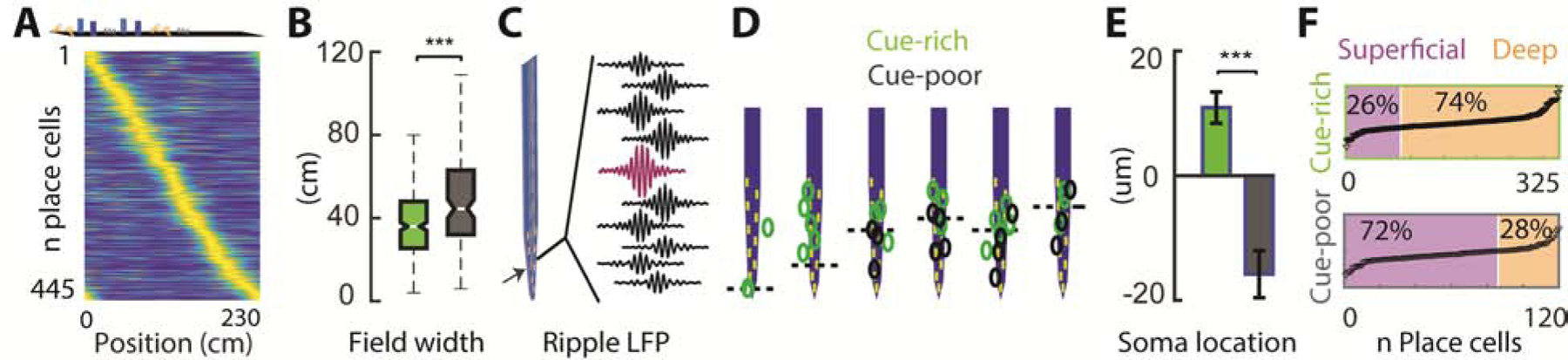
A) Plot showing color-coded place fields of CA1 pyramidal cells on the belt (n = 445). Cells were sorted according to the location of their highest firing rate and rates were normalized to this maximum value. Top: illustration of object distribution on the belt. B) Place fields in the cue-poor zone were wider than those in the cue-rich zone (n = 120/325 cells from 6 mice, p = 1.17e-4, Kruskal-Wallis test). C) Example filtered LFP traces (120–250 Hz) showing largest ripple amplitude in the middle of the CA1 pyramidal layer (magenta). D) Soma location of place cells encoding the cue-poor (grey) and cue-rich (green) zones, relative to the middle of the pyramidal layer (dashed line), in an animal example. E) Average soma location relative to the middle of the pyramidal layer for all place cells (p = 2.9e-8, mean ± s.e.m.). F) Fraction of deep and superficial CA1 place cells encoding the cue-rich and cue-poor zones (p = 9e-11, Fisher’s exact test). Neurons (black triangles) were sorted according to their distance to the middle of the pyramidal layer.

Different spatial codes in cue-poor and cue-rich environments

Next, we asked whether spatial encoding of the two zones of the belt were supported by similar or distinct coding schemes. To investigate the place coding influence of local cues on neurons as a function of their anatomical location, we divided the CA1 place cell population into four groups: cue-rich deep (n = 241), cue-rich superficial (n = 84), cue-poor deep (n = 34) and cue-poor superficial (n = 86).

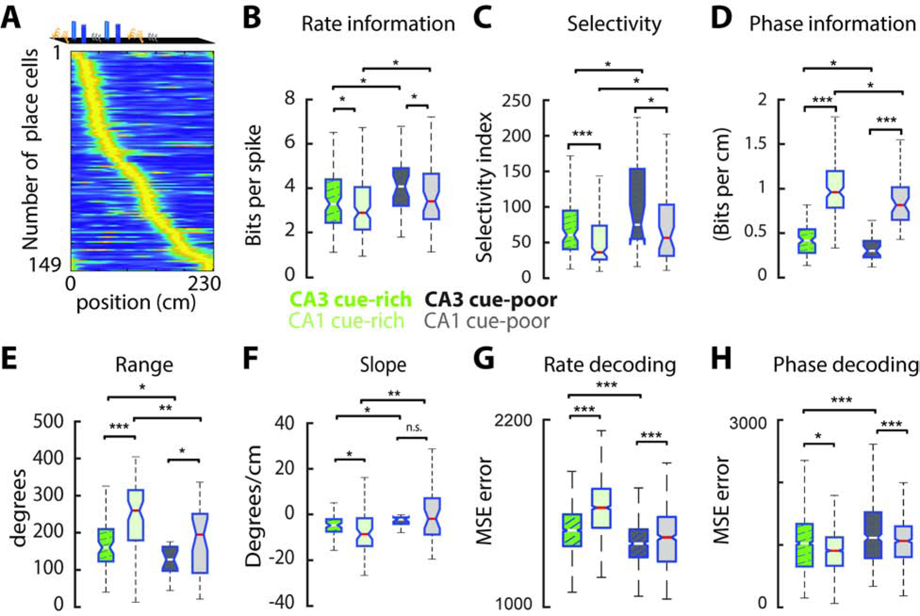
Spatial information encoded in firing rate of place cells differed across belt zones and CA1 sublayers. Firing rates of place cells in the cue-poor zone carried more spatial information than those in the cue-rich zone (Figure 2A,B; F_(1,444) = 61.09, p= 0 main effect of belt zone, 2-way ANOVA). Within each zone of the belt, superficial place cell firing rates were more informative than those of deep place cells (Figure 2A,B; F_(1,444) = 17.8, p= 0 main effect of layer, 2-way ANOVA, with no significant effect of factor interaction). This effect was explained by lower out-of-field firing activity within both the cue-poor zone and the superficial sublayer (Figure 2C, F_(1,444) = 33.6/ 8.11, p=0.0046/ 0 main effect of belt zone and layer respectively, with no significant effect of factor interaction). We found similar differences across belt zones and anatomical sublayers for other place cell metrics as well (Figure S2), suggesting a less efficient firing rate code in the cue-rich zone and in the deep CA1 place cell subpopulation.

Figure 2: Spatial coding properties differ in the cue-rich and cue-poor zones of the belt.

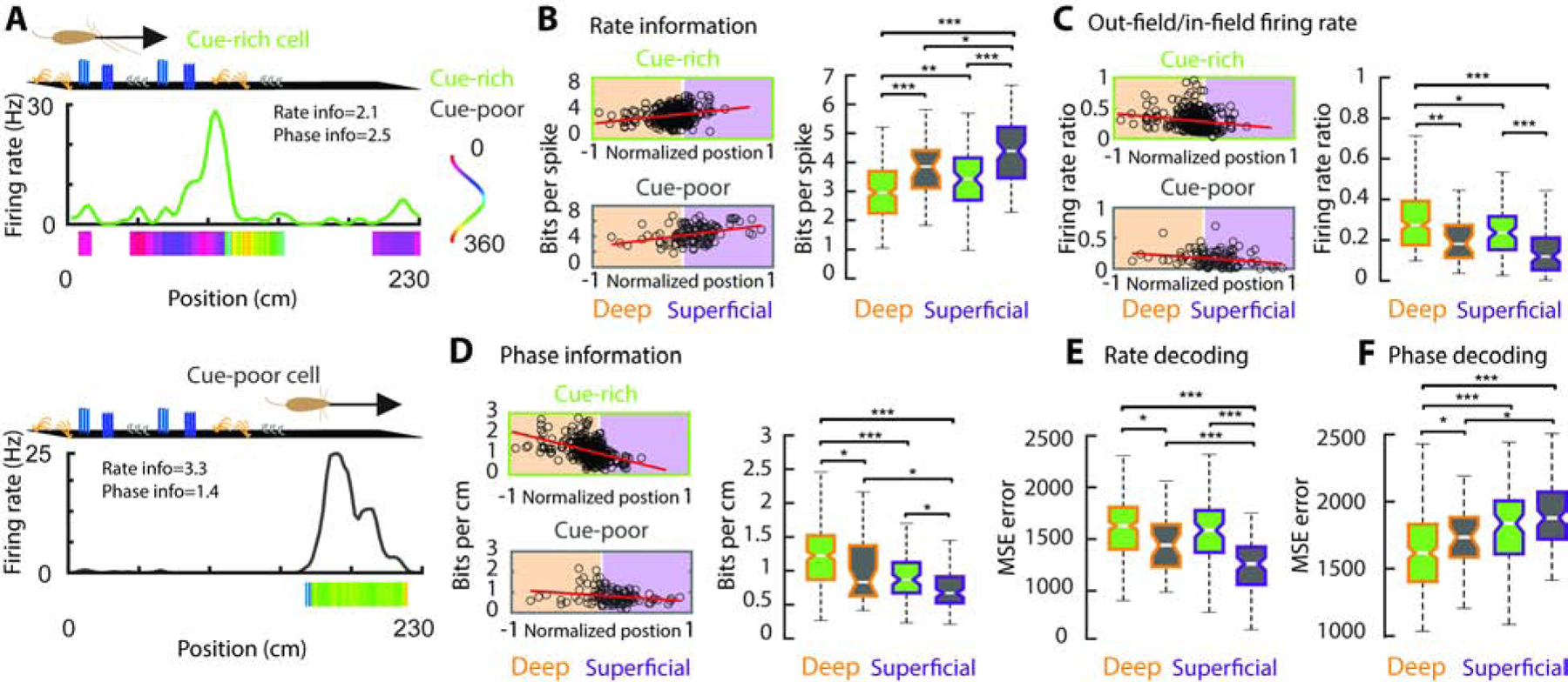
A) Firing rate and spike-phase maps for single place cell examples in the cue-rich (top) and cue-poor (bottom) zones of the belt. Solid line, average firing rate per spatial bin across trials. Color bar, average spike theta-phases per bin (bins with no spikes or distribution of spike-phases with p>0.01, Rayleigh test, are in white. Top arrow, running direction. B) Left panels: spatial information encoded in the firing rates, as a function of cell location along CA1 radial axis (normalized position), for place cells in the cue-rich and cue-poor zones of the belt. Black circles are individual cells; white line, middle of the pyramidal layer; red line, correlation between spatial information and cell location. Right panels: population distribution. C) out-of-field / in-field firing rate ratio. D) Spatial information encoded in the spike theta-phases of place cells. E) Spatial decoding accuracy with firing rates and spike theta-phases (F) */**/*** P < 0.05/ 0.01/ 0.001, Tucker’s post-hoc test.

Next, we examined the spatial information carried by cells’ spike theta phases. For this, we implemented spike theta-phase maps by computing the circular average of instantaneous spike theta-phases in each belt position (Methods). These maps revealed stereotyped phase patterns inside the place fields (Figure 2A and Figure S2). As opposed to firing rates, place cells’ spike theta phases carried more spatial information in the cue-rich zone relative to the cue-poor zone (Figure 2D; F_(1,444) = 17.09, p= 0, effect of belt zone, 2-way ANOVA). Further, spike phases of deep layer neurons were more spatially informative (Figure 2D; F_(1,444) = 33.01, p= 0 effect of layer, 2-way ANOVA, with no effect of interaction). These differences across CA1 sublayers and belt zones were consistent across animals and could not be explained by any single animal contribution (Table S1).

To further compare how animal position was encoded by firing rates and spike theta phases, we used 70% of the trials to train a maximum correlation coefficient classifier to predict animal position from either the firing rate maps or the spike theta phase maps and then tested the classifier decoding accuracy on the remaining 30% of the trials (Figure S3). While position decoding accuracy was high for both firing rate and spike theta phase (Figure 2E–F; p < 1e-67 for all cases when compared to randomly shuffled data; Kruskal-Wallis test), position decoding errors were significantly smaller in the cue-poor zone relative to the cue-rich zone for firing rates (Figure 2E; p = 3.0e-88, Kruskal-Wallis test) and were significantly smaller in the cue-rich zone relative to the cue-poor zone for spike theta phases (Figure 2F; p = 1.7e-15). These results further support that position information is more accurately conveyed by the rate code in cue impoverished environments and by the spike theta phase code in cue-rich environments.

To analyze the potential effect of running speed in different parts of the belt on spatial coding properties, we divided all trials into three blocks of different speed and calculated place fields independently for each of them. The reported differences in spatial coding between the cue-rich and cue-poor zones were maintained regardless of running speed (Figure S4). To evaluate the potential effect of the reward, we performed additional control experiments in which the reward location was changed and compared place field and spatial coding metrics between cue-rich and cue-poor zones. We found the same relationships (Figure S4), indicating that the observed differences in place cell properties were a consequence of the presence or absence of local cues on the belt rather than the location of the reward.

Theta phase precession and temporal compression of space by theta sequences

Place cells display a monotonic advance of their firing relative to the ongoing theta rhythm as the animal transverse the place field of the neuron, resulting in a systematic shift forward in successive theta cycles (‘phase-precession’; O’Keefe and Recce, 1993). We hypothesized that differences in cell theta phase precession accounted for differences in position decoding accuracy using spike theta phase maps. We thus examined the phase precession of deep and superficial CA1 place cells in the cue-rich and cue-poor zones of the belt (Figure 3 and Figure S2). We restricted this analysis to place fields with significant phase-position correlation (n = 305 place fields from 6 mice; p < 0.05, linear-circular regression).

Figure 3: Wider phase precession in the cue-rich zone of the treadmill.

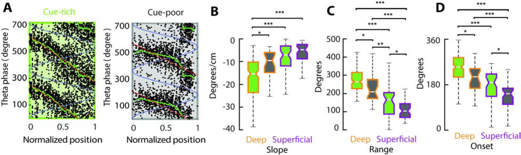
A) Spike theta-phase versus normalized position inside the place field for two example place cells in the cue-rich (left) and cue-poor zones (right). Each black dot is one spike. Red line show phase-position correlation and green line mean theta phase. Two theta cycles (blue line) are shown for clarity. B) Phase precession slopes for cue-rich (n = 178/ 54 deep/ superficial place cells, respectively) and cue-poor place cells (n = 26/ 47 deep/ superficial place cells, respectively). C) Theta phase-range of place cell spikes. D) Spike theta-phases at the onset of the place field. */** P < 0.05/ 0.01/0.001, Tucker’s post-hoc test.

Place cells displayed a steeper phase-precession slope (Figure 3A–B; F_(1,304) = 6.45, p= 0.011 main effect of belt zone, 2-way ANOVA) and a wider range of spike theta phases in the cue-rich zone compared to the cue-poor zone (Figure 3C; F_(1,304) = 17.08, p= 0, with no significant effect of factor interaction). Deep place cells also had steeper slopes and wider phase ranges than superficial place cells (F_(1,304) = 8.39/ 98.3, p = 0.004/ 0 main effect of layer for slope and range respectively, with no effect of interaction). These differences were partly explained by an initially higher spike theta phase (closer to theta peaks or 360°), upon place field onset, for cue-rich zone place cells and in those located in the deep sublayer (Figure 3A,D; F_(1,304) = 17.24/ 63.97, p = 0/0 effect of belt zone and layer, with no effect of interaction). Such wider and steeper theta-phase precession might explain the higher phase-based spatial information and decoding accuracy of cue-rich zone and deep CA1 cells.

Our results from single cell spatial coding properties suggested that theta phase representation of space is more pronounced in the cue-rich zone than in the cue-poor zone. We thus hypothesized that such single neuron differences should be reflected at the level of hippocampal cell assemblies.

As an animal runs across an environment, different place cell assemblies activate in a sequential manner along the animal trajectory. At any given location, the place fields encoding current positions overlap with the tails of place fields encoding previous and upcoming adjacent locations (Figure 4A). Place cells encoding previous positions discharge earlier in the theta cycle, followed by place cells encoding current and future positions (Figure 4A). These “theta sequences” constitute temporally compressed ensemble representations of spatial trajectories (Skaggs et al., 1996; Dragoi and Buzsaki, 2006; Foster and Wilson, 2007). The degree of ‘temporal compression’ of space can be estimated as the ratio between the distance of two neighboring place fields peaks and the time lag between the spikes of the two corresponding place cells within one theta cycle (Figure 4B; Dragoi and Buzsaki, 2006).

Figure 4: Environmental cues affect temporal compression of space by hippocampal theta sequences.

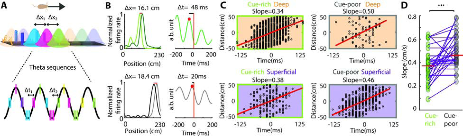
A) Overlapping place fields along animal’s trajectory (top). ∆x₁ and ∆x₂, distance between the peaks of successive fields. Firing of example place cells (color of cell’s spikes match that of their place field) in successive theta cycles. ∆t₁ and ∆t₂, time lag between the firing of two place cells in the same theta cycle. B) Example of two overlapping place fields (left) and theta-scale cross-correlation of their spikes (right) for a pair of cue-rich (top) and cue-poor zone (bottom) place cells. ∆x, distance between place field peaks; ∆t, time lag between the two cell spikes in the first theta cycle (red dot). C) Correlation between place field peak distance (∆x) and theta time lag of their spikes (∆t) for all overlapping CA1 place fields from deep and superficial place cells in the cue-rich (left ; n = 1759/ 236 pairs) and cue-poor (right; n = 80/ 614) zones. Each black circle is one cell pair. Red line indicates correlation slope (∆x/∆t). D) Compression slopes calculated in C) are displayed in the same axes for comparison purposes. D) Session by session comparison of compression slopes in the cue-rich versus the cue-poor zones (n = 34 sessions from 6 mice; p < 0.001, t-test).

To examine differences in hippocampal theta sequences, we calculated the correlation between place field peak distances and theta-scale time lags (spatial compression) measured from overlapping place field pairs, considering separately the cue-rich and cue-poor zones of the belt and the deep and superficial CA1 sublayers (Figure 4C). The slope of this correlation was significantly higher in the cue-poor zone than in the cue-rich zone but did not significantly differ across CA1 sublayers (Figure 4C–D, F(1,532) = 6.13/ 2.22, p = 0.013/ 0.14, 2-way ANOVA for belt zone and layer respectively, with no effect of factor interaction). Theta compression slopes were also higher in the cue-poor than in the cue-rich zone when individual sessions were compared (p < 0.001, t-test, n = 34 sessions). These results indicate a more compressed ensemble representation of space in the cue-poor zone compared to the cue-rich zone. We found no differences in theta frequency, theta power or running speed between cue-rich and cue-poor zones (Figure S1 and S5; p > 0.05, Kruskal-Wallis test). Furthermore, these results were maintained when the reward location on the belt was changed (Figure S4) or when trials of different speed were segregated and the analysis repeated independently for each speed block (Figure S4).

CA3 pyramidal cells have similar spatial coding properties to superficial CA1 cell

We found that superficial and deep CA1 cells expressed place fields preferentially in the cue-poor and cue-rich zones of the belt and optimally convey spatial information via rate code and phase code, respectively. Because the CA3 input is the main driver of CA1 place cell firing (Csicvari et al., 2003; Dragoi et al., 2006; Nakashiba et al., 2008; Davoudi and Foster, 2019) and because CA3 input is more effective at driving superficial CA1 pyramidal cells (Valero et al., 2015; Masurkar et al., 2017), we next investigated the spatial coding properties of CA3 neurons.

CA3 place fields were expressed in both zones of the belt (Figure 5A and Figure S6; n = 40/ 109 place cells in the cue-rich and cue poor zones with a density of 0.073/0.063 fields/cm respectively, from 6 mice). CA3 place cells displayed similar differences in spatial coding properties as CA1 place cells: they had better rate coding in the cue-poor zone and better phase coding in the cue-rich (Figure 5B–H), and place fields in the cue-poor zone were wider than those in the cue-rich zone (Figure S6; n = 40/109; p = 0.01, Kruskal-Wallis test). Overall, CA3 cells carried more spatial information in their firing rates than CA1 neurons (Figure 5 B; p = 0.042/ 0.012 for cue-rich and cue-poor zones, Kruskal-Wallis test) and their fields were more spatially selective (Figure 5 C; p = 4.4e-5/ 0.024) and less sparse (Figure S6; p = 0.043/ 0.035). In contrast, spike-theta phase was less spatially informative in CA3 than in CA1 (Figure 5D; p = 5.7e-31/ 0.023) and the range and slope of phase precession were smaller in CA3 than in CA1 (Figure 5 E–F; p = 4.7e-6/0.023 for range and p = 0.018/0.028 for slope), consistent with our previous hypothesis that the low spatial information of spike-theta phases could result from a reduced phase-precession. Finally, we compared the accuracy of position decoding using either firing rates or spikes phases. Relative to CA1 cells, decoding errors for CA3 cells were smaller when firing rates were used (Figure 5G; p = 1.8e-82/ 5.5e-4) but were higher when spike-phases were used (Figure 5H; p = 0.023/ 1.7e-9). In summary, rate coding was more reliable in CA3 than in CA1 and phase coding was more reliable in CA1 than CA3. Consequently, CA3 spatial coding properties were more similar to those of CA1 superficial cells.

Figure 5: CA3 place cells have more precise spatial rate coding and poorer phase coding than CA1.

A) Plot showing firing maps of CA3 pyramidal cells on the belt (n = 109 cue-rich and 40 cue-poor zone cells). Cells were sorted according to the location of their highest firing rate and rate maps normalized to this maximum value. B) CA3 place cells carried more spatial information in their firing rates than CA1 place cells. C) CA3 place fields were more spatially selective than CA1 place fields. D) CA3 place cells carried less spatial information in their spike-phases than CA1 place cells. E) The range and slope (F) of phase-precession were smaller in CA3 than in CA1. G) Relative to CA1 cells, spatial decoding accuracy of CA3 cells was higher when using firing rates but lower when using spike phases (H). Note that, for all metrics shown, the trends between cue-poor and cue-rich zones were similar for CA3 and CA1 place cells. */**/*** P < 0.05/ 0.01/ 0.001, Kruskal-Wallis test.

CA3 and EC gamma inputs preferentially control place cells in cue-rich and cue-poor zones

Together with previous evidences of a stronger drive of superficial CA1 by CA3 inputs (Valero et al., 2015; Masurkar et al., 2017), our results suggest that strong CA3 inputs may contribute to the more efficient rate coding of CA1 cells in the cue-poor zone. On the other hand, inputs from the layer 3 of entorhinal cortex (EC3) were shown to modulate the degree of phase-precession in CA1 (Schlesiger et a., 2015; Fernandez-Ruiz et al., 2017) and may contribute to the wider phase-precession range and improved phase-coding in the cue-rich zone. Therefore, we compared the strength of CA3 and EC3 inputs to CA1 in the two zones of the belt.

We replicated previous results showing that CA3 and EC3 inputs elicit LFP gamma oscillations of different frequency (slow-gamma (30–50 Hz) and mid-gamma (60–100 Hz), respectively) and theta-phase preference in CA1 (Figure 6A–B and Figure S5; Colgin et al., 2009; Schomburg et al., 2014; Lasztoczi and Klausberger, 2016; Fernandez-Ruiz et al., 2017; Lopes-dos Santos et al., 2018). To estimate the respective strength of these two inputs in each zone of the belt, we detected burst events of slow-gamma and mid-gamma oscillations during running (Figure 6C) and compared their power and frequency. The power of CA1 slow-gamma events was the largest in the cue-poor zone (Figure 6D; p < 1.8e-100, Kruskal-Wallis test) while the power of CA1 mid-gamma events was the largest in the cue-rich zone (Figure 6E; p < 2.4e-29), and the ratio of mid-gamma to slow-gamma events was the largest in the cue-rich zone (Figure 6F, p = 1.4e-4, rank-sum test). Slow-gamma power in the CA3 pyramidal layer was stronger in the cue-poor than in the cue-rich zone (Figure 6G; p = 2.1e-5, sign-rank test), mirroring CA1 slow-gamma.

Figure 6: Slow and mid gamma frequency inputs to CA1 place cells dominate in the cue-poor and cue-rich zones, respectively.

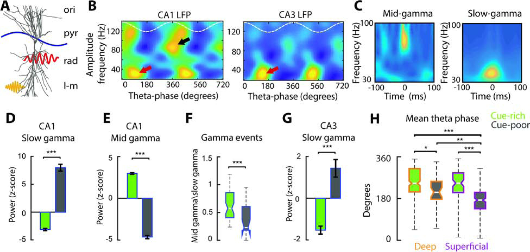
A) Schema summarizing dendritic targets and temporal organization within the theta cycle (blue line) of the two main excitatory inputs to CA1 pyramidal cells: CA3 slow gamma (red) and entorhinal layer 3 (EC3) mid-gamma (yellow) inputs. ori= stratum oriens, pyr= pyramidal layer, rad= stratum radiatum, l-m= striatum lacunosum-moleculare. B) Average theta-phase gamma-amplitude comodulograms from CA1 (left) and CA3 (right) pyramidal layer LFPs (n = 6 mice). Two theta cycles (white dashed line) are shown for clarity. Note the presence of two theta-modulated gamma components in CA1, of slow (red arrow, 30–50Hz) and mid-frequency (black arrow, 60–100 Hz) and distinct theta phase preference, while one component is visible in CA3 (red arrow, 30–40 Hz). C) Wavelet spectrograms of detected mid-gamma (left) and slow-gamma (right) bursts. D) Average power for CA1 slow-gamma events and (E) mid-gamma events in the cue-rich and cue-poor zones (n = 7480 slow gamma events and 4426 mid-gamma events in 6 mice). F) Ratio of mid- and slow-gamma events in the cue-rich and cue-poor zones. G) CA3 slow gamma power was higher in the cue-poor zone, matching CA1 slow gamma distribution. */**/*** P < 0.05/ 0.01/ 0.001, Kruskal-Wallis test. H) Preferred theta phase of firing for deep and superficial cells in the cue-poor and cue-rich zones. */**/*** P < 0.05/ 0.01/ 0.001, Tucker’s post-hoc test.

Since the relative strength of CA3 and EC3 inputs has been shown to modulate the theta-phase preference of CA1 spikes (Mizuseki et al., 2011; Fernandez-Ruiz et al., 2017; Oliva et al., 2016a; Navas-Olive et al., 2020), we hypothesized that CA1 cells encoding the cue-rich zone will preferentially discharge closer to the theta peak, the preferred phase of EC3 input, while CA1 cells encoding the cue-poor zone will preferentially discharge closer to the theta trough, due to stronger CA3 drive. Accordingly, CA1 cells encoding the cue-rich zone (n = 241 deep and 84 superficial cells) discharged closer to the theta peak (360°) than CA1 cells encoding the cue-poor zone (n = 34 deep and 86 superficial cells) (Figure 6H; F(1,444) = 37.4/ 14.78, p = 0/ 1e-4, 2-way ANOVA for belt zone and layer respectively, with no significant effect of factor interaction). These results suggest that CA3 input preferentially drive place cells in the cue-poor zone while entorhinal inputs exert a stronger control over CA1 in the cue-rich zone. This interpretation is in agreement with a stronger entorhinal innervation of deep CA1 pyramidal cells (Masurkar et al., 2017).

Recruitment of local interneurons is modulated by environmental features

Our findings suggest that a shift in the relative strength of CA3 and EC3 inputs drive the shift between the rate code and phase code modes of spatial representation in the cue-poor and cue-rich zones of the belt. Since the strength of interneuron recruitment by CA1 place cells is dynamically modulated by factors such as learning, network synchrony or location within the place field (Dupret et al., 2013; Fernandez-Ruiz et al., 2017; Grienberger et al., 2017; English et al., 2017; McKenzie et al, 2019), we investigated whether the recruitment of local interneurons by CA1 pyramidal cells was modulated as a function of environmental features and could thus contribute to the shift in spatial coding we observed.

We identified putative monosynaptically connected pyramidal – interneuron cell pairs from the presence of a significant short-latency (0.5–3 ms) peak in the cross-correlograms of spike times (Figure 7A and Figure S7; n = 142 pairs in 6 mice; English et al., 2017). Spike-transmission probability was defined as excess in postsynaptic cell firing 0.5–3 ms following presynaptic cell spikes, after correcting for presynaptic firing rate and slower timescale co-modulation (see Methods). Spike-transmission probability was estimated for each zone of the belt by implementing pyramidal cell – interneuron cross-correlograms for spikes from the cue-rich and cue-poor zones separately (Figure 7A). We calculated the change in spike-transmission probability between cue-rich and cue-poor zones ((cue-rich – cue-poor) / (cue-rich + cue-poor)) for each pair. Spike-transmission was higher on average in the cue-rich than in the cue-poor zone (Figure 7B; p = 7.8e-7, sing-rank test), suggesting a differential recruitment of interneuron populations across belt zones. Furthermore, for interneurons that had more than one presynaptic partner (n = 34), the spike-transmission probability of all presynaptic partners tended to follow a common trend, exhibiting highest spike-transmission probability value in the same zone of the belt (Figure 7C–D and Figure S7; p = 8.2e-7, sing-rank test). In other words, if one of the pre-synaptic pyramidal cells had its highest spike-transmission probability in the cue-poor zone, the other pre-synaptic partners were more likely to have their highest spike-transmission probability in the cue-poor zone that is called similarity index here (Figure 7C,D and Figure S7). Spike-transmission probability as estimated here can be influence by changes in postsynaptic excitability (English et al., 2017). We thus compared firing rates across belt zones for interneurons that were preferentially recruited in either the cue-rich or cue-poor zones and found that they were not significantly different (Figure S7). Last, we found that interneurons preferentially recruited in cue-poor and cue-rich zones tended to show distinct electrophysiological properties such as burstiness and recruitment during sharp-wave ripples (Figure S7), suggesting that they might correspond to different types of interneurons differentially recruited by superficial and deep CA1 cells.

Figure 7: Variable recruitment of local inhibition in the cue-rich and cue-poor zones.

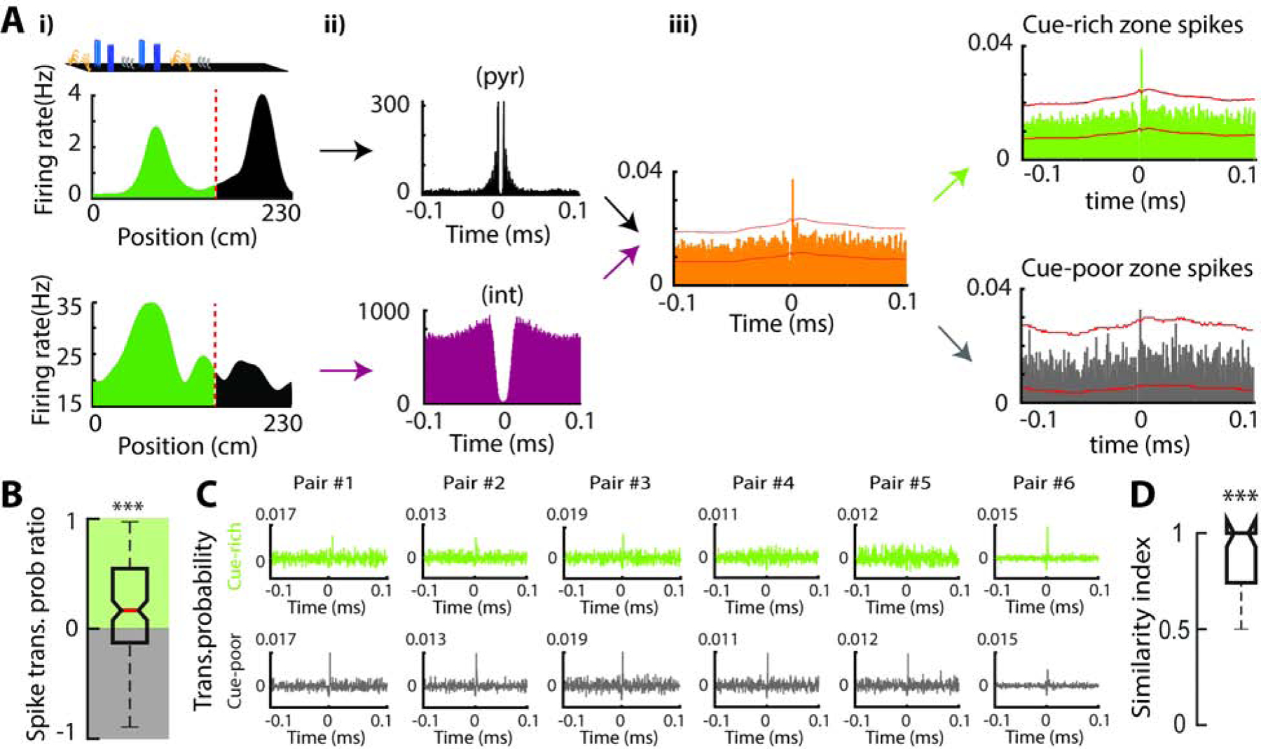
A) Example of a monosynaptically connected CA1 pyramidal cell-interneuron pair. i) Firing maps for the pyramidal cell (top) and interneuron (bottom). The pyramidal cell has one place field in the cue-rich (green area) and another in the cue-poor zone (black). ii) On the left are auto-correlograms for the pyramidal cell (black) and interneuron (red). The spike trains’ cross-correlogram (in orange) display a sharp peak, indicating an enhanced probability for the interneuron to discharge 2 ms after the pyramidal cell. iii) Cross-correlograms constructed only from spikes in the cue-rich (green) or cue-poor zones (gray) showing that the pyramidal cell recruited the interneuron mostly in the cue-rich zone. Note that each cross-correlograms here is normalized to the number of the presynaptic spikes. Red lines indicate significance levels (p < 0.001). B) Change in spike-transmission probability across zones of the belt ((cue_rich– cue_poor) / (cue_rich+ cue_poor)) for all significant pairs (n = 142 from 34 sessions in 6 animals), showing a bias towards cue-rich zones (p < 7.8e-7, sign-rank test). C) Example of an interneuron connected to six pre-synaptic pyramidal cells and receive majority of its excitation from cue-poor zone presynaptic spikes. For each pair, baseline-subtracted cross-correlograms is shown for spikes in the cue-poor (black, top) and cue-rich (green, bottom) zones. Note that in 5 out of the 6 pairs, spike-transmission probability was stronger in the cue-poor zone. Therefore, the pair similarity index for this interneuron is 0.67 indicating that it tends to receive more pre-synaptic excitation from cue-poor zone spikes. D) Similarity index for all interneurons with more than one presynaptic pyramidal cell indicating a strong probability to share the same spatial preference for all the connections (n= 34 interneurons; p < 8.2e-7, sign-rank test).

Overall, these results suggest that distinct population of interneurons are differentially recruited in each zone of the belt and might contribute to the shifts between rate and phase code.

Place cell properties in 2D environments recapitulate the results during head-fixed running

The treadmill apparatus was effective to dissect the influence of local cues on hippocampal spatial coding. Yet, whether the results in head-fixed animals generalize to more natural behaviors and other species is unclear. To address this issue, we recorded CA1 (n = 249) and CA3 (n = 185) place cells in rats (n = 5) as they freely foraged for scattered food rewards in a circular arena that was either empty (‘open maze’) or enriched with 4–6 large objects (‘object maze’; Figure 8A–B). In agreement with the treadmill results, a larger proportion of deep CA1 place cells had place fields in the objects maze than in the open maze (n = 24 sessions; p = 0.02, rank-sum test), while the converse was true for superficial CA1 place cells (n = 24; p = 0.03).

Figure 8: Rate and phase coding properties of place cells in 2D environments.

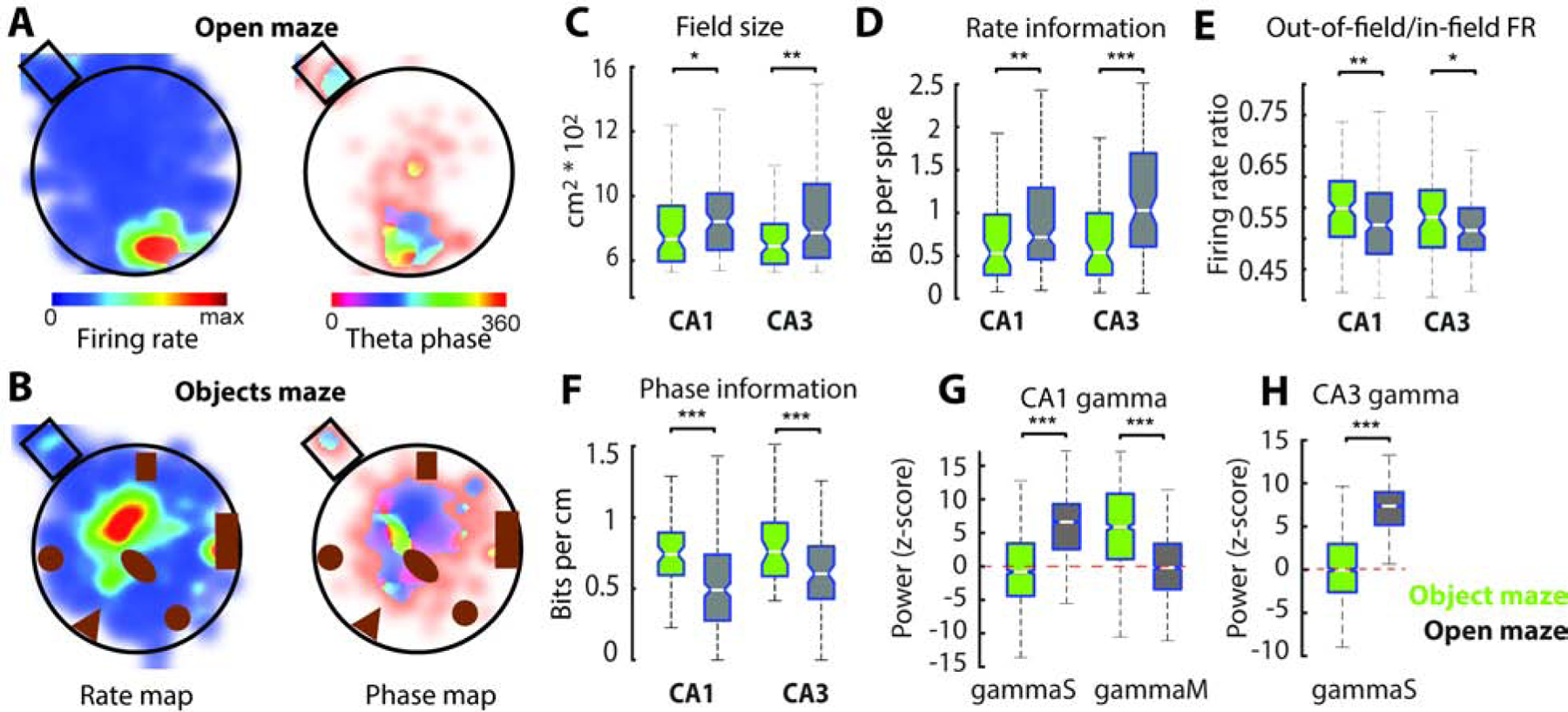
A) Firing rate (left) and spike-phase (right) maps of representative CA1 place cells while a rat was exploring an open empty maze or the same maze with objects (B). C) Place fields were wider in the empty maze (n = 132/ 103 CA1 and CA3 cells from 5 rats) than in the objects maze (n = 117/ 82 cells from 5 rats). D) Spatial information encoded in the firing rates of CA1 and CA3 place cells was higher in the open maze than in the objects maze. E) Place cells fired more spikes outside their place fields in the objects maze than in the open maze. F) Spatial information encoded in the spike-phases of CA1 and CA3 place cells was higher in the objects maze than in the open maze. G) Power of CA1 slow (n = 2563/ 1969 events from 5 rats) and mid gamma (n = 1398/ 1074) bursts in the open and object mazes. H) Power of CA3 slow gamma burst (n = 1936/ 1507 events) in the open and object mazes. */**/*** P < 0.05/ 0.01/ 0.001, rank-sum test.

We calculated spike-rate and spike theta-phase maps in a similar way as before but for two-dimensional space bins. Place fields in the objects maze were smaller than in the empty maze (Figure 8C; p = 0.03/ 0.003 for CA1 and CA3, rank-sum test) but their peak firing rates were not significantly different (Figure S8; p > 0.05). Firing rate of place cells carried more spatial information in the open maze than in the objects maze (Figure 8D; p = 5.6e-3/ 4.7e-6). In addition, place cells were more spatially selective (Figure S8; p = 0.028 / 4.8e-4) and less sparse (Figure S8; p = 0.016/ 1.7e-5) in the open maze than in the objects maze. On the other hand, place cells in the objects maze fired more spikes outside their place fields (Figure 8E; p = 0.007/ 0.04). Spatial information from spike-phase maps was lower in the open maze than in the objects maze (Figure 8F; p = 5.8e-4/ 2.1e-3), in contrast to the result obtained with rate maps.

Finally, as in the treadmill, we analyzed the strength of slow and mid-frequency gamma oscillations to assess the relative strength of CA3 and EC3 inputs in the open and objects mazes. We found that slow gamma events in both CA1 and CA3 were stronger in the open maze than in the objects maze (Figure 8 G–H; p < 5.7e-100/ 1.4e-100) while CA1 mid-gamma events were stronger in the objects maze (Figure 8G; p < 2.6e-3). These results corroborate observations in the treadmill suggesting that entorhinal input to CA1 place cells are enhanced in cue-enriched environments while CA3 inputs dominated in cue-impoverished environments.

Importantly, differences in spatial coding properties were unlikely due to non-specific changes in behavior or network activity, since animal velocity, spatial coverage, exploration time, theta power and frequency showed no significant differences between mazes (Figure S8). In summary, we found consistent results between head-fixed mice running on the treadmill and freely moving rats foraging in the 2-dimensional maze.

Discussion

We addressed the question of how environmental cues influence the computational and cellular mechanisms of hippocampal spatial coding. We focused on two situations: feature-poor environments, and feature-rich environments where prominent local cues and landmarks tiled the space. We found differences in cellular identity and spatial representation of these two types of environments. In cue-poor environments, a majority of active CA1 place cells were located in the superficial sublayer, while in cue-rich environments most of the recruited place cells resided in the deep sublayer of CA1 (Figure 1). These two cell populations favored different spatial coding mechanisms. In cue-poor environments, place cells showed better spatial tuning, higher rate-based spatial information and more accurate position decoding based on firing rates (Figure 2). In contrast, in cue-rich environments, place cells showed wider theta phase precession, associated with more accurate spatial decoding based on spike theta phases (Figure 2 and 3). These differences were reflected at the level of theta sequences, which were more compressed in cue-poor than cue-rich environments (Figure 4). The shift between rate code and phase code from one environment to the other was associated with a change in excitatory and inhibitory inputs controlling the firing of CA1 place cells (Figure 6 and 7). We demonstrated the universality of these results by replicating them in two different species (mice and rats) and in two different behavioral settings (head-fixed treadmill running and freely moving open maze exploration).

Previous studies that have tested the influence of environmental cues on spatial representations and have outlined the contribution of various types of local and distal cues (local objects, maze boundaries and distal room cues) to the spatial configuration of place fields (Muller and Kubie 1987; Gothard et al. 1996; Lee et al. 2004; Battaglia et al. 2004; Leutgeb et al. 2005; Deshmukh and Knierim 2013). However, differences between hippocampal sublayers were not explored and the underlying mechanisms were largely obscured by the diversity of cue availability in different environments. By using both an open arena and the treadmill, we investigated the effects of local cue enrichment both in the presence (open arena) and absence (treadmill) of distal cues. While several of our observations, such as the reduction in place field size and the increase in spike theta phase precession in the cue-rich zone, are consistent with previous studies (Bourboulou et al. 2019; Burke et al. 2011), it is notable that the reduction of firing rate-based spatial information we observed in the cue-rich environments is in contrast with the virtual reality study of Bourboulou et al. (2019). This discrepancy might be explained by a difference in the abundance and type of local cues used in the two studies. In our experiments, six cues in the cue-rich zone of the treadmill and object maze provided both visual and tactile stimuli, in contrast to two cues providing visual stimuli in Bourboulou et al. 2019. It is plausible that our stronger and multimodal sensory stimuli generated a higher out-of-field firing activity that accounted for the reduced ‘spatial information’

Deep and superficial CA1 pyramidal cells utilize different spatial codes

Previous studies have shown that superficial place cells are more stable and discriminate better between contexts, while deep place cells are more modulated by reward and local landmarks (Mizuseki et al., 2011; Danielson et al., 2016; Geiller et al., 2017; Fattahi et al., 2018). Our present results extend these findings by showing that superficial place cells preferentially encode cue-deprived environments via a rate code while deep place cells preferentially encode cue-enriched environments via a phase code. The parallel expression of rate and phase codes by superficial and deep CA1 cells, respectively, might confer a complementary and flexible computation required for efficient navigation across environments, allowing the hippocampus to both quickly adapt to changes in environmental features and maintain spatial representations at different resolution.

Differences in place coding properties have been described along the hippocampal septo-temporal axis. Ventral hippocampal neurons have larger firing fields and lower spatial selectivity than dorsal ones, suggesting that the ventral hippocampus encodes a low-resolution spatial map (Kjelstrup et al., 2008; Royer et al., 2010). These differences are reminiscent of our results for deep and superficial place cells. Deep CA1 sublayer is expanded towards the ventral pole (Slomianka et al., 2011). In addition, place cell properties vary along the transverse (proximo-distal) hippocampal axis. Distal CA1 place cells have more and larger place fields, which are more strongly modulated by objects (Burke et al., 2011; Henrikssen et al., 2011; Oliva et al., 2016a), consistent with the fact that the lateral and medial parts of the entorhinal cortex target preferentially the distal and proximal CA1 regions, respectively (Witter et al., 1989; Hargreaves et al., 2005). Combined with these previous findings, our results suggest that spatial maps of different resolution are encoded in parallel in sub-populations along the three hippocampal axes. As dorsal and ventral and deep and superficial pyramidal cells differ in their projection targets (Amaral and Witter, 1989; Witter et al., 1989, Lee et al., 2014; Graves et al., 2016), it is expected that their distinct spatial codes are read out by different mechanisms in downstream areas and may serve distinct behavioral functions.

Excitatory and inhibitory inputs control the shift between rate and phase codes

Previous work suggested that the dynamic coordination of CA3 and entorhinal layer 3 gamma inputs control the spike timing of CA1 place cells (Bitter et al., 2015; Fernandez-Ruiz et al., 2017; Lasztoczi and Klausberger, 2016). In search for a mechanism that explains the shift between rate and phase codes across environments, we examined these inputs. We found that CA3 gamma input dominated in cue-poor environments while entorhinal mid-gamma input was stronger in cue-rich environments (Figure 6). Anatomical and physiological data indicate a stronger entorhinal innervation of deep CA1 cells (Mizuseki et al., 2011; Masurkar et al., 2017), potentially explaining the increased proportion of active deep CA1 cells in cue-rich environments. It has been proposed that a stronger entorhinal input results in larger phase-precession range and slope (Schlesinger et al., 2016; Fernandez-Ruiz et al., 2017). Thus, a stronger entorhinal modulation of deep CA1 place cells could explain the wider phase-precession observed in cue-rich environments. At the population level, phase-precession is manifested as theta sequences, which encode spatial trajectories in a compressed manner (Skaggs et al., 1996; Dragoi et al., 2006; Foster and Wilson, 2007). This ensemble representation was more compressed in cue-poor environments than in cue-rich ones, reflecting a lower resolution spatial map (Figure 4). On the other hand, superficial CA1 pyramidal cells are more strongly driven by CA3 inputs (Valero et al., 2015; Masurkar et al., 2017). Previous reports (and our current data) suggested that CA3 place cells are more selective and carry more spatial information in their firing rates than CA1 place cells (Leutgeb et al, 2004; Mizuseki et al., 2012; Oliva et al., 2016a). We hypothesize that the rate-based spatial coding of superficial CA1 cells is largely inherited from the CA3 region and their reduced phase-precession is due to a weaker entorhinal drive compared to their deeper CA1 partners.

Overall, our results suggest the co-operation of two interleaving circuits in the hippocampus. One involves mainly CA3-driven superficial CA1 neurons and favors rate coding. The other is mainly controlled by entorhinal layer 3, targeting deep CA1 pyramidal neurons and favors phase coding. The shift between these two circuits may be supported by redistribution of perisomatic and distal dendritic inhibition.

Relevance of two interleaving circuits and spatial coding mechanisms

Our findings demonstrate that environmental cue availability differentially engages layer-specific subpopulations of hippocampal place cells. The exact mechanisms and circuits responsible for different navigation strategies remain a target for further work. Yet, our present data provides some clues. In large open environments, an animal orients itself by distant cues and path integration. Given that CA1 projections to the entorhinal cortex originate predominantly from superficial CA1 (Slomianka et al. 2011) and are necessary for grid cell function (Bonnevie et al. 2013), superficial CA1 output might be critical for path integration-assisted implementation of self-position and might need to be enhanced in environments impoverished in local cues. Natural environments are often enriched with local landmarks and objects that offer additional reference points for navigation. Self-position may be more precisely assessed via local cues, when available, thus the benefit of a shift toward the cue sensing-based spatial representations implemented in deep CA1. This mechanism might not be always reliable, though, as local cues can be moved, and the path integration-assisted mechanism from superficial CA1 might still be required in parallel. In addition, such spatial mechanism may allow cells to carry more object information and encode more local level associations that could be decoupled from contexts. In this respect, the fact that deep CA1 project to reward related structures such as ventral striatum, septal area and orbitofrontal cortex (Slomianka et al. 2011) might reflect the tendency for rewards to be associated with particular cues in natural environments. The pronounced theta sequences in deep CA1 might assist the spatiotemporal binding of local cues with past and upcoming cues or rewards along the path. Contrary to common laboratory settings, in nature, environment complexity changes quickly, imposing different demands for animals to orientate and navigate. In order for the hippocampus to flexibly guide navigation, a mechanism to quickly switch between spatial maps of different scale is needed. We propose that the dynamic weighting of CA3 and entorhinal inputs to different CA1 place cell populations drives the transition from a rate to a phase code-supporting circuit allowing the most advantageous spatial representation of changing environments.

STAR METHODS

RESOURCE AVAILABILITY

Lead Contact

Further information and requests for reagents and resource may be directed to, and will be fulfilled by the Lead Contact, Antonio Fernandez-Ruiz (afr77@cornell.edu).

Materials Availability

This study did not generate new unique reagents.

Data and Code Availability

Part of the dataset included in this study is already available in the CRCNS.org and in the buzsakilab.com databases. The rest is currently under preparation to be deposited in the same databases but will be available upon reasonable request.

Custom Matlab scripts can be downloaded from https://github.com/buzskilab/buzcode.

EXPERIMENTAL MODEL AND SUBJECT DETAILS

All experiments were conducted in accordance with institutional regulations (either Institutional Animal Care and Use Committee of the Korea Institute of Science and Technology or Institutional Animal Care and Use Committee at New York University Medical Center IACUC). 6 male C57BL/6 mice age between 6 and 7 weeks were used. The mice were housed by 2 to 3 per cage, in a vivarium with 12 hours light/dark cycles. Training and recording sessions described next occurred during the light cycles. Five male rats (Long-Evans, 3–5 months old) were used in this study. Rats were kept in the vivarium on a 12-hour light/ dark cycle and were housed 2–3 per cage before surgery and individually after it.

METHOD DETAILS

Electrode Implantation and Surgery

Mice were put under isoflurane anesthesia (supplemented by subcutaneous injections of buprenorphine 0.1 mg/kg). Two small watch screws were driven into the bone above the cerebellum to serve as reference and ground electrodes. A plastic plate used for the head fixation on the treadmill was cemented to the skull with dental acrylic. After 3 weeks of training, the mice were put under isoflurane anesthesia and implanted with a 64-channel silicon probe (Neuronexus Buzsaki64) mounted on a micro-drive (Chung et al. 2017, Sariev et al. 2017). The silicon probe was slowly lowered into the hippocampus while monitoring electrophysiological activity and then retracted 200 µm above the pyramidal layer. The micro-drive was fixed on the skull and head-plate with dental cement. The craniotomy was covered with a bone wax and mineral oil mixture. A plastic cap was used to protect the micro-drive/silicon probe assembly. In order to let the electrode stabilize, the recordings were started at least three days after the implantation.

Rats were anesthetized with isoflurane anesthesia and craniotomies were performed under stereotaxic guidance. Animals were implanted with different types of silicon probes to record local field potential (LFP) and spikes across hippocampal regions and layers (Fernandez-Ruiz et al., 2017; Fernandez-Ruiz et al., 2019). Probes were mounted on custom-made micro-drives to allow their precise vertical movement after implantation. Probes were inserted above the target region and the micro-drives were attached to the skull with dental cement. Craniotomies were sealed with sterile wax. Two stainless steel screws were driven bilaterally over the cerebellum to serve as ground and reference for the recordings. Several additional screws were driven into the skull and covered with dental cement to strengthen the implant. Finally, a copper mesh was attached to the skull with dental cement and connected to the ground screw to act as a Faraday cage, attenuating the contamination of the recordings by environmental electric noise. After post-surgery recovery, probes were moved gradually in 50 to 150 µm steps per day until the desired position was reached. The pyramidal layer of the CA1 region was identified physiologically by increased unit activity and characteristic LFP patterns (Oliva et al., 2016b; Oliva et al., 2018). The identification of dendritic sublayers was achieved by the application of CSD and ICA analysis to the LFPs (Fernandez-Ruiz et al., 2012; Fernandez-Ruiz et al., 2013a; Schomburg et al., 2014).

In both mice and rats, most CA1 cells were recorded in the middle region along the proximo-distal (transversal) CA1 axis and CA3 cells were recorded from the CA3c subfield. Due to this small anatomical coverage along the CA1 and CA3 transversal axes we did not attempt to separate CA1 or CA3 pyramidal cell into different proximo-distal subpopulations.

Head-fixed treadmill experiment

The treadmill was not motorized and consisted of a long velvet belt laying on 2 plastic 3D-printed wheels. Two pairs of LED and photo sensors read a disk pattern and measured forward and backward movements while another LED/photo sensor pair detected a hole on the treadmill belt and implemented the zero position. An Arduino board (Arduino Uno, arduino.cc) received these signals, computed the mice position in real time and controlled the reward delivery valves. Mice position, time and reward, was transmitted from the Arduino board to a computer via USB serial communication.

A 250-channels recording system (Intan Technologies, RHD2132 amplifier board with RHD2000 USB Interface Board and custom-made LabView interface) was used for acquiring continuously both the wideband neurophysiological signals and the treadmill signals at 30000Hz.

Mice (n = 6) were put under a water restriction scheme (1 ml per day) and trained to run for water reward on the treadmill. Specifically, the mice ran to receive water rewards that were delivered via a lick port on each trial at the same location of the belt. The water was sucked out of the lick port 15 cm after the reward delivery such that mice had to stop in that 15-cm section of the belt to consume the reward. The trials (complete rotation of the belt) started and ended when the mouse crossed the reward delivery point. Mice typically completed >18 trials per session. We recorded CA1 during 4 days. Then we lowered the shanks in CA3 and recorded CA3 for 5 days; overall, recordings were performed over 9 consecutive days.

Each belt (Figure S1) was 230-cm long and 5-cm wide and divided into two sections, one enriched with cues and the other without cues. The cues consisted of 3 pairs of identical erected objects (overall 6 objects) made of fuzzy rubbery wires (2-cm-high and 5-cm-long), horizontally cut shrink tubes (2-cm-high and 5-cm-long) and plastic dish pieces (1-cm-high and 10-cm-long), and were fixed on both sides of the belt to provide visual and tactile stimulation without impeding the mouse movement. The cue-rich zone spanned from the beginning of the first object to the end of the final object (0 to 150 cm) while the rest of the belt (150 cm to 230 cm) was defined as the cue-poor zone.

In the main experiment reward was delivered in a fixed location on the belt (Figure 1). With the goal of checking the influence of reward proximity on place cell properties, we performed an additional experiment in which reward was delivered in 3 different locations on the belt (Figure S4): i) in the middle of the cue-rich zone, ii) between the cue-rich and cue-poor zones and iii) in the middle of the cue poor zone.

To examine the effect of animal running speed on place cells properties, we stratified trials based on average speed into three categories (Figure S4): low-speed (5–15 cm/s), medium-speed (15–30 cm/s), and high-speed (30–60 cm/s).

Freely moving open and object maze exploration

Five male Long-Evans rats (4–7 months old, 300–500g weight) were recorded in these tasks. The task consisted on free exploration on an elevated open circular maze without walls. To encourage animal exploration, small cereal crumbles were randomly scattered by the experimenter. The session was ended when the animal stop exploring for more than three minutes, usually lasting 30–50 minutes. Sessions shorter than 30 minutes or those in which the animal did not explore homogeneously the whole maze were not included in the analysis. The position of the animal was tracked with an OptiTrack camera system (Natural Point Corp.) (Fernandez-Ruiz et al., 2019). IR reflective markers were mounted on the animal ´s head stage and imaged simultaneously by six cameras (Flex 3). Calibration across cameras allowed for a three-dimensional reconstruction of the animal ´s head position and orientation (120 Hz sampling).

The maze was made of painted wood, 150 cm in diameter and located on a platform 1 m above the floor. The room around the maze was rich on distal visual cues to facilitate animal orientation. These included a black curtain on one side and walls on the others, one with shelves and one with a hanger and an instrumentation rack. A walled starting box (20×30 cm with 30cm walls) was attached to one of the sides of the maze and connected to it with a movable bridge. The ‘object maze’ was the same apparatus than the ‘open maze’. The only difference was that 6 large objects or barriers were place on it. The same objects were used for all animals and sessions but their position was randomly determined by the experimenter and varied from session to session. Objects consisted on blocks of plastic, wood or cardboard with different shapes and sizes around 10 to 30 cm wide.

After surgery, animals where handled daily and accommodated to the experimenter, recording room and cables for 1 week before the start of the experiments. Prior to the start of the experiment animals were food restricted. In an initial stage, animals were familiarized with the maze for 3–4 days and then to the objects as well, for another 3–4 days. The sessions included in the analysis were at least one week after the first exposure to the maze, when animals were highly familiar with it and with all the objects. One 30 to 60-minute-long behavior session was conducted daily, preceded and followed by 1 to 3 hour-long home-cage sessions. At the beginning of the exploration session, the animal was place in the starting box, the bridge lowered and the rat went spontaneously into the maze. Because animals were food deprived and highly familiar to the apparatus, they typically did not interact much with the objects but rather explore the maze looking for food crumbles. The two versions of the task, open and object mazes, were conducted in different days in a pseudo-random interleaved manner, with at least 1–2 days resting days between sessions.

Histology

On the last day of recording, the animals were deeply anesthetized and transcardially perfused with 4% paraformaldehyde in phosphate buffer. The brain was removed and kept overnight in 4% paraformaldehyde solution. Coronal sections (100 µm thick) were obtained using a vibratome and mounted on slides using mounting medium with DAPI (Vector Laboratories, Inc). Images of DAPI and DiI fluorescence were acquired separately with a Nikon FN1 microscope equipped for fluorescence imaging.

Spike Sorting and Unit Classification

The wideband signals were digitally high-pass filtered (0.8–5 kHz) offline for spike detection or low-pass filtered (0–500 Hz) and down sampled to 1000 Hz for local field potentials. Spike sorting was performed semi-automatically, using KlustaKwik (klustakwik.sourceforge.net; Kadir, et al., 2014), followed by manual adjustment of the clusters with Klusters (Hazan et al., 2006)

We recorded a total of 2084 neurons (1450 from CA1; 636 from CA3) following standard criteria for unit detection and clustering (Schmitzer-Torbert, et al. 2005, Hazan, et al. 2006, Kadir, et al. 2014).

Place cells were classified by zone of the belt encoded: if the peak firing rate of a place cell occurred in the cue-rich area, the cell was assigned to the cue-rich zone cell group, and if the peak firing rate occurred in the cue-poor zone area, the place cell was assigned to the cue-poor zone cell group.

To determine the cells’ position relative to deep and superficial CA1, we aligned and averaged all the ripples detected by a shank during the whole recording session and used the channel with the largest signal as a reference for the position of each cell (Figure 1 D–G). Spikes of all ripple episodes were combined to estimate the cells’ firing rate during the ripples (Figure S1 D).

Place field analysis

Trial segmentation and spatial binning.

Each trial was defined as the animal traversed one complete turn of the belt (230 cm). For each trial, spike times were extracted whenever animal speed was higher than 5 cm/s and mapped (summed) onto a position vector with 100 bins (2.3 cm). For all analysis except the one in Figure S4 all trials during the session where pooled together.

To assess the effect on running speed on place field properties, we segregated all trials into 3 categories: low (5–15 cm/s), medium (15–30 cm/s), and high (30–60 cm/s) speed trials. The same place cell was included in different groups if it had at least 5 trials of speed that category (and passed the other place cell identification metrics mentioned later).

Rate maps.

Occupancy maps for each trial were calculated with the time spent at each position bin. Rate maps for each trial were generated diving spike counts per bin by occupancy. Rate map were smoothed by convolving them with a Gaussian function (15 cm half-height width). Trial by trial rate maps were averaged to obtain mean rate curves.

Place field identification.

Place fields were defined as sections of the belt of at least 3 bins with a firing rate above 0.2 Hz and a peak firing rate above 1 Hz that were consistent for at least 10 trials (Oliva et al., 2016a; Fernandez-Ruiz et al., 2017). Place field width was defined as the number of consecutive bins for which the firing rate was greater or equal to 10% of the peak firing rate. Infield and out-field firing rates were calculated by averaging the pixels inside and outside the edges of the fields, respectively.

Spatial tunity.

First. spikes count vectors were converted to angular position. Next, tunity index was defined as the mean vector length of spikes. Place cells that passed the Rayleigh test criteria (p< 0.01) were included in the analysis.

Spatial information.

We calculated the spatial information encoded in place cell firing rates (or spike phases) using two complementary approaches. We used the method of Skaggs et al., 1993 to calculate spatial information in bits per spike as following:

$$SPI=\sum _i{p}_i\frac{{\lambda }_i}{\lambda }log2\frac{{\lambda }_i}{\lambda }$$

where λ_i is the mean firing rate of a unit in the i_thbin, λ_i is overall mean firing rate and p_i is the probability that animal being in the i_thbin (occupancy in the i_th bin / total recording time).

We used the method of Olypher et al., 2003 to calculate spatial information in bits per cm as following:

$$SPI=\sum _K{\mathcal{P}}_{K|x_i}log2\frac{{\mathcal{P}}_{K|x_i}}{{\mathcal{P}}_k}$$

Where ${\mathcal{P}}_k$ is the probability of observing a rate k, ${\mathcal{P}}_{K|x_i}$ is the conditional probability of observing rate k in position x_i.

Firing spatial sparsity and selectivity.

Sparsity index (Skaggs et al., 1996) was defined as:

$$Sparsity=\frac{{\left({\sum }_i{p}_i{\lambda }_i\right)}^2}{{\sum }_i{p}_i{\lambda }_i^2}$$

Selectivity index (Skaggs et al., 1996) is defined as:

$$Selectivity=\frac{Maximum\hspace{0.17em}firing\hspace{0.17em}rate}{Averaged\hspace{0.17em}firing\hspace{0.17em}rate}$$

Theta phase analysis

One channel in the middle of either the CA1 or CA3 pyramidal layer (depending on where units were recorded) was chosen as global reference theta. LFP was bandpass filtered in range of [5 15] Hz. Theta phase was then computed using the Hilbert transform of the filtered LFP. For each cell, spike-theta phases were calculated interpolating LFP theta phase at the times of spikes.

We used a circular-linear regression method (Kempter et al, 2012) to quantify properties of theta phase precession of place cells such as slope (a), offset (φ₀) of a regression line and the correlation coefficient (ρ) between the spikes’ theta phases and their spatial locations. In this method, a circular–linear model $\tilde{\phi }\left(x\right)=2\pi ax+{\phi }_0$ is fit to the spike-phases of each place cell; where, a is the slope (in units of cycles per field width scale), φ₀ is the phase-offset and $\tilde{\phi }\left(x\right)$ is the predicted angle at the position x. To find the best slope and offset parameter for the regression line, the error between the measured angles ${\phi }_1,\dots ,{\phi }_n$ and the predicted angle ${\tilde{\phi }}_1,\dots ,{\tilde{\phi }}_n$ must be minimized. This can be achieved by maximizing the mean resultant length (R) of the circular errors between the measured phase (φ_i) and the model prediction phases $\left({\tilde{\phi }}_i\right)$:

$$R\left(a\right)=\sqrt{{\left(\frac{1}{n}{\sum }_{i=1}^n\cos \left({\phi }_i-2\pi a{x}_i\right)\right)}^2+{\left(\frac{1}{n}{\sum }_{i=1}^n\sin \left({\phi }_i-2\pi a{x}_i\right)\right)}^2}$$

where, $i=1,\dots ,n$ and n is overall numbers of the spikes. To solve the above equation with a numerical optimization method, R was fed to the ga MATLAB function that uses a genetic algorithm in a given interval of slopes $\left(a_{interval}=\left[a_{\min },a_{\max }\right]\right)$ and the optimum value of a that maximizes R was returned. Having the optimal slope a, phase offset (φ₀) and circular–linear correlation coefficient (ρ) was calculated as follows:

$${\phi }_0=arcta{n}^{\ast }\frac{{\sum }_{i=1}^n\sin \left({\phi }_i-2\pi a{x}_i\right)}{{\sum }_{i=1}^n\cos \left({\phi }_i-2\pi a{x}_i\right)}\hspace{1em}\text{and}\hspace{1em}\rho =\frac{{\sum }_{i=1}^n\sin \left({\phi }_i-\overline{\phi }\right)\sin \left({\theta }_i-\overline{\theta }\right)}{\sqrt{{\sum }_{i=1}^n{\left[sin\left({\phi }_i-\overline{\phi }\right)\right]}^2{\sum }_{i=1}^n{\left[sin\left({\theta }_i-\overline{\theta }\right)\right]}^2}}$$

where $\overline{\phi }=arcta{n}^{\ast }\frac{{\sum }_{i=1}^n\sin \left({\phi }_i\right)}{{\sum }_{i=1}^n\cos \left({\phi }_i\right)}$ and $\overline{\theta }=arcta{n}^{\ast }\frac{{\sum }_{i=1}^n\sin \left({\theta }_i\right)}{{\sum }_{i=1}^n\cos \left({\theta }_i\right)}$ and range of the phase precession were calculated by the multiplication of the slope and place field width $\left(\Delta \phi =a\left(x_2-x_1\right)\right)$. For each individual place cell, we tried various slope intervals (a_interval) from [−1,1] to [−15, 15] to avoid a over/ under fitting problem. Then, among all the returned optimal slopes, we selected the one with highest R value (the best fitting score). Only those cells that passed the criteria of having significant circular-linear phase position correlation (p < 0.05) and negative slope value (a < 0) were included in the population analysis.

Phase maps.

Spike-phase maps for cells in the belt or the 2D maze were calculated in a similar way to rate maps. First, spike-theta phases during running were collected as described above. Then, they were binned in an equal number of spatial bins (100 in the belt and 60×60 in the 2D maze). For each spatial bin, we calculated mean angle of the circular phase using the Circular Statistics Toolbox in Matlab (Berens, 2009). Non-uniform distribution of spike-phases was asses with the Rayleigh test (p < 0.01). Bins having no spikes or with p > 0.01 were substituted by NaN value (Figure S3). Next, after performing a circular smoothing, we discretized spike-phases into 21 bins (0:0.1:2pi).

Temporal compression.

To quantify the degree of temporal compression, we first detected overlapping place fields by computing for all cell pairs the cross-correlograms of spike times. Two neurons’ place fields overlapped if their cross-correlogram showed at least one local maxima matching a theta cycle (125 ms) and if the amplitude of the local maxima exceed 5% of the cross-correlogram peak amplitude. The theta time lag between the two cells was the time lag of the first local maxima. Next, we divided the distance of the place fields peaks by the theta time lag to estimate the spatial compression index. (Figure 4B; Dragoi and Buzsaki, 2006). To calculate the slope of the fitted line to the spatial compression indices, we used a linear regression method (Matlab fminunc function, Figure 4 C–D).

In a subset of the sessions, the results obtained with the Hilbert transform were compared with an alternative method of calculating theta phase by linearly interpolating phase between maxima and minima in each theta cycle of the 1–60 Hz bandpass filtered LFP (Fernandez-Ruiz et al., 2017), but the results obtained were highly similar.

Position prediction analysis

For position decoding analysis we used Maximum Correlation Coefficient (max_correlation_coefficient_CL) that is a classifier object form the Neuronal Decoding Toolbox (Meyers, 2013) and learns a mean template for each class form the training data. When using this classifier for predicting animal position, each position bin is one class (Y) and its template is generated from the average of firing rate (or discretized phase) across different observations (trials). The classifier is then tested by calculating the difference between the value (either firing rate or mean phase) of a test bin and each of the class templates (mean value per bin of the template). The class with the closest value is selected as the label. As we used this classifier with single features (neurons), the decision was made based on the minimum squared deviation between training and test value. As an example, for a single neuron, 70% of the entire trials were randomly selected to train the model (XTr) and a template created by averaging the training data (discretized firing rates or spike phases) for all position bins (YTr). The remaining 30% of the trails were used to test the model (XTe) and generate the predicted position (Y_prediction). Model performance was measured using a mean squared error (MSE).

$\mathbf{\text{classifier}}=\mathbf{\text{max\_correlation\_coefficient\_CL}}$ (Step 1 define a classifier)

$\mathbf{\text{classifier}}=\mathbf{\text{train}}(\mathbf{\text{classifier}},\mathbf{\text{XTr}},\mathbf{\text{YTr}})$ (Step 2 train the classifier)

$\mathbf{\text{Yprediction}}=\mathbf{\text{test}}(\mathbf{\text{classifier}},\mathbf{\text{XTe}})$ (Step 3 test the classifier)

$\mathbf{\text{MSE}}=\overline{{\left({\mathbf{\text{Y}}}_{\mathbf{\text{prediction}}}-\mathbf{\text{Y}}\right)}^2}$ (Step 4 calculate MSE)

Cross validation (n-fold equal to the number of the training trials) was performed by generating a distribution of mean squared errors for each model type (rate, phase, and shuffle). The iterations did not serve to obtain n independent tests but to achieve a more reliable estimate of predictive strength. Data was shuffled by randomly permuting the vector of phases or rates associated with the vector of positions. Significance was then determined by a two-sample t test when comparing these distributions of MSE values.

Gamma LFP analysis

For the detection of gamma LFP events only periods were the animal was running with a speed higher of 5cm/s were used. CA1 or CA3 LFPs were band-pass filtered in either the slow (30–50 Hz) or mid-frequency (60–100 Hz) gamma bands and a time-varying estimate of the power in each band was calculated using a complex wavelet transform. LFPs in each band were convolved using Morlet’s wavelets, and power estimated from the real part of the transform averaged across the whole frequency range. For both slow and mid gamma frequency bands, time points where the power was 3 standard deviation above the local mean power were collected (Colgin et al., 2009, Bieri et al., 2014). 200-ms time windows around the selected points were extracted and local maxima in the slow of mid gamma bands were detected and used as timestamp of the gamma burst event (Figure 6 C). Repeated time points or overlapping time windows were avoided by discarding identical maxima values within a given gamma subtype and further requiring that maxima of a given gamma subtype be separated by at least 100 ms. Individual power spectra were computed for each episode and normalized by the sum of their pixels. Then power spectra averages (across episodes) were computed for slow and mid gamma episodes in each zone of the belt of maze type separately. This method identified slow and mid gamma oscillations with similar characteristics as reported with other methods such as Independent Component Analysis (Fernandez-Ruiz et al., 2012, Fernandez-Ruiz et al., 2013b, Schomburg et al., 2014, Fernandez-Ruiz et al., 2017, Lopez-Madrona et al., 2020) or Empirical Mode Decomposition (Lopes-Dos-Santos et al., 2018); but see (Zhou et al., 2019).

Analysis of monosynaptic cell pairs

Cross-correlation (CCG) analysis has been applied to detect putative monosynaptic connections (Bartho et al., 2004; English et al., 2017; Fernandez-Ruiz et al., 2017). CCG were calculated as the time resolved distribution of spike transmission probability between a reference spike train and a temporally shifted target spike train. A window interval of [−5, +5] ms with a 1-ms bin size was used for detecting sharp peaks or troughs, as identifiers of putative monosynaptic connections. Significantly correlated cell pairs were identified using a previously ground-truth validated convolution method (English et al., 2017). The reference cell of a pair was considered to have an excitatory monosynaptic connection with the referred neuron, if any of its CCG bins within a window of 0.5–3 ms reached above confidence intervals.

Spike-transmission probability was defined as excess in postsynaptic cell firing 0.5–3 ms following presynaptic cell spikes, after correcting for presynaptic firing rate and slower timescale co-modulation. This baseline (λ_slow) correction was performed by convolving the CCG with a Gaussian kernel and normalizing by number of presynaptic spikes as:

$$Spike\hspace{0.17em}transmission\hspace{0.17em}probability=\sum _{m=0.8\hspace{0.17em}ms}^{2.8\hspace{0.17em}ms}\left(CCG\left(m\right)-{\lambda }_{slow\left(m\right)}\right)/\left(n\hspace{0.17em}pre\hspace{0.17em}synaptic\hspace{0.17em}spikes\right)$$

Spike transmission probability across belt zones was calculated as follows:

$$\frac{\left(cu{e}_{rich}\hspace{0.17em}spikes\hspace{0.17em}transmission\hspace{0.17em}probability-cu{e}_{poor}\hspace{0.17em}spike\hspace{0.17em}transmission\hspace{0.17em}probability\right)}{\left(cu{e}_{rich}\hspace{0.17em}spikes\hspace{0.17em}transmission\hspace{0.17em}probability+cu{e}_{poor}\hspace{0.17em}spike\hspace{0.17em}transmission\hspace{0.17em}probability\right)}$$

For interneurons with more than one presynaptic partner, a similarity index was calculated by labeling each pair as having stronger spike transmission in either the cue-rich or cue-poor zone and applying the following equation:

$$\frac{\left|number\hspace{0.17em}of\hspace{0.17em}the\hspace{0.17em}cue\_rich\hspace{0.17em}pairs\hspace{0.17em}-\hspace{0.17em}number\hspace{0.17em}of\hspace{0.17em}the\hspace{0.17em}cue\_poor\hspace{0.17em}pairs\right|}{number\hspace{0.17em}of\hspace{0.17em}all\hspace{0.17em}pairs}$$

QUANTIFICATIONS AND STATISTICAL ANALYSIS

All statistical analyses were performed in Matlab (MathWorks).

Kolmogorov-Smirnov test was used to determine if sample distribution was standard normal distribution. If normality was uncertain, nonparametric tests were used as described in following.

One or two-way ANOVA was used to determine whether different groups of an independent variable have common mean and followed by Tucker’s post-hoc test. To check whether data in each group has the same distribution Kruskal-Wallis one-way analysis of variance were used. Box-plots represent median and 25th 75th percentiles and their whiskers the data range. In some of the plots outlier values were not represented but they were always included in the statistical analysis.

Circular Statistics Toolbox for Matlab (Berens 2009) was used for comparison in polar coordinates. Nonparametric multi-sample test for equal medians similar to a Kruskal-Wallis test was used for linear data to determine whether population have common distribution. To check whether population is uniformly distributed around the circle Rayleigh test was applied.

KEY RESOURCE TABLE

REAGENT or RESOURCE	SOURCE	IDENTIFIER
Experimental Models: Organisms/Strains
Mice: C57BL	The Jackson Laboratory	https://www.jax.org/strain/000664
Rat: Long-Evans	Charles River	Cat#: Crl:LE 006
Software and Algorithms
Analysis tools	Buzsáki Lab	https://github.com/buzsakilab/buzcode
MATLAB	MathWorks	https://www.mathworks.com/products/matlab.html
Simulink	MathWorks	https://www.mathworks.com/products/simulink-real-time.html
Unity Engine	Unity Technologies	https://unity.com/
Klustaviewa	Rossant et al., 2016	https://github.com/klusta-team/klustaviewa
Spikedetekt2	Cortical Processing Laboratory (UCL)	https://github.com/klusta-team/spikedetekt2
Klustakwik2	Kadir et al., 2014	https://github.com/klusta-team/klustakwik/
Position decoder	Meyers, 2013	http://www.readout.info/
Python	Python Software Foundation	https://www.python.org/
Other
Silicon probes	Neuronexus	https://neuronexus.com/
Intan RHD2000	Intan technologies	http://intantech.com/RHD2000_evaluation_system.html
Motive tracking system	Optitrack	http://optitrack.com/ 6 Flex3 camera system

Highlights:

• Deep and superficial CA1 place cells were differentially expressed across environments

• Cue-poor environments were represented by CA1 superficial place cells using a rate code

• Cue-rich environments were represented by CA1 deep place cells using a phase code

• Switching between spatial codes was mediated by gamma inputs and local inhibition

References

- Amaral DG, and Witter MP (1989). The three-dimensional organization of the hippocampal formation: a review of anatomical data. Neuroscience 31, 571–591. [DOI] [PubMed] [Google Scholar]
- Battaglia FP; Sutherland GR; McNaughton BL (2004). Local sensory cues and place cell directionality: additional evidence of prospective coding in the hippocampus. J Neurosci, 24:4541–4550. [DOI] [PMC free article] [PubMed] [Google Scholar]
- Berens P (2009). CircStat: A MATLAB Toolbox for Circular Statistics 2009 31, 21. [Google Scholar]
- Bieri KW, Bobbitt KN, and Colgin LL (2014). Slow and fast γ rhythms coordinate different spatial coding modes in hippocampal place cells. Neuron 82, 670–681. [DOI] [PMC free article] [PubMed] [Google Scholar]
- Bittner KC, Grienberger C, Vaidya SP, Milstein AD, Macklin JJ, Suh J, Tonegawa S, and Magee JC (2015). Conjunctive input processing drives feature selectivity in hippocampal CA1 neurons. Nat Neurosci 18, 1133–1142. [DOI] [PMC free article] [PubMed] [Google Scholar]
- Bourboulou R, Marti G, Michon F, El Feghaly E, Nouguier M, Robbe D, Koenig J, Epsztein J (2019). Dynamic control of hippocampal spatial coding resolution by local visual cues. eLife; 8:e44487. [DOI] [PMC free article] [PubMed] [Google Scholar]
- Burke SN, Maurer AP, Nematollahi S, Uprety AR, Wallace JL, and Barnes CA (2011). The influence of objects on place field expression and size in distal hippocampal CA1. Hippocampus 21, 783–801. [DOI] [PMC free article] [PubMed] [Google Scholar]
- Colgin LL, Denninger T, Fyhn M, Hafting T, Bonnevie T, Jensen O, Moser MB, and Moser EI (2009). Frequency of gamma oscillations routes flow of information in the hippocampus. Nature 462, 353–357. [DOI] [PubMed] [Google Scholar]
- Csicsvari J, Jamieson B, Wise KD, and Buzsáki G (2003). Mechanisms of gamma oscillations in the hippocampus of the behaving rat. Neuron 37, 311–322. [DOI] [PubMed] [Google Scholar]
- Chung J, Sharif F, Jung D, Kim S, and Royer S (2017a). Micro-drive and headgear for chronic implant and recovery of optoelectronic probes. Scientific Reports 7, 2773. [DOI] [PMC free article] [PubMed] [Google Scholar]
- Danielson NB, Kaifosh P, Zaremba JD, Lovett-Barron M, Tsai J, Denny CA, Balough EM, Goldberg AR, Drew LJ, Hen R, et al. (2016). Distinct Contribution of Adult-Born Hippocampal Granule Cells to Context Encoding. Neuron 90, 101–112. [DOI] [PMC free article] [PubMed] [Google Scholar]
- Davoudi H, and Foster DJ (2019). Acute silencing of hippocampal CA3 reveals a dominant role in place field responses. Nature neuroscience 22, 337–342. [DOI] [PMC free article] [PubMed] [Google Scholar]
- Deshmukh SS, Knierim JJ Influence of local objects on hippocampal representations: landmark vectors and memory. (2013). Hippocampus 23, 253–267 [DOI] [PMC free article] [PubMed] [Google Scholar]
- Dragoi G, and Buzsaki G (2006). Temporal encoding of place sequences by hippocampal cell assemblies. Neuron 50, 145–157. [DOI] [PubMed] [Google Scholar]
- Dupret D, O’Neill J, and Csicsvari J (2013). Dynamic reconfiguration of hippocampal interneuron circuits during spatial learning. Neuron 78, 166–180. [DOI] [PMC free article] [PubMed] [Google Scholar]
- English DF, McKenzie S, Evans T, Kim K, Yoon E, and Buzsaki G (2017). Pyramidal Cell-Interneuron Circuit Architecture and Dynamics in Hippocampal Networks. Neuron 96, 505–520.e507. [DOI] [PMC free article] [PubMed] [Google Scholar]
- Fattahi M, Sharif F, Geiller T, and Royer S (2018). Differential Representation of Landmark and Self-Motion Information along the CA1 Radial Axis: Self-Motion Generated Place Fields Shift toward Landmarks during Septal Inactivation. J Neurosci 38, 6766–6778. [DOI] [PMC free article] [PubMed] [Google Scholar]
- Fernandez-Ruiz A, Muñoz S, Sancho M, Makarov VA, Herreras O. (2013a) Cytoarchitectonic and dynamic origins of giant positive LFPs in the Dentate Gyrus. J Neurosci 33:15518–15532. [DOI] [PMC free article] [PubMed] [Google Scholar]
- Fernández-Ruiz A, and Herreras O (2013b). Identifying the synaptic origin of ongoing neuronal oscillations through spatial discrimination of electric fields. Front Comput Neurosci 7. [DOI] [PMC free article] [PubMed] [Google Scholar]
- Fernández-Ruiz A, Makarov VA, Benito N, and Herreras O (2012). Schaffer-Specific Local Field Potentials Reflect Discrete Excitatory Events at Gamma Frequency That May Fire Postsynaptic Hippocampal CA1 Units. J Neurosci 32, 5165–5176. [DOI] [PMC free article] [PubMed] [Google Scholar]
- Fernandez-Ruiz A, Oliva A, Nagy GA, Maurer AP, Berenyi A, and Buzsaki G (2017). Entorhinal-CA3 Dual-Input Control of Spike Timing in the Hippocampus by Theta-Gamma Coupling. Neuron 93, 1213–1226.e1215. [DOI] [PMC free article] [PubMed] [Google Scholar]
- Foster DJ, and Wilson MA (2007). Hippocampal theta sequences. Hippocampus 17, 1093–1099. [DOI] [PubMed] [Google Scholar]
- Geiller T, Fattahi M, Choi JS, and Royer S (2017). Place cells are more strongly tied to landmarks in deep than in superficial CA1. Nat Commun 8, 14531. [DOI] [PMC free article] [PubMed] [Google Scholar]
- Gothard KM et al. (1996). Binding of hippocampal CA1 neural activity to multiple reference frames in a landmark-based navigation task. J. Neurosci. 16, 823–835 [DOI] [PMC free article] [PubMed] [Google Scholar]
- Graves AR, Moore SJ, Spruston N, Tryba AK, and Kaczorowski CC (2016). Brain-derived neurotrophic factor differentially modulates excitability of two classes of hippocampal output neurons. J Neurophysiol 116, 466–471. [DOI] [PMC free article] [PubMed] [Google Scholar]
- Grienberger C, Milstein AD, Bittner KC, Romani S, and Magee JC (2017). Inhibitory suppression of heterogeneously tuned excitation enhances spatial coding in CA1 place cells. Nat Neurosci 20, 417–426. [DOI] [PubMed] [Google Scholar]
- Gupta AS, van der Meer MA, Touretzky DS, and Redish AD (2012). Segmentation of spatial experience by hippocampal theta sequences. Nat Neurosci 15, 1032–1039. [DOI] [PMC free article] [PubMed] [Google Scholar]
- Hargreaves EL, Rao G, Lee I, and Knierim JJ (2005). Major dissociation between medial and lateral entorhinal input to dorsal hippocampus. Science 308, 1792–1794. [DOI] [PubMed] [Google Scholar]
- Harris KD, Henze DA, Hirase H, Leinekugel X, Dragoi G, Czurko A, and Buzsaki G (2002). Spike train dynamics predicts theta-related phase precession in hippocampal pyramidal cells. Nature 417, 738–741. [DOI] [PubMed] [Google Scholar]
- Henriksen EJ, Colgin LL, Barnes CA, Witter MP, Moser MB, and Moser EI (2010). Spatial representation along the proximodistal axis of CA1. Neuron 68, 127–137. [DOI] [PMC free article] [PubMed] [Google Scholar]
- Huxter J, Burgess N, and O’Keefe J (2003). Independent rate and temporal coding in hippocampal pyramidal cells. Nature 425, 828–832. [DOI] [PMC free article] [PubMed] [Google Scholar]
- Huxter JR, Senior TJ, Allen K, and Csicsvari J (2008). Theta phase–specific codes for two-dimensional position, trajectory and heading in the hippocampus. Nature neuroscience 11, 587. [DOI] [PubMed] [Google Scholar]
- Igarashi KM, Ito HT, Moser EI, and Moser MB (2014). Functional diversity along the transverse axis of hippocampal area CA1. FEBS Lett 588, 2470–2476. [DOI] [PubMed] [Google Scholar]
- Jayakumar RP, Madhav MS, Savelli F, Blair HT, Cowan NJ, and Knierim JJ (2019). Recalibration of path integration in hippocampal place cells. Nature 566, 533–537. [DOI] [PMC free article] [PubMed] [Google Scholar]
- Jensen O, and Lisman JE (2000). Position reconstruction from an ensemble of hippocampal place cells: contribution of theta phase coding. J Neurophysiol 83, 2602–2609. [DOI] [PubMed] [Google Scholar]
- Johnson A, and Redish AD (2007). Neural Ensembles in CA3 Transiently Encode Paths Forward of the Animal at a Decision Point. The Journal of Neuroscience 27, 12176–12189. [DOI] [PMC free article] [PubMed] [Google Scholar]
- Hazan L, Zugaro M, and Buzsaki G (2006). Klusters, NeuroScope, NDManager: a free software suite for neurophysiological data processing and visualization. J Neurosci Methods 155, 207–216. [DOI] [PubMed] [Google Scholar]
- Kadir SN, Goodman DFM, and Harris KD (2014). High-dimensional cluster analysis with the masked EM algorithm. Neural Comput 26, 2379–2394. [DOI] [PMC free article] [PubMed] [Google Scholar]
- Kempter R, Leibold C, Buzsáki G, Diba K, and Schmidt R (2012). Quantifying circular-linear associations: Hippocampal phase precession. Journal of neuroscience methods 207, 113–124. [DOI] [PubMed] [Google Scholar]
- Kjelstrup KB, Solstad T, Brun VH, Hafting T, Leutgeb S, Witter MP, Moser EI, and Moser MB (2008). Finite scale of spatial representation in the hippocampus. Science 321, 140–143. [DOI] [PubMed] [Google Scholar]
- Knappke CE, Grupe S, Gärtner D, Corpet M, Gosmini C, and Jacobi von Wangelin A (2014). Reductive cross‐coupling reactions between two electrophiles. Chemistry–A European Journal 20, 6828–6842. [DOI] [PubMed] [Google Scholar]
- Knierim JJ (2002). Dynamic interactions between local surface cues, distal landmarks, and intrinsic circuitry in hippocampal place cells. Journal of Neuroscience 22, 6254–6264. [DOI] [PMC free article] [PubMed] [Google Scholar]
- Knierim JJ, Kudrimoti HS, and McNaughton BL (1998). Interactions between idiothetic cues and external landmarks in the control of place cells and head direction cells. J Neurophysiol 80, 425–446. [DOI] [PubMed] [Google Scholar]
- Lasztoczi B, and Klausberger T (2016). Hippocampal Place Cells Couple to Three Different Gamma Oscillations during Place Field Traversal. Neuron 91, 34–40. [DOI] [PubMed] [Google Scholar]
- Lee SH, Marchionni I, Bezaire M, Varga C, Danielson N, Lovett-Barron M, Losonczy A, and Soltesz I (2014). Parvalbumin-positive basket cells differentiate among hippocampal pyramidal cells. Neuron 82, 1129–1144. [DOI] [PMC free article] [PubMed] [Google Scholar]
- Lee I et al. Comparison of population coherence of place cells in hippocampal subfields CA1 and CA3. Nature 430, 456–459 (2004). [DOI] [PubMed] [Google Scholar]
- Leutgeb JK et al. Progressive transformation of hippocampal neuronal representations in “morphed” environments. Neuron 48, 345–358 (2005). [DOI] [PubMed] [Google Scholar]
- Leutgeb S, Leutgeb JK, Treves A, Moser MB, and Moser EI (2004). Distinct ensemble codes in hippocampal areas CA3 and CA1. Science 305, 1295–1298. [DOI] [PubMed] [Google Scholar]
- Lopes-dos-Santos V, van de Ven GM, Morley A, Trouche S, Campo-Urriza N, and Dupret D (2018). Parsing hippocampal theta oscillations by nested spectral components during spatial exploration and memory-guided behavior. Neuron 100, 940–952. e947. [DOI] [PMC free article] [PubMed] [Google Scholar]
- Lorente de Nó R (1934). Studies on the structure of the cerebral cortex. II. Continuation of the study of the ammonic system. Journal für Psychologie und Neurologie
- Maurer AP, Burke SN, Lipa P, Skaggs WE, Barnes CA (2012). Greater running speeds result in altered hippocampal phase sequence dynamic. Hippocampus, 22(4), 737–47. [DOI] [PMC free article] [PubMed] [Google Scholar]
- Maroso M, Szabo GG, Kim HK, Alexander A, Bui AD, Lee S-H, Lutz B, and Soltesz I (2016). Cannabinoid control of learning and memory through HCN channels. Neuron 89, 1059–1073. [DOI] [PMC free article] [PubMed] [Google Scholar]
- Masurkar AV, Srinivas KV, Brann DH, Warren R, Lowes DC, and Siegelbaum SA (2017). Medial and Lateral Entorhinal Cortex Differentially Excite Deep versus Superficial CA1 Pyramidal Neurons. Cell Rep 18, 148–160. [DOI] [PMC free article] [PubMed] [Google Scholar]
- Meyers E (2013). The neural decoding toolbox. Frontiers in Neuroinformatics 7. [DOI] [PMC free article] [PubMed] [Google Scholar]
- McKenzie S, Huszár R, English D, Kim K, Yoon E, and Buzsáki G (2019). Preexisting hippocampal network dynamics constrain optogenetically induced place fields. (bioRxiv) [DOI] [PMC free article] [PubMed]
- Mehta MR, Lee AK, and Wilson MA (2002). Role of experience and oscillations in transforming a rate code into a temporal code. Nature 417, 741–746. [DOI] [PubMed] [Google Scholar]
- Mizuseki K, Diba K, Pastalkova E, and Buzsaki G (2011). Hippocampal CA1 pyramidal cells form functionally distinct sublayers. Nat Neurosci 14, 1174–1181. [DOI] [PMC free article] [PubMed] [Google Scholar]
- Mizuseki K, Royer S, Diba K, and Buzsáki G (2012). Activity dynamics and behavioral correlates of CA3 and CA1 hippocampal pyramidal neurons. Hippocampus 22, 1659–1680. [DOI] [PMC free article] [PubMed] [Google Scholar]
- Muller RU & Kubie JL The effects of changes in the environment on the spatial firing of hippocampal complex-spike cells. J. Neurosci 7, 1951–1968 (1987). [DOI] [PMC free article] [PubMed] [Google Scholar]
- Nakashiba T, Buhl DL, McHugh TJ, and Tonegawa S (2009). Hippocampal CA3 output is crucial for ripple-associated reactivation and consolidation of memory. Neuron 62, 781–787. [DOI] [PMC free article] [PubMed] [Google Scholar]
- Navas-Olive A, Valero M, Jurado-Parras T, de Salas-Quiroga A, Averkin RG, Gambino G, Cid E, and de la Prida LM (2020). Multimodal determinants of phase-locked dynamics across deep-superficial hippocampal sublayers during theta oscillations. NatComm 11,1–14. [DOI] [PMC free article] [PubMed] [Google Scholar]
- O’Keefe J (1976). Place units in the hippocampus of the freely moving rat. Experimental neurology 51, 78–109. [DOI] [PubMed] [Google Scholar]
- O’Keefe J, and Burgess N (2005). Dual phase and rate coding in hippocampal place cells: theoretical significance and relationship to entorhinal grid cells. Hippocampus 15, 853–866. [DOI] [PMC free article] [PubMed] [Google Scholar]
- O’Keefe J, and Dostrovsky J (1971). The hippocampus as a spatial map. Preliminary evidence from unit activity in the freely-moving rat. Brain Res 34, 171–175. [DOI] [PubMed] [Google Scholar]
- O’keefe J, and Nadel L (1978). The hippocampus as a cognitive map (Oxford: Clarendon Press; ). [Google Scholar]
- O’Keefe J, and Recce ML (1993). Phase relationship between hippocampal place units and the EEG theta rhythm. Hippocampus 3, 317–330. [DOI] [PubMed] [Google Scholar]
- Oliva A, Fernandez-Ruiz A, Buzsaki G, and Berenyi A (2016a). Spatial coding and physiological properties of hippocampal neurons in the Cornu Ammonis subregions. Hippocampus 26, 1593–1607. [DOI] [PubMed] [Google Scholar]
- Oliva A, Fernandez-Ruiz A, Buzsaki G, and Berenyi A (2016b). Role of Hippocampal CA2 Region in Triggering Sharp-Wave Ripples. Neuron 91, 1342–1355. [DOI] [PMC free article] [PubMed] [Google Scholar]
- Oliva A, Fernández-Ruiz A, Fermino de Oliveira E, Buzsáki G. (2018) Origin of gamma frequency power during hippocampal sharp-wave ripples. Cell Reports, 25 (7), 1693–1700 [DOI] [PMC free article] [PubMed] [Google Scholar]
- Olypher AV, Lánský P, Muller RU, Fenton AA, Quantifying location-specific information in the discharge of rat hippocampal place cells, J. Neurosci. Methods, 127 (2003), pp. 123–135 [DOI] [PubMed] [Google Scholar]
- Ravassard P, Kees A, Willers B, Ho D, Aharoni DA, Cushman J, Aghajan ZM, and Mehta MR (2013). Multisensory control of hippocampal spatiotemporal selectivity. Science 340, 1342–1346. [DOI] [PMC free article] [PubMed] [Google Scholar]
- Royer S, Sirota A, Patel J, and Buzsáki G (2010). Distinct Representations and Theta Dynamics in Dorsal and Ventral Hippocampus. The Journal of Neuroscience 30, 1777–1787. [DOI] [PMC free article] [PubMed] [Google Scholar]
- Save E, Nerad L, and Poucet B (2000). Contribution of multiple sensory information to place field stability in hippocampal place cells. Hippocampus 10, 64–76. [DOI] [PubMed] [Google Scholar]
- Sariev A, Chung J, Jung D, Sharif F, Lee J-Y, Kim S, and Royer S (2017). Implantation of Chronic Silicon Probes and Recording of Hippocampal Place Cells in an Enriched Treadmill Apparatus. J Vis Exp, 56438. [DOI] [PMC free article] [PubMed]
- Schmitzer-Torbert N, Jackson J, Henze D, Harris K, and Redish AD (2005). Quantitative measures of cluster quality for use in extracellular recordings. Neuroscience 131, 1–11. [DOI] [PubMed] [Google Scholar]
- Skaggs WE, McNaughton BL, and Gothard KM (1993). An information-theoretic approach to deciphering the hippocampal code. In Advances in neural information processing systems, pp. 1030–1037.
- Schlesiger MI, Cannova CC, Boublil BL, Hales JB, Mankin EA, Brandon MP, Leutgeb JK, Leibold C, and Leutgeb S (2015). The medial entorhinal cortex is necessary for temporal organization of hippocampal neuronal activity. Nat Neurosci 18, 1123–1132. [DOI] [PMC free article] [PubMed] [Google Scholar]
- Schomburg EW, Fernandez-Ruiz A, Mizuseki K, Berenyi A, Anastassiou CA, Koch C, and Buzsaki G (2014). Theta phase segregation of input-specific gamma patterns in entorhinal-hippocampal networks. Neuron 84, 470–485. [DOI] [PMC free article] [PubMed] [Google Scholar]
- Skaggs WE, McNaughton BL, Wilson MA, and Barnes CA (1996). Theta phase precession in hippocampal neuronal populations and the compression of temporal sequences. Hippocampus 6, 149–172. [DOI] [PubMed] [Google Scholar]
- Slomianka L, Amrein I, Knuesel I, Sorensen JC, and Wolfer DP (2011). Hippocampal pyramidal cells: the reemergence of cortical lamination. Brain Struct Funct 216, 301–317. [DOI] [PMC free article] [PubMed] [Google Scholar]
- Tingley D, and Buzsáki G (2018). Transformation of a spatial map across the hippocampal-lateral septal circuit. Neuron 98, 1229–1242. e1225. [DOI] [PMC free article] [PubMed] [Google Scholar]
- Cembrowski MS, Bachman JL, Wang L, Sugino K, Shields BC, and Spruston N (2016). Spatial gene-expression gradients underlie prominent heterogeneity of CA1 pyramidal neurons. Neuron 89, 351–368. [DOI] [PubMed] [Google Scholar]
- Valero M, Cid E, Averkin RG, Aguilar J, Sanchez-Aguilera A, Viney TJ, Gomez-Dominguez D, Bellistri E, and de la Prida LM (2015). Determinants of different deep and superficial CA1 pyramidal cell dynamics during sharp-wave ripples. Nat Neurosci 18, 1281–1290. [DOI] [PMC free article] [PubMed] [Google Scholar]
- Wilson MA, and McNaughton BL (1993). Dynamics of the hippocampal ensemble code for space. Science 261, 1055–1058. [DOI] [PubMed] [Google Scholar]
- Witter MP, Groenewegen HJ, Lopes da Silva FH, and Lohman AH (1989). Functional organization of the extrinsic and intrinsic circuitry of the parahippocampal region. Prog Neurobiol 33, 161–253. [DOI] [PubMed] [Google Scholar]
- Ylinen A, Bragin A, Nadasdy Z, Jando G, Szabo I, Sik A, and Buzsaki G (1995). Sharp wave-associated high-frequency oscillation (200 Hz) in the intact hippocampus: network and intracellular mechanisms. J Neurosci 15, 30–46. [DOI] [PMC free article] [PubMed] [Google Scholar]
- Zhou Y, Sheremet A, Qin Y, Kennedy JP, DiCola NM, Burke SN, Maurer AP (2019). Methodological Considerations on the Use of Different Spectral Decomposition Algorithms to Study Hippocampal Rhythms. eNeuro, 6(4): 0142–19 [DOI] [PMC free article] [PubMed] [Google Scholar]
Associated Data
This section collects any data citations, data availability statements, or supplementary materials included in this article.
Supplementary Materials
Data Availability Statement