A protocol for simultaneous in vivo juxtacellular electrophysiology and local pharmacological manipulation in mouse cortex

Summary

Here, we describe a protocol to simultaneously record and label single cortical neurons in vivo under local application of a chemical such as a receptor agonist. This protocol provides a useful tool to investigate how the chemical of interest affects the processing of sensory information by cortical neurons. The juxtacellular labeling allows identification of the cell type and morphology of the recorded neurons. We draw examples to show pharmacological modulations in encoding of vibrotactile stimuli in the mouse primary somatosensory cortex.

For complete details on the use and execution of this protocol, please refer to Kheradpezhouh et al. (2020).

Graphical Abstract

Highlights

• •In vivo recording of cortical neurons under local pharmacological manipulation
• •A pipette pair is used for simultaneous juxtacellular recording and pharmacology
• •The recorded neuron is labeled for identification of cell type and morphology
• •Establish how the chemical changes the neuronal response function to sensory input

Here, we describe a protocol to simultaneously record and label single cortical neurons in vivo under local application of a chemical such as a receptor agonist. This protocol provides a useful tool to investigate how the chemical of interest affects the processing of sensory information by cortical neurons. The juxtacellular labeling allows identification of the cell type and morphology of the recorded neurons. We draw examples to show pharmacological modulations in encoding of vibrotactile stimuli in the mouse primary somatosensory cortex.

Before you begin

Preparing solutions for injection, recording, and immunostaining

Timing: 30 min

• 1.
  Solutions for the injection pipette:

  • a.
    Control injection solution, 1× artificial cerebrospinal fluid (ACSF); needs to be prepared fresh on the day of experiment:

    • i.
      Add 10 mL of 10× ACSF stock solution to 90 mL of double distilled water (DDW) in a 100 mL volumetric flask.
    • ii.
      Add 100 μL of 1 M MgCl₂ and 200 μL of 1 M CaCl₂.
    • iii.
      Add 0.45 g D-Glucose to the solution and stir till dissolved.
    • iv.
      Bubble the fresh 1× ACSF with carbogen (pH adjusted) for 10–15 min.
  • b.
    Prepare 10 mL of each agonist and antagonist injection solution in ACSF and keep them in clean falcon tubes on ice.
• 2.
  Solution for the recording pipette

  • a.
    Add 2.5 mL ACSF to a vial of 50 mg Neurobiotin to prepare a pipette solution including 2% neurobiotin.
  • b.
    Filter the solution using 0.2 μm syringe filters and aliquot them in small volumes depending on the number of experiments (we usually aliquot 30 μL vials).
  • c.
    Store the aliquoted vials at −20°C freezers. Long-term storage (> 6 months) is possible but it is important to avoid freeze/thaw cycles.
  • d.
    For the experiment, thaw the vial on ice.
  • e.
    Thaw an aliquot of the internal solution containing 2% neurobiotin on ice.
• 3.
  Anesthetic solution

  • a.
    Dissolve 40 mg of chlorprothixene in 1 mL dimethyl sulfoxide (DMSO); keep the stock solution in the fridge.
  • b.
    Dissolve 1.6 g of Urethane in 9.75 mL DDW. Use vortex to dissolve the urethane faster.
  • c.
    Add 250 μL of chlorprothixene to the urethane solution to make the anesthetic solution containing urethane/chlorprothixene (0.8 g/kg and 5 mg/kg, respectively).
  • d.
    Keep the solution in the fridge in a dark container (stable for several weeks).

CRITICAL: To avoid blockage of the infusion pipette, filter all injection solutions before every experiment using 0.2 μm syringe filters once.

• 4.
  Phosphate-buffered saline (PBS) 1× solution

  • a.
    Dilute 100 mL PBS 10× solution by adding 900 mL DDW.
• 5.
  Penetration solution (fresh preparation on the day of experiment)

  • a.
    Add 100 μL Triton X-100 and 10 μL Tween 20 to 9,890 μL PBS 1× solution.
  • b.
    Use vortex to dissolve Triton in PBS.

• 6.
  Paraformaldehyde 4% solution in PBS

  • a.
    Add 40 g paraformaldehyde in ∼900 mL 1× PBS in glass beaker on a heated stir plate (60°C–65°C) in a ventilated cabinet.

    CRITICAL: Be careful not to boil the solution.

  • b.
    Gradually increase the PH by adding drops of 1 M NaOH till the solution becomes completely clear.
  • c.
    Cool down the solution and filter it.
  • d.
    Adjust the volume to 1 L using 1× PBS.
  • e.
    Reduce the PH to 7–7.2 by adding 1 M HCl.
  • f.
    Store the solution in the fridge (long term).

Key resources table

REAGENT or RESOURCE	SOURCE	IDENTIFIER
Antibodies
Alexa Fluor 488 streptavidin	Invitrogen, Thermo Fisher	Cat# S32354
DAPI	Roche Diagnostics	Cat#10 236 276 001; CAS:28718-90-3
Chemicals, peptides, and recombinant proteins
MgCl2	Univar , Ajax Finechem	AJA296; CAS: 7786-30-3
CaCl2	EMSURE	102382; CAS:10035-04-8
D-(+)-Glucose	Sigma-Aldrich	Cat# G7021; CAS: 50-99-7
Urethane	Sigma-Aldrich	Cat#76607; CAS:51-79-6
Chlorprothixene hydrochloride	Sigma-Aldrich	Cat#C1617; CAS: 6469-93-8
Lethabarb	Virbac	CODE: 1P0643-3 APVMA No.: 47815
Hydrogen peroxide	BDH Chemicals, AnalaR	Cat# 23615.261; CAS:7722-84-1
HCl, ACS reagent, 37%	Sigma-Aldrich	Cat#320331; CAS: 7647-01-0
Triton X-100	Sigma-Aldrich	X100; CAS:9002-93-1
Shandon Immumount	Thermo Fisher Scientific	Cat#9990402
Tween 20	Sigma-Aldrich	Cat# P9416; CAS: 9005-64-5
Phosphate-buffered saline (PBS, 10×), pH 7.4	Thermo Fisher Scientific	Cat#70011044
Neurobiotin	Vector Laboratories	Sp-1120; Lot: ZB 1209
Sodium hydroxide (NaOH)	Sigma-Aldrich	Cat#S8045; CAS: 1310-73-2
Paraformaldehyde	Sigma-Aldrich	Cat#158127; CAS: 30525-89-4
Experimental models: organisms/strains
Mouse: C57BL/6J.JAX, 6–8 weeks male	The Jackson Laboratory	Stock # 000664
Software and algorithms
Image J	Schneider et al., 2012	https://imagej.nih.gov/ij/
Axograph	Axograph	Version: AxoGraph 1.7.6
MATLAB	MathWorks	Version: MATLAB 9.7
Other
CMA 402 syringe pumps	CMA	Cat#CMA8003110
Tissue-Tek Cryomold	Sakura	4566
Tissue-Tek OCT compound	Sakura	4583
GELITA-SPON STANDARD	GELITA MEDICAL	GS-010 SP
Sper scientific manometer	Sper Scientific Direct	84001
Multifunction data acquisition card	National Instruments	PXI-6236
Vertex self-curing	Vertex	XX214P01
Vertex monomer, methacrylate	Vertex	XX162L11
Syringe filter, 0.2 μm	Minisart NML	16534-K
BVC 700 A bridge and voltage clamp amplifier	Dagan Corporation	BVC 700 A
Sutter P-97 flaming/brown type micropipette puller	Automate Scientific	P 97
Clark capillary glasses (2 OD, 1.16 ID)	Harvard Apparatus	W3 30-0076
Clark capillary glasses (1.5 OD, 0.86 ID)	Harvard Apparatus	W3 30-0060
Manual manipulator	Narishige Scientific Instrument Lab	MM-3
Cryostat	Thermo Fisher Scientific	HM525 NX
Piezoelectric actuator (40 × 10 mm)	PiezoDrive	BA4010
Heating blanket (homeothermic blanket systems with flexible probe)	Harvard Apparatus	50-7221F
Fine forceps (VWR dissecting forceps, superfine tip)	VWR	82027-402

Materials and equipment

Stock solution preparation

ACSF – 10× solution

Reagent	Final concentration (mM)	Amount
KCl	40	2.98 g
NaCl	1,280	74.8 g
NaHCO3	210	17.64 g
NaH2PO4	5	0.69 g
Double distilled water	n/a	Add to 1 L

This solution is stable for a month if kept in a sealed container in the fridge (4°C).

CaCl₂, 1 M solution

Reagent	Final concentration	Amount
CaCl2	1 M	14.701 g
Double distilled water	n/a	Add to 100 mL

This solution is stable for a long time (>a year) if kept in a sealed container in the fridge (4°C).

MgCl₂, 1 M solution

Reagent	Final concentration	Amount
MgCl2	1 M	9.521 g
Double distilled water	n/a	Add to 100 mL

This solution is stable for a long time (>a year) if kept in a sealed container in the fridge (4°C).

NaOH, 1 M solution

Reagent	Final concentration	Amount
NaOH	1 M	4 g
Double distilled water	n/a	Add to 100 mL

This solution is stable for a long time (>a year) if kept in a sealed container in the fridge (4°C).

HCl, 1 M solution

Reagent	Final concentration	Amount
HCl	1 M	9.85 mL
Double distilled water	n/a	Add to 100 mL

This solution is stable for a long time (>a year) if kept in a sealed container in the fridge (4°C).

Hydrogen peroxide, 1 mM solution

Reagent	Final concentration	Amount
Hydrogen peroxide	1 mM	1.13 μL
Double distilled water	n/a	Add to 10 mL

Keep in a dark container in fridge (4°C) for up to 1 month.

Step-by-step method details

Pair-pipettes assembly

Timing: 1 h

This part involves preparing two different types of pipettes: (1) a recording pipette for juxtacellular recording and labeling, and (2) an infusion pipette for local infusion of solutions, as well as (3) the method for connecting the two pipettes together (pipette pairing; Figure 1A).

• 1.
  Recording pipette

  • a.
    We use Sutter Micropipette Puller (Model P-97) and Capillary Glasses with 1.5 mm outer diameter (OD) and 0.86 mm inner diameter (ID).
  • b.
    Pull pipettes in 4 steps to produce a tip diameter of ∼0.5–1 μm with a resistance of 5–10 MOhm.
  • c.
    Check the pipette under 10× magnification of a microscope to verify the proper tip diameter is achieved.
  • d.
    Secure the pipette in an electrode storage jar.
• 2.
  Infusion pipette

  • a.
    We use the same puller and 2 mm OD capillary glass pipettes. Pipettes are pulled in 1 step to make a long narrow tip. Using a pair of fine forceps, break 1–2 mm of the tip of the pipette to achieve a tip diameter of 20–50 μm.
  • b.
    Check the pipette under 10× magnification of a microscope to verify the proper tip diameter.
  • c.
    Secure the pipette in an electrode storage jar.

Note: Adjust your program to make long narrow tips. This would minimize the damage induced by insertion of the paired pipette.

• 3.
  Pipette pair

  • a.
    We have custom built a setup for pairing recoding and infusion pipettes (Figure 1B).
  • b.
    Secure the recording pipette in the vertically-moving (Z axis) manual manipulator (Manipulator 1, Figures 1B and 1C) and the infusion pipette in the horizontally moving (X and Y axes) manipulator (Manipulator 2, Figures 1B and 1D).

    Note: Manipulators 1 and 2 are parts of a manual manipulator (Narishige MM-3 Micromanipulator) separated to move independently.

  • c.
    Hold the infusion pipette with a pair of forceps and attach ∼5 mm of tubing on the non-tapered end of the pipette.

    Note: This step helps the infusion pipette to attach to the tube originating from syringes and prevents the leakage.

  • d.
    First position the pipettes parallel to each other using vertical manipulator.
  • e.
    Under microscope visualization, juxtapose the tips of pipettes using horizontal manipulators. Keep the pipettes at a 35°–40° angle.
  • f.
    Unite the pipette pair using hot-glue gun at about 1 cm above the tips and leave them to set (Figure 1E).
  • g.
    Check the pipette pair again under the microscope to verify the tips are still juxtaposed and aligned.
  • h.
    Repeat the above steps to prepare enough pipette pairs needed for your experiment.

    CRITICAL: The step of aligning the tips is critical. If the tips are not well aligned, the quality of the experiment will be compromised. If the tips have some distance between them or if they cross over, the infusion will not reach the recorded neuron. Misaligned tips also increase the risk of damage to the cortex during pipette insertion.

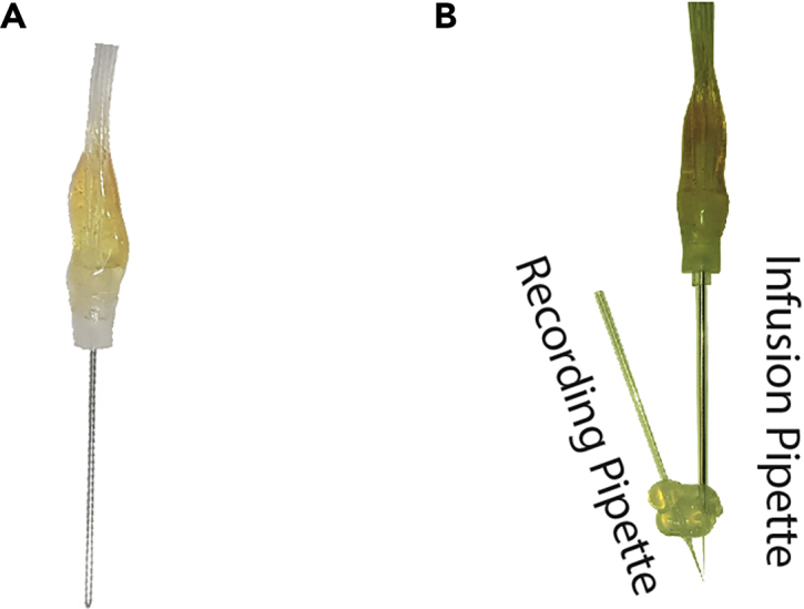
Figure 1.

Pipette pair assembly

(A) The produced pipette pair visualized under a microscope.

(B) Custom-made setup for pipette pair assembly. Pipettes are secured in the clamps; the recoding pipette is secured in the vertical clamp (Manipulator 1) and the infusion pipette is secured in the horizontal clamp (Manipulator 2) which moves back and forth as well as left to right. Under microscopic visualization and using Z nub, we first vertically align the recoding pipette with the infusion pipette; then, using nubs X (for back and forth movement) and Y (for left and right movement), the infusion pipette is juxtaposed to the recoding pipette. Finally, the pipettes are fixed together using a hot glue gun.

(C) Manipulator 1 (front view) with vertical clamps and the recording pipette.

(D) Manipulator 2 (top view) with horizontal clamp and the infusion pipette.

(E) An example pipette pair in the setup.

Induction of anesthesia

Timing: 15 min

• 4.Weigh the mouse on scale.
• 5.Anesthetize the mouse based on the protocol approved by the animal experimentation ethics committee. Below is the protocol we used.
• 6.Briefly anesthetize the mouse in isoflurane chamber for 2–5 min.
• 7.Administer 5 mL/kg of anesthetic solution intraperitoneally (ip).

Note: For studying the sensory processing in mammalian cortex, different anesthetic drugs are used which sometimes vary depending on the modality of interest. Based on our experience, urethane/chlorprothixene mixture provides a stable level of general anesthesia suitable for studying neuronal responses in the rodent somatosensory cortex.

• 8.Keep the mouse on the heating blanket.
• 9.Check the anesthetic level after 10–15 min by pinching the hind paw; if the mouse is not fully anesthetized, ip inject an additional dose of anesthetic solution equivalent to 10% of original dosage. If the mouse is fully anesthetized move to the next step.

Note: To achieve stable anesthesia by urethane, it is crucial that a correct ip injection is performed. Incorrect injection would result in slow absorption and may produce an unstable anesthesia.

Head fixation and craniotomy

Timing: 1 h

For head fixation we use a modified version of the setup described by Guo et al. (Guo et al., 2014). Here is a brief description of the head-fixation setup.

Note: The body temperature control system is compromised under anesthesia. It is therefore critical to keep the mouse on heating blanket during all stages of the experiment.

• 10.
  Head fixation (in brief)Proper head fixation is crucial for having a stable long-lasting recording from single neurons.

  • a.
    After ensuring that the mouse is fully anesthetized and while keeping the mouse on the heating blanket, remove the scalp to expose the frontal, parietal, and occipital bones.
  • b.
    Remove the periosteal tissue on the skull using forceps or by application of 1 mM hydrogen peroxide with a cotton bud.

    Note: Remember to remove the pieces of hair from the skull and thoroughly clean it.

  • c.
    Fix the head bar (Figure 2A) above Lambda using a thin layer of cyanoacrylate adhesive and dental acrylic (Vertex Self-Curing). Ensure the bone is dry before application of adhesive.
  • d.
    Let the cement set for at least 15 min.
  • e.
    Fix the head in the custom-made head post (Figure 2B).

• 11.
  Craniotomy

  Note: The position of craniotomy varies depending on the sensory modality of interest. Here, we focus on the vibrissal primary somatosensory cortex (vS1).

  • a.
    Mark the middle of vS1 on the skull based on its coordinates (1.8 mm posterior to bregma and 3.5 mm lateral from the midline suture).
  • b.
    Draw a 2 mm circle around that point for craniotomy.
  • c.
    Drill along the circular mark using a drill bit with 0.3 mm blunt head.
  • d.
    Apply ACSF regularly to clean the drilling area for better visualization and to avoid overheating the bone.
  • e.
    When the bone flap gets loose, it can be lifted up with a pair of forceps held horizontal to the skull.

    CRITICAL: Drill patiently while applying constant pressure. Drilling in one direction, either clockwise or anti-clockwise helps maintaining the uniformity of drilling and reduces the possibility of damaging the dura.

    Note: Remove the bone debris powder by flushing with ACSF and suctioning.

    Note: During this step, the bone may be detached from some areas but need more drilling in others. It is helpful to gently touch the bone flap with forceps to identify the areas that need further drilling.

  • f.
    In case of accidental damage to a blood vessel see Troubleshooting 1.
  • g.
    You need to keep the cortex always moist with regular application of ACSF.

    Note: At this stage, it is a good idea to fix the ground wire for electrophysiological recording. The wire should be placed away from the craniotomy area. We recommend inserting the wire between the muscles and the exposed skull.

Figure 2.

Head fixation and craniotomy

(A) After inducing anesthesia, scalp is removed and a head bar is attached to the skull.

(B) The head bar is fixed into a post to produce a stable head fixation for craniotomy.

Cortical infusion system

Timing: 10 min

You can use any pump to continuously inject the solution at rates of 1–10 μL/min. Here we use CMA 402 Syringe pumps and 1 mL glass syringes. We use 4 pumps and 4 syringes, 2 syringes for ACSF, 1 syringe each for agonist and antagonist solutions. Adjust the number of pumps based on the number of solutions. The tubes need to be connected at the infusion pipette level and transferred with a blunt needle gauge 21 to the tip of the infusion pipette (Figure 3A).

• 12.Fill the syringes with solutions.
• 13.Start running all pumps for several minutes to ensure every pump works properly.
• 14.Stop the pumps except the one filled with ACSF solution.

Note: You can do steps 12–14 while waiting for the cement to set after step 10d.

• 15.Fill the recording pipette with 5 μL of the recording solution; remove any potential air bubbles by gently flicking the pipette. Then fill the infusion pipette with 10–20 μL ACSF and remove any potential bubbles similar to before.
• 16.Insert the infusion needle to the infusion pipette and secure the end of pipette with the tube (Figure 3B).

Note: We use a blunt needle to transfer the solution faster to the tip of pipette. With the pump speed set at 3 μL/min, it usually took about 2–3 min for the solution to appear at the pipette tip.

• 17.Attach the recording pipette to the head stage.
• 18.Apply 250–300 mmHg pressure to the recording electrode to prevent contamination of the recording solution with ACSF.

Optional: The following step depends on the modality of interest. As we recorded from vS1, we used piezoelectric actuator connected to a mesh for whisker stimulation.

• 19.
  Attaching the piezoelectric actuator

  • a.
    Trim the contralateral whiskers to ∼3 mm using scissors.
  • b.
    Insert the whiskers into the mesh attached to the piezoelectric actuator (Figure 4A).

Note: The mesh should be close to the hair follicle but not touching the face of the animal. Ensure the piezoelectric actuator is ground shielded to reduce electrical noise.

CRITICAL: At any stage, it is important to not let the cortex dry out. Regularly apply ACSF on the exposed cortex.

Figure 3.

Infusion setup

(A) Blunt infusion needle to transfer solution to the tip of infusion pipette.

(B) Infusion pipette installation before the start of recording.

Figure 4.

Example outcome

(A) Schematic for application of sensory inputs (whisker stimulation) and recording/labeling of cortical neurons under pharmacological manipulation.

(B) Sensory-evoked neuronal responses increased by activating TRPA1 (red); the response levels decreased by introducing TRPA1 blocker (blue). This panel was adapted from Figure 1, Kheradpezhouh et al. (2020).

(C) Sensory-evoked responses increased by activating M1 AChR; the response levels decreased by inhibiting the receptor. In both (B) and (C), histological reconstruction of the recorded neuron is shown on the right column.

Juxtacellular recording/labeling

Timing: 2 h

Here, we followed the protocol described by Pinault, 1996 and modified in 2011 (Pinault, 1996, 2011).

• 20.Ensure that all the necessary equipment is connected and turned on. This includes amplifiers, sound system, micromanipulator, national instrument (NI) card and computers.
• 21.To penetrate the dura mater, apply constant pressure (of ∼300 mmHg) to the recording pipette and insert the pipette pair at a relatively fast speed of ∼100 μm/s.
• 22.After passing the dura, reduce the pressure to 10–20 mmHg and start searching for neurons at the slow speed of 1 μm/s. This can be done under current clamp mode with application of 1 nA pulses for 200 ms and 200 ms pause.
• 23.Continue the search until you identify a rise in impedance as the pipette comes in proximity of a neuron.
• 24.After reaching a neuron, remove the pressure and stop the current pulse.
• 25.Apply the sensory paradigm while recording the neuron. For example, in our experiments, we used a MATLAB (MathWorks, Inc., Natick, MA) script to present the stimuli and acquired the neuronal data through the analog input and output of a data acquisition card (National Instruments, Austin, TX). The whisker stimulation composed brief (20 ms) biphasic vertical movement generated by a piezoelectric actuator (Kheradpezhouh et al., 2017). The trials were presented in a pseudorandom order.
• 26.Apply agonist or antagonist by switching between the pumps.

Note: We applied the drugs for about 10–15 min each. This period should be optimized based on the specific drugs used in the experiment. In our experiments, it took 2–3 min for the drug to reach the neuron and we usually observed changes in neuronal response 5 min after switching between pumps.

• 27.
  After completing the experiment, load the neuron with neurobiotin as previously described (Pinault, 1996, 2011). Here in brief:

  • a.
    Apply 1-nA current pulses for 200 ms every 400 ms.
  • b.
    Increase the pulse amplitude 1 nA every 2–3 min until you observe the following changes in neuronal response which indicates the loading with neurobiotin.

Note: Systematic rise in the neuronal firing rate and broadening the action potential duration are the main 2 signs of successful loading with neurobiotin (Pinault, 1996, 2011). The other sign is the variability in amplitude and shape of neuronal action potential (Pinault, 1996, 2011). These signs usually disappear after you stop the current injection and allowing the neuron to rest for a few minutes.

• 28.After loading the neuron, detach from the neuron by applying 10–20 mmHg of pressure to the recoding pipette and slowly retract the pipette pair.

Note: If you want to record several neurons from each mouse, record the depth for each neuron to allow matching the recorded neurons with their histological reconstruction. For accurate identification of cell type, we recommend labeling a maximum of 3 neurons in each mouse.

• 29.Repeat these steps for the next experiment and neuron.

Harvesting the brain and immunostaining

• 30.After completing the recording experiment, cull the mouse by intraperitoneal administration of Lethabarb (150 mg/kg mouse weight).

Note: This step should be modified based on the protocol approved at your institute.

• 31.After the mouse stops breathing, open the abdomen and remove the anterior part of the chest.
• 32.Chop the liver to let the blood drain out.
• 33.Perform cardiac perfusion form the left ventricle with ∼10 mL of pre-chilled normal saline followed by ∼10 mL of 4% paraformaldehyde in PBS at the speed of ∼3 mL/min.
• 34.Harvest the brain and store in 4% PFA overnight (12–16 h) for fixation.
• 35.The next day, transfer the brain to PBS containing sequential sucrose solutions from 10% to 30% to achieve brain dehydration.
• 36.Embed the tissue in a Tissue-Tek mold using Tissue-Tek OCT compound and freeze the brain at −20°C for at least 1 h.
• 37.Section the brain at 100 μm thickness using a cryostat.
• 38.Incubate the sections in a 24-well plate.
• 39.Wash the sections with PBS 3 times 5 min each to ensure all remnants of the mounting medium have been rinsed off.
• 40.Incubate the slices in the penetration solution for ∼3 h.
• 41.Wash the sections with PBS 3 times 5 min each.

CRITICAL: The next steps need to be carried out in the dark.

• 42.Incubate the sections with PBS containing 0.1% Tween 20 and 1/1000 (v/v) Streptavidin conjugated with a secondary antibody overnight (12–16 h) at 4°C.
• 43.The next day, wash with PBS 3 times 5 min each.
• 44.Mount the sections on microscope slides, embedded in a mounting medium (Immumount) and cover with a coverslip.
• 45.Keep the section overnight (6–16 h) in a dark dry area.
• 46.Seal the edges with clear nail polish.
• 47.Use confocal microscopy to visualize the recorded neurons and capture images.

Note: During all incubations and washings, keep the slices on a shaker to increase the efficiency of binding.

Optional: Stain with DAPI (1:5,000) for 5 min to visualize cell nuclei of the loaded neuron.

Expected outcomes

Successful Juxtacellular recording captures the spiking activity of each neuron in response to various levels of sensory stimulation in the presence or absence of pharmacological manipulation. Here, to show the expected results, we draw 2 example recordings from the whisker area of the primary somatosensory cortex. Figures 4B and 4C illustrate the original response function of two example neurons to a range of whisker deflection amplitudes. Two example pharmacological modulations are shown: one for the transient receptor potential Ankyrin 1 (TRPA1, Figure 4B) and one for M1 acetylcholine receptor (Figure 4C).

Limitations

Pharmacological modulation: Effective and precise pharmacological modulation depends on the arrival of the drug onto the recorded neuron. As the infusion rate is low and the extent of pharmacological modulation is local, appropriate alignment of the pipettes is crucial for this type of experiment.

Limited number of recordings can be performed on each animal, as the pipette pair penetration damages the cortex more than conventional juxtacellular recordings with a single pipette. We recommend a maximum of 3–4 penetrations.

Matching the recorded neuron with its histological reconstruction: The matching becomes progressively more difficult as one increases the number of recorded/labeled neurons in each mouse. We recommend maximum 3 recordings from each animal. Documenting the depth of recording will help to identify the neuron.

Troubleshooting

Problem 1

Bleeding due to dura damage during craniotomy (step 11)

Potential solution

Apply ACSF to the bleeding area continuously and suction till the bleeding stops.

If bleeding is severe, you can use Gelfoam to gently absorb blood and to stop the bleeding.

Problem 2

Noisy recording – Some common sources of noise (steps 20–27)

Potential solution

All electrical devices can be a source of noise, including the lights, pumps, piezoelectric actuator, and the vacuum pumps. Check for any loose wiring around the setup and move the unnecessary equipment away from the recording set up.

Make sure all equipment are grounded.

Check the recording pipette carefully, as a slight damage to the pipette tip or its contamination can produce unstable recordings and noise. In this case, replace the pipette and try again.

Problem 3

Unable to find neurons (step 23)

Potential solution

Check the recording pipette before penetration; replace with a fresh pipette pair if broken or blocked.

The speed of infusion might be too high and may result in pushing neurons away from the pipette. Consider reducing the speed. We usually recorded at the infusion rate of 2–7 μL/min.

Problem 4

Losing neurons (steps 26 and 27)

Potential solution

After finding a neuron, if the amplitude of the recorded action potentials decreases over time, it could indicate that the infusion speed is too high. Consider reducing the speed of infusion by ∼0.5 μL/min or until the action potential amplitude is stabilized.

If reducing the speed does not solve the problem, consider replacing the pipette pair.

If the neuron is lost in the middle of a recording session, check the stability of the head fixation, anesthetic level, and look for potential pulsation movement in the brain.

Resource availability

Lead contact

Further information and requests for resources and reagents should be directed to and will be fulfilled by the lead contact, Ehsan Kheradpezhouh (ehsan.kheradpezhouh@anu.edu.au).

Materials availability

This study did not generate new unique reagents.

Data and code availability

This study did not generate any unique datasets or code.

The MATLAB codes generated during this study are available from lead contact on request.

References

- Guo Z.V., Hires S.A., Li N., O’Connor D.H., Komiyama T., Ophir E., Huber D., Bonardi C., Morandell K., Gutnisky D. Procedures for behavioral experiments in head-fixed mice. PLoS One. 2014;9:e88678. doi: 10.1371/journal.pone.0088678. [DOI] [PMC free article] [PubMed] [Google Scholar]
- Kheradpezhouh E., Adibi M., Arabzadeh E. Response dynamics of rat barrel cortex neurons to repeated sensory stimulation. Sci. Rep. 2017;7:11445. doi: 10.1038/s41598-017-11477-6. [DOI] [PMC free article] [PubMed] [Google Scholar]
- Kheradpezhouh E., Tang M.F., Mattingley J.B., Arabzadeh E. Enhanced sensory coding in mouse vibrissal and visual cortex through TRPA1. Cell Rep. 2020;32:107935. doi: 10.1016/j.celrep.2020.107935. [DOI] [PubMed] [Google Scholar]
- Pinault D. A novel single-cell staining procedure performed in vivo under electrophysiological control: Morpho-functional features of juxtacellularly labeled thalamic cells and other central neurons with biocytin or Neurobiotin. J. Neurosci. Methods. 1996;65:113–136. doi: 10.1016/0165-0270(95)00144-1. [DOI] [PubMed] [Google Scholar]
- Pinault D. The juxtacellular recording-labeling technique. Neuromethods. 2011;54:41–75. [Google Scholar]
- Schneider C.A., Rasband W.S., Eliceiri K.W. NIH Image to ImageJ: 25 years of image analysis. Nat. Methods. 2012;9:671–675. doi: 10.1038/nmeth.2089. [DOI] [PMC free article] [PubMed] [Google Scholar]
Associated Data
This section collects any data citations, data availability statements, or supplementary materials included in this article.
Data Availability Statement