Data-Driven Approaches to Predict Thermal Maturity Indices of Organic Matter Using Artificial Neural Networks

Abstract

Prediction of thermal maturity index parameters in organic shales plays a critical role in defining the hydrocarbon prospect and proper economic evaluation of the field. Hydrocarbon potential in shales is evaluated using the percentage of organic indices such as total organic carbon (TOC), thermal maturity temperature, source potentials, and hydrogen and oxygen indices. Direct measurement of these parameters in the laboratory is the most accurate way to obtain a representative value, but, at the same time, it is very expensive. In the absence of such facilities, other approaches such as analytical solutions and empirical correlations are used to estimate the organic indices in shale. The objective of this study is to develop data-driven machine learning-based models to predict continuous profiles of geochemical logs of organic shale formation. The machine learning models are trained using the petrophysical wireline logs as input and the corresponding laboratory-measured core data as a target for Barnett shale formations. More than 400 log data and the corresponding core data were collected for this purpose. The petrophysical wireline logs are γ-ray, bulk density, neutron porosity, sonic transient time, spontaneous potential, and shallow resistivity logs. The corresponding core data includes the experimental results from the Rock-Eval pyrolysis and Leco TOC measurements. A backpropagation artificial neural network coupled with a particle swarm optimization algorithm was used in this work. In addition to the development of optimized PSO-ANN models, explicit empirical correlations are also extracted from the fine-tuned weights and biases of the optimized models. The proposed models work with a higher accuracy within the range of the data set on which the models are trained. The proposed models can give real-time quantification of the organic matter maturity that can be linked with the real-time drilling operations and help identify the hotspots of mature organic matter in the drilled section.

1. Introduction

The depletion and fall of conventional oil and gas resources will lead to a shortage in the supply of the world’s energy needs.¹ Therefore, unconventional resources, in particular shale gas, are gaining popularity in the recent era of oil and gas.²⁻⁴ Organic-rich shale is one of the most vital sources of unconventional oil and gas. The appropriate geochemical characterization of shale resources plays a critical role in defining the prospect and development of the economic model of the field. For example, the production from Barnett Shale is controlled mainly by the thermal maturity, total organic carbon (TOC), and thickness of the shale target.⁵ The geochemical analysis aims to evaluate the organic richness, thermal maturity, and hydrocarbon potentiality of the organic-rich shale.⁶ The wettability and pore structure of the organic-rich shale are also affected by geochemical parameters.⁷

The most accurate estimation of the organic richness and thermal maturity of shale helps in reducing the risk carried by petroleum well drilling. Mineral heterogeneity, complex lithology, and natural fractures in shales have brought great challenges to the accurate estimation of the organic content.^8,9 Core measurements and well logs are the main ways to obtain geochemical parameters. Direct measurement of organic richness in the laboratory on the core samples is the most accurate way to obtain thermal maturity parameters. However, retrieving core samples from each well of every field and carrying out laboratory experiments on them is quite a time-consuming and costly method. Consequently, core-based geochemical data is very scarce. On the other hand, well log data is a prime component of all well drilling plans and hence is readily available. Limited core sample data and the associated well logs are used to develop correlations that can be applied to the whole well. Therefore, empirical correlations and machine learning-based models are used to obtain these parameters indirectly from well logs (need reference). The accuracy and applicability of these models depend on the data set and the region from where the data set is collected (need reference).

Machine learning (ML) and artificial intelligence (AI) both are the captivating fields that integrate computational power with human intelligence to produce smart and reliable solutions of extremely nonlinear and highly complicated problems.¹⁰ In the past two decades, engineering journals have reported numerous articles utilizing AI and ML for regression, function approximation, and classification problems.¹¹⁻¹³ With the advent of soft computing techniques, several correlations utilizing techniques from the field of AI have come to the fore, especially in reservoir characterization,¹⁴⁻¹⁶ reservoir engineering,¹⁷⁻²⁰ and reservoir geomechanics.^21,22 In petroleum geochemistry, such correlations can be seen in the works of Rahaman.²³ In recent years, support vector machine (SVM) and least-squares support vector machine techniques were actively used by researchers to predict total organic carbon (TOC);^24,25 researchers have used artificial neural networks too to predict TOC and thermal maturity.²⁶⁻²⁸

Based on the literature survey, it was observed that much attention was given to predict only the TOC content of the organic shales. However, organic matter geochemical analysis of shale gas formations requires estimation of a suite of parameters such as T_max, S₁, S₂, S₃, and TOC. Therefore, the objective of this study is to explore the potential of the machine learning technique in predicting these five geochemical parameters (T_max, S₁, S₂, S₃, and TOC) for the Barnett Shale. This study has utilized both machine learning and evolutionary algorithms to arrive at the optimum model. In addition to that, five explicit empirical correlations derived from the PSO-ANN algorithm are proposed; these correlations do not require any ML-based software for the execution.

1.1. Background

Geochemical properties of shale such as thermal maturity, source potentials (S₁–S₃), total organic carbon content (TOC), hydrogen index (HI), and oxygen index (OI) are important parameters to evaluate its production potential.^8,29S₁ and S₂ are called as volatile hydrocarbon and remaining hydrocarbon or oil potential, respectively.³⁰ The HI and OI are calculated from TOC and source potentials. Maximum temperature (T_max) is a chemical indicator of thermal maturity. T_max is the temperature at which the S₂ attains its maximum hydrocarbon generation.³¹ It accounts for the hydrogen and oxygen richness of the shale. On the other hand, TOC is an important indicator of organic richness in shale plays. TOC is expressed in weight percentage (wt %). Usually, if TOC is less than 0.5 wt %, it means no organic matter exists in the shale rock. A wt % of TOC greater than 0.5 is a positive sign for the existence of organic matter in shale rock. Several cross plots such as between T_max and hydrogen index (HI), S₂ and TOC, and HI and OI are used to evaluate the level of thermal maturity and kerogen type.³²⁻³⁴Table 1 presents the range of TOC and T_max according to the maturity level.

Table 1. TOC and T_max Range Describing the Level of Maturity.

parameter	no hydrocarbon	maturity range	postmaturity range	refs
TOC, wt %	less than 0.5	0.5–2	greater than 2	(35, 36)
Tmax, °C	less than 435	435–465	greater than 465	(33, 37)

There are three methods to determine geochemical parameters of organic-rich shale such as direct measurement, a single well log method,³⁸ and a composite well log method.³⁹ TOC can be measured directly in the laboratory in different ways such as filter acidification,⁴⁰ nonfilter acidification,⁴⁰ total minus coulometric,⁴¹ Rock-Eval,⁴² laser-induced pyrolysis,⁴³ and diffuse reflectance infrared Fourier transformation spectroscopy (DRIFTS).³⁴ Indirect methods involve the utilization of petrophysical well logs and seismic data. A large number of models are reported in the literature for the prediction of geochemical parameters using composite well logs.^{6,24−27,44−53}

Schmoker³⁸ established the first correlation to predict TOC for Devonian shale formation. Schmoker correlation is expressed in eq 1, which gives results in volume percentage

1

Schmoker⁵⁴ modified his correlation for Bakken formation as given by eq 2.

2

where ρ_o is the organic matter density in g/cm³, ρ_mi is the average density of grain and pore fluid in g/cm³, R_ρ is the ratio of the organic matter to organic carbon in weight percentage.

Passey et al.⁵⁵ suggested an easy-to-use model for TOC prediction, as summarized in eqs 3 and 4. Currently, this model is widely used for evaluating the unconventional resources reserve.

3

4

where R_baseline and R are the base formation and evaluated formation resistivities in Ω·m, respectively, Δ log R represents the log separation, Δt_baseline and Δt are the base formation and evaluated formation sonic transit times both in μs/ft, respectively, and LOM represents the formation level of maturity. Sultan²⁸ used a self-adaptive differential evolution algorithm to optimize artificial neural networks (ANN) and presented the empirical correlation to predict TOC of the Barnett shale. His correlation for TOC prediction is given by eqs 5–8

5

6

7

8

Table 2 presents some of the recent research works related to the prediction of organic matter in shale using machine learning and nonlinear regression approaches for the relevant geological fields.

Table 2. Summary of the Research Related to the Prediction of Organic Matter in Shale.

refs	study conducted	technique	method type	input parametersa	geological field study
Tan et al.24	prediction of TOC	artificial intelligence	epilson-SVR, nu-SCR, SMO-SVR, and RBF	CNL, GR, AC, K, TH, U, PE, RHOB, and RT	Huangping syncline, China
Rui et al.25	prediction of TOC	artificial intelligence	SVM	wireline log data such as RHOB, GR, SP, RT, and DT	Beibu Gulf basin
Lawal et al.27	prediction of TOC	artificial intelligence	ANN	XRD data: SiO2, Al2O3, MgO, and CaO	Devonian Shale
Sultan28	prediction of TOC	artificial intelligence	self-adaptive differential evolution-based ANN	well logs: GR, DT, RT, and RHOB	Devonian Shale
Mahmoud56	prediction of TOC	artificial intelligence	ANN	well logs: GR, DT, RT, and RHOB	Devonian Shale
Zhao et al.50	prediction of TOC	regression	nonlinear	CNL	Ordos Basin in China and Bakken Shale of North Dakota
Wang et al.53	prediction of TOC	regression	nonlinear	DT and RT	Sichuan Basin, Southern China
Alizadeh et al.46	prediction of TOC and S2	artificial intelligence	ANN	DT and RT	Dezful Embayment, Iran
Handhal et al.45	prediction of TOC	artificial intelligence	SVR, ANN, KNN, random forest, and rotation forest	GR, RHOB, NPHI, RllD, and DT	Rumaila Oil Field, Iran
Wang et al.48	TOC, S1, and S2	artificial intelligence	ANN	RHOB, NPHI, RT, and DT	Bohai Bay Basin, China

^aGR = γ-ray, RHOB = bulk density, LLD = deep lateral log, LLS = shallow lateral log, MSFL = microspherical focused log, R_ILD = deep induction resistivity log, DT = compressional wave travel time, TH = thorium, U = uranium, K = potassium, RT = resistivity log, NPHI = neutron porosity, SP = spontaneous potential, CNL = compensated neutron log, PE = photoelectric index, SiO₂ = silicondioxide, Al₂O₃ = aluminiumdioxide, MgO = magnesium oxide, and CaO = calcium oxide.

2. Results and Discussion

This section demonstrates the combined results for the prediction of five thermal maturity parameters such as T_max, S₁, S₂, S₃, and TOC. In this study, MATLAB, version 2020a was utilized to train models for thermal maturity of organic shales. An ANN is the stochastic learning technique that can generate nonunique results at every run. In this study, a seed number was assigned during each model run to obtain a unique result. A multiobjective function is defined using eq 9, which was designed to get the most accurate results during training and testing. Further improvement in results was done by coupling PSO with ANN.

9

where MAE_training^–1 is the inverse of the mean absolute error (MAE) during training, MAE_testing is the inverse of MAE testing, R_training² is the R² obtained during training, and R_testing is the R² obtained during testing. The inverse of MAE was taken to advance both MAE and R² in the same direction to get the maximum value for the objective function. The step-by-step pseudocode for the proposed PSO-ANN algorithm for thermal maturity parameter prediction is given in Table 3. Figure 1 shows the workflow chart of the proposed PSO-ANN algorithm to predict thermal maturity parameters.

Table 3. Step-by-Step Pseudocode for the Proposed PSO-ANN Algorithm for Thermal Maturity Parameter Prediction.

steps	working
1	start
2	set input variables
3	initialize parameters of ANN such as learning rate, activation functions, etc.
4	vary the number of hidden layers (sensitivity of hidden layers, 1–3)
5	vary the number of neurons in the hidden layer (sensitivity of neurons, 5–30)
5	select the learning algorithm of ANN
6	select the learning rate [0, 1] for the selected learning algorithm
7	train and test the ANN model and
8	evaluate the objective function for a minimum convergence value
9	extract weights and biases from the trained model
10	initialize parameters of PSO algorithm such as the number of iterations, population of particles, cognitive and social accelerations, and initial and final inertia weights
11	set range for sample search space of each extracted weights and biases
12	feed extracted weights and biases in a PSO algorithm as the initial population
13	evaluate the objective function for a minimum convergence value
14	run the iterative process until the stopping criteriona is achieved
15	pick the global best solution
16	set optimum weights and biases from the globally best model in the network for the prediction of thermal maturity parameters
17	end

^astopping criterion = a maximum number of iterations are attained or a maximum level of inactivity is reached.

Figure 1.

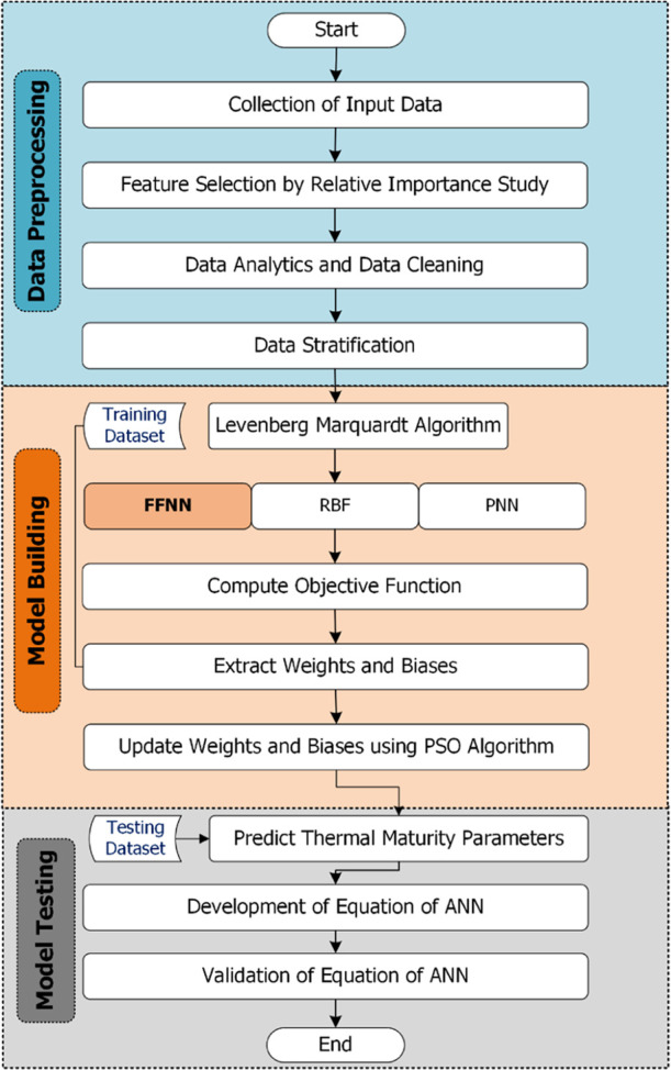
Workflow chart of the proposed PSO-ANN algorithm to obtain thermal maturity parameters.

In general, the trained ANN models for the prediction of thermal maturity of an organic shale comprised six input neurons such as GR, RHOB, DT, R_ILD, NPHI, and SP logs with ten middle-layer neurons. The number of neurons was chosen because of their best performance in terms of achieving maximum value of objective function defined in eq 16. Figure 2 shows the sensitivity of the number of neurons with the objective function. The middle layer with ten neurons was chosen because of their high performance. The general topology of the proposed model for the prediction of thermal maturity parameters is given in Figure 3, and the optimum values of the ANN technique for different models are listed in Table 4. The total data set for each model was stratified in the proportion of 70 and 30%. The 70% proportion was used for the training, and 30% was used for the testing of the trained model.

Figure 2.

Optimal number of neurons in the middle layer using an objective function.

Figure 3.

General topography of the proposed ANN model for the prediction of thermal maturity parameters.

Table 4. Optimum Values for the Proposed ANN Models.

parameters of the ANN model	range	Tmax	S1	S2	S3	TOC
number of input parameters	6	6	6	6	6	6
middle layer(s)	1–3	1	1	1	1	1
neurons in the middle layer	5–15	10	10	10	10	10
learning algorithm	quasi-newton, conjugate gradient, Levenberg–Marquardt (LM), Newton’s method, gradient descent (GD), resilient backpropagation (RB), Fletcher–Powell conjugate gradient, one-step secant	LM	RB	RB	LM	GD
rate of learning, α	0.1–0.5	0.15	0.2	0.10	0.16	0.18
middle-layer transfer function	tangential sigmoidal (tansig), logarithmic sigmoidal, hyperbolic sigmoidal, linear, rectified linear unit	tansig	tansig	tansig	tansig	tansig
epochs	100–500	150	115	125	180	260
outer-layer transfer function	linear	linear	linear	linear	linear	linear

For a T_max model, a total of 400 data points were obtained. On a training data set, the ANN model predicted the T_max with an R² of 0.917, an average absolute percentage error (AAAPE) of 1.006%, and a root-mean-square error (RMSE) of 0.258, while on a testing data set, the ANN model predicted the T_max with an R² of 0.918, an AAPE of 1.137%, and an RMSE of 0.428. The training and testing scatter plots are shown in Figure 4. The learning algorithm utilized was the LM with a learning rate of 0.15. With this combination, an optimum model was stored, and their weights and biases were extracted. The mathematical model for T_max utilizing optimum weights and biases is given in Appendix A.

Figure 4.

Training and testing of the T_max model.

For an S₁ model, a total of 400 data points was obtained. On a training data set, the ANN model predicted the S₁ with an R² of 0.919, an AAPE of 10.14%, and an RMSE of 0.003, while on a testing data set, the ANN model predicted the S₁ with an R² of 0.883, an AAPE of 12.232%, and an RMSE of 0.006. The training and testing scatter plots are shown in Figure 5. The learning algorithm utilized was the RB with a learning rate of 0.15. With this combination, an optimum model was stored, and their weights and biases were extracted. The mathematical model for S₁ utilizing optimum weights and biases is given in Appendix B.

Figure 5.

Training and testing of the S₁ model.

For an S₂ model, a total of 380 data points was obtained. On a training data set, the ANN model predicted the S₂ with an R² of 0.839, an AAPE of 13.8%, and an RMSE of 0.006, while on a testing data set, the ANN model predicted the S₂ with an R² of 0.827, an AAPE of 15.538%, and an RMSE of 0.010. The training and testing scatter plots are shown in Figure 6. The learning algorithm utilized was the RB with the learning rate of 0.15. With this combination, the optimum model was stored, and their weights and biases were extracted. The mathematical model for S₂ utilizing optimum weights and biases is given in Appendix C.

Figure 6.

Training and testing of the S₂ model.

For an S₃ model, a total of 450 data points was obtained. On a training data set, the ANN model predicted the S₃ with an R² of 0.891, an AAPE of 5.4%, and an RMSE of 0.001, while on a testing data set, the ANN model predicted the S₃ with an R² of 0.868, an AAPE of 6.11%, and an RMSE of 0.001. The training and testing scatter plots are shown in Figure 7. The learning algorithm utilized was the LM with the learning rate of 0.15. With this combination, the optimum model was stored, and their weights and biases were extracted. The mathematical model for S₃ utilizing optimum weights and biases is given in Appendix D.

Figure 7.

Training and testing of the S₃ model.

For a TOC model, a total of 360 data points were obtained. On a training data set, the ANN model predicted the TOC with an R² of 0.825, an AAPE of 7.863%, and an RMSE of 0.029, while on a testing data set, the ANN model predicted the TOC with an R² of 0.826, an AAPE of 8.713%, and an RMSE of 0.048. The training and testing scatter plots are shown in Figure 8. The learning algorithm utilized was GD with a learning rate of 0.15. With this combination, the optimum model was stored, and their weights and biases were extracted. The mathematical model for TOC utilizing optimum weights and biases is given in Appendix E.

Figure 8.

Training and testing of the TOC model.

To see the improvement in accuracy of the models using the proposed PSO-ANN-based algorithm, a comparison was made between conventional and PSO-ANN by comparing the R² obtained on overall data sets (training and testing). Figure 9 shows the bar chart that illustrates that in all five models (T_max, S₁, S₂, S₃, and TOC) the R² values obtained using the PSO-ANN algorithm were much higher than the conventional ANN model. This proves that the proposed PSO-ANN algorithm-based models have much higher accuracy than the models based on the conventional ANN technique.

Figure 9.

Comparison of conventional ANN and PSO-ANN in terms of the coefficient of determination on an overall data set.

3. Conclusions

A good estimation of shale geochemical properties requires a sophisticated approach. Minor variations in anticipated results lead to wastage of man-hours and huge investments. On the other hand, a small improvement in the estimation practices can improve the worth of the exploration project manyfold. The development of robust and improved models for prediction of thermal maturity of organic shale was the focus of this study. To achieve the objective, an ANN tool coupled with a PSO algorithm is employed in this work. The evaluation of the proposed models was based on various statistical measures such as RMSE, AAPE, MAE, and R². A step-by-step comprehensive analysis to reach the optimum model selection along with the statistical and graphical metrics was also presented in this study. The generalization capability of the proposed models was tested using a blind data set. By correlating the predicted maturity index with the core-based one, the proposed models were found to be effective, faster, and more readily available than lab analysis. The proposed models are completely reproducible. The proposed PSO-ANN-based models can give reliable predictions in the absence of experimental data and therefore can be a good choice to be included in any software package for a complete analysis of geochemical data without going to the laboratory for carrying out the Rock-Eval pyrolysis experiment. The proposed models can give real-time quantification of organic matter maturity using readily available well logs that can help us to identify the hotspots of mature organic matter in the drilled section.

4. Materials and Methods

4.1. Studied Geological Field

The Mississippian Barnett Shale in Fort Worth Basin, North Texas is a classic world-class unconventional shale gas reservoir.⁵⁷ It consists mainly of silica-rich mudstone interlaminated with clay- and calcareous-rich mudstone and deposited in a low-energy, relatively deep water environment.^35,58 The subsurface thickness of Barnett Shale reaches up to about 1000 ft. (304.8 m) in the Newark sub-basin. In the Newark East field, from where the data comes, Barnett Shale is thermally mature, averaging 4–5 wt % total organic carbon TOC, and trapped between two impermeable limestone beds, which is the most favorite conditions for vertical well completion. However, the variation in the thickness, mineral composition, organic richness, and thermal maturity levels through the entire Fort Worth Basin raised the need to reduce the uncertainty of predicted reservoir properties in the rest of the basin and develop AI models that can be applied to another shale gas reservoirs.

4.2. Geochemical Analysis

Pyrolysis is a process of performing thermal decomposition of materials at higher temperatures. The geochemical analysis of an organic matter is comprised of Rock-Eval pyrolysis. Pyrolysis is used to evaluate the thermal maturity and organic richness of the source rock. From the pyrolysis experiment, the quality, quantity type, thermal maturity, hydrogen index, migration index, production index, and oxygen index of organic matter can be determined. Typically, the five parameters T_max, S₁, S₂, S₃, and TOC are measured. S₁ accounts for free hydrocarbon released at 300°C measured in mg HC/g rock. S₂ accounts for hydrocarbon released from the cracking of kerogen at the temperature range between 300 and 600 °C measured in mg HC/g rock. S₃ accounts for carbon dioxide (CO₂) released from the breaking of carboxy groups and other oxygen-containing compounds measured in mg CO₂/g rock. The TOC is measured by oxidizing the residue left in the pyrolysis process at a fixed temperature of 600 °C.^6,36Figure 10 shows the schematic of the different fractions obtained from total organic matter.

Figure 10.

Diagram showing the fractions of the total organic matter.

4.3. Data Analytics

The statistical description of the data set used to train AI models for the geochemical parameters prediction is given in Table 5. The ranges of the input parameters for each model are quite practically reasonable. The complete data set utilized for the training of each model is given in Figure 11.

Table 5. Ranges of the Data Used for AI Modeling.

	GR, API		RHOB (g/cc)		NPHI (vol/vol)		RILD, (Ω–m)		Δtc (μs/ft)		SP (mV)
models	min	max	min	max	min	max	min	max	min	max	min	Max
Tmax (°C)	18.229	417.06	2.37	2.86	0.003	0.33	4.8	1283.34	45.27	93.48	–154.18	–28.62
S1 (mg HC/g rock)	19.120	336.73	2.37	2.86	0.003	0.33	1.3	1027.90	45.27	93.39	–154.18	–28.62
S2 (mg HC/g rock)	18.229	372.29	2.37	2.86	0.003	0.33	1.3	1283.34	45.27	93.39	–154.18	–28.81
S3 (mg CO2/g rock)	18.229	417.06	2.37	2.83	0.003	0.29	4.8	1088.66	45.27	92.08	–154.18	–28.81
TOC (wt %)	55.500	359.76	2.20	2.68	0.03	0.33	6.0	148.87	62.05	93.39	–86.69	–29.25

Figure 11.

Well logs’ input data (AT90 is a R_ILD log).

The core data of the corresponding conventional wireline well logs are collected. The frequency distribution of the measured T_max, S₁, S₂, S₃, and TOC from the geochemical analysis is shown in Figure 12. The T_max data is evenly distributed over a wide range between 420 and 540 °C. S₁ is mainly distributed between 0.1 and 1. S₂ is mainly distributed between 0.3 and 1.6. About 60% of the cores have an S₂ lower than 1, and only a few have permeability above 1.5. The S₃ data is uniformly distributed over a range between 0.1 and 0.3. The TOC data is mainly distributed between 2 and 6, with only fewer points above 6. The frequency histograms show that the core data values are distributed over a wide range of values and are quite heterogenous.

Figure 12.

Frequency distribution of T_max, S₁, S₂, S₃, and TOC.

4.4. Feature Selection

Feature selection was made by evaluating the relative importance of the input parameters with the output parameter using the Pearson correlation coefficient (CC) criterion, which is given by eq 10

10

where x and y are two variables and k is the sample size. The value of CC lies between −1 and +1. The values near to negative one show an inverse relationship between two variables, the values near to the positive one show a direct relationship between two variables, and the values near to zero show a poor relationship between the pair of two variables. Figure 13 shows the CC of input parameters such as GR, RHOB, NPHI, AT90, Δt_c, and SP log with the target parameters such as T_max, S₁, S₂, S₃, and TOC.

Figure 13.

Relative importance of the input parameters such as GR, ρ, NPHI, AT90 (R_ILD), Δt_c, and SP logs with the output parameters such as T_max, S₁, S₂, S₃, and TOC.

4.5. Accuracy Metrics

The models were evaluated based on the goodness-of-fit tests such as the average absolute percentage error (AAPE), mean absolute error (MAE), root-mean-square error (RMSE), and coefficient of determination (R²). The definition of these parameters is given in Table 6.

Table 6. Statistical Indicators of Model Performance Evaluation^a.

goodness-of-fit test	mathematical expression
average absolute percentage error	11
mean absolute error	12
root-mean-square error	13
coefficient of determination	14

^aY_measured is the measured value of TOC, Y_predicted is the estimated value from the model, and n is the total number of samples.

4.6. Machine Learning Method

Artificial neural network (ANN) is a machine learning (ML) technique, mostly used for function approximation purposes. It is comprised of a series of layers such as an input layer, a middle layer(s), and an output layer. The middle layer is also called a hidden layer and it can be single or multiple, depending on the training data set.⁵⁹ The selection of the number of neurons in the middle layers depends on the overall model performance in terms of accuracy.⁶⁰ A transfer function exists between the input layer and the middle layer, and another transfer function exists between the middle layer and the output layer. Various choices of transfer functions are available such as linear, sigmoidal, radial basis, and rectified linear unit (ReLU) type. The detailed description of the theory and utilization of ANN can be found in our previous publications.^10,61,62

Particle swarm optimization (PSO) is utilized to optimize the weights and biases of a neural network. In the past, many researchers have found good results by coupling PSO with other AI techniques such as ANN, least-squares support vector machine (LSSVM), and adaptive neuro-fuzzy inference system (ANFIS).⁶³⁻⁶⁷ PSO is an evolutionary algorithm (EA) inspired by the social movement of birds and fish. EA algorithms are based on the stochastic approach that looks for the best possible solution in the search space. The PSO algorithm depends on four parameters that are population size, weight, particle velocity, and cognitive parameters. A detailed discussion about the PSO algorithm can be found in the publication of Abido.⁶⁸ Particles velocity term is given by eq 15

15

where w is the weight of the particle (0 ≤ w ≤ 1.2), v_i is the particle velocity, c₁ is the cognitive parameter (0 ≤ c₁ ≤ 1.2), c₂ is the cognitive parameter (0 ≤ c₂ ≤ 1.2), n is the number of iteration, p_i^b is the local best solution of the particle, p_gb is the global best solution of the particle, and p_i is the ith position of the particle at the nth iteration. The next position for each candidate solution in the search space is created by summation of the current particle position and particle velocity

16

Glossary

Abbreviations Used

AAPE

average absolute percentage error

ANFIS

adaptive neuro fuzzy inference system

ANN

artificial neural network

CC

correlation coefficient

CNL

compensated neutron log

DT

compressional wave travel time

EA

evolutionary algorithm

GR

γ-ray, API

K

potassium

LLD

deep lateral log

LLS

shallow lateral log

LSSVM

least-squares support vector machine

MAE

mean absolute error

ML

machine learning

MLR

multiple linear regression

MSFL

microspherical focused log

NPHI

neutron porosity, V/V

PE

photoelectric index

PSO

particle swarm optimization

R

correlation coefficient

R²

coefficient of determination

RHOB

bulk density

R_ILD

deep induction resistivity log

RMSE

root-mean-square error

RT

resistivity log

SD

standard deviation

SP

spontaneous potential

SVM

support vector machine

TH

thorium

U

uranium

Glossary

Symbols

α

learning rate

b₁

biases vector between the input and middle layers

b₂

bias value between the middle and output layers

c₁

cognitive parameter (0 ≤ c₁ ≤ 1.2)

c₂

cognitive parameter (0 ≤ c₂ ≤ 1.2)

i

index used for the total number of neurons

j

index used for the number of inputs

J

total number of input parameters

n

normalized value

N_h

total number of neurons

N_p

total number of input parameters

_pi

position of the ith particle

_pi^b

best solution of the particle

p_gb

global best solution

R²

coefficient of determination

v_i

particle velocity

w₁

weights matrix between the input and middle layers

w₂

weights vector between the middle and output layers

x

input parameters

y

output variable

σ_o

transfer function between the middle and output layers

σ_L

transfer function between the input and middle layers

ω

weight (0 ≤ w ≤ 1.2)

Appendix A Mathematical Model to Predict T_max

The ANN-based mathematical model to predict the T_max of the organic shale is given by eq AA1

A1

where

A2

where σ_L(x) = (2/1 + e^–2x) – 1; σ_o(x) = x; and w₁, w₂, b₁, and b₂ are the weights and biases of the T_max model, given in Table 7. GR_n is the normalized value of a γ-ray log, ρ_n is a normalized value of a bulk density, φ_n is a normalized value of a neutron porosity, R_ILDn is a normalized value of a R_ILD resistivity log, Δt_Cn is a normalized value of a compressional wave travel time, SP_n is a normalized value of an SP log. The equations to find GR_n, ρ_n, φ_n,R_ILDn, Δt_Cn, and SP_n are given by eqs AA3–AA7.

A3

where GR is the γ-ray log in API.

A4

where ρ is the bulk density in g/cc.

A5

where φ is the neutron porosity.

A6

where R_ILD is the resistivity log in Ω·m.

A7

where Δt_C is the compressional wave travel time in μs/ft.

A8

where SP is the spontaneous potential log in mV.

Table 7. Weights and Biases of the Proposed Model for T_max Prediction.

	weights between input and hidden layers (w1)
hidden layer neurons (Nh)	GR	ρ	NPHI	RILD	ΔtC	SP	weights between hidden and output layers (w2)	hidden layer bias (b1)	output layer bias (b2)
1	–1.7941	0.2967	0.2405	3.9757	–0.6821	0.1778	–1.7717	5.1003	1.4308
2	–2.0779	0.8055	1.2726	–0.5317	–0.2028	–0.3555	2.9596	1.0329
3	–0.2541	–1.2323	2.3337	–0.0487	4.0613	1.0812	0.5933	6.0397
4	0.1803	–1.5660	–0.7003	1.9781	0.3196	0.4630	–1.3631	2.3029
5	–1.8247	0.7878	2.1122	1.7892	0.2356	2.8205	1.0260	–2.4688
6	0.8137	–1.3633	–0.8132	1.1902	–0.4400	0.0050	2.5527	1.4510
7	–0.4772	–3.1851	–0.8343	0.4839	0.3739	–3.1749	–0.5414	0.1539
8	–1.1043	3.5500	–3.5252	–0.9498	2.1798	4.9600	–0.1921	–3.1789
9	–1.7033	0.4957	–0.6426	–0.4278	–1.3891	0.1037	1.8245	–4.7481
10	2.3884	–2.4291	1.0258	–0.2708	–4.4849	2.0855	–0.4637	1.1179

Appendix B Mathematical Model to Predict S₁

The ANN-based mathematical model to predict the S₁ of the organic shale is given by eq BB1

B1

B2

where σ_L(x) = (2/1 + e^–2x) – 1; σ_o(x) = x; and w₁, w₂, b₁, and b₂ are the weights and biases of the S₁ model, given in Table 8. The equations to find GR_n, ρ_n, φ_n, R_ILDn, Δt_Cn, and SP_n are given by eqs BB3–BB7.

B3

where GR is the γ-ray log in API.

B4

where ρ is the bulk density in g/cc.

B5

where φ is the neutron porosity.

B6

where R_ILD is the resistivity log in Ω–m.

B7

where Δt_C is the compressional wave travel time in μs/ft.

B8

where SP is the spontaneous potential log in mV.

Table 8. Weights and Biases of the proposed Model for S₁ Prediction.

	weights between input and hidden layers (w1)
hidden layer neurons (Nh)	GR	ρ	NPHI	RILD	ΔtC	SP	weights between hidden and output layers (w2)	hidden layer bias (b1)	output layer bias (b2)
1	–0.0872	2.3795	0.61	0.9346	–1.0302	2.6013	2.2032	2.7471	–1.125
2	2.9553	1.196	0.9532	–0.1497	2.0403	–0.6852	–1.5668	3.5566
3	0.9799	–2.0489	–0.5193	1.0599	1.1969	3.2706	–2.0522	–0.5307
4	–0.3019	1.5661	0.1572	0.0954	0.0242	–2.0559	–3.1289	1.1359
5	1.8638	–0.8322	–3.3966	0.6946	2.8564	3.4534	–1.377	–3.9418
6	–3.2506	0.8794	1.5293	1.2903	0.8682	0.4842	–3.4481	–0.2281
7	1.7284	–1.3916	4.3578	–2.3109	–5.3719	0.012	–1.0532	0.6863
8	–2.3325	0.5383	1.3951	–0.8393	0.687	0.3473	3.2165	–2.2594
9	0.6438	1.1076	3.1629	0.6633	0.8062	–0.8584	1.4581	3.789
10	1.7403	–1.5715	1.5465	–2.1928	–0.0194	–2.249	–0.7571	1.6332

Appendix C Mathematical Model to Predict S₂

The ANN-based mathematical model to predict the S₂ of the organic shale is given by eq CC1

C1

C2

where σ_L(x) = (2/1 + e^–2x) – 1; σ_o(x) = x; and w₁, w₂, b₁, and b₂ are the weights and biases of the S₂ model, given in Table 9. The equations to find GR_n, ρ_n, φ_n, R_ILDn, Δt_Cn, and SP_n are given by eqs CC3–CC7.

C3

where GR is the γ-ray log in API.

C4

where ρ is the bulk density in g/cc.

C5

where φ is the neutron porosity.

C6

where R_ILD is the resistivity log in Ω·m.

C7

where Δt_C is the compressional wave travel time in μs/ft.

C8

where SP is the spontaneous potential log in mV.

Table 9. Weights and Biases of the Proposed Model for S₂ Prediction.

	weights between input and hidden layers (w1)
hidden layer neurons (Nh)	GR	ρ	NPHI	RILD	ΔtC	SP	weights between hidden and output layers (w2)	hidden layer bias (b1)	output layer bias (b2)
1	–3.615	–3.658	5.426	1.372	2.019	–5.133	–0.406	–2.487	0.711
2	5.917	–0.778	1.821	1.348	–2.140	1.007	–0.509	5.152
3	–2.575	–0.020	1.776	–0.650	–1.119	1.817	5.629	–0.469
4	–0.339	0.970	–1.707	–1.300	–0.551	–0.881	1.030	–0.459
5	–0.890	–0.478	0.944	–9.386	–0.114	2.103	2.762	–11.697
6	–1.869	0.389	0.903	1.473	0.715	–0.465	2.594	1.915
7	1.196	–9.027	–3.565	1.744	–4.834	–6.791	–0.331	1.166
8	–2.109	1.027	0.875	0.538	1.649	–0.208	–2.602	0.392
9	–1.703	–0.176	1.199	–0.617	–1.307	1.459	–6.972	–0.500
10	4.054	–6.402	–1.309	–5.677	–6.265	17.736	0.621	–10.018

Appendix D Mathematical Model to Predict S₃

The ANN-based mathematical model to predict the S₃ of the organic shale is given by eq DD1

D1

where

D2

where σ_L(x) = (2/1 + e^–2x) – 1; σ_o(x) = x; and w₁, w₂, b₁, and b₂ are the weights and biases of the S₃ model, given in Table 10. The equations to find GR_n, ρ_n, φ_n, R_ILDn, ΔT_Cn, and SP_n are given by eqs DD3–DD7.

D3

where GR is the γ-ray log in API.

D4

where ρ is the bulk density in g/cc.

D5

where φ is the neutron porosity.

D6

where R_ILD is the resistivity log in Ω·m.

D7

where Δt_C is the compressional wave travel time in μs/ft.

D8

where SP is the spontaneous potential log in mV.

Table 10. Weights and Biases of the Proposed Model for S₃ Prediction.

	weights between input and hidden layers (w1)
hidden layer neurons (Nh)	GR	ρ	NPHI	RILD	ΔtC	SP	weights between hidden and output layers (w2)	hidden layer bias (b1)	output layer bias (b2)
1	–1.366	–0.203	0.630	–0.508	–1.215	–1.586	–2.372	2.103	–2.081
2	0.248	0.581	–0.757	–4.469	0.632	1.145	3.125	–3.801
3	–1.266	3.104	2.077	–0.856	–1.393	–2.028	0.958	1.611
4	–0.034	–0.877	0.945	–4.088	–0.183	0.358	2.039	–3.462
5	–0.485	0.079	2.798	–0.098	–2.098	–2.592	1.451	–1.440
6	–0.131	1.104	–0.111	0.917	–1.104	–0.280	3.982	0.190
7	0.006	0.473	0.145	–3.503	–0.081	0.578	–3.989	–3.248
8	0.342	0.235	–0.188	–0.969	–1.883	0.090	–2.849	–1.548
9	0.459	–0.080	1.096	–1.149	–1.765	2.086	2.723	1.431
10	–1.719	–0.903	–2.539	0.334	–3.960	0.820	0.985	4.271

Appendix E Mathematical Model to Predict Total Organic Carbon

The ANN-based mathematical model to predict the S₃ of the organic shale is given by eq EE1

E1

where

E2

where σ_L(x) = (2/1 + e^–2x) – 1; σ_o(x) = x; and w₁, w₂, b₁, and b₂ are the weights and biases of the TOC model, given in Table 11. The equations to find GR_n, ρ_n, φ_n, R_ILDn, ΔT_Cn, and SP_n are given by eqs EE3–EE7.

E3

where GR is the γ-ray log in API.

E4

where ρ is the bulk density in g/cc.

E5

where φ is the neutron porosity.

E6

where R_ILD is the resistivity log in Ω·m.

E7

where Δt_C is the compressional wave travel time in μs/ft.

E8

where SP is the spontaneous potential log in mV.

Table 11. Weights and Biases of the Proposed Model for TOC Prediction.

	weights between input and hidden layers (w1)
hidden layer neurons (Nh)	GR	ρ	NPHI	RILD	ΔtC	SP	weights between hidden and output layers (w2)	hidden layer bias (b1)	output layer bias (b2)
1	1.759	–1.040	1.233	2.680	–0.320	–1.225	1.372	–1.683	1.923
2	0.875	0.288	0.309	–1.399	–0.701	0.682	4.431	–0.756
3	0.990	–0.414	–1.286	–1.252	–0.283	3.069	–1.250	–1.101
4	–1.100	–1.601	–1.629	–3.078	0.297	–0.882	1.538	–3.488
5	2.962	–1.130	0.781	–2.217	–1.349	0.861	–0.787	0.840
6	–0.886	1.227	0.386	6.639	2.619	–3.780	1.059	2.219
7	0.417	–1.863	0.815	–0.082	1.125	–1.183	–1.524	2.046
8	–0.847	–1.005	0.479	0.991	0.410	0.273	–0.556	–2.068
9	–0.606	–1.045	–1.203	0.960	1.449	0.264	2.000	1.132
10	2.624	–2.675	–0.025	–0.704	0.800	–1.333	1.013	3.426

The authors declare no competing financial interest.

Author Status

^† At time of publication, M.A. is on sabbatical leave from Faculty of Petroleum & Mining Engineering, Suez University, Egypt.

References

- Sharma S.; Agrawal V.; Akondi R. N. Role of Biogeochemistry in Efficient Shale Oil and Gas Production. Fuel 2020, 259, 116207 10.1016/j.fuel.2019.116207. [DOI] [Google Scholar]
- Hosseini H.; Tsau J. S.; Shafer-Peltier K.; Marshall C.; Ye Q.; Ghahfarokhi R. B. Experimental and Mechanistic Study of Stabilized Dry CO2 Foam Using Polyelectrolyte Complex Nanoparticles Compatible with Produced Water to Improve Hydraulic Fracturing Performance. Ind. Eng. Chem. Res. 2019, 58, 9431–9449. 10.1021/acs.iecr.9b01390. [DOI] [Google Scholar]
- Lee K. S.; Kim T. H.. Integrative Understanding of Shale Gas Reservoirs; Springer, 2016. [Google Scholar]
- Ahmed S.; Sri Hanamertani A.; Rehan Hashmet M.. CO 2 Foam as an Improved Fracturing Fluid System for Unconventional Reservoir. In Exploitation of Unconventional Oil and Gas Resources - Hydraulic Fracturing and Other Recovery and Assessment Techniques; IntechOpen, 2019; pp 1–24. [Google Scholar]
- Zhao H.; Givens N. B.; Curtis B. Thermal Maturity of the Barnett Shale Determined from Well-Log Analysis. AAPG Bull. 2007, 91, 535–549. 10.1306/10270606060. [DOI] [Google Scholar]
- Jarvie D. M.; Hill R. J.; Ruble T. E.; Pollastro R. M. Unconventional Shale-Gas Systems: The Mississippian Barnett Shale of North-Central Texas as One Model for Thermogenic Shale-Gas Assessment. AAPG Bull. 2007, 91, 475–499. 10.1306/12190606068. [DOI] [Google Scholar]
- Zhang T.; Ellis G. S.; Ruppel S. C.; Milliken K.; Yang R. Effect of Organic-Matter Type and Thermal Maturity on Methane Adsorption in Shale-Gas Systems. Org. Geochem. 2012, 47, 120–131. 10.1016/j.orggeochem.2012.03.012. [DOI] [Google Scholar]
- Gale J. F. W.; Reed R. M.; Holder J. Natural Fractures in the Barnett Shale and Their Importance for Hydraulic Fracture Treatments. AAPG Bull. 2007, 91, 603–622. 10.1306/11010606061. [DOI] [Google Scholar]
- Vöröš D.; Geršlová E.; Díaz-Somoano M.; Sýkorová I.; Suárez-Ruiz I.; Havelcová M.; Kuta J. Distribution and Mobility Potential of Trace Elements in the Main Seam of the Most Coal Basin. Int. J. Coal Geol. 2018, 196, 139–147. 10.1016/j.coal.2018.07.005. [DOI] [Google Scholar]
- Tariq Z.; Mahmoud M.; Abdulraheem A. Core Log Integration: A Hybrid Intelligent Data-Driven Solution to Improve Elastic Parameter Prediction. Neural Comput. Appl. 2019, 31, 8561–8581. 10.1007/s00521-019-04101-3. [DOI] [Google Scholar]
- Gao W.; Chen X.; Chen D. Genetic Programming Approach for Predicting Service Life of Tunnel Structures Subject to Chloride-Induced Corrosion. J. Adv. Res. 2019, 20, 141–152. 10.1016/j.jare.2019.07.001. [DOI] [PMC free article] [PubMed] [Google Scholar]
- Samui P.; Hariharan R. A Unified Classification Model for Modeling of Seismic Liquefaction Potential of Soil Based on CPT. J. Adv. Res. 2015, 6, 587–592. 10.1016/j.jare.2014.02.002. [DOI] [PMC free article] [PubMed] [Google Scholar]
- Ghanem T. F.; Elkilani W. S.; Abdul-kader H. M. A Hybrid Approach for Efficient Anomaly Detection Using Metaheuristic Methods. J. Adv. Res. 2015, 6, 609–619. 10.1016/j.jare.2014.02.009. [DOI] [PMC free article] [PubMed] [Google Scholar]
- Anifowose F. A.; Labadin J.; Abdulraheem A. Ensemble Machine Learning: An Untapped Modeling Paradigm for Petroleum Reservoir Characterization. J. Pet. Sci. Eng. 2017, 151, 480–487. 10.1016/j.petrol.2017.01.024. [DOI] [Google Scholar]
- Anifowose F.; Abdulraheem A. Fuzzy Logic-Driven and SVM-Driven Hybrid Computational Intelligence Models Applied to Oil and Gas Reservoir Characterization. J. Nat. Gas Sci. Eng. 2011, 3, 505–517. 10.1016/j.jngse.2011.05.002. [DOI] [Google Scholar]
- Anifowose F.; Labadin J.; Abdulraheem A. Improving the Prediction of Petroleum Reservoir Characterization with a Stacked Generalization Ensemble Model of Support Vector Machines. Appl. Soft Comput. 2015, 26, 483–496. 10.1016/j.asoc.2014.10.017. [DOI] [Google Scholar]
- Al-Marhoun M. A.; Osman E. A. In Using Artificial Neural Networks to Develop New PVT Correlations for Saudi Crude Oils, Abu Dhabi International Petroleum Exhibition and Conference; Society of Petroleum Engineers, 2002.
- Gharbi R. B.; Elsharkawy A. M.; Karkoub M. Universal Neural-Network-Based Model for Estimating the PVT Properties of Crude Oil Systems. Energy and Fuels 1999, 13, 454–458. 10.1021/ef980143v. [DOI] [Google Scholar]
- Gharbi R. B.; Elsharkawy A. M. In Neural Network Model for Estimating the PVT Properties of Middle East Crude Oils, Proceedings of the Middle East Oil Show; Society of Petroleum Engineers, 1997; Vol. 1, pp 151–166.
- Khan M. R.; Tariq Z.; Abdulraheem A. Application of Artificial Intelligence to Estimate Oil Flow Rate in Gas-Lift Wells. Nat. Resour. Res. 2020, 1–13. 10.1007/s11053-020-09675-7. [DOI] [Google Scholar]
- Tariq Z.; Abdulraheem A.; Mahmoud M.; Ahmed A. A Rigorous Data-Driven Approach to Predict Poisson’s Ratio of Carbonate Rocks Using a Functional Network. Petrophysics 2018, 59, 761–777. 10.30632/PJV59N6-2018a2. [DOI] [Google Scholar]
- Tariq Z.; Mahmoud M. A.; Abdulraheem A.; Al-Shehri D. A. In On Utilizing Functional Network to Develop Mathematical Model for Poisson’s Ratio Determination, 52nd U.S. Rock Mechanics/Geomechanics Symposium; American Rock Mechanics Association: Seattle, Washington, 2018.
- Rahaman M. S. A.; Vasant P.. Artificial Intelligence Approach for Predicting TOC From Well Logs in Shale Reservoirs; IGI Global, 2020; pp 46–77. [Google Scholar]
- Tan M.; Song X.; Yang X.; Wu Q. Support-Vector-Regression Machine Technology for Total Organic Carbon Content Prediction from Wireline Logs in Organic Shale: A Comparative Study. J. Nat. Gas Sci. Eng. 2015, 26, 792–802. 10.1016/j.jngse.2015.07.008. [DOI] [Google Scholar]
- Rui J.; Zhang H.; Zhang D.; Han F.; Guo Q. Total Organic Carbon Content Prediction Based on Support-Vector-Regression Machine with Particle Swarm Optimization. J. Pet. Sci. Eng. 2019, 180, 699–706. 10.1016/j.petrol.2019.06.014. [DOI] [Google Scholar]
- Khoshnoodkia M.; Mohseni H.; Rahmani O.; Mohammadi A. TOC Determination of Gadvan Formation in South Pars Gas Field, Using Artificial Intelligent Systems and Geochemical Data. J. Pet. Sci. Eng. 2011, 78, 119–130. 10.1016/j.petrol.2011.05.010. [DOI] [Google Scholar]
- Lawal L. O.; Mahmoud M.; Saheed Alade O.; Abdulraheem A. Total Organic Carbon Characterization Using Neural-Network Analysis of XRF Data. Petrophysics 2019, 60, 480–493. 10.30632/PJV60N4-2019a2. [DOI] [Google Scholar]
- Sultan A. In New Artificial Neural Network Model for Predicting the TOC from Well Logs, SPE Middle East Oil and Gas Show and Conference; Society of Petroleum Engineers, 2019.
- Mendhe V. A.; Mishra S.; Varma A. K.; Kamble A. D.; Bannerjee M.; Singh B. D.; Sutay T. M.; Singh V. P. Geochemical and Petrophysical Characteristics of Permian Shale Gas Reservoirs of Raniganj Basin, West Bengal, India. Int. J. Coal Geol. 2018, 188, 1–24. 10.1016/j.coal.2018.01.012. [DOI] [Google Scholar]
- Yu F.; Sun P.; Zhao K.; Ma L.; Tian X. Experimental Constraints on the Evolution of Organic Matter in Oil Shales during Heating: Implications for Enhanced in Situ Oil Recovery from Oil Shales. Fuel 2020, 261, 116412 10.1016/j.fuel.2019.116412. [DOI] [Google Scholar]
- Ahmed M. A.; Hassan M. M. A. Hydrocarbon Generating-Potential and Maturity-Related Changes of the Khatatba Formation, Western Desert, Egypt. Pet. Res. 2019, 4, 148–163. 10.1016/j.ptlrs.2019.03.001. [DOI] [Google Scholar]
- Adeoye J. A.; Akande S. O.; Adekeye O. A.; Sonibare W. A.; Ondrak R.; Dominik W.; Erdtmann B. D.; Neeka J. Source Rock Maturity and Petroleum Generation in the Dahomey Basin SW Nigeria: Insights from Geologic and Geochemical Modelling. J. Pet. Sci. Eng. 2020, 195, 107844 10.1016/j.petrol.2020.107844. [DOI] [Google Scholar]
- Tissot B. P.; Welte D. H.; Tissot B. P.; Welte D. H.. From Kerogen to Petroleum. In Petroleum Formation and Occurrence; Springer, 1978. [Google Scholar]
- Herron M. M.; Loan M. E.; Charsky A. M.; Herron S. L.; Pomerantz A. E.; Polyakov M. In Kerogen Content and Maturity, Mineralogy and Clay Typing from Drifts Analysis of Cuttings or Core, SPWLA 55th Annual Logging Symposium 2014; Society of Petrophysicists and Well-Log Analysts, 2014.
- Bowker K. A. Barnett Shale Gas Production, Fort Worth Basin: Issues and Discussion. AAPG Bull. 2007, 91, 523–533. 10.1306/06190606018. [DOI] [Google Scholar]
- Ekweozor C. M.; Gormly J. R. Petroleum Geochemistry Of Late Cretaceous And Early Tertiary Shales Penetrated By The Akukwa-2 Well In The Anambra Basin, Southern Nigeria. J. Pet. Geol. 1983, 6, 207–215. 10.1111/j.1747-5457.1983.tb00417.x. [DOI] [Google Scholar]
- Philp R. P. Petroleum Formation and Occurrence. Eos, Trans. Am. Geophys. Union 1985, 66, 643 10.1029/EO066i037p00643. [DOI] [Google Scholar]
- Schmoker J. Determination of Organic Content of Appalachian Devonian Shales from Formation-Density Logs: GEOLOGIC NOTES. AAPG Bull. 1979, 63, 1504–1509. 10.1306/2F9185D1-16CE-11D7-8645000102C1865D. [DOI] [Google Scholar]
- Aziz H.; Ehsan M.; Ali A.; Khan H. K.; Khan A. Hydrocarbon Source Rock Evaluation and Quantification of Organic Richness from Correlation of Well Logs and Geochemical Data: A Case Study from the Sembar Formation, Southern Indus Basin, Pakistan. J. Nat. Gas Sci. Eng. 2020, 81, 103433 10.1016/j.jngse.2020.103433. [DOI] [Google Scholar]
- Peters K. E.; Simoneit B. R. T.. Rock-Eval Pyrolysis of Quaternary Sediments from Leg 64, Sites 479 and 480, Gulf of California. In Initial Reports of the Deep Sea Drilling Project 64; U.S. Government Printing Office, 1982. [Google Scholar]
- Engleman E. E.; Jackson L. L.; Norton D. R. Determination of Carbonate Carbon in Geological Materials by Coulometric Titration. Chem. Geol. 1985, 53, 125–128. 10.1016/0009-2541(85)90025-7. [DOI] [Google Scholar]
- Lafargue E.; Marquis F.; Pillot D. Rock-Eval 6 Applications in Hydrocarbon Exploration, Production, and Soil Contamination Studies. Rev. Inst. Fr. Pet. 1998, 53, 421–437. 10.2516/ogst:1998036. [DOI] [Google Scholar]
- Elias R.; Duclerc D.; Le-Van-Loi R.; Gelin F.; Dessort D. In A New Geochemical Tool for the Assessment of Organic-Rich Shales, Unconventional Resources Technology Conference; Society of Exploration Geophysicists, American Association of Petroleum Geologists and Society of Petroleum Engineers: Denver, Colorado, 12–14 August, 2013; pp 2002–2006.
- Kadkhodaie-Ilkhchi A.; Rahimpour-Bonab H.; Rezaee M. A Committee Machine with Intelligent Systems for Estimation of Total Organic Carbon Content from Petrophysical Data: An Example from Kangan and Dalan Reservoirs in South Pars Gas Field, Iran. Comput. Geosci. 2009, 35, 459–474. 10.1016/j.cageo.2007.12.007. [DOI] [Google Scholar]
- Handhal A. M.; Al-Abadi A. M.; Chafeet H. E.; Ismail M. J. Prediction of Total Organic Carbon at Rumaila Oil Field, Southern Iraq Using Conventional Well Logs and Machine Learning Algorithms. Mar. Pet. Geol. 2020, 116, 104347 10.1016/j.marpetgeo.2020.104347. [DOI] [Google Scholar]
- Alizadeh B.; Maroufi K.; Heidarifard M. H. Estimating Source Rock Parameters Using Wireline Data: An Example from Dezful Embayment, South West of Iran. J. Pet. Sci. Eng. 2018, 167, 857–868. 10.1016/j.petrol.2017.12.021. [DOI] [Google Scholar]
- Wang P.; Chen Z.; Pang X.; Hu K.; Sun M.; Chen X. Revised Models for Determining TOC in Shale Play: Example from Devonian Duvernay Shale, Western Canada Sedimentary Basin. Mar. Pet. Geol. 2016, 70, 304–319. 10.1016/j.marpetgeo.2015.11.023. [DOI] [Google Scholar]
- Wang H.; Wu W.; Chen T.; Dong X.; Wang G. An Improved Neural Network for TOC, S1 and S2 Estimation Based on Conventional Well Logs. J. Pet. Sci. Eng. 2019, 176, 664–678. 10.1016/j.petrol.2019.01.096. [DOI] [Google Scholar]
- Tan M.; Liu Q.; Zhang S. A Dynamic Adaptive Radial Basis Function Approach for Total Organic Carbon Content Prediction in Organic Shale. Geophysics 2013, 78, D445–D459. 10.1190/geo2013-0154.1. [DOI] [Google Scholar]
- Zhao P.; Ostadhassan M.; Shen B.; Liu W.; Abarghani A.; Liu K.; Luo M.; Cai J. Estimating Thermal Maturity of Organic-Rich Shale from Well Logs: Case Studies of Two Shale Plays. Fuel 2019, 235, 1195–1206. 10.1016/j.fuel.2018.08.037. [DOI] [Google Scholar]
- Zhao P.; Ma H.; Rasouli V.; Liu W.; Cai J.; Huang Z. An Improved Model for Estimating the TOC in Shale Formations. Mar. Pet. Geol. 2017, 83, 174–183. 10.1016/j.marpetgeo.2017.03.018. [DOI] [Google Scholar]
- Rui J.; Zhang H.; Ren Q.; Yan L.; Guo Q.; Zhang D. TOC Content Prediction Based on a Combined Gaussian Process Regression Model. Mar. Pet. Geol. 2020, 118, 104429 10.1016/j.marpetgeo.2020.104429. [DOI] [Google Scholar]
- Wang J.; Gu D.; Guo W.; Zhang H.; Yang D. Determination of Total Organic Carbon Content in Shale Formations With Regression Analysis. J. Energy Resour. Technol. 2019, 141, 012907 10.1115/1.4040755. [DOI] [Google Scholar]
- Schmoker J. Organic Content of Devonian Shale in Western Appalachian Basin. AAPG Bull. 1980, 64, 2156–2165. 10.1306/2f919756-16ce-11d7-8645000102c1865d. [DOI] [Google Scholar]
- Passey; Creaney J. A Practical Model for Organic Richness from Porosity and Resistivity Logs. AAPG Bull. 1990, 74, 1777–1794. 10.1306/0C9B25C9-1710-11D7-8645000102C1865D. [DOI] [Google Scholar]
- Mahmoud A. A. A.; Elkatatny S.; Mahmoud M.; Abouelresh M.; Abdulraheem A.; Ali A. Determination of the Total Organic Carbon (TOC) Based on Conventional Well Logs Using Artificial Neural Network. Int. J. Coal Geol. 2017, 179, 72–80. 10.1016/j.coal.2017.05.012. [DOI] [Google Scholar]
- Pollastro R. M. Total Petroleum System Assessment of Undiscovered Resources in the Giant Barnett Shale Continuous (Unconventional) Gas Accumulation, Fort Worth Basin; Texas. AAPG Bull. 2007, 91, 551–578. 10.1306/06200606007. [DOI] [Google Scholar]
- Abouelresh M. O.; Slatt R. M. Lithofacies and Sequence Stratigraphy of the Barnett Shale in East-Central Fort Worth Basin, Texas. AAPG Bull. 2012, 96, 1–22. 10.1306/04261110116. [DOI] [Google Scholar]
- Tariq Z.; Mahmoud M.; Abdulraheem A. Real-Time Prognosis of Flowing Bottom-Hole Pressure in a Vertical Well for a Multiphase Flow Using Computational Intelligence Techniques. J. Pet. Explor. Prod. Technol. 2020, 10, 1411–1428. 10.1007/s13202-019-0728-4. [DOI] [Google Scholar]
- Mohaghegh S. D.Shale Analytics: Data-Driven Analytics in Unconventional Resources; Springer International Publishing: Cham, 2017. [Google Scholar]
- Mahmoud M.; Tariq Z.; Kamal M. S.; Al-Naser M. Intelligent Prediction of Optimum Separation Parameters in the Multistage Crude Oil Production Facilities. J. Pet. Explor. Prod. Technol. 2019, 9, 2979–2995. 10.1007/s13202-019-0698-6. [DOI] [Google Scholar]
- Khan M. R.; Tariq Z.; Abdulraheem A. In Machine Learning Derived Correlation to Determine Water Saturation in Complex Lithologies, SPE Kingdom of Saudi Arabia Annual Technical Symposium and Exhibition; Society of Petroleum Engineers, 2018.
- Vasumathi B.; Moorthi S. Implementation of Hybrid ANNPSO Algorithm on FPGA for Harmonic Estimation. Eng. Appl. Artif. Intell. 2012, 25, 476–483. 10.1016/j.engappai.2011.12.005. [DOI] [Google Scholar]
- Wang J.; Zhou Q.; Jiang H.; Hou R. Short-Term Wind Speed Forecasting Using Support Vector Regression Optimized by Cuckoo Optimization Algorithm. Math. Probl. Eng. 2015, 2015, 1–13. 10.1155/2015/619178. [DOI] [Google Scholar]
- Chatterjee S.; Sarkar S.; Hore S.; Dey N.; Ashour A. S.; Balas V. E. Particle Swarm Optimization Trained Neural Network for Structural Failure Prediction of Multistoried RC Buildings. Neural Comput. Appl. 2017, 28, 2005–2016. 10.1007/s00521-016-2190-2. [DOI] [Google Scholar]
- Catalão J. P. S.; Pousinho H. M. I.; Mendes V. M. F. Hybrid Wavelet-PSO-ANFIS Approach for Short-Term Wind Power Forecasting in Portugal. IEEE Trans. Sustainable Energy 2010, 2, 50–59. 10.1109/TSTE.2010.2076359. [DOI] [Google Scholar]
- Ethaib S.; Omar R.; Mazlina M. K. S.; Radiah A. B. D.; Syafiie S. Development of a Hybrid PSO–ANN Model for Estimating Glucose and Xylose Yields for Microwave-Assisted Pretreatment and the Enzymatic Hydrolysis of Lignocellulosic Biomass. Neural Comput. Appl. 2018, 30, 1111–1121. 10.1007/s00521-016-2755-0. [DOI] [Google Scholar]
- Abido M. A. Optimal Design of Power-System Stabilizers Using Particle Swarm Optimization. IEEE Trans. Energy Convers. 2002, 17, 406–413. 10.1109/TEC.2002.801992. [DOI] [Google Scholar]