Technical Note: A Feasibility Study on Deep Learning-Based Radiotherapy Dose Calculation

Abstract

Purpose:

Various dose calculation algorithms are available for radiation therapy for cancer patients. However, these algorithms are faced with the tradeoff between efficiency and accuracy. The fast algorithms are generally less accurate, while the accurate dose engines are often time consuming. In this work, we try to resolve this dilemma by exploring deep learning (DL) for dose calculation.

Methods:

We developed a new radiotherapy dose calculation engine based on a modified Hierarchically Densely Connected U-net (HD U-net) model and tested its feasibility with prostate intensity-modulated radiation therapy (IMRT) cases. Mapping from an IMRT fluence map domain to a 3D dose domain requires a deep neural network of complicated architecture and a huge training dataset. To solve this problem, we first project the fluence maps to the dose domain using a broad beam ray-tracing algorithm, and then we use the HD U-net to map the ray-tracing dose distribution into an accurate dose distribution calculated using a collapsed cone convolution/superposition (CS) algorithm. The model is trained on 70 patients with 5-fold cross validation, and tested on a separate 8 patients.

Results:

It takes about one second to compute a 3D dose distribution for a typical 7-field prostate IMRT plan, which can be further reduced to achieve real-time dose calculation by optimizing the network. The average Gamma passing rate between DL and CS dose distributions for the 8 test patients are 98.5% (±1.6%) at 1mm/1% and 99.9% (±0.1%) at 2mm/2%. For comparison of various clinical evaluation criteria (dose-volume points) for IMRT plans between two dose distributions, the average difference for dose criteria is less than 0.25 Gy while for volume criteria is less than 0.16%, showing that the DL dose distributions are clinically identical to the CS dose distributions.

Conclusions:

We have shown the feasibility of using DL for calculating radiotherapy dose distribution with high accuracy and efficiency.

1. Introduction

Various dose calculation algorithms have been developed for cancer radiotherapy and are available in commercial treatment planning systems (TPSs), ranging from simple pencil beam models to more complicated convolution/superposition algorithms to even more advanced Monte Carlo methods. It is well known that simple dose engines like pencil beam models can be fast but less accurate, while advanced algorithms like Monte Carlo methods can be very accurate but slow. Ahnesjo et al. provided a comprehensive review of various dose calculation algorithms used for external beam photon radiation therapy.¹ Overall, there is a tradeoff between calculation efficiency and accuracy for all dose calculation algorithms. There is an unmet clinical need to develop new dose engines that are both accurate and efficient.

Recently, deep learning (DL) has become a driver of many new real-world applications ranging from language translation^2,3 to computer vision.^4,5 A deep learning architecture, U-net,⁶ has been successfully applied to predict dose distributions for prostate cancer radiotherapy.⁷ The model was also modified to predict the dose distributions for head and neck cancer patients and lung cancer patients with heterogeneous beam setups.^7–9

In this work, we explore the feasibility of using DL for accurate and fast radiotherapy dose calculation. Specifically, we test the Hierarchically Densely Connected U-net (HD U-net) model for intensity-modulated radiation therapy (IMRT) dose calculation for prostate cancer patients using pre-calculated low-accuracy dose distributions as the model input.

2. Methods and Materials

2.1. Deep neural network architecture

Because of domain differences, directly mapping from 2D fluence maps to a 3D dose distribution could be challenging for DL, requiring a complicated network structure and a large amount of training data. Projecting the fluence maps first into the dose domain to use as the model input would greatly simplify the model itself and its training. Our idea is to use ray-tracing (RT) dose calculation¹⁰ to obtain a pre-calculated inaccurate dose distribution from the fluence maps and the patient CT as input for the DL model. The RT dose calculation algorithm used here is based on a fluence-convolution broad beam algorithm¹⁰, fast and inexpensive but with better accuracy than conventional ray-tracing algorithms. In this feasibility study, we use the dose distributions from the collapsed cone convolution/superposition (CS) algorithm^11–13 as the desired output dose distribution. The RT algorithm provides inaccurate dose calculation while the CS algorithm is considered accurate and has been widely used in clinical practice. Thus, the dose calculation problem can be translated into a mapping problem from the RT dose distribution to the CS dose distribution using DL, and we designed a deep neural network to learn the relationship between the RT and the CS dose distributions and to capture the scattering effect. Keep in mind that the DL model can be trained with the output data from any accurate dose calculation algorithm, not necessarily the CS dose distributions.

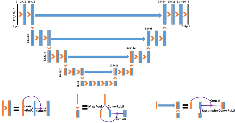
Figure 1 shows the neural network architecture, HD U-net, used in this work. The general HD U-net structure was proposed for three-dimensional dose prediction for head and neck cancer patients.⁹ We adopted the main neural network operations of the original HD U-net and made modifications to the architecture. Patient’s CT image and corresponding RT dose distribution are used as model inputs and the CS dose distribution is the output. As can be seen in Figure 1, the HD U-net contains five levels to reduce the feature size from 128×128×16 down to 8×8×1, where 2×2×2 max pooling was performed between layers. The convolutional kernel of size 3×3×3 was implemented during convolution with zero padding to maintain the feature size. Sixteen feature maps were used in each convolutional step on the left half of the network. On the right half of the network, the number of filters increased by 16 for each level from the bottom to the top. The convolution and rectified linear unit (ReLU) operations were followed by batch normalization (BN) in the HD U-net, as suggested for dose prediction with U-net.⁷ Because we observed no overfitting issue, we kept the dropout rate at 0. The learning rate was carefully adjusted to 10⁻⁴, and the Adam algorithm¹⁴ was selected as the optimizer to minimize the loss function of the mean squared error (MSE). The deep learning model was built and implemented in Keras with Tensorflow¹⁵ as the back end.

Figure 1.

Schematic of the HD U-net architecture used for the dose calculation. The number above the boxes represents the number of concatenated features, and those to the left show the size of the three-dimensional feature maps.⁹ The model inputs are the patient’s CT image and corresponding RT dose distribution while the output is the CS dose distribution.

2.2. Patient data

We used 78 prostate IMRT patients in this feasibility study. For each patient, the treatment plan with seven 6-MV photon beams was re-calculated using both RT and CS algorithms. The input and output volume dimensions were 256×256×64 for 77 patients and 256×256×62 for the remaining one patient.

2.3. Training and evaluation

Seventy patients were randomly assigned as the training data, and the remaining eight patients were held aside as separate testing data. A five-fold cross-validation was performed during the training stage to assess the performance stability and variability of the proposed HD U-net model. The 70 patients were divided into 5 folds with 14 patients in each fold. For every training round, four folds (56 patients) were used for training, and the last fold was reserved for validation. The weights were randomly initialized for each round and then updated based on its training dataset. The five-fold training results were collected and assessed to ensure stability of the DL architecture. A final model was trained on the 5-fold patients combined, that is total of 70 patients. The final model was then tested on the other eight patients.

During each training iteration, a patch of size 128×128×16 was randomly selected from the patient CT and dose images. This training-by-patch method, similar to data augmentation, could reduce overfitting and allow us to use a small training dataset (70 patients). The number of epochs, with around 56 iterations in each epoch, was optimized through fine tuning and determined to be 300.

For the eight testing cases, we computed the global gamma passing rate at 1mm/1% and 2mm/2% for the assessment. We also analyzed the statistics, including the mean, standard deviation, minimum, and maximum of the differences between CS and DL dose distributions for various IMRT clinical evaluation criteria (key dose-volume points). We also calculated the dose volume histogram (DVH) comparison of CS, RT, and DL dose distributions for testing patients. In addition, we computed the error histograms for critical regions.

The DL model was trained on NVIDIA Tesla K80 dual-GPU cards with 12 GB dedicated RAM. The evaluation on testing patients was performed on one NVIDIA Tesla V100 GPU card with 32 GB dedicated RAM.

3. Results

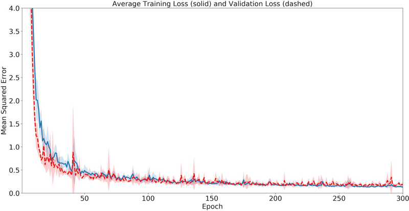
Figure 2 displays the training and validation losses for the HD U-net. Generally, both the training and validation losses decrease as the epoch increases. Based on all five validation losses, we observed no over-fitting issue.

Figure 2.

The average loss across the 5 cross-validation folds, where the solid line represents the training loss and the dashed line shows the validation loss.

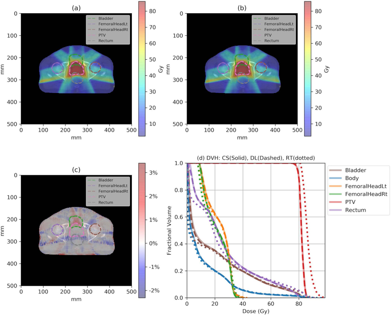
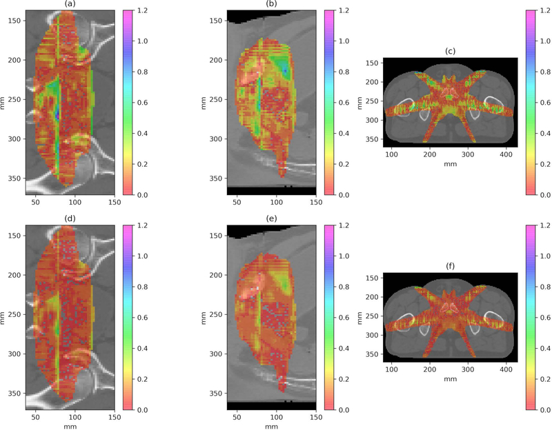
The trained model was applied to calculate the eight testing plans, and the average calculation time was 1.19 seconds with a standard deviation of 0.01 seconds. Figure 3 illustrates the CS dose (a), the DL dose (b) and their difference (c) distributions loaded on the CT slice for an example patient. As can be seen, the DL dose is very close to the CS dose, with a difference of less than ~2% of the prescription dose. Figure 3 (d) shows the DVH curves for the same patient. The solid lines represent the CS dose, while the dashed lines and the dotted lines represent the DL and RT doses, respectively. One can see that the DL DVH curves (dashed) are mostly covered by the CS DVH curves (solid) in Figure 3 (d), indicating a clinically acceptable accuracy for the DL dose and a considerable improvement from the RT dose. Figure 4 shows the coronal, sagittal, and axial planes of global gamma index maps at 1mm/1% criteria (a), (b), (c) and 2mm/2% criteria (d), (e), (f) with the threshold of 20% maximum dose for one example test patient. The overall gamma passing rate is further summarized in Table 1.

Figure 3.

(a) One slice of the CS dose distribution; (b) the corresponding slice of the DL dose distribution; (c) the relative dose difference ($\frac{D_{DL}-D_{CS}}{D_{Rx}}$) distribution; and (d) the DVH plots of the CS (solid), the DL (dashed), and the RT (dotted) doses for one example test patient. Note that CS and DL DVH curves completely overlap with each other.

Figure 4.

The coronal, sagittal, and axial planes of gamma index maps at 1mm/1% criteria (a), (b), (c) and 2mm/2% criteria (d), (e), (f) for one example test patient.

Table 1.

The Gamma passing rate of DL dose calculation for the eight testing patients.

Gamma Index
Criterion		1mm/1%	2mm/2%
Patient	1	99.1%	100%
	2	99.9%	100%
	3	97.6%	100%
	4	99.8%	100%
	5	99.9%	100%
	6	99.9%	100%
	7	95.7%	99.7%
	8	96.3%	99.8%
	Mean	98.5%	99.9%
	SD	1.6%	0.1%

Table 1 shows the global gamma passing rates at 1mm/1% and 2mm/2% criteria for the DL doses for the eight testing patients, using the CS dose as the reference. As can be seen, the gamma analysis indicates the high accuracy of the DL dose in both settings. The gamma passing rate for the 1mm/1% criterion is as high as 98.50% on average with a standard deviation of 1.6%. For the 2mm/2% criterion, the corresponding numbers become 99.9% and 0.10%. These numbers indicate that there is essentially no clinically meaningful difference between DL and CS dose distributions. Table 2 displays the mean, standard deviation, min, and max of the difference in clinical evaluation criteria between CS and DL dose calculations. The differences of DL and CS algorithms in the D₉₅ of PTV for the eight testing patients fall between −1.38 Gy and 0.66 Gy where the average difference is −0.25 Gy. For the percent volume difference at various dose levels for rectum (75 Gy, 70 Gy, 65 Gy, 45 Gy), bladder (80 Gy, 75 Gy, 70 Gy, 65 Gy), and femoral heads (50 Gy), the mean values are within ±0.16%, the standard deviations are less than 0.35%. The difference in mean dose for femoral heads is also negligibly small. All of these numbers indicate that the two dose distributions computed by DL and CS are clinically identical.

Table 2.

The mean, standard deviation, min, and max of the difference (DL-CS) in clinical evaluation criteria between DL and CS dose calculations for the eight testing patients. The volume differences are in percent volume and the dose differences are in Gy.

		Mean	SD	Min	Max
PTV	D95	−0.25	0.67	−1.38	0.66
Rectum	V75	−0.16%	0.32%	−0.78%	0.27%
	V70	−0.16%	0.35%	−0.97%	0.10%
	V65	−0.09%	0.20%	−0.46%	0.14%
	V45	−0.13%	0.13%	−0.33%	0.08%
Bladder	V80	0.02%	0.26%	−0.44%	0.40%
	V75	0.04%	0.10%	−0.12%	0.18%
	V70	0.04%	0.12%	−0.08%	0.21%
	V65	0.01%	0.12%	−0.16%	0.16%
Femoral Heads	Dmean	−0.02	0.13	−0.24	0.12
	V50	0.00%	0.00%	0.00%	0.00%

4. Discussion and Conclusions

As discussed in Section 1, there is a dilemma between efficiency and accuracy for all existing dose calculation engines. In this study, we focus on the feasibility of using DL to boost an inaccurate dose distribution to an accurate one. Our model by no means has been optimized for efficiency but it is quite fast (about one second for a prostate IMRT plan dose calculation). We expect an even higher efficiency through model optimization which will be our future work. Also, we used CS calculation as the model output simply because it is accurate enough and easy to implement. However, our final goal is to achieve Monte Carlo calculation accuracy with real time efficiency using DL models. Then it makes more sense to study the speed-up factor versus Monte Carlo simulation in our future work.

This paper, using prostate IMRT cases, is simply to show the feasibility of using DL as a new dose calculation method. We do not intend to present a full dose calculation system and we have not tested the model for various tumor sites, treatment machines, beam energies, treatment techniques, etc. Those will also be our next step along this research direction.

As a general problem for any applications of DL in medicine, DL models tend to fail for unseen scenarios such as infrequent anatomies. However, the severity of the problem for our proposed method seems to be low since the model input is the RT dose which has taken into account the major physical law (primary beam attenuation) and DL is only used to learn the difference between RT and CS doses. Therefore, we do not expect any crazy outcome, such as a dose distribution with a hollow sphere. Still, this problem needs to be addressed carefully. One way is to make the training dataset as comprehensive as possible, including all clinically relevant cases such as patients with hip prosthetic. Otherwise the model can produce unreasonable results for cases not seen in the training dataset. The second thing to do is, when implementing a DL model for the clinical use, we have to take a careful and gradual step-by-step approach. For example, for the proposed DL-based dose engine, we probably should use it as a secondary dose check algorithm first, rather than a primary dose engine on day one.

To our knowledge, this is the first instance of successful dose calculation for radiotherapy using deep learning. Our work shows that deep learning-based methods may be able to achieve a high dose calculation accuracy with a high efficiency, which may play an important role for real-time adaptive radiation therapy. Also, since the deep learning-based methods are completely different from the existing measurement-based or model-based methods, they are well suited for secondary dose verification.

References

- 1.Ahnesjo A, Aspradakis MM. Dose calculations for external photon beams in radiotherapy. Phys Med Biol. 1999;44(11):R99–R155. [DOI] [PubMed] [Google Scholar]
- 2.Luong M-T, Pham H, Manning CD. Effective approaches to attention-based neural machine translation. arXiv preprint. 2015;arXiv:1508.04025. [Google Scholar]
- 3.Lee J, Cho K, Hofmann T. Fully character-level neural machine translation without explicit segmentation. arXiv preprint. 2017;arXiv:1610.03017. [Google Scholar]
- 4.Simonyan K, Zisserman A. Very deep convolutional networks for large-scale image recognition. arXiv preprint. 2014;arXiv:1409.1556. [Google Scholar]
- 5.He K, Zhang X, Ren S, Sun J. Deep residual learning for image recognition. arXiv preprint. 2015;arXiv:1512.03385. [Google Scholar]
- 6.Ronneberger O, Fischer P, Brox T. U-Net: convolutional networks for biomedical image segmentation. Medical Image Computing and Computer-Assisted Intervention – MICCAI 2015 Lecture Notes in Computer Science. 2015;9351:234–241. [Google Scholar]
- 7.Nguyen D, Long T, Jia X, et al. Dose prediction with U-net: a feasibility study for predicting dose distributions from contours using deep learning on prostate IMRT patients. arXiv preprint. 2017;arXiv:1709.09233. Scientific Reports. 2019;9(1):1076. [DOI] [PMC free article] [PubMed] [Google Scholar]
- 8.Barragan-Montero AM, Nguyen D, Lu W, et al. Three-dimensional dose prediction for lung IMRT patients with deep neural networks: robust learning from heterogeneous beam configurations. arXiv preprint. 2018;arXiv:1812.06934. [DOI] [PubMed] [Google Scholar]
- 9.Nguyen D, Jia X, Sher D, et al. 3D radiotherapy dose prediction on head and neck cancer patients with a hierarchically densely connected U-net deep learning architecture. arXiv preprint. 2018; arXiv:1805.10397. Phys Med Biol 2019;64(6). [DOI] [PubMed] [Google Scholar]
- 10.Lu W, Chen M. Fluence-convolution broad-beam (FCBB) dose calculation. Phys Med Biol. 2010;55(23):7211–7229. [DOI] [PubMed] [Google Scholar]
- 11.Ahnesjo A Collapsed cone Convolution of radiant energy for photon dose calculation in heterogeneous media. Med Phys. 1989;16(4):577–592. [DOI] [PubMed] [Google Scholar]
- 12.Ulmer W, Kaissl W. The inverse problem of a Gaussian convolution and its application to the finite size of the measurement chambers/detectors in photon and proton dosimetry. Phys Med Biol. 2003;48(6):707–727. [DOI] [PubMed] [Google Scholar]
- 13.Ulmer W, Pyyry J, Kaissl W. A 3D photon superposition/convolution algorithm and its foundation on results of Monte Carlo calculations. Phys Med Biol. 2005;50(8):1767–1790. [DOI] [PubMed] [Google Scholar]
- 14.Kingma DP, Ba J. Adam: A method for stochastic optimization. arXiv preprint. 2014;arXiv:1412.6980. [Google Scholar]
- 15.Abadi M, Agarwal A, Barham P, et al. Tensorflow: Large-scale machine learning on heterogeneous distributed systems. arXiv preprint. 2016; arXiv:1603.04467. [Google Scholar]