Abstract
Background: Mathematical modeling of vector-borne diseases and forecasting of epidemics outbreak are global challenges and big point of concern worldwide. The outbreaks depend on different social and demographic factors based on human mobility structured with the help of mathematical models for vector-borne disease transmission. In Dec 2019, an infectious disease is known as “coronavirus” (officially declared as COVID-19 by WHO) emerged in Wuhan (Capital city of Hubei, China) and spread quickly to all over the china with over 50,000 cases including more than 1000 death within a short period of one month. Multimodal modeling of robust dynamics system is a complex, challenging and fast growing area of the research.
Objectives: The main objective of this proposed hybrid computing technique are as follows: The innovative design of the NAR-RBFs neural network paradigm is designed to construct the SITR epidemic differential equation (DE) model to ascertain the different features of the spread of COVID-19. The new set of transformations is introduced for nonlinear input to achieve with a higher level of accuracy, stability, and convergence analysis.
Methods: Multimodal modeling of robust dynamics system is a complex, challenging and fast growing area of the research. In this research bimodal spread of COVID-19 is investigated with hybrid model based on nonlinear autoregressive with radial base function (NAR-RBFs) neural network for SITR model. Chaotic and stochastic data of the pandemic. A new class of transformation is presented for the system of ordinary differential equation (ODE) for fast convergence and improvement of desired accuracy level. The proposed transformations convert local optimum values to global values before implementation of bimodal paradigm.
Results: This suggested NAR-RBFs model is investigated for the bi-module nature of SITR model with additional feature of fragility in modeling of stochastic variation ability for different cases and scenarios with constraints variation. Best agreement of the proposed bimodal paradigm with outstanding numerical solver is confirmed based on statistical results calculated from MSE, RMSE and MAPE with accuracy level based on mean square error up to 1E-25, which further validates the stability and consistence of bimodal proposed model.
Conclusions: This computational technique is shown extraordinary results in terms of accuracy and convergence. The outcomes of this study will be useful in forecasting the progression of COVID-19, the influence of several deciding parameters overspread of COVID-19 and can help for planning, monitoring as well as preventing the spread of COVID-19.
Keywords: SITR Model, COVID-19 dynamicd, Epidemic model, Neural networks, Radial Base functions
Abbreviations: NAR, Nonlinear Autoregressive; St Dev, Standard Deviation; RBFs, Radial Basic Functions; WHO, World health organization; MSE, Mean Square Error; PDEs, Partial differential equations; ARIMA, Auto-Regressive Integrated Moving; ODEs, Ordinary differential equations Average
1. Introduction
Mathematical modeling of Vector-borne diseases and forecasting of epidemics outbreak are global challenges and big point of concern worldwide. The outbreaks depend on different social and demographic factors based on human mobility which paradigm with mathematical models for vector-borne disease transmission. In Dec 2019, an infectious disease is known as “coronavirus” (officially declared as COVID-19 by WHO) emerged in Wuhan (Capital city of Hubei, China) and spread quickly to all over the china with over 50,000 cases including more than 1000 death within a short period of just one month [1] after the outbreak of the pandemic. To overcome the outbreak massive type of restriction on public gathering, traveling and self-safety like wearing masks with social distancing were implemented. On initial stages, the key symptoms for this disease are fever, flu, and dry cough which might lead to difficulty in breathing, headache, and loss of taste/ smell for its critical cases. Generally, the recovery rate from the pandemic is around 80 ~ 85 % without any special treatment [2,3]. The COVID-19 badly affects older people (almost age of 60 or more), and those who are facing serious medical diseases like cardiovascular disease, diabetes, chronic respiratory and cancer. Those who have a fever, breathing difficulty, and dry cough should pursue medical care. As of 20th December, 2020 more than 76.11 million people have been infected and more than 1.6 million people have died with this virus but 53.83 million persons got recovered from this virus all over the world. Data of the top 10 countries mostly got infected by COVID-19 (WHO sources [4]) has been presented in Table 1 , whereas the graphical trend of the spread of virus has been shown in Fig. 1 .
Table 1.
Country-wise data Infected, Recovered and Died persons for COVID-19 [4] (As on 20 December 2020).
| S No | Country | Total infected | Total Recovered | Total Deaths |
|---|---|---|---|---|
| 1 | USA | 17,888,353 | 10,394,286 | 320,845 |
| 2 | India | 10,005,850 | 9,550,712 | 145,178 |
| 3 | Brazil | 7,163,912 | 6,198,185 | 185,687 |
| 4 | Russia | 2,819,429 | 2,254,742 | 50,347 |
| 5 | France | 2,442,990 | 182,656 | 60,229 |
| 6 | Turkey | 1,982,090 | 1,753,552 | 17,610 |
| 7 | UK | 1,977,167 | 1,244,367 | 66,541 |
| 8 | Italy | 1,921,778 | 1,226,086 | 67,894 |
| 9 | Spain | 1,817,448 | 1,145,871 | 48,926 |
| 10 | Argentina | 1,531,374 | 1,356,755 | 41,672 |
Fig. 1.
Total number of infected and died persons with COVID-19 all over the world [4].
Some researchers studied the basic reproduction number (R0) of COVID-19 and found that it lies in the range of 1.4 - 6.6 which is very high than influenza, Ebola, and SARS epidemics [5]. This disease has a very fast speed of transfer from one person to others through small droplets of coughing or sneezing. The numbers of infected person are hence increasing day by day at a very high rate. At present, there is no vaccine or proper treatment is available for the patients of this disease and in the opinion of medical experts, the only way to reduce its rising trend is to keep the people away from infected persons and try to keep all infected persons in isolation or quarantined to avoid their social contact with healthy persons in the society. The global economy has been badly affected by control measures taken to prevent the spread of COVID-19, however, it is still uncertain whether this type of strategy has which type of effect on the spread of COVID-19. Therefore, it is necessary to measure the influence of all these parameters over epidemic development.
Analysis of data shows that the number of deaths does not only depend on the infected persons, besides this many other factors like weather / environmental conditions, average ages of person, and natural immunity of persons against viral diseases also matters. The rising trend of COVID-19 in different countries are presented in Fig. 2 .
Fig. 2.
Trend of COVID-19 in Different Countries [4].
The average incubation period for this virus is 7 - 14 days and the time required from infection to recovery or death is about 10 days based on several factors [6,7]. Roosa et al. [8] offered three different mathematical models to present the short term estimation of the collective number of cases for COVID-19. Kucharski et al. [9] suggested an SEIR model with some necessary modifications to study the rate of spreading of COVID-19. Yang et al. [10] proposed various SEIR models with employing artificial intelligence schemes to predict the rising trend, epidemic peaks, and sizes of COVID-19 in china. Ivorra et al. [11] developed an innovative θ-SEIHRD model while considering various special characteristics of the disease to estimate the spread of disease with an approximate magnitude of peaks. Later on, the results proposed by this model matches the actual data of COVID-19. All through this battle against an epidemic situation, theoretical research based on the epidemiological model has the same worth and importance as biological and medical studies have. These mathematical models are very helpful in understanding, comparing, and estimating the effect of various parameters (control measure and natural phenomenon) on the spreading and decaying of an epidemic outbreak. These mathematical models have advantages over other stochastic approaches such as less computational complications and involvement of ordinary differential equations provides better analysis for understanding the model. Bonyah et al. [12] numerically investigated the SEIR based epidemic model of Zika virus with constant and dependent control to measure the effect of different parameters on disease spread. Yavuz et al. [13] numerically investigated the schistomosiasis fractional dynamic model by utilizing the Mittag-Leffler and exponential kernals. Furthermore, authors in [14] observed that in cases where determining distribution probability is very difficult, it is better to prefer mathematical modeling over the stochastic approaches. Several studies have been done to describe the epidemic dynamics of COVID-19 in China and elsewhere with the help of several conventional mathematical models [15], [16], [17], [18]. Over time, development in medical treatment, as well as more exact approaches of stochastic and statistical reasoning [19], [20], [21], [22], [23], [24] to study the epidemic behavior have stepped up.
Settati et al. [25] provided computer simulations to explain various theoretical results based on SIRI epidemic model with nonlinear variation. Karimi et al. [26] proposed a hybrid model based on genetic algorithm (GA) and back propagation network (BPN) for the proper assessment of nanofluid density with improved accuracy. Ramírez et al. [27] presented a hybrid model by joining the neural network with fuzzy logic by means of 2-lead for irregular cardiac heartbeat. Wang et al. [28] offered a hybrid model by combining the correction and heuristic intelligent optimization algorithm with outliner detection to predict the air pollution in environment. Gao et al. [29] used a hybrid predictive model built on artificial neural network (ANN) and imperialist competition algorithm (ICA) to analyze the slope stability behavior of unified soils. Cheema et al. [30] presented an intelligent computing solution based on artificial neural networks for the mathematical model of novel COVID-19 by dividing the population into various classes. Wieczorek et al. [31] used neural networks by exploiting the NAdam training model to predict the spread of COVID-19 based on the real value data. Marques et al. [32] proposed an automated medical diagnostic system by utilizing convolutional neural network with using Efficient Net architecture. Khan et al. [33] applied an Auto-Regressive Integrated Moving Average (ARIMA) model on the realistic collected data to predict and forecast the affected cases of COVID-19 in future. Authors then compared the accuracy of results with a NAR based solution and found a high level of accuracy in their results. Umar et al. [34] presented a SITR model representing the dynamics of COVID-19 and then used the modern stochastic intelligent computational methodology based on feed forward artificial neural networks to solve that model to study the variation of various classes on different involved parameters. Jung et al. [35] proposed a SIR model based on different classes to present the dynamics of COVID-19 in South Korea and then used neural network with deep learning to solve the model. Naik et al. [36] numerically investigated a COVID-19 model based on Caputo operator and presented graphical results to envision the effectiveness of introduced arbitrary order derivative. Wang et al. [37] used the latest alpha-Sutte indicator to forecast the rising trend of COVID-19. Authors compare their result with the results of ARIMA method and found alpha-Sutte indicator more efficient and reliable as compared to ARIMA on the basis of root mean square error and absolute percentage error.
Contrary to these statistical techniques [38,39] mathematical modeling based on various differential equations [40], [41], [42] got very less consideration, although these mathematical models can deliver more detailed information for the epidemic dynamics. Conventional SIR model (susceptible-infectious-recovered) is being broadly used for describing epidemic of COVID-19 in all over the world. In this work, spread dynamics of COVID-19 is evaluated by designing innovative SITR epidemic model with the division of susceptible class (S) into two portions and by introducing a new class of treatment (T) to observe the epidemic situation which makes the model of COVID-19 to work with the consideration of continuous treatment of affected persons. Influence of various key parameters over the spreading of COVID-19 has been investigated. Innovative contribution of the design deep learning neural network based on different capabilities are presented in the following salient features: -
-
•
Computational strength of deep learning neural network based on nonlinear autoregressive (NAR) with radial base functions (RBFs) networks enhance the computing power and level of accuracy of the solver technique.
-
•
The hybrid model can pinpoint and capture the global as well as local aspects in the modeling of nonlinear differential equations representing the SITR epidemic model.
-
•
The innovative design of the NAR-RBFs neural network paradigm is designed to model the SITR epidemic differential equation (DE) model with additional term of stochastic variation to ascertain the different features of the spread of COVID-19.
-
•
The new set of transformations are introduced for nonlinear input to achieve with a higher level of accuracy, stability, and convergence analysis.
Rest of the paper is organized as follows: -
Detailed mathematical modeling of the SITR model has been presented in Section 2. Solution methodology of the suggested model has been briefly described in section 3. Statistical analysis of the all involved variables of SITR model is investigated in section 4. In Section 5 explanation of NAR-RBFs network structure is presented. Detailed numerical and graphical result with discussion are presented in section 6. A comparative study for alternate SIR model has been presented in Section 7 and at last section 8 consist of conclusion of the research.
2. Mathematical formulation of the model
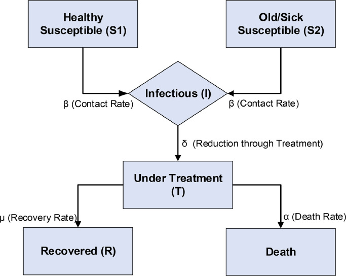
In this section, a general SITR model along with description of basic characteristics of the model is presented. A detailed structure of the SITR model with the contribution of several parameters is shown in Fig. 3 . These type of mathematical models based on various types of differential equations often gives detailed necessary information regarding the dynamics of an epidemic situation.
Fig. 3.
Epidemic model (SITR) for COVID-19 dynamics including φ(t)in all four classes.
Basic Characteristics of the Model:-
-
(1)
Susceptible class S1 (t):- This class includes those persons who are not yet infected with the virus.
-
(2)
Susceptible class S2 (t):- This class also represents that persons which are not yet been infected with the virus, but persons in this class have some types of sickness/illness or they are of an older age which creates greater chances for these persons to get infected by virus then class S1.
-
(3)
Infectious class I (t):- This class includes those persons who are infected by Covid-19 and they can further transmit the virus to other healthy persons.
-
(4)
Treatment Class T (t):- Persons in this class or either under the hospital treatment or in the state of quarantined. These persons can either move to recovered class by recovery or can die from the virus.
-
(5)
Recovered class R (t):- This class includes those persons who were previously got infected from the virus and either survived or got recovered with treatment.
Mathematical Model:-
Under those assumptions, the proposed SITR model [43] can be described in term of following ordinary differential equations:-
| (1) |
| (2) |
| (3) |
| (4) |
| (5) |
With initial boundary conditions
| (6) |
Assigned values for various parameters involved in equations (1~5) has been mentioned in Table 2 . Whereas, ϕ(t) in the equations (1 ~ 5) represents the abrupt change due to different factors including social gathering, huge travelling and public interaction at different level, that can produce any sudden rise in the number of susceptible/infectious persons. It is pertinent to highlight that recovery rate μ and death rate α can also be treated as time-dependent parameters since the recovery rate increase certainly decreases the death rate over time with proper medical treatments, an invention of vaccine or drugs and isolation of infected persons from the society. In the mathematical model, the effectiveness of increasing recovery rate and decreasing death rate over the number of susceptible, infectious, and recovered persons is studied. The behavior of other important parameters with their variation and its impact on recovery rate is calculated and modeled. Different studied are presented to study the relationships between environmental conditions (temperature, humidity, etc.) and the spread of COVID-19. Luo et al. [44] observed that the spreading behavior of COVID-19 is not following the hypothesis that higher values of humidity bound the transmission and existence of viruses. Whereas, Wang et al. [45] find that the increase in temperature corresponds to less transmission rate and shorter survival period of the virus outside the host. Therefore, without any scientific proof regarding the influence of temperature and humidity on the spreading of COVID-19, these factors are not considered in proposed model.
Table 2.
Description and values for various involved parameters in SITR model.
| Symbol | Parameter Description | Assigned Value |
|---|---|---|
| β | Contact rate | 0.3 |
| B | Natural birth rate | 0.3 |
| δ | Reduce infection from the treatment | 0.3 |
| σ | Fever, tiredness and dry cough rate | 0.005 |
| μ | Recovery rate | 0.1 |
| α | Death rate | 0.25 |
| ρ | Rate of infection from the treatment | 0.3 |
| ψ | Healthy food rate | 0.2 |
| ε | Sleep rate | 0.1 |
3. Solution methodology
NAR network based on sigmoid function performs globally [46] whereas the radial based network function deals to treat the local behavior of inputs. With the variation of input based on time interval from the center towards radii, radial displacement governed by neurons reduces which transform most of the RBF function to their zero states, however with the increase in input data sigmoid function stay close to 1. These specific characteristics enable the combination of RBF with Sigmoid function to deal simultaneously with local as well as global features of modeling.
4. Non-linear autoregressive neural network (NAR)
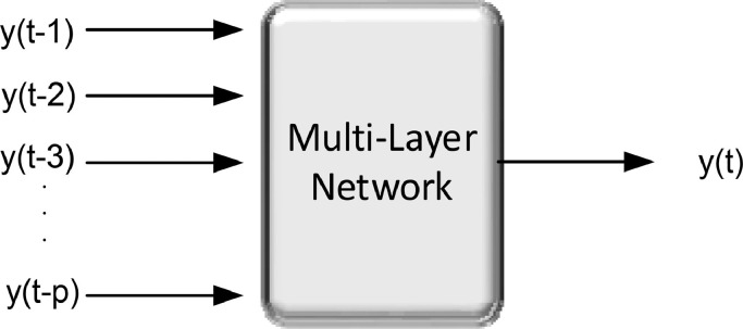
A maximum number of time series models are based on temporary periods and high variations, which makes them difficult to model through linear modeling therefore a non-linear attitude is proposed. Fig. 4 shows a nonlinear auto aggressive neural network (NAR) [47] is a discrete model containing three different layers (input, hidden and output) with two delay steps (input and output) is being used for the prediction of non-linear time series, which can be expressed as [48]:-
Fig. 4.
Non-Linear Autoregressive Neural Network (NAR).
Through the above mathematical relation, it is easy to judge that how by using the previous p values of the series, NAR neural network is utilized to forecast the values any output y(t) at any point t. The unknown function h(*) is being approximated with the training of neural networks through optimizing the neural weight and number of neurons. The term at the end is an approximate error of the complete seriesy(t).
The number of neurons and hidden layers are adjustable and can be optimized through hit and trial basis depending upon the accuracy and performance of the system. It should be kept in mind that a higher number of neurons will result in better accuracy of the computation but it also makes the system more complicated to solve, whereas the lower number of neurons may limit the computing capabilities of the network. The most widely and commonly used rule for NAR neural network is the Levenberg-Marquardt technique [49,50].
NAR neural network uses the mean square error (MSE) error sum of squares (SSE) to show the accuracy and reliability of the computations. Whereas, yi are the values of ith data set, is the value of similar data set obtained through network operation and k is the number of data set provided to the neural network for its operation.
5. Radial base function (RBF)
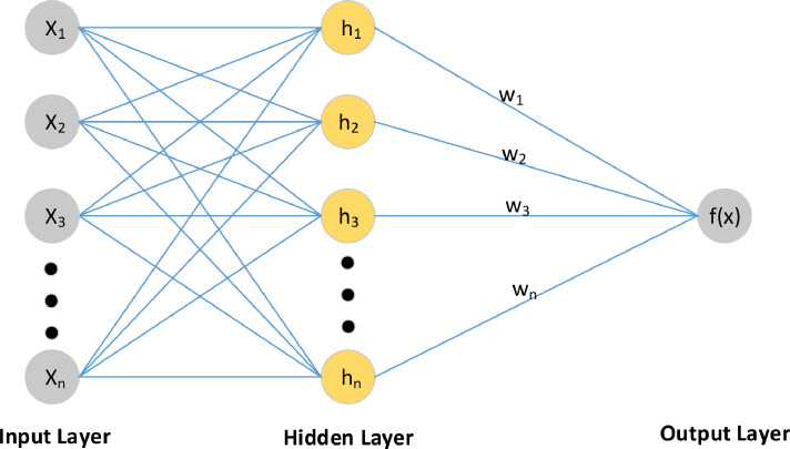
Most basic Radial basis function (RBF) operates on followings three layers with each layer having its task that is completely different from the other two:-
-
•
Input layer: - This first layer is constructed by source nodes that join the network with its environment.
-
•
Hidden layer: - This second layer has the role of application of nonlinear transformation from the input layer to the hidden layer.
-
•
Output layer: - This third layer is linear and an arrangement of hidden functions. It has the role to supply the reaction of a network to the stimulation array given to input layer.
Structure of RBFs network has been shown in Fig. 5 . The basic linear model for function f(x) can be written as
Fig. 5.
Structure of RBF Network.
The f (.) can be expressed as a linear combination of ‘m’ basis functions, whereas, h(x) normally represents the Gaussian function.
Whereas, c is the center and r is the radius.
6. Statistical analysis of data
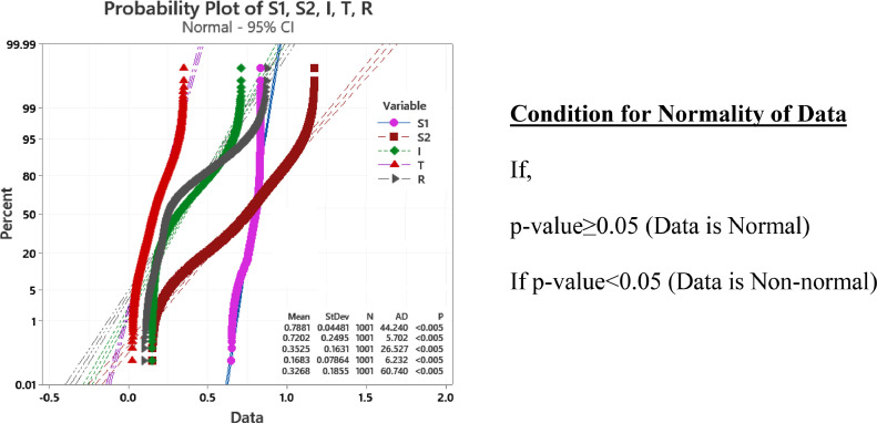
In problems governed by the system of differential equations, linear input between a fixed domain is used very often in many types of machine learning techniques by neglecting the non-linear behavior of outputs. In Fig. 6 , the probability distribution curves of the outputs (S1, S2, I, T, R) shows their strong non-linear behavior. Here the p-value for all outputs is less than 0.005 which is ten times shorter than the minimum range for normal data. So our each of the outputs is strictly non-normal. So the use of linear input in this type of computational process not only makes the process more complicated but also decreases the accuracy of the stochastic process.
Fig. 6.
Probability Plots of data sets of all outputs.
Various types of statistical data in respect of each output in place in Table 3 , which also shows the non-linear distribution of the output data sets. Values of mean with maximum and minimum values tell the distribution of data. The values of Skewness also explain the placement of data from its mean position either in the left or right direction. Additionally, the values of kurtosis give the tail distribution of data from the mean position.
Table 3.
Descriptive Statistics of all classes.
| Variable | Mean | St. Dev. | Variance | Min | Median | Max | Range | Skewness | Kurtosis |
|---|---|---|---|---|---|---|---|---|---|
| S1 | 0.78815 | 0.04481 | 0.00201 | 0.65000 | 0.80203 | 0.83219 | 0.18219 | -1.24 | 0.85 |
| S2 | 0.72021 | 0.24955 | 0.06227 | 0.15000 | 0.74967 | 1.17284 | 1.02284 | -0.35 | -0.61 |
| I | 0.35246 | 0.16313 | 0.02661 | 0.15000 | 0.31232 | 0.71501 | 0.56501 | 0.59 | -0.86 |
| T | 0.16826 | 0.07864 | 0.00618 | 0.02632 | 0.15830 | 0.35000 | 0.32368 | 0.38 | -0.58 |
| R | 0.32684 | 0.18550 | 0.03441 | 0.10000 | 0.24670 | 0.87314 | 0.77314 | 1.27 | 0.66 |
6.1. Introduction of non-linear transformation
Fig. 7(a ~ d) shows the multiple nature of outputs with various type of statistical data placed against each plot. Here instead of using simple linear input against each output with different characteristics and behavior, a special transformation for input as per corresponding output is introduced. This type of transformation helps the computational process to ensure the conversion of linear input into bi-module input or as per output requirements. Therefore, in the suggested approach, a set of transformations are presented to reduce the local optimum to global optimum. In the first step, this transformation converts the linear input into the desired bi-module greater input with ensuring its convergence before being used in the machine learning process. Table 4 shows the set of transformations to achieve the desired nature of transmuted inputs.
Fig. 7.
Graphical view of outputs.
Table 4.
Proposed transformations to achieve desired outputs.
| Required Nature | Transformation to be Used | Resultant Nature |
|---|---|---|
| Highly stochastic, Nonlinear bi-model | T = t4 − t−4T = t4 + t−4 | Bi-module |
7. Hybrid NAR-RBF methodology
Our proposed NAR-RBF model can be expressed as
Here, Ni(x) represents the non-linear neural networks working under the methodology of NAR which used Gaussian transfer function and model the global features whereas, Li(x) shows the data modeling with radial basis function (RBF) which deals very well with the local trend of the model. Structure of proposed NAR-RBFs neural network has been shown in Fig. 8 . Therefore, by using NAR and RBF, this hybrid model simultaneously entertains the global and local features of the non-linear database outputs.
Fig 8.
Structure of Proposed NAR-RBFs Model.
8. Results of NAR and NAR-RBFs networks
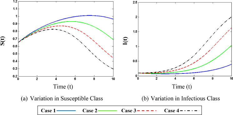
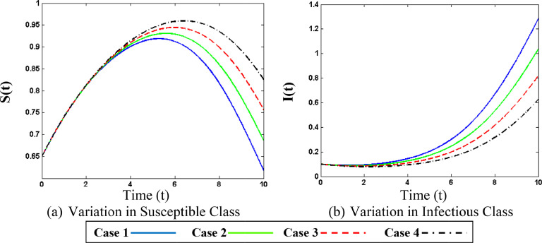
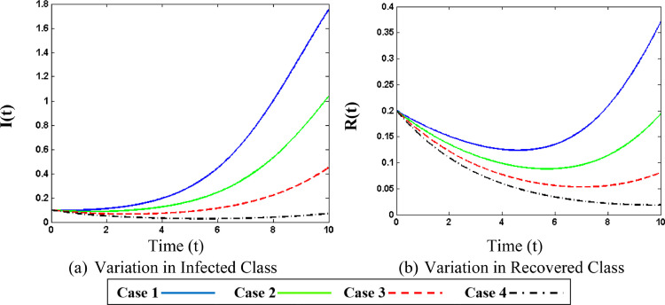
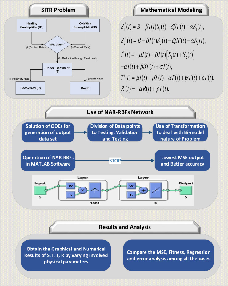
The system of differential equations (1~5) representing the SITR model with initial boundary conditions in (6) for each case of all scenarios are solved separately with the help of NDSolve in Mathematica by employing the RK technique. Table 5 represents the variation in important parameters to get their plots of variation against the number of susceptible, infectious, and recovered persons. Complete process in the form of graphical abstract is being presented in Fig. 9 . The impact of variation of different important parameters on the epidemic curves are represented in Figs. 11, 13 and 15.
Table 5.
Variation of different involved parameters.
| Scenarios | Variable Parameter | Case I | Case II | Case III | Case IV |
|---|---|---|---|---|---|
| 1 | Contact Rate | β=0.25 | β=0.30 | β=0.35 | β=0.40 |
| 2 | Recovery Rate | μ=0.08 | μ=0.10 | μ=0.12 | μ=0.14 |
| 3 | Death Rate | α=0.20 | α=0.25 | α=0.30 | α=0.35 |
Fig. 9.
Structure of Proposed NAR-RBFs Model.
Fig. 11.
Influence of contact rate on various classes.
Fig. 13.
Influence of Recovery Rate on various classes.
Fig. 15.
Influence of Death Rate on various classes.
Output (in the form of data sets) against unique input is being exported to MATLAB for use in a supervised neural network. Total 1001 data set point are created between 0 and 10 by keeping the step size of 0.01 for each variable (S1(t), S2 (t), I(t), T(t), R(t)), out of total imported data set points 90% of the points are selected for training whereas 5% of the points are being selected for validation and testing each. The number of neurons is also adjusted in the range of 80 to 100 according to the desired accuracy of the computational results. The basic structure of the neural network for five outputs against one input is being shown in Fig. 10 .
Fig. 10.
Hidden structure of NAR network.
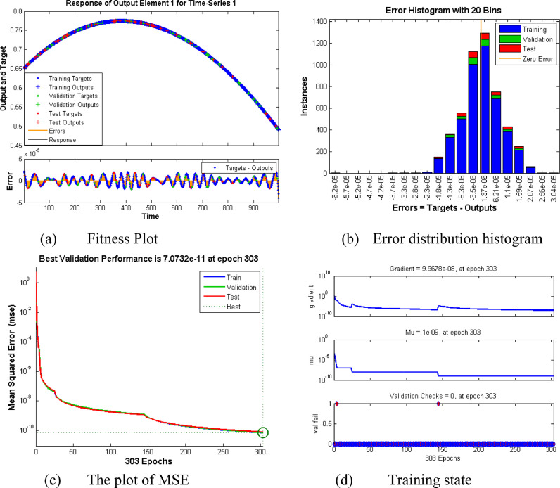
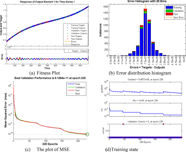
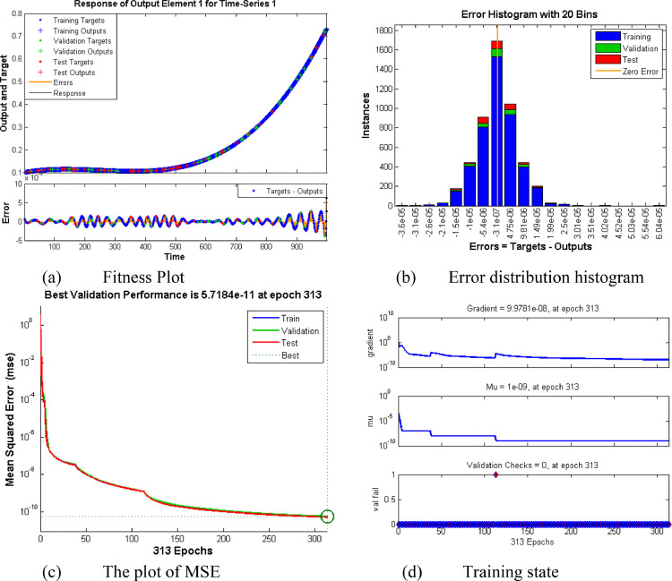
Data set containing 1001 points for each output is solved with a supervised neural network as per four cases of three different scenarios as per Table 5. Performance and accuracy analysis of the method is being given graphically in Figs. 12, 14 and 16. Comparison of all computational and statistical data containing the values of performance, gradient, Mu, epochs, number of hidden neurons, and MSE for Training, Testing & Validation for all cases of each scenario are displayed in Table 6 .
Fig. 12.
Graphical view of the various plot of Scenario 1 (NAR).
Fig. 14.
Graphical view of the various plot of Scenario 1I (NAR).
Fig. 16.
Graphical view of the various plot of Scenario 1II (NAR).
Table 6.
Complete numerical analysis of NAR network for SITR model.
| Scen. | Cases | Hidden Neurons | MSE |
Performance | Grad | Mu | Epochs | ||
|---|---|---|---|---|---|---|---|---|---|
| Training | Testing | Validation | |||||||
| (1) Variation in contact Rate | I | 80 | 1.6416e-10 | 2.0375e-10 | 2.0391e-10 | 2.0391e-10 | 9.8096e-08 | 1e-09 | 238 |
| II | 80 | 1.2960e-10 | 1.3412e-10 | 1.3864e-10 | 1.3864e-10 | 9.8835e-08 | 1e-09 | 170 | |
| III | 100 | 6.9596e-11 | 7.9382e-11 | 7.0731e-11 | 7.0732e-11 | 9.9678e-08 | 1e-09 | 303 | |
| IV | 80 | 1.3170e-10 | 1.4411e-10 | 1.6391e-10 | 1.6392e-10 | 9.9336e-08 | 1e-09 | 237 | |
| (1I) Variation in Recovery Rate | I | 100 | 8.6235e-11 | 8.9825e-11 | 8.1883e-11 | 8.1884e-11 | 9.9664e-08 | 1e-09 | 228 |
| II | 100 | 1.2707e-10 | 1.2909e-10 | 1.1492e-10 | 1.1492e-10 | 9.4877e-08 | 1e-09 | 238 | |
| III | 100 | 4.3659e-11 | 4.8787e-11 | 4.7380e-11 | 4.7381e-11 | 9.8947e-08 | 1e-09 | 287 | |
| IV | 100 | 8.7865e-11 | 1.0819e-10 | 1.2749e-10 | 1.2749e-10 | 9.8417e-08 | 1e-09 | 235 | |
| (1II) Variation inDeath Rate | I | 100 | 1.2465e-10 | 1.3521e-10 | 1.4061e-10 | 1.4062e-10 | 9.9688e-08 | 1e-09 | 225 |
| II | 100 | 1.0195e-10 | 1.8944e-10 | 1.2346e-10 | 1.22347e-10 | 9.8326e-08 | 1e-09 | 230 | |
| III | 100 | 7.8275e-11 | 9.8669e-11 | 8.0558e-11 | 8.0558e-10 | 9.7976e-08 | 1e-09 | 250 | |
| IV | 100 | 5.3931e-11 | 5.1339e-11 | 5.7184e-11 | 5.7184e-11 | 9.9781e-08 | 1e-09 | 313 | |
Fig. 11(a) shows that as the rate of contact increases the number of susceptible persons initially rises but after some time it shows a decline. This is because with the higher contact rate more and more persons get infected and moves to infected class therefore the number of people in susceptible class decreases. From Fig. 11(b) increase in the rate of infected persons can be seen with the increase in contact rate. It can be seen that less contact rate results in a mild rise in infected persons while an increase in contact rate will sharply raise the infected persons, which is due to the fact that corona virus has a very fast rate of transfer from one person to others through social gathering with small droplets of coughing or sneezing. Fig. 13(a) exhibits the rising behavior of susceptible persons with higher values of recovery rate. Fig. 13(b) shows that as the recovery rate rises the persons in the infectious class rise slowly. It is understood that when the recovery rate is low then fewer persons will recover from the virus, indeed many of the infected persons will die from the virus. Fig. 15(a) displays the changing behavior of infected persons with various death rates. It is obvious that increasing the death rate will result in reduction of infected persons as more and more persons from infected class moves to death class. Fig. 15(b) shows the variation of recovered persons with different values of the death rate. It can be seen in the plots that with high death rate the number of recovered persons very sharply. This is because when the death rate is high then a large number of persons from infected and recovered class dies which results in the reduction of persons in all of these classes. As the death rate becomes very high the infectious and recovered persons approximately vanish.
Subfigures (12a, 14a, and 16a) exhibits the fitness plots showing the error i.e. the difference between target and output for training, testing, and validation at each point of the input for scenarios 1, 2 and 3 respectively. Similarly, subfigures (12b, 14b, and 16b) shows the distribution of error from the zero error line with the help of error histogram place aside the fitness plots. Accuracy and validity of the process can be judged through the number of values lies close to zero lines. Subfigures (12c, 14c, and 16c) depicts the performance analysis of the computations in term of mean square error (MSE) for Scenario 1, 2, and 3 respectively. The smaller value of MSE indicates the better accuracy and performance of solution methodology. It is being noted that Scenario 3 has a better performance among all others because mean square error (MSE) is minimum (i.e. 5.7184e -11 at 313 epochs) as compared to all other scenarios. Subfigures (12d, 14d, and 16d) shows the plots for gradient, Mu, and validation checks for scenario 1, 2, and 3 respectively. The Gradient is finding another vector during training at each epoch while Mu is the step size of the applied algorithm and validation checks show the generalization measure of the system. It can be seen that smaller the value of Mu leads to better convergence of results.
Comparison results of three different samples of infected I (t) output by the variance of analysis and Tukey simulation test have been carried out, and results are shown in Tables 7 -9 ). Achieved results of F=0 < α with a P-value of 1 with an accuracy of 99.99. As it can be seen through results that each set of output have equal mean which indicates the stability of result and convergence of computational model.
Table 8.
Means and Grouping Information (Tukey Method and 95% Confidence).
| Factor | N | Mean | St Dev. | Grouping | 99% CI |
|---|---|---|---|---|---|
| Infected (1) | 910 | 0.75303 | 0.24331 | A | (0.73224, 0.77382) |
| Infected (2) | 910 | 0.75303 | 0.24330 | A | (0.73224, 0.77382) |
| Infected (3) | 910 | 0.75303 | 0.24330 | A | (0.73224, 0.77382) |
Table 7.
Analysis of Variance (One Way ANOVA).
| Source | DF | Seq. SS | Contribution | Adj SS | F-Value | P-Value |
|---|---|---|---|---|---|---|
| avbFactor | 2 | 0.000 | 0.00% | 0.000 | 0.00 | 1.000 |
| Error | 2727 | 161.431 | 100.00% | 161.431 | ||
| Total | 2729 | 161.431 | 100.00% |
Table 9.
Tukey simultaneous tests for differences of means.
| Difference of Levels | Difference of Means | SE of Difference | 95% CI | T-Value | Adjusted P-Value |
|---|---|---|---|---|---|
| Infected (2) - Infected (1) | -0.0000 | 0.0114 | (-0.0267, 0.0267) | -0.00 | 1.000 |
| Infected (3) - Infected (1) | 0.0000 | 0.0114 | (-0.0267, 0.0267) | 0.00 | 1.000 |
| Infected (3) - Infected (2) | 0.0000 | 0.0114 | (-0.0267, 0.0267) | 0.00 | 1.000 |
Method
Null Hypothesis: All means are equal
Alternate Hypothesis: All means are not equal
Level of Significance: α = 0.01
Comparison for accuracy of proposed model with NAR and RBFs model in term of mean square error (MSE) for each output variable during “Case2 of Scenario 1” are being presented in Appendix Section Table A1 and Table A2 . Same values through NAR-RBFs network along with the values of MSE at different points of the domain for “Case 1 of Scenario 3” is presented in Appendix Section Table A3 . It can be seen that by applying the radial base network on the residual result of NAR the accuracy in terms of MSE up to 2.77E-24 has been achieved.
Table A1.
Numerical Results of NAR & RBFs Based Model for all Variable in SITR Model (Scenario-1, Case-2).
| Input | Value of Target Output |
MSE of NAR Based Model |
MSE of RBFs Based Model |
||||||||||||
|---|---|---|---|---|---|---|---|---|---|---|---|---|---|---|---|
| t | S1(t) | S2(t) | I(t) | T(t) | R(t) | S1(t) | S2(t) | I(t) | T(t) | R(t) | S1(t) | S2(t) | I(t) | T(t) | R(t) |
| 0.5 | 0.68602 | 0.254858 | 0.158557 | 0.316124 | 0.135108 | 2.65E-14 | 5.25E-14 | 1.96E-14 | 1.75E-14 | 1.69E-14 | 9.48e-15 | 1.86e-14 | 7.10e-15 | 6.21e-15 | 5.83e-15 |
| 1.0 | 0.717491 | 0.346206 | 0.168534 | 0.286664 | 0.161638 | 1.68E-14 | 3.23E-14 | 1.39E-14 | 1.10E-14 | 1.27E-14 | 2.74e-15 | 5.61e-15 | 1.98e-15 | 1.77e-15 | 1.64e-15 |
| 1.5 | 0.744643 | 0.42544 | 0.18003 | 0.261169 | 0.181198 | 3.90E-16 | 8.93E-16 | 2.31E-16 | 2.98E-16 | 1.83E-16 | 5.03e-18 | 6.84e-20 | 2.42e-18 | 2.90e-19 | 4.36e-18 |
| 2.0 | 0.767688 | 0.493859 | 0.193155 | 0.239214 | 0.195267 | 1.77E-15 | 3.05E-15 | 1.78E-15 | 1.28E-15 | 1.83E-14 | 5.33e-16 | 1.01e-15 | 3.63e-16 | 3.33e-16 | 2.97e-16 |
| 2.5 | 0.786841 | 0.552756 | 0.20802 | 0.22038 | 0.205316 | 2.19E-15 | 4.22E-15 | 1.91E-15 | 1.39E-15 | 1.62E-14 | 2.28e-18 | 1.93e-18 | 1.36e-18 | 8.12e-18 | 5.73e-19 |
| 3.0 | 0.802317 | 0.603424 | 0.224736 | 0.204246 | 0.212815 | 1.37E-15 | 3.04E-15 | 1.12E-15 | 9.78E-16 | 8.81E-14 | 6.56e-16 | 1.37e-16 | 5.31e-16 | 4.57e-16 | 4.36e-16 |
| 3.5 | 0.814327 | 0.647156 | 0.243413 | 0.190391 | 0.219232 | 1.91E-14 | 4.14E-14 | 1.70E-14 | 1.10E-14 | 1.31E-14 | 1.00e-16 | 1.57e-16 | 7.30e-16 | 4.70e-16 | 7.67e-16 |
| 4.0 | 0.823088 | 0.685245 | 0.264161 | 0.178395 | 0.22604 | 7.18E-13 | 1.47E-13 | 6.02E-13 | 5.08E-13 | 5.00E-13 | 1.48e-15 | 3.15e-15 | 1.25e-15 | 1.07e-15 | 1.02 -15 |
| 4.5 | 0.828812 | 0.718985 | 0.287092 | 0.167837 | 0.234706 | 1.02E-16 | 3.81E-16 | 1.79E-16 | 1.84E-16 | 1.35E-16 | 7.80e-17 | 1.27e-16 | 3.88e-17 | 3.81e-17 | 2.85e-17 |
| 5.0 | 0.831713 | 0.749668 | 0.312316 | 0.158296 | 0.246702 | 8.24E-16 | 1.62E-15 | 5.77E-16 | 5.44E-16 | 5.17E-16 | 2.37e-17 | 4.79e-17 | 1.38e-17 | 1.58e-17 | 1.19e-17 |
Table A2.
Numerical Results of NAR-RBF Based Model for all of the Variable in SITR Model (Scenario-1, Case-2).
| Input | Value of Target Output |
Result of NAR-RBF |
Mean Square Error (MSE) |
||||||||||||
|---|---|---|---|---|---|---|---|---|---|---|---|---|---|---|---|
| t | S1(t) | S2(t) | I(t) | T(t) | R(t) | S1(t) | S2(t) | I(t) | T(t) | R(t) | S1(t) | S2(t) | I(t) | T(t) | R(t) |
| 0.5 | 0.68602 | 0.254858 | 0.158557 | 0.316124 | 0.135108 | 0.68602 | 0.254858 | 0.158557 | 0.316124 | 0.135108 | 1.12E-19 | 7.60E-22 | 5.09E-20 | 2.00E-19 | 8.67E-20 |
| 1.0 | 0.717491 | 0.346206 | 0.168534 | 0.286664 | 0.161638 | 0.68602 | 0.254858 | 0.158557 | 0.316124 | 0.135108 | 1.12E-19 | 7.60E-22 | 5.09E-20 | 2.00E-19 | 8.67E-20 |
| 1.5 | 0.744643 | 0.42544 | 0.18003 | 0.261169 | 0.181198 | 0.717491 | 0.346206 | 0.168534 | 0.286664 | 0.161638 | 2.82E-19 | 2.57E-22 | 1.26E-19 | 4.94E-19 | 1.71E-19 |
| 2.0 | 0.767688 | 0.493859 | 0.193155 | 0.239214 | 0.195267 | 0.744643 | 0.42544 | 0.18003 | 0.261169 | 0.181198 | 6.93E-19 | 2.55E-21 | 2.93E-19 | 1.08E-18 | 4.25E-19 |
| 2.5 | 0.786841 | 0.552756 | 0.20802 | 0.22038 | 0.205316 | 0.767688 | 0.493859 | 0.193155 | 0.239214 | 0.195267 | 6.10E-21 | 2.89E-22 | 3.05E-21 | 1.18E-20 | 7.44E-21 |
| 3.0 | 0.802317 | 0.603424 | 0.224736 | 0.204246 | 0.212815 | 0.786841 | 0.552756 | 0.20802 | 0.22038 | 0.205316 | 3.38E-21 | 2.77E-24 | 8.56E-22 | 3.94E-21 | 6.94E-22 |
| 3.5 | 0.814327 | 0.647156 | 0.243413 | 0.190391 | 0.219232 | 0.802317 | 0.603424 | 0.224736 | 0.204246 | 0.212815 | 5.64E-20 | 9.98E-23 | 2.07E-20 | 7.80E-20 | 2.67E-20 |
| 4.0 | 0.823088 | 0.685245 | 0.264161 | 0.178395 | 0.22604 | 0.814327 | 0.647156 | 0.243413 | 0.190391 | 0.219232 | 1.56E-19 | 9.40E-22 | 6.98E-20 | 2.67E-19 | 1.21E-19 |
| 4.5 | 0.828812 | 0.718985 | 0.287092 | 0.167837 | 0.234706 | 0.823088 | 0.685245 | 0.264161 | 0.178395 | 0.22604 | 8.09E-19 | 6.08E-22 | 3.56E-19 | 1.34E-18 | 5.18E-19 |
| 5.0 | 0.831713 | 0.749668 | 0.312316 | 0.158296 | 0.246702 | 0.828812 | 0.718985 | 0.287092 | 0.167837 | 0.234706 | 1.34E-20 | 1.85E-22 | 6.06E-21 | 2.67E-20 | 1.25E-20 |
Table A3.
Numerical Results of NAR-RBF Based Model for all of the Variable in SITR Model (Scenario-3, Case-1).
| Input | Value of Target Output |
Result of NAR-RBF |
Mean Square Error (MSE) |
||||||||||||
|---|---|---|---|---|---|---|---|---|---|---|---|---|---|---|---|
| t | S1(t) | S2(t) | I(t) | T(t) | R(t) | S1(t) | S2(t) | I(t) | T(t) | R(t) | S1(t) | S2(t) | I(t) | T(t) | R(t) |
| 9.0 | 0.780178 | 0.926027 | 1.03973 | 0.169865 | 0.330284 | 0.780178 | 0.926027 | 1.03973 | 0.169865 | 0.330284 | 1.11E-20 | 1.78E-19 | 1.48E-19 | 7.22E-20 | 6.15E-20 |
| 9.1 | 0.7972 | 0.922011 | 1.04405 | 0.171666 | 0.337518 | 0.7972 | 0.922011 | 1.04405 | 0.171666 | 0.337518 | 5.40E-20 | 4.09E-19 | 3.21E-20 | 8.65E-20 | 3.37E-19 |
| 9.2 | 0.8145 | 0.91791 | 1.04845 | 0.173502 | 0.344991 | 0.8145 | 0.91791 | 1.04845 | 0.173502 | 0.344991 | 1.38E-20 | 4.54E-19 | 2.89E-20 | 3.79E-20 | 1.85E-19 |
| 9.3 | 0.832079 | 0.913726 | 1.05295 | 0.175372 | 0.352707 | 0.832079 | 0.913726 | 1.05295 | 0.175372 | 0.352707 | 1.46E-20 | 4.30E-19 | 7.67E-20 | 4.02E-20 | 1.58E-19 |
| 9.4 | 0.84994 | 0.909463 | 1.05756 | 0.177276 | 0.36067 | 0.84994 | 0.909463 | 1.05756 | 0.177276 | 0.36067 | 2.06E-20 | 5.95E-19 | 1.71E-22 | 5.13E-20 | 3.85E-19 |
| 9.5 | 0.868085 | 0.905121 | 1.06226 | 0.179214 | 0.368886 | 0.868085 | 0.905121 | 1.06226 | 0.179214 | 0.368886 | 1.51E-20 | 3.58E-19 | 1.04E-19 | 4.92E-20 | 1.67E-19 |
| 9.6 | 0.886516 | 0.900704 | 1.06709 | 0.181184 | 0.377357 | 0.886516 | 0.900704 | 1.06709 | 0.181184 | 0.377357 | 7.03E-21 | 3.61E-19 | 6.39E-20 | 3.90E-20 | 1.48E-19 |
| 9.7 | 0.905235 | 0.896214 | 1.07203 | 0.183187 | 0.38609 | 0.905235 | 0.896214 | 1.07203 | 0.183187 | 0.38609 | 7.74E-21 | 3.67E-19 | 1.84E-19 | 4.14E-20 | 1.40E-19 |
| 9.8 | 0.924246 | 0.891653 | 1.0771 | 0.185223 | 0.395087 | 0.924246 | 0.891653 | 1.0771 | 0.185223 | 0.395087 | 1.10E-20 | 2.66E-19 | 2.93E-19 | 4.97E-20 | 4.50E-20 |
| 9.9 | 0.943549 | 0.887023 | 1.08231 | 0.18729 | 0.404355 | 0.943549 | 0.887023 | 1.08231 | 0.18729 | 0.404355 | 1.95E-21 | 3.09E-19 | 2.81E-19 | 3.92E-20 | 3.89E-20 |
| 10 | 0.963147 | 0.882327 | 1.08765 | 0.189388 | 0.413896 | 0.963147 | 0.882327 | 1.08765 | 0.189388 | 0.413896 | 1.57E-20 | 1.39E-19 | 3.26E-19 | 6.22E-20 | 1.67E-20 |
9. Comparative study for NAR methodology
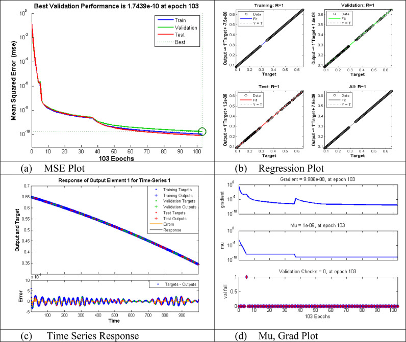
Consider a stochastic Susceptible-Infected-Removed (SIR) model. S(t), I(t) and R (t) denotes the number of susceptible, infected but not lab-confirmed cases (including those in incubation period) and removed population (including recoveries, fatalities and confirmed cases) at time t respectively, and note that N(t)= S (t)+ I (t)+R (t) is a constant. Reproduction number R=, where γ and β are the removing rate and transmission rate. So the stochastic model can be represented in the form of following ODEs [51,52]:-
After solution of above equations by utilizing the computational strength of Neural Network and graphical outcomes can be seen in Fig. 17 .
Fig. 17.
Graphical view of the various plot of Comparative SIR Model.
10. Conclusion
In this research, NAR-RBFs based hybrid neural network is presented to model the set of differential equations representing the SITR model. The error term based on stochastic variation is included to model the COVID-19 abrupt spread. This computational technique based on deep learning has shown extraordinary performance in terms of accuracy and convergence. The outcomes of this study will be useful in forecasting the progression of COVID-19 for different countries. The influence of several key parameters in overspread of COVID-19 pandemic are ideally modeled which can help for planning, monitoring as well as preventing measure the spread of COVID-19 pandemic.
In future one may utilize the computational strength of NAR-RBFs hybrid model for the solution of problems [53], [54], [55], [56], [57].
Declaration of Competing Interest
The authors declare no competing interests.
Acknowledgements
The authors acknowledge the financial support provided by the Center of Excellence in Theoretical and Computational Science (TaCS-CoE), KMUTT. Moreover, this research project is supported by Thailand Science Research and Innovation (TSRI) Basic Research Fund: Fiscal year 2021 under project number 64A306000005.
Appendix
The comparative results for proposed computing paradigm through NAR, RBF, and NAR-RBFs based models for all variables in SITR system representing COVID-19 dynamics are presented in Tables A1, A2 and A3 for mentioned scenarios.
References
- 1.Wang C, Horby P W, Hayden FG, Gao G F. A novel coronavirus outbreak of global health concern. Lancet. 2020;395:470–473. doi: 10.1016/S0140-6736(20)30185-9. [DOI] [PMC free article] [PubMed] [Google Scholar]
- 2.National Health Commission of the People's Republic of China. http://www.nhc.gov.cn/xcs/yqfkdt/202002/553ff43ca29d4fe88f3837d49d6b6ef1.shtml, accessed Feb 14, 2020. [DOI] [PMC free article] [PubMed]
- 3.Health Commission of Hubei Province. http://wjw.hubei.gov.cn/fbjd/dtyw/202002/t202002142027187.shtmll, accessed Feb 13, 2020.
- 4.Worldometers. Worldometers coronavirus, 2020.
- 5.Liu X., Hewings G.J., Qin M., Xiang X., Zheng S., Li X., Wang S. 2020. Modelling the situation of COVID-19 and effects of different containment strategies in China with dynamic differential equations and parameters estimation. Available at SSRN 3551359. [Google Scholar]
- 6.Guan W.J., Ni Z.Y., Hu Y., Liang W.H., Ou C.Q., He J.X., Liu L., Shan H., Lei C.L., Hui D.S.C., Du B. China medical treatment expert group for covid-19. Clinical characteristics of coronavirus disease 2019 in China. N. Engl. J. Med. 2020;382(18):1708–1720. doi: 10.1056/NEJMoa2002032. [DOI] [PMC free article] [PubMed] [Google Scholar]
- 7.Ru-guo F.A.N., Yi-bo W.A.N.G., Ming L.U.O., Ying-qing Z.H.A.N.G., Chao-ping Z.H.U. Vol. 49. 2020. pp. 1–6. (SEIR-based novel pneumonia transmission model and inflection point prediction analysis). 电子科技大学学报. [Google Scholar]
- 8.Roosa K., Lee Y., Luo R., Kirpich A., Rothenberg R., Hyman J.M., Yan P., Chowell G. Real-time forecasts of the COVID-19 epidemic in China from February 5th to February 24th, 2020. Infect. Dis. Model. 2020;5:256–263. doi: 10.1016/j.idm.2020.02.002. [DOI] [PMC free article] [PubMed] [Google Scholar]
- 9.Kucharski A.J., Russell T.W., Diamond C., Liu Y., Edmunds J., Funk S., Eggo R.M., Sun F., Jit M., Munday J.D., Davies N. The lancet infectious diseases. 2020. Early dynamics of transmission and control of COVID-19: a mathematical modelling study. [DOI] [PMC free article] [PubMed] [Google Scholar]
- 10.Yang Z., Zeng Z., Wang K., Wong S.S., Liang W., Zanin M., Liu P., Cao X., Gao Z., Mai Z., Liang J. Modified SEIR and AI prediction of the epidemics trend of COVID-19 in China under public health interventions. J. Thorac. Dis. 2020;12(3):165. doi: 10.21037/jtd.2020.02.64. [DOI] [PMC free article] [PubMed] [Google Scholar]
- 11.Ivorra B., Ferrández M.R., Vela-Pérez M., Ramos A.M. Mathematical modeling of the spread of the coronavirus disease 2019 (COVID-19) taking into account the undetected infections. The case of China. Commun. Nonlinear Sci. Numer. Simul. 2020 doi: 10.1016/j.cnsns.2020.105303. [DOI] [PMC free article] [PubMed] [Google Scholar]
- 12.Bonyah E., Khan M.A., Okosun K.O., Islam S. A theoretical model for Zika virus transmission. PLoS One. 2017;12(10) doi: 10.1371/journal.pone.0185540. [DOI] [PMC free article] [PubMed] [Google Scholar]
- 13.Yavuz M., Bonyah E. New approaches to the fractional dynamics of schistosomiasis disease model. Physica A. 2019;525:373–393. [Google Scholar]
- 14.Diekmann O, Heesterbeek H, Britton T. Princeton Series in Theoretical and Computational Biology. Princeton University Press; 2013. Understanding Infectious Disease Dynamics. [Google Scholar]
- 15.Chen Y., Cheng J., Jiang Y., Liu K. A time delay dynamical model for outbreak of 2019-nCoV and the parameter identification. J. Inverse Ill-Posed Probl. 2020;28(2):243–250. [Google Scholar]
- 16.Cantó B., Coll C., Sánchez E. Estimation of parameters in a structured SIR model. Advances in Difference Equations. 2017;2017(1):33. [Google Scholar]
- 17.Stefan M., Yingcun X, editors. Mathematical Understanding of Infectious Disease Dynamics(Vol. 16) World Scientific; 2008. [Google Scholar]
- 18.LIU C., DING G., GONG J. Mathematical modeling on the prediction and warning of SARS. Chin. Sci. Bull. 2004;49(21):2245–2251. [Google Scholar]
- 19.Chinazzi Matteo, Davis Jessica T., Ajelli Marco, Gioannini Corrado, Litvinova Maria, Merler Stefano, Pastore y Piontti Ana, Rossi Luca, Sun Kaiyuan, C´ ecile Viboud Xinyue, Xiong Hongjie, Yu M.Elizabeth, Halloran Ira M. The effect of travel restrictions on the spread of the 2019 novel coronavirus (2019-ncov) outbreak. medRxiv; 2020. Longini, and Alessandro Vespignani. [DOI] [PMC free article] [PubMed] [Google Scholar]
- 20.Jin Gehui, Yu Jiayu, Han Liyuan, Duan Shiwei. medRxiv; 2020. The impact of traffic isolation in wuhan on the spread of 2019-ncov. [Google Scholar]
- 21.Hellewell Joel, Abbott Sam, Gimma Amy, Bosse Nikos I, Jarvis Christopher I, Russell Timothy W, Munday James D, Kucharski Adam J, John Edmunds W, nCoV working group CMMID, Funk Sebastian, Eggo Rosalind M. medRxiv; 2020. Feasibility of controlling 2019-ncov outbreaks by isolation of cases and contacts. [DOI] [PMC free article] [PubMed] [Google Scholar]
- 22.Quilty Billy, Clifford Sam, Flasche Stefan, Eggo Rosalind M. 2020. Effectiveness of airport screening at detecting travellers infected with 2019-ncov. medRxiv. [DOI] [PMC free article] [PubMed] [Google Scholar]
- 23.Bonyah E., Badu K., Asiedu-Addo S.K. Optimal control application to an Ebola model. Asian Pacific J. Tropic. Biomed. 2016;6(4):283–289. doi: 10.1016/j.apjtb.2016.01.012. [DOI] [PMC free article] [PubMed] [Google Scholar]
- 24.Bonyah E., Atangana A., Khan M.A. Modeling the spread of computer virus via Caputo fractional derivative and the beta-derivative. Asia Pacific J. Comput. Eng. 2017;4(1):1. [Google Scholar]
- 25.Settati A., Lahrouz A., Assadouq A., El Fatini M., El Jarroudi M., Wang K. The impact of nonlinear relapse and reinfection to derive a stochastic threshold for SIRI epidemic model. Chaos Solitons Fractals. 2020;137 [Google Scholar]
- 26.Karimi H., Yousefi F. Application of artificial neural network–genetic algorithm (ANN–GA) to correlation of density in nanofluids. Fluid Phase Equilib. 2012;336:79–83. [Google Scholar]
- 27.Ramírez E., Melin P., Prado-Arechiga G. Hybrid Intelligent Systems in Control, Pattern Recognition and Medicine. Springer; Cham: 2020. Hybrid Model Based on Neural Networks and Fuzzy Logic for 2-Lead Cardiac Arrhythmia Classification; pp. 193–217. [Google Scholar]
- 28.Wang J., Du P., Hao Y., Ma X., Niu T., Yang W. An innovative hybrid model based on outlier detection and correction algorithm and heuristic intelligent optimization algorithm for daily air quality index forecasting. J. Environ. Manage. 2020;255 doi: 10.1016/j.jenvman.2019.109855. [DOI] [PubMed] [Google Scholar]
- 29.Gao W., Raftari M., Rashid A.S.A., Mu'azu M.A., Jusoh W.A.W. A predictive model based on an optimized ANN combined with ICA for predicting the stability of slopes. Engineering with Computers. 2020;36(1):325–344. [Google Scholar]
- 30.Cheema T.N., Raja M.A.Z., Ahmad I., Naz S., Ilyas H., Shoaib M. Intelligent computing with Levenberg–Marquardt artificial neural networks for nonlinear system of COVID-19 epidemic model for future generation disease control. The European Physical Journal Plus. 2020;135(11):1–35. doi: 10.1140/epjp/s13360-020-00910-x. [DOI] [PMC free article] [PubMed] [Google Scholar]
- 31.Wieczorek M., Siłka J., Woźniak M. Neural network powered COVID-19 spread forecasting model. Chaos Solitons Fractals. 2020;140 doi: 10.1016/j.chaos.2020.110203. [DOI] [PMC free article] [PubMed] [Google Scholar]
- 32.Marques G., Agarwal D., de la Torre Díez I. Automated medical diagnosis of COVID-19 through EfficientNet convolutional neural network. Appl. Soft Comput. 2020;96 doi: 10.1016/j.asoc.2020.106691. [DOI] [PMC free article] [PubMed] [Google Scholar]
- 33.Khan F.M., Gupta R. Arima and nar based prediction model for time series analysis of covid-19 cases in india. J. Safe. Sci. Resilience. 2020;1(1):12–18. [Google Scholar]
- 34.Umar M., Sabir Z., Raja M.A.Z., Shoaib M., Gupta M., Sánchez Y.G. A Stochastic Intelligent Computing with Neuro-Evolution Heuristics for Nonlinear SITR System of Novel COVID-19 Dynamics. Symmetry. 2020;12(10):1628. [Google Scholar]
- 35.Jung S.Y., Jo H., Son H., Hwang H.J. Real-World Implications of a Rapidly Responsive COVID-19 Spread Model with Time-Dependent Parameters via Deep Learning: Model Development and Validation. J. Med. Internet Res. 2020;22(9):19907. doi: 10.2196/19907. [DOI] [PMC free article] [PubMed] [Google Scholar]
- 36.Naik PA, Yavuz M, Qureshi S, Zu J, Townley S. Modeling and analysis of COVID-19 epidemics with treatment in fractional derivatives using real data from Pakistan. The European Physical Journal Plus. 2020 Oct. 2020;135(10):1–42. doi: 10.1140/epjp/s13360-020-00819-5. [DOI] [PMC free article] [PubMed] [Google Scholar]
- 37.Wang Y., Xu C., Yao S., Zhao Y. Forecasting the epidemiological trends of COVID-19 prevalence and mortality using the advanced α-Sutte Indicator. Epidemiology & Infection. 2020:148. doi: 10.1017/S095026882000237X. [DOI] [PMC free article] [PubMed] [Google Scholar]
- 38.Zeng Tianyu, Zhang Yunong, Li Zhenyu, Liu Xiao, Qiu Binbin. 2020. Predictions of 2019-ncov transmission ending via comprehensive methods. [Google Scholar]
- 39.Huang Norden E, Qiao Fangli. A data driven time-dependent transmission rate for tracking an epidemic: a case study of 2019-ncov. Science Bulletin. 2020 doi: 10.1016/j.scib.2020.02.005. [DOI] [PMC free article] [PubMed] [Google Scholar]
- 40.Read Jonathan M, Bridgen Jessica RE, Cummings Derek AT, Ho Antonia, Jewell Chris P. Novel coronavirus 2019-ncov: early estimation of epidemiological parameters and epidemic predictions. medRxiv. 2020 doi: 10.1098/rstb.2020.0265. [DOI] [PMC free article] [PubMed] [Google Scholar]
- 41.Tang Biao, Wang Xia, Li Qian, Bragazzi Nicola Luigi, Tang Sanyi, Xiao Yanni, Wu Jianhong. Estimation of the transmission risk of the 2019-ncov and its implication for public health interventions. J. Clin. Med. 2020;9(2) doi: 10.3390/jcm9020462. [DOI] [PMC free article] [PubMed] [Google Scholar]
- 42.Tang Biao, Bragazzi Nicola Luigi, Li Qian, Tang Sanyi, Xiao Yanni, Wu Jianhong. Infectious Disease Modelling; 2020. An updated estimation of the risk of transmission of the novel coronavirus (2019-ncov) [DOI] [PMC free article] [PubMed] [Google Scholar]
- 43.Sanchez Y.G., Sabir Z., Guirao J.L. 2020. Design of a nonlinear SITR fractal model based on the dynamics of a novel coronavirus (COVID-19) [Google Scholar]
- 44.Luo W., Majumder M., Liu D., Poirier C., Mandl K., Lipsitch M., Santillana M. 2020. The role of absolute humidity on transmission rates of the COVID-19 outbreak. [DOI] [PMC free article] [PubMed] [Google Scholar]
- 45.Wang M., Jiang A., Gong L., Luo L., Guo W., Li C., Zheng J., Li C., Yang B., Zeng J., Chen Y. MedRxiv; 2020. Temperature significant change COVID-19 Transmission in 429 cities. [Google Scholar]
- 46.Wang Y., Yang J., Mo Y., Xiao C., An W. Disparity estimation for camera arrays using reliability guided disparity propagation. IEEE Access. 2018;6:21840–21849. [Google Scholar]
- 47.López M., Valero S., Senabre C., Aparicio J., Gabaldon A. Application of SOM neural networks to short-term load forecasting: The Spanish electricity market case study. Electric Power Systems Research. 2012;91:18–27. [Google Scholar]
- 48.Ibrahim M., Jemei S., Wimmer G, Hissel D. Nonlinear autoregressive neural network in an energy management strategy for battery/ultra-capacitor hybrid electrical vehicles. Electric Power Systems Research. 2016;136:262–269. [Google Scholar]
- 49.Alwakeel M., Shaaban Z. Face recognition based on Haar wavelet transform and principal component analysis via Levenberg-Marquardt backpropagation neural network. European J. Sci. Res. 2010;42:25–31. [Google Scholar]
- 50.Marquardt, Donald W. An algorithm for least-squares estimation of nonlinear parameters. J. Soc. Indust. Appl. Math. 1963;11:431–441. [Google Scholar]
- 51.Toda A.A. 2020. Susceptible-infected-recovered (sir) dynamics of covid-19 and economic impact. arXiv preprint arXiv:2003.11221. [Google Scholar]
- 52.You C., Deng Y., Hu W., Sun J., Lin Q., Zhou F., Pang C.H., Zhang Y., Chen Z., Zhou X.H. Estimation of the time-varying reproduction number of COVID-19 outbreak in China. Int. J. Hyg. Environ. Health. 2020 doi: 10.1016/j.ijheh.2020.113555. [DOI] [PMC free article] [PubMed] [Google Scholar]
- 53.Faisal F., Shoaib M., Raja M.A.Z. A new heuristic computational solver for nonlinear singular Thomas–Fermi system using evolutionary optimized cubic splines. The European Physical Journal Plus. 2020;135(1):1–29. [Google Scholar]
- 54.Ahmad I., Ilyas H., Urooj A., Aslam M.S., Shoaib M., Raja M.A.Z. Novel applications of intelligent computing paradigms for the analysis of nonlinear reactive transport model of the fluid in soft tissues and microvessels. Neural Computing and Applications. 2019;31(12):9041–9059. [Google Scholar]
- 55.Waseem W., Sulaiman M., Islam S., Kumam P., Nawaz R., Raja M.A.Z., Farooq M., Shoaib M. A study of changes in temperature profile of porous fin model using cuckoo search algorithm. Alexandria Eng. J. 2020;59(1):11–24. [Google Scholar]
- 56.Sabir Z., Raja M.A.Z., Umar M., Shoaib M. Design of neuro-swarming-based heuristics to solve the third-order nonlinear multi-singular Emden–Fowler equation. The European Physical Journal Plus. 2020;135(6) [Google Scholar]
- 57.Sabir Z., Raja M.A.Z., Umar M., Shoaib M. Neuro-swarm intelligent computing to solve the second-order singular functional differential model. The European Physical Journal Plus. 2020;135(6):474. [Google Scholar]


