Global hunger and climate change adaptation through international trade

Abstract

International trade enables us to exploit regional differences in climate change impacts and is increasingly regarded as a potential adaptation mechanism. Here, we focus on hunger reduction through international trade under alternative trade scenarios for a wide range of climate futures. Under the current level of trade integration, climate change would lead to up to 55 million people who are undernourished in 2050. Without adaptation through trade, the impacts of global climate change would increase to 73 million people who are undernourished (+33%). Reduction in tariffs as well as institutional and infrastructural barriers would decrease the negative impact to 20 million (−64%) people. We assess the adaptation effect of trade and climate-induced specialization patterns. The adaptation effect is strongest for hunger-affected import-dependent regions. However, in hunger-affected export-oriented regions, partial trade integration can lead to increased exports at the expense of domestic food availability. Although trade integration is a key component of adaptation, it needs sensitive implementation to benefit all regions.

Approximately 11% of the world population in 2017, or 821 million people, suffered from hunger¹. Undernourishment has been increasing since 2014 due to conflict, climate variability and extremes, and is most prevalent in sub-Saharan Africa (23.2% of population), the Caribbean (16.5%) and Southern Asia (14.8%)¹. Climate change is projected to raise agricultural prices² and to expose an additional 77 million people to hunger risks by 2050 (ref.³), thereby jeopardizing the UN Sustainable Development Goal to end global hunger⁴. Adaptation policies to safeguard food security range from new crop varieties and climate-smart farming to reallocation of agricultural production^2,5.

International trade can be an important adaptation mechanism^6,7. Trade links countries with a food deficit with countries with a food surplus and raises consumption possibilities through specialization according to comparative advantage. Climate change affects regions and crops differently⁸, possibly shifting regional comparative advantages and altering trade patterns. Studies report that restricting trade exacerbates the impact of climate change on agricultural production, whereas liberalizing trade alleviates it^9–14. However, the current literature is incomplete in its scenario design and does not comprehensively assess whether and—if so, why—the role of trade becomes larger under climate change (see Methods; Supplementary Text). The ‘adaptation illusion hypothesis’ argues that many farm practices are wrongly identified as adaptation because they have equal beneficial impacts with or without climate change^15,16. Here we investigated the case of adaptation through trade, and reveal whether climate change alters the pattern of comparative advantage and increases the impact of trade integration on hunger. With the emerging integration between climate and trade policy agendas¹⁷, a better understanding is needed to guide international policies to reduce hunger.

Prevailing trade barriers may affect the adaptation potential of trade. Border protection is widespread and has an important influence on agrifood trade^18,19. Despite substantial liberalization efforts under the ongoing Doha Round, tariffs remain high for agricultural products²⁰. We investigated the impact of pre-Doha tariff levels as well as further liberalization of agricultural tariffs. Other trade costs associated with infrastructure, logistics and custom procedures are high, particularly in agricultural trade and in developing countries²¹. Reducing such barriers could create larger trade gains than reductions in border protection¹⁸. We compared the adaptation potential of trade liberalization, through the reduction in tariff barriers, and trade facilitation, through the reduction in other trade costs.

We focused on global hunger projections to 2050 and analysed how climate change and trade interact in their impact on hunger. Our economic (Global Biosphere Management Model (GLOBIOM)) and crop (Environment Policy Integrated Model (EPIC)) modelling approach (see Methods) is well established for investigating agricultural climate change impacts^22–25. We advance on the current literature by analysing 60 integrated scenarios that capture variability in trade barriers and in climate projections originating from general circulation models (GCMs), emissions scenarios (Representative Concentration Pathways (RCPs)) and assumptions about CO₂ fertilization. By statistically analysing the scenario sample, we assessed whether, where and how climate change influences the effect of trade on the risk of hunger.

The adaptive effect of international trade on global hunger

Building on a previous study²⁴, we used ten climate change and six trade scenarios, and analysed hunger effects at the global and regional levels. Four RCPs (2.6 W m⁻², 4.5 W m⁻², 6.0 W m⁻² and 8.5 W m⁻²) are projected by HadGEM2-ES. RCP 8.5 is also implemented with four alternative climate models (GFDL-ESM2M, NorESM1-M, IPSL-CM5A-LR and MIROC-ESM-CHEM). RCP 2.6 represents climate stabilization at 2 °C, whereas RCP 8.5 represents a probable temperature range of 2.6–4.8 °C (ref.²⁶). We compared the strongest climate change impacts (RCP 8.5) with the intermediate climate scenarios (RCP 2.6 to RCP 6.0). EPIC projects yields for climatic conditions of each RCP × GCM combination including CO₂ fertilization that are compared to yields without climate change impacts (no climate change scenario). RCP 8.5 × HadGEM2-ES was also run without CO₂ fertilization effects, representing the worst possible outcome. Our approach follows the ISI-MIP (www.isimip.org) Fast Track Protocol, which considers scenarios with CO₂ fertilization as the default, and prioritizes RCP 8.5 × HadGEM2-ES for CO₂ sensitivity analyses. We provide a complete CO₂ sensitivity analysis across RCPs in the Supplementary Text. In the baseline trade scenario, trade barriers were kept constant at 2010 level, but trade patterns vary endogenously across different climate impact scenarios. The fixed imports scenario prevents agricultural imports from exceeding levels from the no climate change scenario. The pre-Doha tariffs scenario represents the trade environment before global trade liberalization launched by the Doha Round. In the facilitation scenario, additional costs from expanding trade volume beyond the current level (for example infrastructure costs) were set close to zero. Under the tariff elimination scenario agricultural tariffs were progressively phased out from −25% in 2020 to −100% in 2050. The facilitation + tariff elimination scenario combines the previous two scenarios. Socioeconomic developments were modelled with the second Shared Socioeconomic Pathway (SSP2)²⁷. The scenarios are discussed further in the Methods.

Through adjustments in trade, supply and demand, the 2050 global population at risk of hunger under climate change and trade scenarios deviates substantially from the SSP2 baseline (the baseline trade + no climate change scenario; Fig. 1). Lower trade costs reduce importer prices, increase traded quantities and/or increase exporter prices, whereas lower climate-induced crop yields increase prices. On the supply side, this influences the optimal land allocation within each pixel in terms of land cover, crop and management system. On the demand side, regions determine the optimal level of consumption and trade of each product in response to new price levels. Within-country distributional impacts of price changes through agricultural income effects were not considered (see Methods). In the baseline trade scenario, price changes across RCP 8.5 scenarios lead to a reduction in global food availability of −0.2% to −3% compared with the baseline. The corresponding hunger effects are large—an additional 7–55 million people are projected to become undernourished (+6% to +45%). Across the RCP 8.5 scenarios, global cropland area changes by −2% to +3% and the share of irrigated area increases from +1% to +7%. Total agricultural trade volume increases by +1% to +7% across RCP 8.5 scenarios through an expansion at the intensive and extensive margin (new flows representing 1–3% of total trade volume; Supplementary Table 1). Hunger impacts under intermediate climate change range from a decrease of 1 million to an increase of 14 million undernourished people. In RCP 2.6, undernourishment is lower than in the no climate change scenario because crop yields in several regions increase or remain unaffected partly due to the CO₂ fertilization effect (Extended Data Fig. 1, Supplementary Fig. 12). When adaptation through trade is constrained in the fixed imports scenario, hunger exacerbates across all of the RCP 8.5 scenarios, up to an additional 73 million undernourished people compared with the baseline (+60%). By preventing endogenous market responses to climate change, the fixed imports scenario results in lower global crop production efficiency (−1% to −2.5%), lower global food availability (−10 to −37 kcal per capita per day) and higher agricultural prices (+2% to +17%) across the RCP 8.5 scenarios compared with the baseline trade scenario (Supplementary Table 2). The pre-Doha tariffs scenario leads to up to 81 million additional undernourished people compared with the baseline scenario (+67%), highlighting the importance of trade integration that has already been achieved through the Doha Round in alleviating the potential long-term impacts of climate change on hunger.

Fig. 1 |. Global population at risk of hunger in 2050 across climate change and trade scenarios.

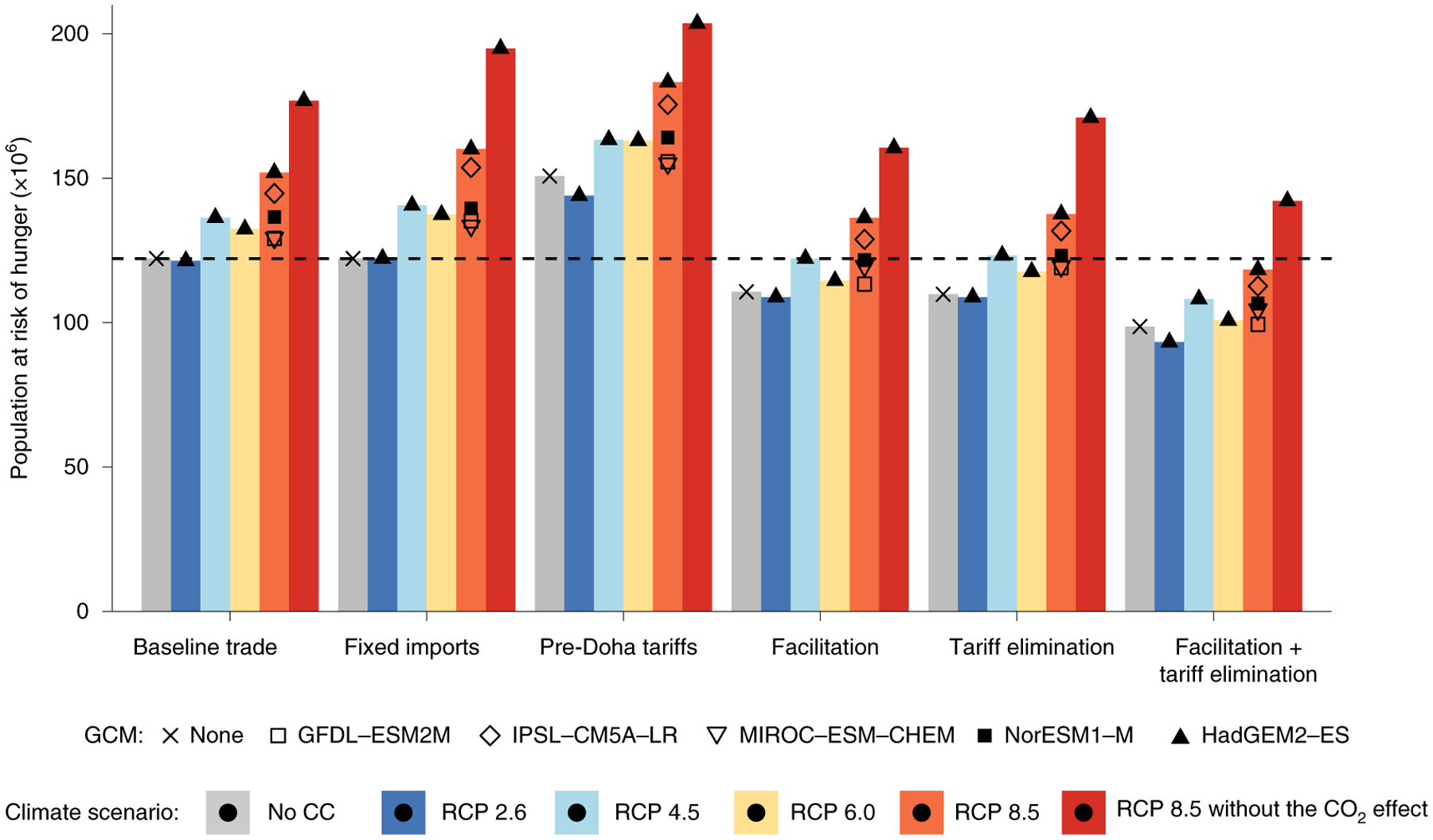
Climate change scenarios include the effect of CO₂ fertilization on crop yields. RCP 8.5 is implemented with and without the CO₂ effect. The black dotted horizontal line indicates the population at risk of hunger in the SSP2 baseline (122 million).

The facilitation and tariff elimination scenarios reduce the global risk of hunger from climate change to a comparable extent, and the facilitation + tariff elimination scenario can even compensate for the impact of all but the most extreme climate change scenario. Trade liberalization and facilitation reduce hunger by enhancing climate-induced trade adjustments—across RCP 8.5 scenarios, total agricultural trade increases by 166% to 262% under the facilitation + tariff elimination scenario—by reducing agricultural prices, and by increasing food availability and crop production efficiency (Supplementary Tables 1 and 2). The hunger effect under extreme climate change (RCP 8.5 without the CO₂ effect) is reduced by 31% under the facilitation scenario, 11% under the tariff elimination scenario and 64% under the facilitation + tariff elimination scenario. These effects are consistent with other studies that reported 44% lower hunger effects under market integration¹³ and 46% lower price effects under trade liberalization¹⁰ (Supplementary Fig. 5).

Regional perspective on climate change, hunger and trade

The hunger outcomes of the climate and trade scenarios differ substantially among the hunger-affected regions (Fig. 2). Climate change has little impact on regions facing positive or small negative crop yield impacts (Russia and West Asia (CSI), and the Middle-East and North-Africa (MNA)) or maintaining a high crop yield (Latin American countries (LAC); Extended Data Fig. 1 (for average crop yield), Supplementary Figs. 1–4 (for the four main crops)). Regions with negative impacts on medium crop yields face larger hunger impacts (East Asia (EAS) and Southeast Asia (SEA)). South Asia (SAS) and sub-Saharan Africa (SSA) face the most severe hunger impacts from climate change. They experience negative impacts on already low yields, also when including the impact of supply-side adaptation on yields (Extended Data Fig. 2). Across the RCP 8.5 scenarios, projections for the baseline trade scenario range from an increase of 13–181% and 2–51% in the population at risk of hunger for SAS and SSA, respectively. The effect of the trade scenarios on regional undernourishment is largest among baseline net-importing regions (SSA, MNA, EAS and SAS) and regions in which climate change reduces net exports (SEA; Extended Data Figs. 3 and 4). The fixed imports scenario enlarges hunger impacts in the extreme climate change scenario in SSA, SAS and SEA by raising agricultural prices (Extended Data Figs. 5 and 6), increasing net exports in SEA, and reducing net imports in SSA and SAS. Adverse effects from trade restriction, such as the export bans observed during the 2007–2008 world food crisis^28,29 and those feared as a result of the global COVID-19 pandemic^30,31, may pose severe hunger risks under climate change. Under the pre-Doha tariffs scenario undernourishment in SSA, SAS and EAS is substantially higher compared with the baseline trade scenario. Tariff liberalization between 2001 and 2010 reduced average import tariffs in SSA, SAS and EAS by around 30% (Supplementary Table 6). The lower tariffs reduce the overall level of trade costs by 2050 (Supplementary Table 7) and enable larger agricultural net imports in SSA, SAS and EAS across all climate scenarios (Extended Data Fig. 3). In the MNA region, the average import tariff reduced marginally and in SEA it was already low (Supplementary Table 6). The facilication + tariff elimination scenario reduces hunger in the SSA, MNA and EAS regions across all climate scenarios by decreasing average trade costs (Supplementary Table 7), thereby reducing agricultural prices and raising agricultural imports (Extended Data Figs. 3 and 5). In some cases, trade integration increases rather than decreases the level of undernourishment in a region under climate change. The largest adverse effects occur under the tariff elimination scenario in the SEA and SAS regions (Extended Data Fig. 7). Whereas the facilitation scenario reduces hunger in the extreme climate change scenario by 16% and 8%, the tariff elimination scenario increases hunger impacts by 4% and 16% in SEA and SAS, respectively. Both trade scenarios reduce average trade costs (Supplementary Table 7), but the tariff elimination scenario increases rice exports from SAS and SEA, thereby reducing domestic calorie availability. The facilication + tariff elimination scenario compensates for calorie loss from rice exports through increased imports of other agricultural goods and decreases the hunger effect of extreme climate change by 26% and 11% in SEA and SAS, respectively. Our sensitivity analysis shows that the effects of trade on climate-induced hunger are robust to CO₂ fertilization assumptions (Supplementary Figs. 13 and 14).

Fig. 2 |. Population at risk of hunger in 2050 across climate change and trade scenarios in each region.

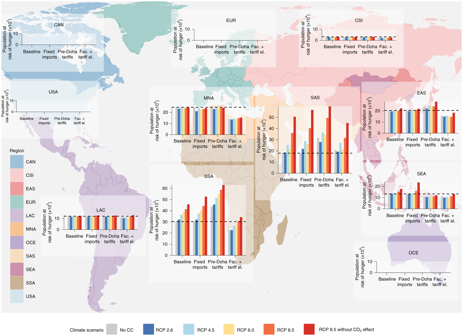
The results from the GCM HadGEM2–ES are shown; the full scenario set is provided in Extended Data Fig. 7. The following regions are included: USA, Russia and West Asia (CSI), East Asia (EAS), Southeast Asia (SEA), South Asia (SAS), Middle East and North Africa (MNA), sub-Saharan Africa (SSA), Latin American Countries (LAC), Oceania (OCE), Canada (CAN) and Europe (EUR). The black dotted horizontal lines indicate the population at risk of hunger in the SSP2 baseline. Fac. + tariff el., facilitation + tariff elimination.

A larger role for trade under climate change

To reveal whether the effect of trade increases under climate change and, therefore, has a real adaptation role, we analysed hunger outcomes from GLOBIOM on crop yield shifts projected by EPIC and average trade costs in regional-level regression models (Table 1). We interpret these results for a 5.4% reduction in crop yields and a 23% reduction in average trade costs, which correspond to the average impacts of climate change and the trade integration scenarios, respectively. Regression results revealed that a 5.4% reduction in crop yields within a region leads to an average food availability reduction of 11 kcal per capita per day (95% confidence interval (CI), 15–8 kcal per capita per day) and an additional 0.52 million people at risk of hunger (CI = 0.25–0.79 million). For a 23% decrease in trade costs, we project an increase in average food availability within a region of 13 kcal per capita per day (CI = 9–16 kcal per capita per day) and a decrease in undernourished people of 1.22 million (CI = 1.52–0.93 million). When excluding regions that experience negative impacts in some trade scenarios (SAS and SEA), we found a significant negative interaction effect between trade costs and crop yields (P = 0.014). For example, under extreme climate change (that is, a 20% crop yield reduction), the positive effect of a 23% reduction in trade costs is 1.97 million fewer people undernourished, consisting of a direct (−1.50 million) and a climate-induced trade effect (−0.47 million). These results confirm the existence of positive trade effects on food availability and hunger alleviation^13,32 and reveal an additional climate-induced effect of lowering trade costs.

Table 1 |.

Results from OLS estimation of the impact of crop yields, trade costs and their interaction on regional hunger and food availability

	Population at risk of hunger (million)		Food availability (kcal per capita per day)
Sample	(1) All regions	(2) Without SAS and sea	(1) All regions	(2) Without SAS and SEA
Crop yield (percentage change)	−9.70***	−1.80	213.00***	173.00***
	(2.60)	(1.40)	(29.00)	(31.00)
Trade cost (log[US$/106kcal])	4.70***	5.80***	−49.00***	−80.00***
	(0.58)	(0.73)	(7.40)	(9.40)
Crop yieldxtrade cost	3.30	−8.90**	14.00	191.00***
	(6.20)	(3.60)	(60.00)	(74.00)

^*P < 0.1;

^**P < 0.05;

^***P < 0.01. Regional fixed effects are included. The values in brackets show the heteroskedastic robust s.e.; n = 550 (1) and n = 450 (2). Adjusted R² = 0.890 (1) and adjusted R² = 0.930 (2) for the hunger regressions; and adjusted R² = 0.950 (1) and adjusted R² = 0.920 (2) for the food availability regressions. Observations are GLOBIOM output for the 11 world regions under 5 different trade scenarios (baseline, pre-Doha tariffs, facilitation, tariff elimination and facilitation + tariff elimination) and ten climate change scenarios in 2050. The regression models are described in the Methods.

We ran the regressions presented in Table 1 with regional interaction effects (Supplementary Table 3). In most of the regions, climate-induced decreases in crop yields reduce food availability and increase hunger while reduced trade costs have opposite effects. The food availability impacts of crop-yield changes are largest for SAS, SSA and SEA, whereas the effect of trade costs is largest for regions maintaining net imports under climate change (SSA, MNA and EAS). The corresponding impact on hunger is largest in low-income regions (SSA and SAS), followed by middle-income regions (EAS, MNA, and SEA). The interaction effect, which reveals whether climate change alters the relationship between trade costs and hunger, is most pronounced in SSA, followed by EAS. Figure 3 plots the predicted hunger-yield relationship in EAS and SSA for different levels of trade cost, showing that hunger is less sensitive to climate-induced yield changes under reduced trade costs.

Fig. 3 |. Fitted linear response of population at risk of hunger to climate-induced crop yield change in EAS and SSA for different values of trade costs.

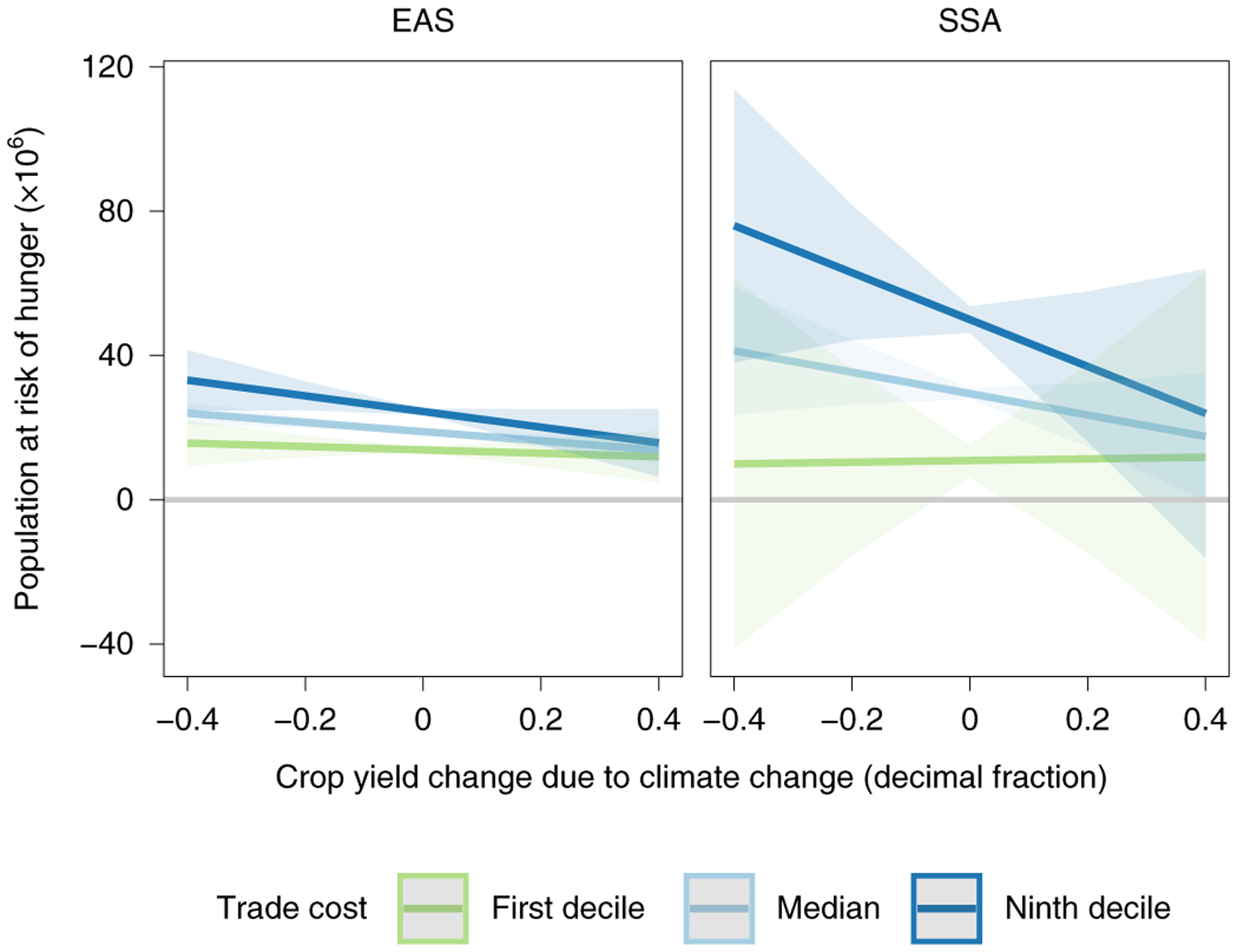
The shaded areas indicate the 95% prediction intervals. Prediction on the basis of an ordinary least squares (OLS) estimation of the regional level linear regression of the impact of crop yield change, trade costs and their interaction on population at risk of hunger. The regression results are shown in Supplementary Table 3 and the regression model is described in the Methods. The fitted response for all of the regions is shown in Extended Data Fig. 8.

Inter-regional specialization

We assessed the extent that climate change shifts the pattern of comparative advantage of four important crops (corn, wheat, soya and rice; Fig. 4). Consistent with Ricardo’s theory of comparative advantage, a region is regarded as having a comparative advantage when it specializes in a certain crop, such that its share of world production increases when trade costs decrease (see Methods; Supplementary Text). Under no climate change, trade integration increases the global production share of the United States (USA) in corn; LAC in soya; CSI, Europe (EUR) and LAC in wheat; and SAS and EAS in rice (Fig. 4a). Trade integration has similar impacts on specialization under climate change (Fig. 4b). Figure 4c compares the specialization of regions in response to trade-cost reduction; negative values indicate decreases and positive values indicate increases in comparative advantage under climate change compared with no climate change. For example, MNA still decreases its share of global wheat production in response to trade integration under climate change, but to a lesser extent than under no climate change. The small and mainly insignificant values indicate that the pattern of comparative advantage of the four crops remains similar under climate change. Although climate change affects crop yields and cost competitiveness of regions, it does not substantially alter the relative position between regions (Supplementary Figs. 8–10). This finding is corroborated by alternative indicators of comparative advantage, including crop shares in a region’s total production, export shares in a region’s crop production and the revealed comparative advantage (RCA) index (Supplementary Figs. 6, 7 and 11).

Fig. 4 |. Inter-regional specialization in corn, rice, soya and wheat in response to trade-cost reduction in 2050.

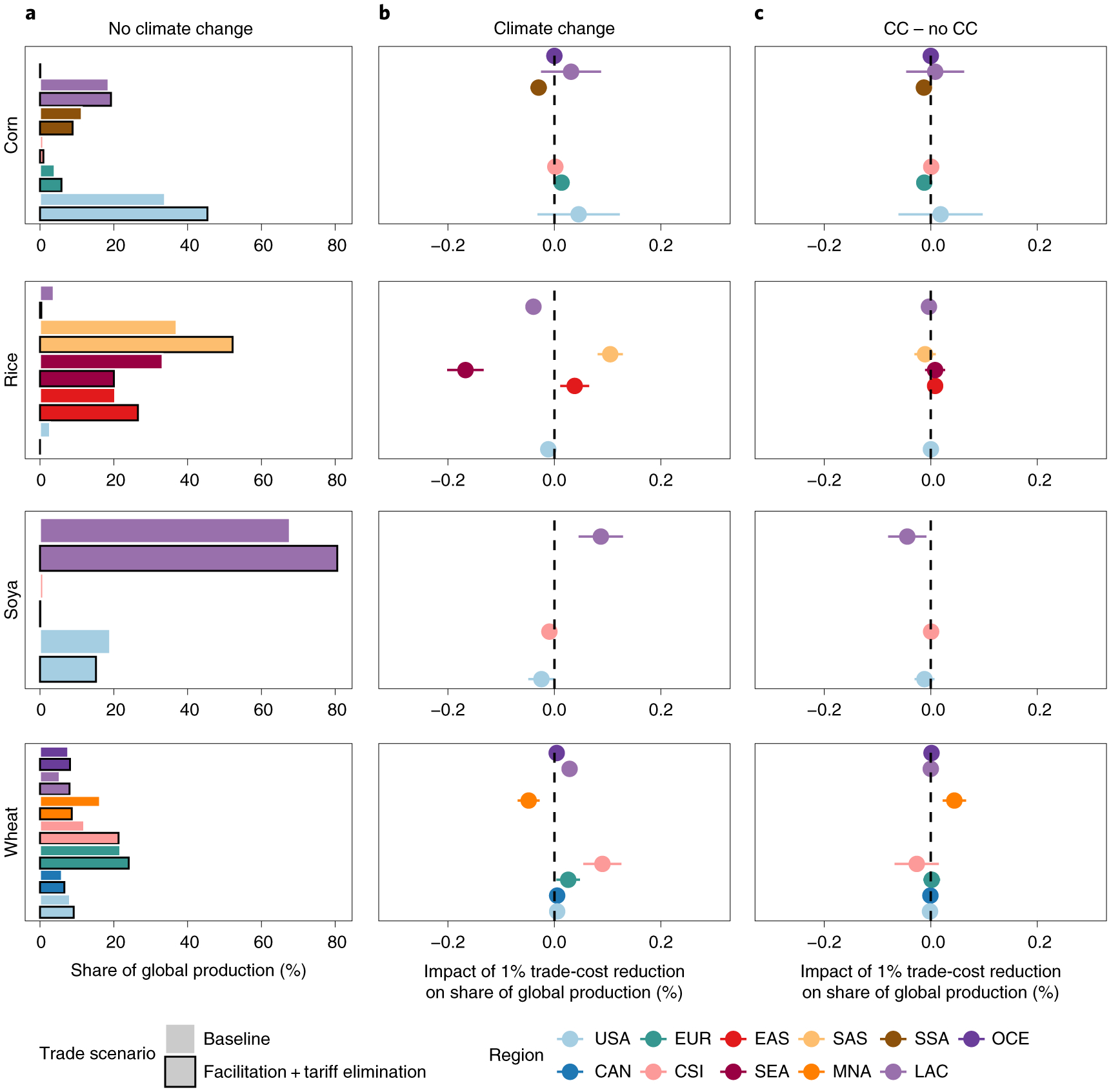
a, The share of global production under no climate change in the baseline trade and facilitation + tariff elimination scenarios. b,c, The impact of 1% trade-cost reduction on the share of global production where the dependent variable is either the outcome under climate change (b) or the difference in outcome between climate change (CC) and no climate change (c). Each point shows the estimated impact of a 1% trade-cost reduction for each region on share of world production (%), with lines denoting the corresponding 95% confidence interval (heteroskedastic robust s.e.). The regression models are described in the Methods.

Adaptation to climate change occurs through changes in existing and new inter-regional trade flows (Supplementary Tables 8–11). Across the RCP 8.5 scenarios, the largest export growth originates from major baseline producing regions (corn from USA and LAC, soya from LAC and USA, rice from SAS and SEA, and wheat from EUR and Canada (CAN); Supplementary Fig. 9). The largest new trade flows are new corn exports from USA to EAS, CAN, LAC and SEA, from EUR to MNA and from LAC to EAS; new soya exports from LAC to SAS and from USA to CAN and MNA; and new wheat exports from CSI to EUR, and from MNA to SSA. Climate change does not induce substantial new rice trade flows. There is uncertainty across RCP 8.5 scenarios in bilateral trade patterns, but several exports to hunger-affected regions increase consistently (such as wheat from EUR to SSA, soya from LAC to SAS, or corn from LAC to MNA). However, hunger-affected regions are not only engaging in trade at the importer side, but also increase certain exports (wheat in MNA, corn in SSA, and rice in EAS and SAS; Extended Data Fig. 10).

Discussion

International trade contributes globally to climate change adaptation. The impact of the worst climate change scenarios on global risk of hunger increases by 33–47% under restricted trade scenarios, and decreases by 11–64% under open trade scenarios. The gain from reducing trade costs is largest for regions that remain import dependent under climate change. Climate change increases the role of trade in reducing the risk of hunger for some regions, although it does not substantially alter the pattern of comparative advantage of main staple crops. It is the ability to link food surplus with deficit regions that underpins trade’s adaptation effect. These conclusions are robust across RCPs, and independent from the assumption on CO₂ fertilization effects. Finally, we found that the number of undernourished people increases with climate change, irrespective of trade scenarios. Thus, climate change mitigation remains crucial for eradicating hunger.

Our study is comprehensive in its scenario design and rigorous in its analysis of the processes driving adaptation through trade. Nevertheless, it is important to emphasize that this study focuses on the global scale in the long term. Trade policies and climate change have important within-country distributional consequences through income and food-access effects^33–35, which are theoretically ambiguous and which our modelling approach does not consider. Across households with different food access channels, from urban net-consumers to rural subsistence farmers, impacts can differ even in their direction³⁴. Also, current global studies, including ours, focus on crop- and grass-yield impacts, and other direct and indirect climate change effects are not represented to date—for example, heat stress on animals, pest and disease incidence, sea level rise or reduced pollination. Finally, we take a long-term equilibrium perspective ignoring the negative effects of extreme weather events. All of these aspects require substantial new research.

Despite the limitations described above, our study brings novel policy implications. We found that liberalization that has already been achieved under the Doha Round substantially reduces climate-induced hunger impacts. A careful approach to trade integration covering different types of trade barriers can further limit hunger risks. The full removal of agricultural tariffs leads to increases in food availability in SSA, MNA and EAS, but may increase exports and lower regional food availability in SEA and SAS. Further trade facilitation can reduce undernourishment in all hunger-affected regions. However, the effective realization of trade facilitation requires considerable investments in transport infrastructure and technology. Especially in low-income regions, such as SSA, infrastructure is weak³⁶. An estimated US$130–170 billion a year is needed to bridge the infrastructure gap in SSA by 2025 (ref.³⁷). Infrastructure finance averaged US$75 billion in recent years, with the largest contribution from budget-constrained national governments³⁷. Alternative financing through institutional and private investments, called for by the African Development Bank Group and the World Bank Group^36,37, could be not only crucial for economic growth, but also for climate change adaptation. In essence, our results demonstrate that trade instruments can mitigate an important part of the adverse hunger effects of long-term climate change. Our results thereby confirm the importance of holistic approaches to international trade negotiations, and could prove also relevant in the face of trade-policy reactions in more acute crisis situations, such as the global COVID-19 pandemic.

Methods

Modelling framework.

We used the GLOBIOM, a recursive dynamic, spatially explicit, economic partial equilibrium model of the agriculture, forestry and bioenergy sector with bilateral trade flows and costs that can model new trade patterns³⁸. The model computes a market equilibrium in 10-year time steps from 2000 to 2050 by maximizing welfare (the sum of consumer and producer surplus) subject to technological, resource and political constraints. In each time step, market prices adjust endogenously to equalize supply and demand for each product and region. On the demand side, a representative consumer for each of 30 economic regions optimizes consumption and trade in response to product prices and income. Food demand depends endogenously on product prices through an isoelastic demand function and exogenously on GDP and population projections³⁹. We mainly present model results aggregated to 11 regions (Supplementary Table 4): USA, CAN, EUR, OCE, SEA, SAS, SSA, MNA, EAS, CSI and LAC. GLOBIOM is a bottom-up model that builds on a high spatial grid-level resolution on the supply side. Land is disaggregated into simulation units—clusters of 5 arcmin pixels that are created based on altitude, slope and soil class, 30 arcmin pixels, and country boundaries. GLOBIOM’s crop production sector includes 18 major crops (barley, beans, cassava, chickpeas, corn, cotton, groundnut, millet, palm oil, potato, rapeseed, rice, soybean, sorghum, sugarcane, sunflower, sweet potato and wheat) under 4 management systems (irrigated, high input; rainfed, high input; rainfed, low input; and subsistence). The allocation of acreage by the crop and management system is determined by potential yields, production costs and expansion constraints²³. Crop production parameters are based on the detailed biophysical crop model EPIC. Additional biophysical models were used to represent the livestock (RUMINANT⁴⁰) and forestry (G4M⁴¹) sectors. Further information on model structure and parameters was described previously^42,43.

As a partial equilibrium model, GLOBIOM focuses only on specific sectors of the economy and does not represent feedbacks on consumer income and GDP from trade and climate change. However, the partial equilibrium model allows for more detail in the represented sectors, and a more accurate assessment of biophysical impacts. This is due to the high spatial and commodity resolution as well as the physical rather than monetary representation of variables compared with the general equilibrium models that explicitly cover income feedbacks. Crop yields adjust endogenously through the management system or location of production, and exogenously according to long-term technological development and climate change impacts²³. The output from EPIC was used to compute, for each time step, yield shifters for each climate change scenario and each crop and management system at a disaggregated spatial scale (simulation unit). EPIC simulates scenario-specific yields on the basis of inputs from climate models (daily climatic conditions including solar radiation, minimum and maximum temperature, precipitation, wind speed, relative humidity and CO₂ concentration). Climate change impacts on livestock production are modelled through crop and grassland yield impacts on feed availability. EPIC crop and grassland yield impacts, as well as their implementation in GLOBIOM, are further explained in Leclère et al.²³ and Baker et al.²⁴.

International trade.

International trade is represented in GLOBIOM through the Enke-Samuelson-Takayama-Judge spatial equilibrium assuming homogenous goods^38,44. Bilateral trade flows between the 30 economic regions were determined by the initial trade pattern, relative production costs of regions and the minimization of trading costs³⁸. The initial trade pattern was informed by the BACI database from CEPII averaging across 1998–2002 (ref.⁴⁵). Trade costs are composed of tariffs from the MAcMap-HS6 database⁴⁶, transport costs⁴⁷ and a nonlinear trade expansion cost. The MAcMap-HS6 2001 release from CEPII-ITC provides ad valorem and specific tariffs, and shadow tariff rates of tariff rate quotas for the model calibration in the base year 2000 (ref.⁴⁸). To incorporate trade liberalization developments under the Doha Round, the tariff data is updated in the 2010 time step with the 2010 release of MAcMap-HS6 (ref.⁴⁹; Supplementary Table 6). We used the estimation by Hummels⁴⁷ to compile input data on bilateral transport costs on the basis of the distance between trade pairs and the weight-value ratio of agricultural products. Transport costs were set to US$30 per ton minimum, on the basis of the fifth percentile of the OECD Maritime Transport Cost database (2003–2007), and were kept constant at base year level over the simulation period as the drivers of transport costs (for example, fuel prices and containerization⁵⁰) are not represented in the partial equilibrium model. In the scenario simulations, the nonlinear expansion cost raises per-unit trade costs when the traded quantity increases over time to model persistency in trade flows. A constant elasticity function was used for trade flows observed in the base year, and a quadratic function was used for new trade flows. The nonlinear element reflects the cost of trade expansion in terms of infrastructure and capacity constraints in the transport sector and was reset after each 10-year time step. Compared to other global economic models, GLOBIOM’s trade representation is positioned between the rigid Armington approach of general equilibrium models and the flexible world pool market approach of many partial equilibrium models.

Risk of hunger.

We measured the population at risk of hunger, or the number of people whose food availability falls below the mean minimum dietary energy requirement, on the basis of previous studies^51–53. The following four parameters were used: the mean minimum dietary energy requirement, the coefficient of variation of the distribution of food within a country, the mean food availability in the country (kcal per capita per day) and total population. Minimum dietary energy requirements are exogenously calculated on the basis of demographic composition (age, sex) of future population projections. Future changes in the inequality of food distribution within a country are exogenous and follow projected national income growth. This is based on an estimated relationship between income and the coefficient of variation of food distribution with observed historical national-level data. Poor infrastructure, remoteness and a high prevalence of subsistence farming limit local markets in distributing food equally across households⁷. Income is lowest in SAS and SSA, regions in which the share of land under subsistence farming is the largest (27% in SAS and 43% in SSA)⁵⁴. Food availability in kcal per capita per day is endogenously determined by GLOBIOM at the regional level. One limitation of the approach is that it does not include within-country distributional consequences of trade integration and/ or climate change through income effects. Trade policies and climate change alter food prices, which affects individual incomes, purchasing power and food access depending on households being net consumers or net producers of food³³. At the aggregate regional level, the bias from not considering these distributional effects may be upward or downward, depending on the share of net-consuming versus net-producing households; degree of subsistence farming versus agricultural wage work; and share of rural versus urban population in each country.

Climate change adaptation.

Climate change adaptation is defined by the IPCC as “the process of adjustment to actual or expected climate and its effects”²⁶. Adaptation of the agricultural sector to climate-induced changes in crop yields may include adjustments in consumption, production and international trade². Demand-side adaptation is captured in GLOBIOM by changes in regional consumption levels in response to market prices. Supply-side adaptation includes the reallocation of land for each crop by a grid-cell and management system, and the expansion of cropland to other land covers²³. Whereas Leclère et al.²³ assess supply-side adaptation, here we focused on international market responses, in which our analysis approach is inspired by the ‘adaptation illusion hypothesis’ postulated by Lobell¹⁵ and confirmed by Moore et al.⁵⁵. They argue that farm-level practices identified as adaptation measures by many crop modelling studies cannot be referred to as climate adaptation as they have the same yield impact in current climate as under climate change. In a similar manner, we intended to investigate whether, where and, if so, why trade integration has a larger positive impact on the risk of hunger under climate change. We defined the adaptation effect of trade as the sum of the effect of reducing trade costs on hunger under current climate (direct trade effect), and any additional positive or negative impact of trade integration under climate change (climate-induced trade effect). The adaptation effect of trade can be understood through Ricardo’s theory of comparative advantage (Supplementary Text)^11,12. Reducing trade costs promotes trade according to comparative advantage⁵⁶ and facilitates the role of trade as a transmission belt in linking food-deficit and food-surplus regions⁵⁷. Climate change impacts differ across crops and regions⁸. Depending on the spatial distribution of these impacts, the current pattern of comparative advantage may be intensified, maintained or substantially altered. This may lead to increased food deficits in certain regions. Trade is argued to have a larger role under climate change as it facilitates adjustment to changes in comparative advantage^11,12 and enables food surplus to be linked with food deficit regions^6,7,57.

Scenario design.

Our choice of climate change scenarios was determined by the ISI-MIP Fast Track Protocol used by crop modellers to calculate crop and grass yield impacts^8,58. We used all four RCPs that reflect increasing levels of radiative forcing by 2100 (the 2.6 W m⁻², 4.5 W m⁻², 6 W m⁻² and 8.5 W m⁻² scenarios)⁵⁹ as projected by the HadGEM2-ES GCM^60,61. RCP 8.5 was implemented with four additional GCMs to reflect uncertainty in climate models: GFDL-ESM2M⁶², IPSL CM5A-LR⁶³, MIROC-ESM-CHEM⁶⁴ and NorESM1-M⁶⁵. RCP 2.6 represents climate stabilization at 2 °C and RCP 8.5 a temperature range of 2.6–4.8 °C (ref.²⁶). Yield impacts are based on simulations from the crop model EPIC^23,24. Each RCP × GCM combination was modelled including CO₂ fertilization effects. RCP 8.5 × HadGEM2-ES was additionally simulated without the CO₂ effect, which reflects the most severe climate change scenario. These scenarios represent the tier 1 set of ISI-MIP scenarios and climate change impacts are simulated individually for all 18 GLOBIOM crops, except for oil palm, and for grasslands. Scenarios without CO₂ fertilization for RCPs other than RCP 8.5 were considered to be of secondary importance in the ISI-MIP Fast Track—and in the latest simulation protocol for ISI-MIP 3b—and were therefore available only for the four main crops (corn, rice, soya and wheat). We carry out a comprehensive sensitivity analysis with respect to the CO₂ fertilization effect for all RCPs, however, as this requires extrapolating climate change impacts from the four crops to the other crops, and thus would introduce inconsistency with the Tier 1 scenarios, the analysis is presented separately in Supplementary Text. In the no climate change scenario, exogenous yield change originates only from long-term technological development assumptions.

We implemented six trade scenarios to analyse the role of trade in climate change adaptation. The first scenario—fixed imports—limits imports to the level observed in the no climate change scenario or less. This represents restricting trade flow adjustments in response to climate change, or limiting trade as an adaptation mechanism. The second scenario, pre-Doha tariffs, excludes the tariff update in 2010, representing the trade environment before global trade liberalization launched by the Doha Round (a comparison of average tariff rates is provided in Supplementary Table 6). We also implemented three trade integration scenarios to assess promotion of the trade adaptation mechanism. In the first scenario, the facilitation scenario, the nonlinear part of trade costs is set close to zero from 2020 onwards on the basis of Baker et al.²⁴. This reflects the impact of reducing transaction costs, infrastructure costs and other institutional barriers limiting the expansion of trade. Trade facilitation is defined by the WTO as the “simplification of trade procedures”⁶⁶. In economic literature it refers to the reduction in trade transaction costs that are determined by the efficiency of customs procedures, infrastructure services and domestic regulations^18,66. Other trade costs that are relevant in agricultural trade, which were not included in this study, are non-tariff measures (NTMs). UNCTAD defines NTMs as “all policy-related trade costs incurred from production to final consumer, with the exclusion of tariffs”⁶⁷. Typical examples of NTMs are technical measures, such as sanitary and phytosanitary measures (SPS), and price and quantity control measures, such as quotas and subsidies. Some studies include also the above-mentioned transaction costs in the category of NTMs^68,69, whereas others make the explicit distinction^18,70. The per-unit transport costs were kept constant at the base year level. In the second scenario, tariff elimination, all agricultural tariffs were progressively phased out between 2020 and 2050, that is −25% in 2020, −50% in 2030, −75% in 2040 and −100% in 2050. This scenario leads to a 70% growth in total agricultural trade (Supplementary Table 1), comparable in magnitude to the agricultural import (+36%) and export (+60%) growth under tariff liberalization reported by Anderson and Martin⁷¹. The final scenario, facilitation + tariff elimination, is a combination of the previous two scenarios and presents the most extensive open trade scenario. In the baseline trade scenario, trade barriers are kept constant at 2010 levels, but trade patterns vary endogenously across the different climate impact scenarios. Supplementary Table 7 provides a comparison of average trade costs across the different scenarios.

Socioeconomic developments were modelled according to the SSP2, which reflects a middle-of-the-road scenario in which the population reaches 9.2 billion by 2050 and income grows according to historical trends in each region²⁷. The technological development assumed by SSP2 leads to an increase in global average crop yields of 66% between 2000 and 2050 (Supplementary Table 12). The SSP scenarios are widely discussed and are often used as a basis for harmonizing key macroeconomic assumptions for integrated assessment modelling of different climate futures⁷². SSP2 projects a decrease in the global population at risk of hunger from 867 million in 2000 to 122 million by 2050. This because of an increase in food consumption—global food availability increases from 2,700 to 3,007 kcal per capita per day—and an improved food distribution within regions, which are both related to the assumed income growth under SSP2 (ref.⁵³). Income projections lead to changes in food preferences. Under SSP2, the share of livestock products in diets increases globally from 16% in 2000 to 17.3% in 2050, with the largest increases in Asian regions⁷³. Such changes affect the baseline trade pattern—for example, increased production and consumption of livestock products in SAS, EAS and SEA imply an increase in imports of feed crops such as corn and soya by 2050.

Hunger statistical analysis.

We analysed the results of the scenario runs using a regional-level linear regression model to infer the underlying relationship between trade costs, crop-yield changes and hunger as predicted by GLOBIOM. The following models were estimated using OLS (Table 1):

$$\begin{gathered} {\text{ Population at risk of hunger }}_{\mathit{\text{itr}}}= \\ {\beta }_1^{(1)}\text{Crop}{\text{yield}}_{\mathit{\text{ir}}}+{\beta }_2^{(1)}\text{Trade}{\text{costs}}_{\mathit{\text{itr}}} \\ +{\beta }_3^{(1)}{\text{ Crop yield }}_{\mathit{\text{ir}}}\times {\text{ Trade costs }}_{\mathit{\text{itr}}}+\sum _i{\beta }_{4i}^{(1)}{\text{ Region }}_i+{\epsilon }_{\mathit{\text{itr}}}^{(1)} \end{gathered}$$

$$\begin{gathered} {\text{ Food availability }}_{\mathit{\text{itr}}}= \\ {\beta }_1^{(2)}{\text{ Crop yield }}_{\mathit{\text{ir}}}+{\beta }_2^{(2)}{\text{ Trade costs }}_{\mathit{\text{itr}}} \\ +{\beta }_3^{(2)}{\text{ Crop yield }}_{\mathit{\text{ir}}}\times {\text{ Trade costs }}_{\mathit{\text{itr}}}+\sum _i{\beta }_{4i}^{(2)}{\text{ Region }}_i+{\epsilon }_{\mathit{\text{itr}}}^{(2)} \end{gathered}$$

We estimated the models also with regional interaction terms (Fig. 3, Supplementary Table 3):

$$\begin{gathered} {\text{ Population at risk of hunger }}_{\mathit{\text{itr}}}= \\ \sum _i\left({\beta }_{1i}^{(3)}{\text{ Crop yield }}_{\mathit{\text{ir}}}\times {\text{ Region }}_i+{\beta }_{2i}^{(3)}{\text{ Trade costs }}_{\mathit{\text{itr}}}\times \right.{\text{ Region }}_i \\ +{\beta }_{3i}^{(3)}{\text{ Crop yield }}_{\mathit{\text{ir}}}\times {\text{ Trade costs }}_{\mathit{\text{itr}}}\times {\text{ Region }}_i+{\beta }_{4i}^{(3)}\text{ Region }\left.{}_i\right)+{\epsilon }_{\mathit{\text{itr}}}^{(3)} \end{gathered}$$

$$\begin{gathered} {\text{ Food availability }}_{\mathit{\text{itr}}}= \\ \sum _i\left({\beta }_{1i}^{(4)}{\text{ Crop yield }}_{\mathit{\text{ir}}}\times {\text{ Region }}_i+{\beta }_{2i}^{(4)}{\text{ Trade costs }}_{\mathit{\text{itr}}}\times \right.{\text{ Region }}_i \\ +{\beta }_{3i}^{(4)}{\text{ Crop yield }}_{\mathit{\text{ir}}}\times {\text{ Trade costs }}_{\mathit{\text{itr}}}\times {\text{ Region }}_i+{\beta }_{4i}^{(4)}\text{ Region }\left.{}_i\right)+{\epsilon }_{\mathit{\text{itr}}}^{(4)} \end{gathered}$$

where Population at risk of hunger_itr gives the number of people at risk of hunger (million) and Food availability_itr gives the food availability (kcal per capita per day) in 2050 in each region i, trade scenario t and climate change scenario r. Crop yield_ir gives the change in average crop yield (kcal ha−1) compared with the average crop yield in the no climate change scenario in 2050. Trade cost_itr gives the log-transformed weighted average trade costs (US$ per 10⁶ kcal) on all trade flows in 2050. To obtain a measure that reflects the implication of trade scenarios on overall trading costs, we calculated the trade-weighted average of trade costs over all agricultural imports, exports and intraregional trade flows for each region i, trade scenario t and climate change scenario r: ${\text{ Average trade cost }}_{\mathit{\text{itr}}}=\sum _k\frac{x_{\mathit{\text{iktr}}}}{{\text{Total}}_{x_{\mathit{\text{itr}}}}}\times {\text{ Trade cost }}_{\mathit{\text{iktr}}}$ where x_iktr are the trade flows of crop k in, out and within region i in each scenario (t, r) and ${\text{Total}}_{x_{\mathit{\text{itr}}}}$ is the sum of all trade flows in, out and within region i in each scenario (t, r). The variables Crop yield_ir and Trade costitr are centred (demeaned) to solve structural multicollinearity. For the regional fixed effects (Region_i) dummy variables were used.

${\beta }_{ki}^{(m)}$ are the slope coefficients to be estimated for variable k in regression model m (with k = 1, …, 4 and m = 1, …, 4). ${\epsilon }_{\mathit{\text{itr}}}^{(m)}$ is an independently and identically normally distributed error term with zero mean and ${\sigma }_{(m)}^2$ variance. Standard errors were estimated robust to heteroscedasticity using the HC3 method as recommended by Long and Ervin⁷⁴. HC3 is a refined version of White’s method for estimating heteroskedastic s.e. (HC0). Long and Ervin⁷⁴ demonstrated using Monte Carlo simulations that the HC3 method outperforms HC0 for small sample sizes (n < 250). The calculation of s.e. of the regional interaction effects was performed using the delta method. The F statistic of overall significance rejects the null hypothesis at the 1% significance level for all of the models. The sample was composed of GLOBIOM regional output under five different trade scenarios (baseline, pre-Doha tariffs, facilitation, tariff elimination and facilitation + tariff elimination) and ten climate change scenarios in 2050. The sample size was 550 for models with regional fixed effects (11 regions × 5 trade × 10 climate change scenarios) and 450 for models with regional interaction terms (9 regions (EUR and CAN excluded) × 5 trade × 10 climate change scenarios). Summary statistics of all of the variables are shown in Supplementary Table 5.

Comparative advantage statistical analysis.

To assess comparative advantage, we estimated linear regression models of the effect of trade-cost reduction on the share of production of a specific crop that region i represents in total world production of that crop in each trade scenario t and climate change scenario r (Share of world production_itr); the share of a specific crop in a region’s total crop production (Share of regional crop production_itr); and the share of a region’s production of a specific crop that is exported (Share of production exported_itr). The following models were estimated separately for wheat, corn, rice and soya using OLS (Fig. 4, Supplementary Figs. 16 and 17):

$$\begin{gathered} {\text{ Share of world production }}_{\mathit{\text{itr}}}=\sum _i{\beta }_{1i}^{(5)}{\text{ Trade costs }}_{\mathit{\text{itr}}}\times {\text{ Region }}_i \\ +{\beta }_{2i}^{(5)}{\text{ Region }}_i+{\epsilon }_{\mathit{\text{itr}}}^{(5)} \end{gathered}$$

$$\begin{gathered} {\text{ Share of regional crop production }}_{\mathit{\text{itr}}}=\sum _i{\beta }_{1i}^{(6)}{\text{ Trade costs }}_{\mathit{\text{itr}}}\times {\text{ Region }}_i \\ +{\beta }_{2i}^{(6)}{\text{ Region }}_i+{\epsilon }_{\mathit{\text{itr}}}^{(6)} \end{gathered}$$

$$\begin{gathered} {\text{ Share of production exported }}_{\mathit{\text{itr}}}=\sum _i{\beta }_{1i}^{(7)}{\text{ Trade costs }}_{\mathit{\text{itr}}}\times {\text{ Region }}_i \\ +{\beta }_{2i}^{(7)}{\text{ Region }}_i+{\epsilon }_{\mathit{\text{itr}}}^{(7)} \end{gathered}$$

For Fig. 4b, the dependent variable is the outcome under climate change, whereas, for Fig. 4c, the dependent variable is the difference in outcome between climate change and no climate change. Trade costs_itr is the log-transformed trade-weighted average of trade costs (US$ per ton) per region i, trade scenario t and climate change scenario r (Supplementary Table 7). The variable Trade cost_itr was centred (demeaned) to solve structural multicollinearity. Dummy variables were used for regional fixed effects (Region_i). Observations were taken from the nine RCP × GCM scenarios and four trade integration scenarios (baseline trade, facilitation, tariff and facilitation + tariff); regions were excluded that have a deficit production in at least 90% of the trade and climate change scenarios; n = 189 (corn), n = 180 (rice), n = 98 (soya) and n = 246 (wheat); s.e. was estimated robust to heteroscedasticity using the HC3 method and s.e. of regional interaction effects was calculated using the delta method.

Data availability

The authors declare that the main data supporting the findings of this study are available within the Article and the Supplementary Information. Additional data are available from the corresponding author on request. Source data are provided with this paper.

Code availability

Code used for the statistical analysis of the scenario data is available from the corresponding author on request.

Extended Data

Extended Data Fig. 1 |. Biophysical impact of climate change on average crop yield in each region by 2050 as projected by the EPIC crop model.

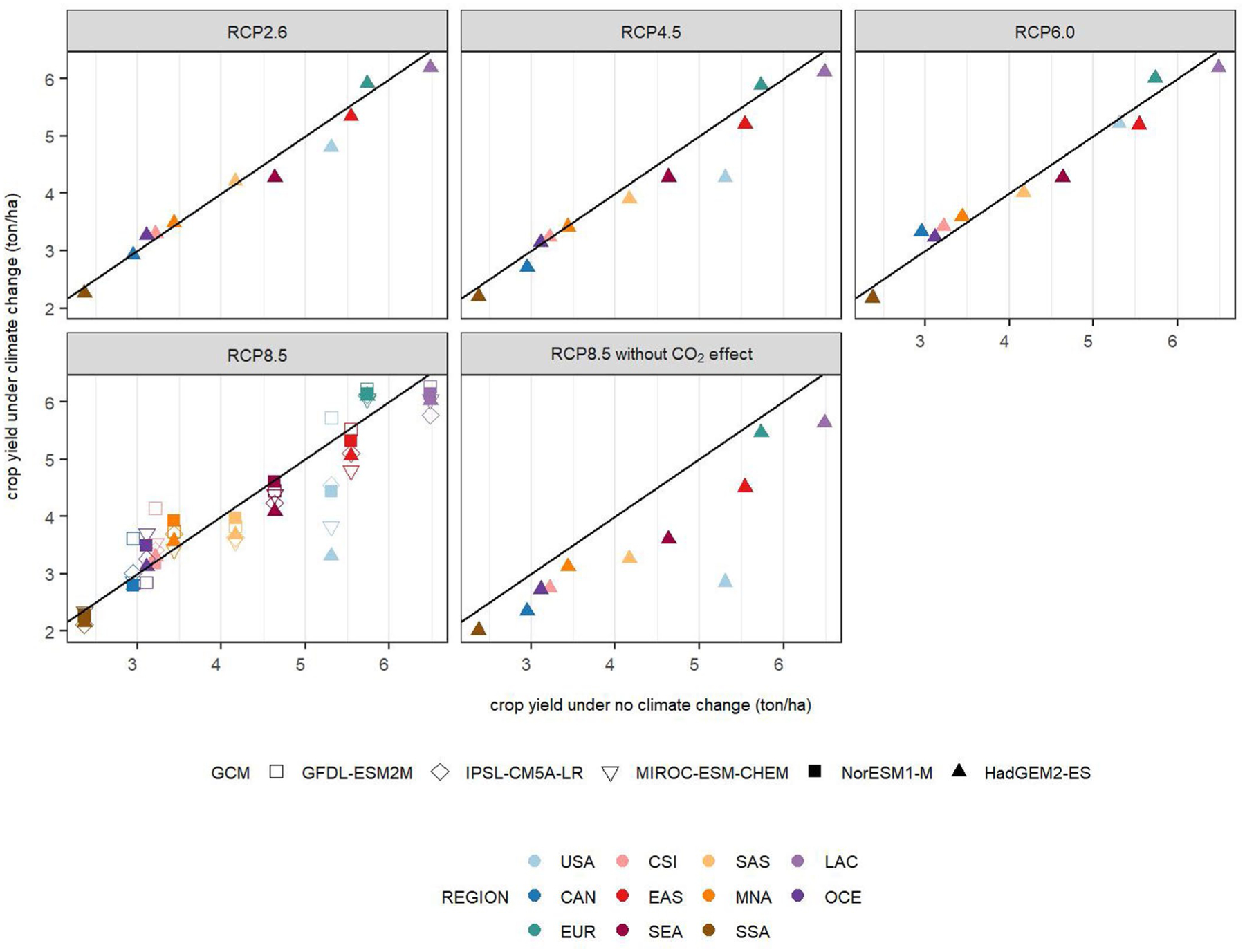
Yields in ton dry matter per ha. The x-axis indicates the crop yield under no climate change and y-axis the crop yield under climate change for different RCP × GCM combinations without market feedback and adaptation measures. Under no climate change yields are determined by base year yield and assumptions on technological development over time, under climate change an additional climate impact shifter is applied. Points above the black line indicate an increase in crop yield, points below a decrease in crop yield.

Extended Data Fig. 2 |. Impact of climate change on average crop yield after supply-side adaptation in each region by 2050 as projected by GLOBIOM.

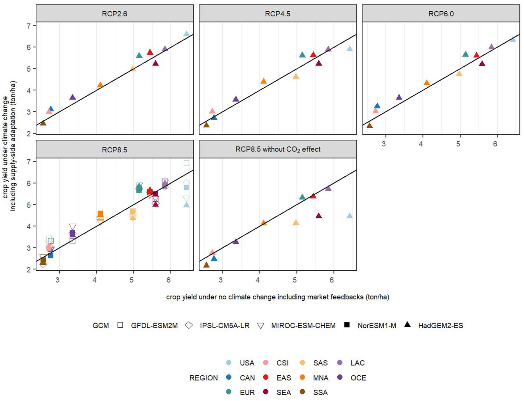
Yields in ton dry matter per ha. The x-axis indicates the crop yield under no climate change and y-axis the crop yield under climate change for different RCP × GCM combinations with GLOBIOM market feedback and supply-side adaptation (changes in management system and reallocation of production across spatial units in response to price changes). Points above the black line indicate an increase in crop yield, points below a decrease in crop yield.

Extended Data Fig. 3 |. Net agricultural trade of baseline net importing regions in 2050 under trade and climate change scenarios.

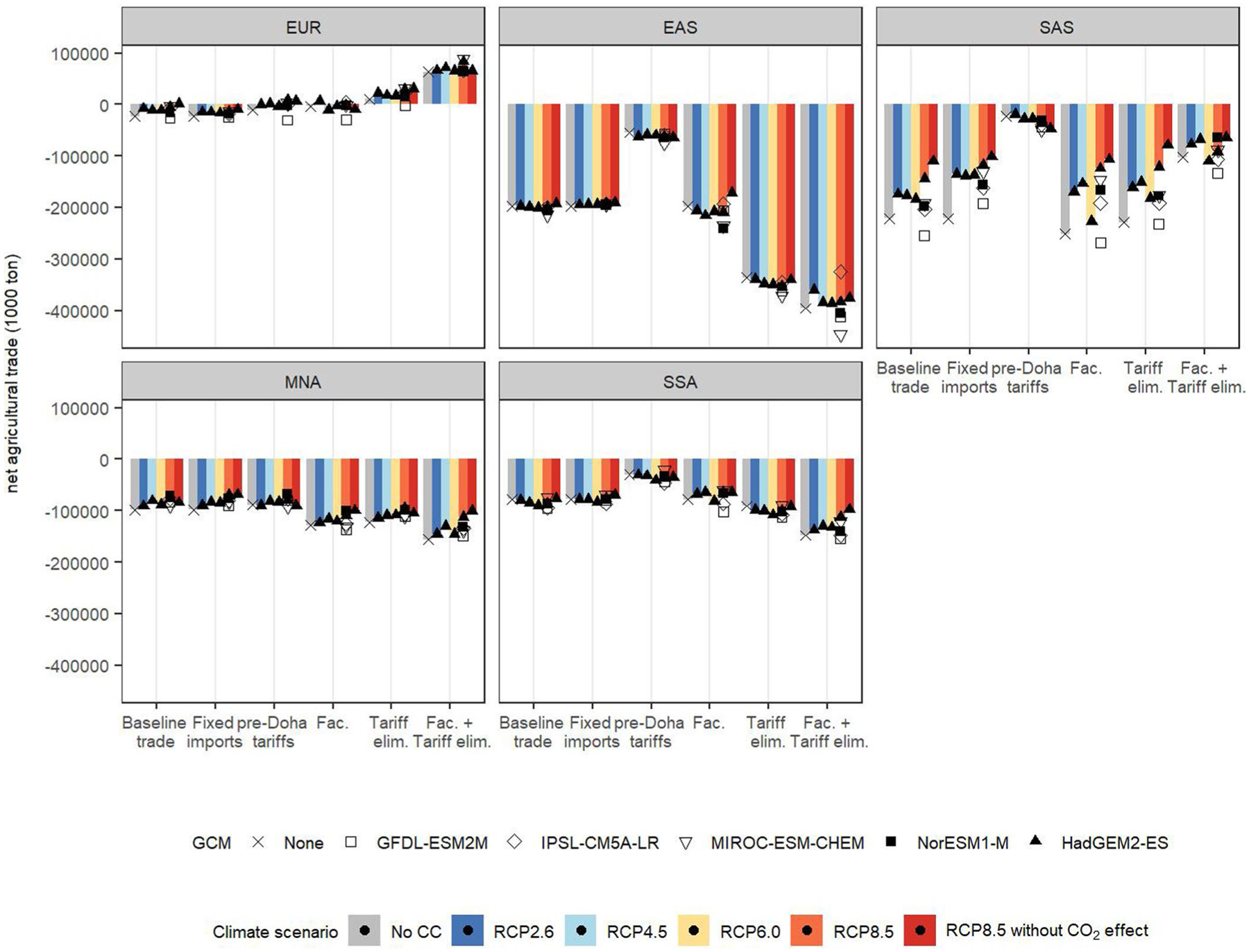
Net agricultural trade in ton dry matter. Fac. = Facilitation, Tariff elim. = Tariff elimination.

Extended Data Fig. 4 |. Net agricultural trade of baseline net exporting regions in 2050 under trade and climate change scenarios.

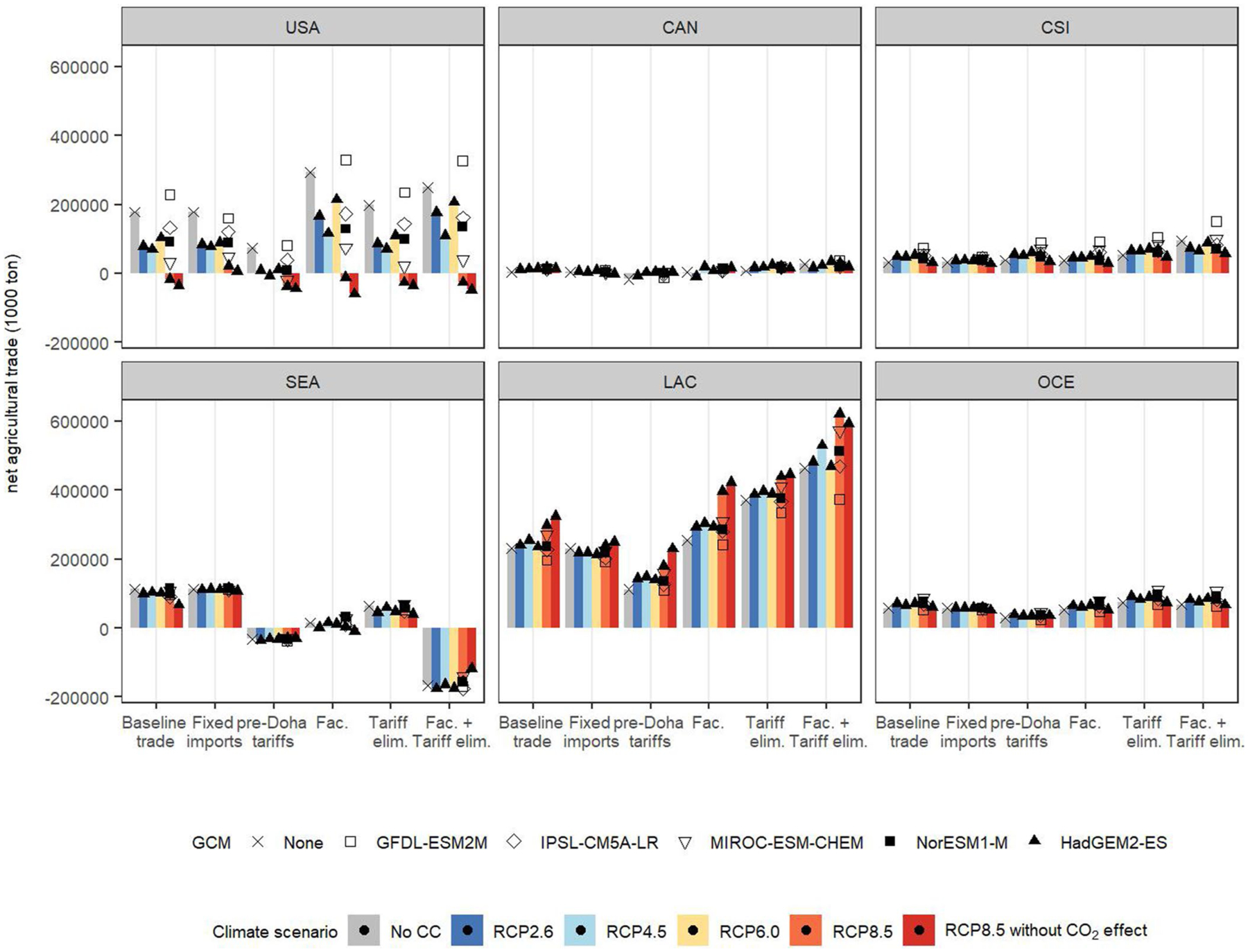
Net agricultural trade in ton dry matter. Fac. = Facilitation, Tariff elim. = Tariff elimination.

Extended Data Fig. 5 |. Change in agricultural prices of baseline net importing regions in 2050 under trade and climate change scenarios compared to SSP2 baseline.

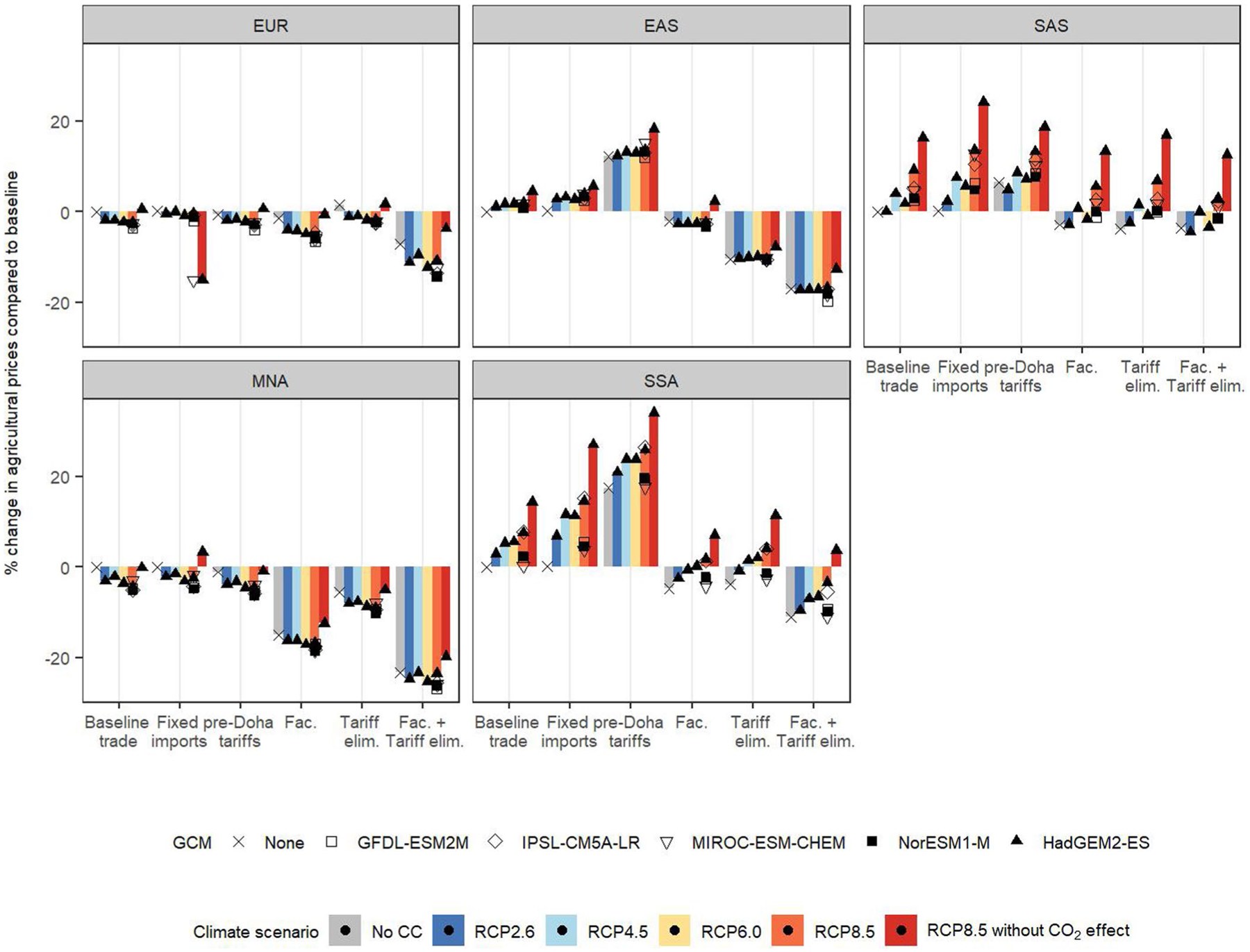
Fac. = Facilitation, Tariff elim. = Tariff elimination.

Extended Data Fig. 6 |. Change in agricultural prices of baseline net exporting regions in 2050 under trade and climate change scenarios compared to SSP2 baseline.

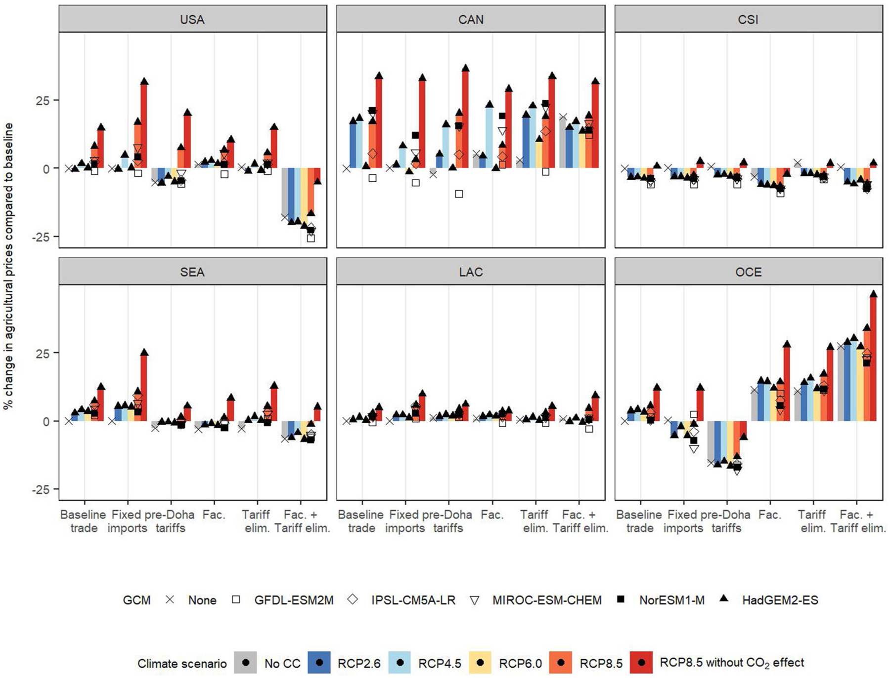
Fac. = Facilitation, Tariff elim. = Tariff elimination.

Extended Data Fig. 7 |. Change in population at risk of hunger in 2050 in hunger-affected regions under climate change and trade scenarios compared to SSP2 baseline.

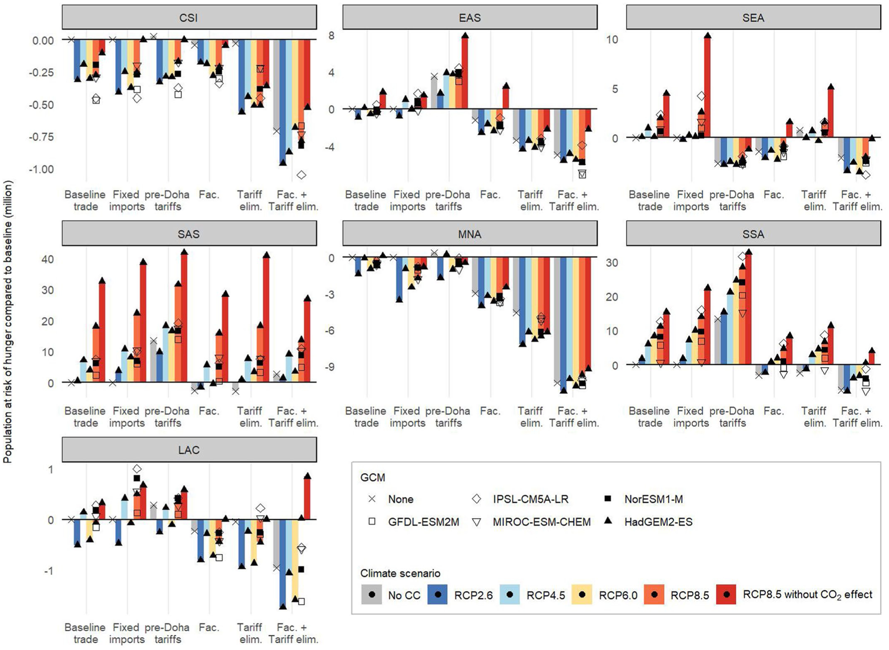
Fac. = Facilitation, Tariff elim. = Tariff elimination. The estimated risk of hunger in the other world regions is zero (CAN, EUR) or very low (OCE, USA).

Extended Data Fig. 8 |. Plot of the fitted linear response of population at risk of hunger (million) to climate-induced crop yield change for different values of trade costs (1^st decile, median, 9^th decile).

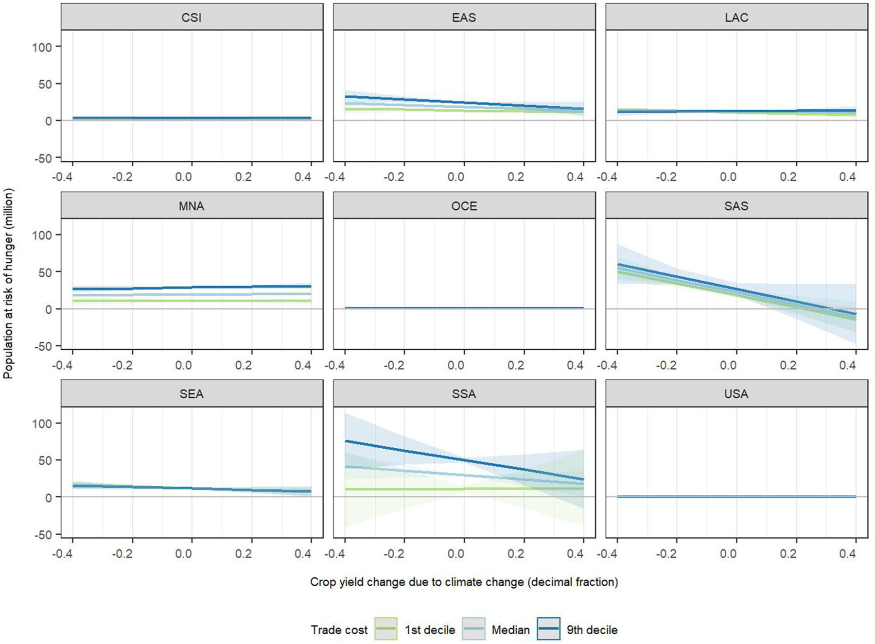
Shaded areas indicate prediction intervals. Prediction based on an OLS estimation of a regional level linear regression of the impact of crop yield change, trade costs and their interaction on population at risk of hunger. Regression results are shown in Supplementary Table 3 and the regression model is described in Method.

Extended Data Fig. 9 |. Share of production volume that each region represents of total world production for corn, rice, soya and wheat in the SSP2 baseline in 2050.

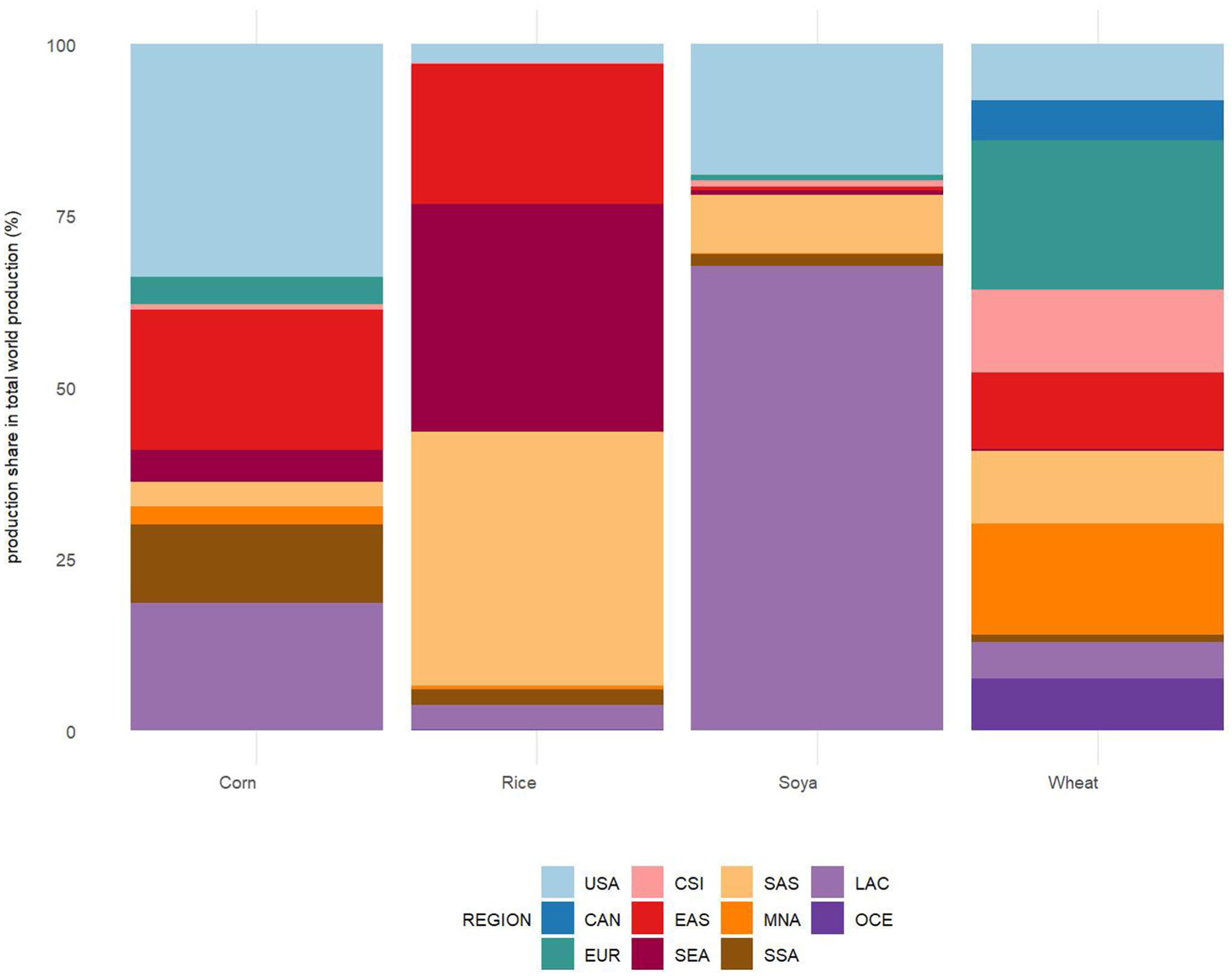
The projected total world production by 2050 in the SSP2 baseline is 1213 Mt for corn, 884 Mt for rice, 309 Mt for soya and 794 Mt for wheat.

Extended Data Fig. 10 |. Net trade (1000 ton) in East asia (EaS), Middle East and North africa (MNa), South asia (SaS) and Sub-Saharan africa (SSa) for corn, rice, soya and wheat under climate change and trade scenarios in 2050.

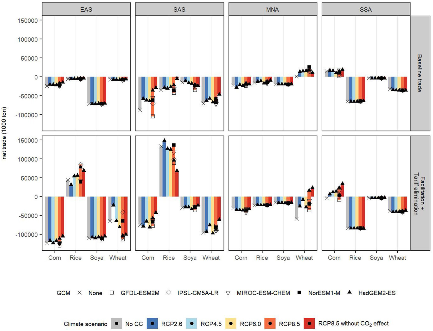
Net agricultural trade in ton dry matter. Values above zero indicate net exports, negative values indicate net imports.

References

- 1.FAO, IFAD, UNICEF, WFP & WHO The State of Food Security and Nutrition in the World 2018. Building Climate Resilience for Food Security and Nutrition (FAO, 2018). [Google Scholar]
- 2.Nelson GC et al. Climate change effects on agriculture: economic responses to biophysical shocks. Proc. Natl Acad. Sci. USA 111, 3274–3279 (2014). [DOI] [PMC free article] [PubMed] [Google Scholar]
- 3.2019 Global Food Policy Report (IFPRI, 2019). [Google Scholar]
- 4.Hoegh-Guldberg O et al. in Special Report on Global Warming of 1.5 °C (eds Masson-Delmotte V. et al.) Ch. 3 (WMO, 2018). [Google Scholar]
- 5.Hertel TW Climate Change, Agricultural Trade and Global Food Security. The State of Agricultural Commodity Markets (SOCO) 2018: Background Paper 9 (FAO, 2018). [Google Scholar]
- 6.Huang H, von Lampe M & van Tongeren F Climate change and trade in agriculture. Food Policy 36, S9–S13 (2011). [Google Scholar]
- 7.Brown ME et al. Do markets and trade help or hurt the global food system adapt to climate change? Food Policy 68, 154–159 (2017). [Google Scholar]
- 8.Rosenzweig C et al. Assessing agricultural risks of climate change in the 21st century in a global gridded crop model intercomparison. Proc. Natl Acad. Sci. USA 111, 3268–3273 (2014). [DOI] [PMC free article] [PubMed] [Google Scholar]
- 9.Stevanović M et al. The impact of high-end climate change on agricultural welfare. Sci. Adv 24, e1501452 (2016). [DOI] [PMC free article] [PubMed] [Google Scholar]
- 10.Wiebe K et al. Climate Change impacts on agriculture in 2050 under a range of plausible socioeconomic and emissions scenarios. Environ. Res. Lett 10, 085010 (2015). [Google Scholar]
- 11.Gouel C & Laborde D The Crucial Role of International Trade in Adaptation to Climate Change Working Paper No. 25221 (National Bureau of Economic Research, 2018). [Google Scholar]
- 12.Costinot A, Donaldson D & Smith C Evolving comparative advantage and the impact of climate change in agricultural markets: evidence from 1.7 million fields around the world. J. Polit. Econ 124, 205–248 (2016). [Google Scholar]
- 13.Baldos ULC & Hertel TW The role of international trade in managing food security risks from climate change. Food Secur. 7, 275–290 (2015). [Google Scholar]
- 14.Cui HD, Kuiper M, van Meijl H & Tabeau A Climate Change and Global Market integration: Implications for Global Economic Activities, Agricultural Commodities, and Food Security. The State of Agricultural Commodity Markets (SOCO) 2018: Background Paper (FAO, 2018). [Google Scholar]
- 15.Lobell DB Climate change adaptation in crop production: beware of illusions. Glob. Food Sec 3, 72–76 (2014). [Google Scholar]
- 16.Moore FC, Baldos ULC & Hertel T Economic impacts of climate change on agriculture: a comparison of process-based and statistical yield models. Environ. Res. Lett 12, 065008 (2017). [Google Scholar]
- 17.Zimmermann A, Benda J, Webber H & Jafari Y Trade, Food Security and Climate Change: Conceptual Linkages and Policy Implications Background Paper for The State of Agricultural Commodity Markets (SOCO) 2018 (FAO, 2018). [Google Scholar]
- 18.Hoekman B & Nicita A Trade policy, trade costs, and developing country trade. World Dev. 39, 2069–2079 (2011). [Google Scholar]
- 19.Disdier AC & van Tongeren F Non-tariff measures in agri-food trade: what do the data tell us? Evidence from a cluster analysis on OECD imports. Appl. Econ. Perspect. Policy 32, 436–455 (2010). [Google Scholar]
- 20.Bureau J, Guimbard H & Jean S Agricultural trade liberalisation in the 21st century: has it done the business? J. Agric. Econ 70, 3–25 (2018). [Google Scholar]
- 21.Arvis JF, Duval Y, Shepherd B, Utoktham C & Raj A Trade costs in the developing world: 1996–2010. World Trade Rev. 15, 451–474 (2016). [Google Scholar]
- 22.Mosnier A et al. Global food markets, trade and the cost of climate change adaptation. Food Secur. 6, 29–44 (2014). [Google Scholar]
- 23.Leclère D et al. Climate Change induced transformations of agricultural systems: insights from a global model. Environ. Res. Lett 9, 124018 (2014). [Google Scholar]
- 24.Baker J et al. Evaluating the effects of climate change on US agricultural systems: sensitivity to regional impact and trade expansion scenarios. Environ. Res. Lett 13, 064019 (2018). [DOI] [PMC free article] [PubMed] [Google Scholar]
- 25.Havlík P et al. Climate Change Impacts and Mitigation in the Developing World, An Integrated Assessment of the Agriculture and Forestry Sectors. Background Paper for the World Bank Report: “Shock Waves: Managing the Impacts of Climate Change on Poverty.” Policy Research Working Paper WPS7477 (The World Bank, 2015). [Google Scholar]
- 26.IPCC Climate Change 2014: Synthesis Report (eds Core Writing Team, Pachauri RK & Meyer LA) (IPCC, 2014). [Google Scholar]
- 27.Fricko O et al. The marker quantification of the Shared Socioeconomic Pathway 2: A middle-of-the-road scenario for the 21st century. Glob. Environ. Change 42, 251–267 (2017). [Google Scholar]
- 28.Bouët A & Laborde Debucquet D in Food Price Volatility and Its Implications for Food Security and Policy (eds Kalkuhl M et al.) 167–179 (Springer, 2016); 10.1007/978-3-319-28201-5_8 [DOI] [Google Scholar]
- 29.Kornher L Maize Markets in Eastern and Southern Africa (ESA) in the Context of Climate Change. The State of Agricultural Commodity Markets (SOCO) 2018: Background Paper (FAO, 2018). [Google Scholar]
- 30.Glauber J, Laborde D, Martin W & Vos R COVID-19: Trade Restrictions are Worst Possible Response to Safeguard Food Security (IFPRI, 2020); https://www.ifpri.org/blog/covid-19-trade-restrictions-are-worst-possible-responsesafeguard-food-security [Google Scholar]
- 31.Sulser T & Dunston S COVID-19-Related Trade Restrictions on Rice and Wheat Could Drive Up Prices and Increase Hunger (IFPRI, 2020); https://www.ifpri.org/blog/covid-19-related-trade-restrictions-rice-and-wheat-could-drive-prices-and-increase-hunger [Google Scholar]
- 32.Dithmer J & Abdulai A Does trade openness contribute to food security? A dynamic panel analysis. Food Policy 69, 218–230 (2017). [Google Scholar]
- 33.Bureau JC & Swinnen J EU policies and global food security. Glob. Food Sec 16, 106–115 (2018). [Google Scholar]
- 34.Porter JR et al. Food security and food production systems in Climate Change 2014: Impacts, Adaptation, and Vulnerability (eds Field CB et al.) 485–533 (Cambridge Univ. Press, 2014). [Google Scholar]
- 35.Swinnen J & Squicciarini P Mixed messages on prices and food security. Science 335, 405–406 (2012). [DOI] [PubMed] [Google Scholar]
- 36.Calderon C, Cantu C & Chuhan-Pole P Infrastructure Development in Sub-Saharan Africa: A Scorecard Policy Research Working Paper WPS8425 (The World Bank, 2018). [Google Scholar]
- 37.African Economic Outlook 2018 (African Development Bank, 2018). [Google Scholar]
- 38.Mosnier A Tracking Indirect Effects of Climate Change Mitigation and Adaptation Strategies in Agriculture and Land Use Change With a Bottom-Up Global Partial Equilibrium Model (Univ. Natural Resources and Life Sciences (BOKU), 2014). [Google Scholar]
- 39.Valin H et al. The future of food demand: understanding differences in global economic models. Agric. Econ 45, 51–67 (2014). [Google Scholar]
- 40.Herrero M et al. Biomass use, production, feed efficiencies, and greenhouse gas emissions from global livestock systems. Proc. Natl Acad. Sci. USA 110, 20888–20893 (2013). [DOI] [PMC free article] [PubMed] [Google Scholar]
- 41.Forsell N et al. Assessing the INDCs’ land use, land use change, and forest emission projections. Carbon Balance Manag. 11, 26 (2016). [DOI] [PMC free article] [PubMed] [Google Scholar]
- 42.Havlík P et al. Global land-use implications of first and second generation biofuel targets. Energy Policy 39, 5690–5702 (2011). [Google Scholar]
- 43.Havlik P et al. Climate change mitigation through livestock system transitions. Proc. Natl Acad. Sci. USA 111, 3709–3714 (2014). [DOI] [PMC free article] [PubMed] [Google Scholar]
- 44.Takayama T & Judge GG Spatial and Temporal Price and Allocation Models (North-Holland Publishing Company, 1971). [Google Scholar]
- 45.Gaulier G & Zignago S BACI: International Trade Database at the Product-Level. The 1994–2007 Version Working Paper 1–35 (CEPII, 2010); 10.2139/ssrn.1994500 [DOI] [Google Scholar]
- 46.Bouët A, Decreux Y, Fontagné L, Jean S & Laborde D Assessing applied protection across the world. Rev. Int. Econ 16, 850–863 (2008). [Google Scholar]
- 47.Hummels D Toward a Geography of Trade Costs (Purdue University, 2001). [Google Scholar]
- 48.Bouët A, Decreux Y, Fontagné L, Jean S & Laborde D A Consistent, Ad-Valorem Equivalent Measure of Applied Protection Across the World: The MAcMap-HS6 Database Working Papers 2004–22 (CEPII Research Center, 2004); http://cepii.fr/PDF_PUB/wp/2004/wp2004-22.pdf [Google Scholar]
- 49.Guimbard H, Jean S, Mimouni M & Pichot X MAcMap-HS6 2007, an Exhaustive and Consistent Measure of Applied Protection in 2007. J. Int. Econ 130, 99–122 (2012). [Google Scholar]
- 50.Hummels D Transportation costs and international trade in the second era of globalization. J. Econ. Perspect 21, 131–154 (2007). [Google Scholar]
- 51.Hasegawa T et al. Consequence of climate mitigation on the risk of hunger. Environ. Sci. Technol 49, 7245–7253 (2015). [DOI] [PubMed] [Google Scholar]
- 52.Hasegawa T et al. Risk of increased food insecurity under stringent global climate change mitigation policy. Nat. Clim. Change 8, 699–703 (2018). [Google Scholar]
- 53.Hasegawa T, Fujimori S, Takahashi K & Masui T Scenarios for the risk of hunger in the twenty-first century using Shared Socioeconomic Pathways. Environ. Res. Lett 10, 014010 (2015). [Google Scholar]
- 54.Global Spatially-Disaggregated Crop Production Statistics Data for 2000 Version 3.0.7 (IFPRI, 2019); 10.7910/DVN/A50I2T [DOI] [Google Scholar]
- 55.Moore FC, Baldos U, Hertel T & Diaz D New science of climate change impacts on agriculture implies higher social cost of carbon. Nat. Commun 8, 1607 (2017). [DOI] [PMC free article] [PubMed] [Google Scholar]
- 56.Costinot A, Donaldson D & Komunjer I What goods do countries trade? A quantitative exploration of Ricardo’s ideas. Rev. Econ. Stud 79, 581–608 (2012). [Google Scholar]
- 57.Clapp J Food Security and International Trade: Unpacking disputed narratives. The State of Agricultural Commodity Markets 2015–2016 (FAO, 2015). [Google Scholar]
- 58.Warszawski L et al. The inter-sectoral impact model intercomparison project (ISI-MIP): project framework. Proc. Natl Acad. Sci. USA 111, 3228–3232 (2014). [DOI] [PMC free article] [PubMed] [Google Scholar]
- 59.van Vuuren DP et al. The representative concentration pathways: an overview. Climatic Change 109, 5–31 (2011). [Google Scholar]
- 60.Martin GM et al. The HadGEM2 family of Met Office unified model climate configurations. Geosci. Model Dev 4, 723–757 (2011). [Google Scholar]
- 61.Collins WJ et al. Development and evaluation of an Earth-system model—HadGEM2. Geosci. Model Dev 4, 1051–1075 (2011). [Google Scholar]
- 62.Dunne JP et al. GFDL’s ESM2 global coupled climate-carbon Earth system models. part I: physical formulation and baseline simulation characteristics. J. Clim 25, 6646–6665 (2012). [Google Scholar]
- 63.Dufresne JL et al. Climate change projections using the IPSL-CM5 Earth system model: from CMIP3 to CMIP5. Clim. Dyn 40, 2123–2165 (2013). [Google Scholar]
- 64.Watanabe S et al. MIROC-ESM 2010: model description and basic results of CMIP5–20c3m experiments. Geosci. Model Dev 4, 845–872 (2011). [Google Scholar]
- 65.Bentsen M et al. The Norwegian Earth System Model, NorESM1-M—part 1: description and basic evaluation of the physical climate. Geosci. Model Dev 6, 687–720 (2013). [Google Scholar]
- 66.Moïsé E & Sorescu S Trade Facilitation Indicators—The Potential Impact of Trade Facilitation on Developing Countries’ Trade OECD Trade Policy Papers No. 144 (OECD Publishing, 2013). [Google Scholar]
- 67.Non-Tariff Measures to Trade: Economic and Policy Issues for Developing Countries (UNCTAD, 2013). [Google Scholar]
- 68.Minor PJ Time as a Barrier to Trade: A GTAP Database of Ad Valorem Trade Time Costs 2nd edn (ImpactEcon, 2013). [Google Scholar]
- 69.Petri PA & Plummer MG The Economic Effects of the Trans-Pacific Partnership: New Estimates Working Paper 16–2 (Peterson Institute for International Economics, 2016). [Google Scholar]
- 70.Balistreri EJ, Maliszewska M, Osorio-Rodarte I, Tarr DG & Yonezawa H Poverty, welfare and income distribution implications of reducing trade costs through deep integration in eastern and Southern Africa. J. Afr. Econ 27, 172–200 (2018). [Google Scholar]
- 71.Anderson K & Martin W Agricultural Trade Reform and the Doha Development Agenda (The World Bank and Palgrave Macmillan, 2006). [Google Scholar]
- 72.Riahi K et al. The Shared Socioeconomic Pathways and their energy, land use, and greenhouse gas emissions implications: an overview. Glob. Environ. Change 42, 153–168 (2017). [Google Scholar]
- 73.Valin H et al. Agricultural productivity and greenhouse gas emissions: trade-offs or synergies between mitigation and food security? Environ. Res. Lett 8, 035019 (2013). [Google Scholar]
- 74.Long JS & Ervin LH Using heteroscedasticity consistent standard errors in the linear regression model. Am. Stat 54, 217–224 (2000). [Google Scholar]
Associated Data
This section collects any data citations, data availability statements, or supplementary materials included in this article.
Supplementary Materials
Data Availability Statement