Exploring Uncertainty Measures in Bayesian Deep Attentive Neural Networks for Prostate Zonal Segmentation

Abstract

Automatic segmentation of prostatic zones on multiparametric MRI (mpMRI) can improve the diagnostic workflow of prostate cancer. We designed a spatial attentive Bayesian deep learning network for the automatic segmentation of the peripheral zone (PZ) and transition zone (TZ) of the prostate with uncertainty estimation. The proposed method was evaluated by using internal and external independent testing datasets, and overall uncertainties of the proposed model were calculated at different prostate locations (apex, middle, and base). The study cohort included 351 MRI scans, of which 304 scans were retrieved from a de-identified publicly available datasets (PROSTATEX) and 47 scans were extracted from a large U.S. tertiary referral center (external testing dataset; ETD)). All the PZ and TZ contours were drawn by research fellows under the supervision of expert genitourinary radiologists. Within the PROSTATEX dataset, 259 and 45 patients (internal testing dataset; ITD) were used to develop and validate the model. Then, the model was tested independently using the ETD only. The segmentation performance was evaluated using the Dice Similarity Coefficient (DSC). For PZ and TZ segmentation, the proposed method achieved mean DSCs of 0.80±0.05 and 0.89±0.04 on ITD, as well as 0.79±0.06 and 0.87±0.07 on ETD. For both PZ and TZ, there was no significant difference between ITD and ETD for the proposed method. This DL-based method enabled the accuracy of the PZ and TZ segmentation, which outperformed the state-of-art methods (Deeplab V3+, Attention U-Net, R2U-Net, USE-Net and U-Net). We observed that segmentation uncertainty peaked at the junction between PZ, TZ and AFS. Also, the overall uncertainties were highly consistent with the actual model performance between PZ and TZ at three clinically relevant locations of the prostate.

I. INTRODUCTION

Prostate cancer (PCa) is the most common solid organ malignancy and is among the most common causes of cancer-related death among men in the United States [1]. Multiparametric MRI (mpMRI) is the most widely available non-invasive and sensitive tool for the detection of clinically significant PCa (csPCa), 70% and 30% of which are located in the peripheral zone (PZ) and transition zone (TZ) respectively [2], [3]. The clinical reporting of mpMRI relies on a qualitative expert consensus-based structured reporting scheme (Prostate Imaging-Reporting and Data System (PI-RADS)). The interpretation is based primarily on diffusion-weighted imaging (DWI) in the peripheral zone (PZ) and T2-weighted (T2w) imaging in the transitional zone (TZ) since csPCa lesions have different primary imaging features [2], [3].

Accurate segmentation of PZ and TZ within the 3T mpMRI is essential for localization and staging of csPCa to enable MR targeted biopsy and guide and plan further therapy such as radiation, surgery, and focal ablation [4]. Segmentation of the prostate zones on mpMRI is typically done manually, which can be time-consuming and sensitive to readers’ experience, resulting in significant intra- and inter-reader variability [5]. Automated segmentation of prostatic zones (ASPZ) is reproducible and beneficial for consistent location assignment of PCa lesions [6]. ASPZ also enables automated quantitative imaging feature extraction related to prostate zones and can be used as a pre-processing step to improve the computer-aided diagnosis (CAD) of PCa [7].

ASPZ was previously proposed by the atlas-based method [8]. Later, Zabihollahy et al. [9] proposed a U-Net-based method for ASPZ. Clark et al. [10] developed a staged deep learning architecture, which incorporated a classification into U-Net, to segment the whole prostate gland and TZ. However, the U-Net-based segmentation sometimes resulted in inconsistent performance because the anatomic structure of the prostate can be less distinguishable, and the boundaries between PZ and TZ may distort semantic features [5]. Liu et al. [5] recently improved the encoder of the U-Net by using the residual neural network, ResNet50 [11], followed by feature pyramid attention to help capture the information at multiple scales. Furthermore, Rundo et al. [12] proposed an attentive deep learning network for ASPZ via incorporating the squeeze and excitation (SE) blocks into U-Net. SE adaptively recalibrated the channel-wise features to potentially improve inconsistencies in the segmentation performance.

Moreover, segmentation outcomes from ASPZ are typically deterministic; there is a lack of knowledge on the confidence of the model [13]. Providing uncertainties of the model can improve the overall segmentation workflow since it easily allows refining uncertain cases by human experts [13]. The uncertainty can be estimated by the Bayesian deep learning model, which not only produces predictions but also provides the uncertainty estimations for each pixel. This can be done by adopting probability distributions of weights rather than the deterministic weights of the model.

In this study, we propose an ASPZ with an estimation of pixel-wise uncertainties using a spatial attentive Bayesian deep learning network. Different from Rundo et al. [12], we adopt a spatial attentive module (SAM), which models the long-range spatial dependencies between PZ and TZ by calculating the pixel level response from the image [14]. The proposed model incorporates four sub-networks, including SAM, an improved ResNet50 with dropout, a multiple-scaled feature pyramid attention module (MFPA) [5], and a decoder. The SAM forces the entire network focusing on specific regions that have more abundant semantic information related to prostatic zones. We use the improved ResNet50 to handle the heterogeneous prostate anatomy with semantic features. The MFPA is designed to enhance the multi-scale feature capturing. Finally, the spatial resolution is recovered by the decoder. We also implement the Bayesian model through both training the proposed model with dropout and Monte Carlo (MC) samples of the predictions during the inference, inspired by prior work by Gal and Ghahramani [15]. The dropout can be regarded as using Bernoulli’s random variables to sample the model weights [15].

We evaluate the proposed model’s performance using internal and external testing datasets and compared it with previously developed ASPZ methods. The segmentation performance is compared to investigate the discrepancy between two MRI datasets. The importance of each individual module within the proposed method is also examined. Finally, the overall prostate zonal segmentation at apex, middle, and base slices are computed to illustrate the uncertainty of segmentation at different positions of the prostate.

II. MATERIALS

This study was carried out in compliance with the United States Health Insurance Portability and Accountability Act (HIPAA) of 1996 with approval by the local institutional review board (IRB). The MRI datasets were acquired from two sources. For model development and internal testing (n = 259 and n = 45)—internal testing dataset (ITD)—we used the Cancer Imaging Archive (TCIA) data from the SPIE-AAPM-NCI PROSTATE X (PROSTATE X) challenge. [16] For independent model testing, we used an external testing dataset (ETD) (n = 47; age 45 to 73 years and weight 68 to 113 kg) retrieved from our tertiary academic medical center. For the ETD, the pre-operative MRI scans, which were acquired between October 2017 and December 2018 using one of the three 3T MRI scanners (Skyra (n = 39), Prisma (n = 1), and Vida (n = 7); (Siemens Healthineers, Erlangen, Germany)) were collated.

For both ITD and ETD data, both PZ and TZ were contoured using OsiriX (Pixmeo SARL, Bernex, Switzerland) by MRI research fellows. Then, two genitourinary radiologists (10–19 years of post-fellowship experience interpreting over 10,000 prostate MRI) cross-checked the contours. The axial T2 TSE (turbo spin-echo) MRI sequence was used for both ITD and ETD segmentation (Table I). Prior to the training and testing, all the images in both datasets were normalized to an interval of [0,1] and were also resampled to the common in-plane resolution (0.5 × 0.5 mm).

TABLE I.

Detailed T2w TSE protocols from two MRI datasets.

Datasets	Internal Testing dataset (ITD)	External Testing dataset (ETD)
Spatial Resolution	0.5×0.5×3.0mm3	0.65×0.65×3.6mm3
Matrix Size	380×380	320×320
Flip angle	160°	160°
Repetition Time/Echo Time	5660 ms / 104 ms	4000 ms / 109 ms
Field-of-View	190×190 mm2	208×208 mm2

III. METHODS

A. PROPOSED MODEL FOR AUTOMATIC PROSTATIC ZONAL SEGMENTATION

The overall workflow of the proposed network is shown in Figure 1, which consists of four sub-networks. By joining the four sub-networks together, a fully end-to-end prostatic zonal segmentation workflow was formed. Both PZ and TZ segmentations were done simultaneously using a single network.

Fig. 1.

A whole workflow of the proposed model. Input is a 2D T2w MRI slice, and output is a segmentation mask, which has the PZ and TZ segmentation result (Gray and white colors indicate PZ and TZ, respectively), and a pixel-wise uncertainty map (yellow pixel indicates large uncertainty and blue indicates low uncertainty). There are four sub-networks in the network, which are (a) spatial attention module (SAM), (b) improved ResNet50, (c) multiple-scaled feature pyramid attention (FPA), and (d) decoder.

1). SPATIAL ATTENTIVE MODULE (SAM):

Inspired by Wang et al. [14], the SAM was designed to make the network intelligently pay attention to the regions, which had more semantic features associated with PZ and TZ (shown in Figure 1.a).

Inside the images, there existed some spatial dependencies of PZ and TZ pixels. For instance, TZ was always surrounded by PZ in the bottom of the prostate, and the urinary bladder region was always above PZ and TZ in the image and TZ was usually in the image center. SAM helped the network to model such spatial dependent information through global features. Specifically, the response at each pixel was computed by considering all the pixels in the image. Higher priorities were then adaptively assigned to the pixels, which had more informative semantic features.

Detailed processes regarding spatial attention are shown in the left bottom of Figure 1. After going through a convolution layer and reshaping, three kinds of vectors - query vector α(x),key vector β (x) and representative vector g (x), were formed. Then, we performed the matrix multiplication between the transpose of the query vector and the key vector, and after that, we applied a soft-max layer to compute the weight matrix which models the spatial relationship between any two pixels of the features. Next, we again performed a matrix multiplication between the weight matrix and the representative vector and reshaped the result to the size of original features. These processes can be formulated by:

$$\text{y}=\text{softmax}(\alpha {(x))}^T*(\beta (x)))*g(x)$$ (1)

where x and y represent the raw image and attentive map of the raw image, respectively. ^∗ means matrix multiplication. Finally, an element-wise sum operation between the result above and the original features was performed to obtain the final result which reflected the long-range dependencies.

2). IMPROVED RESNET50 WITH DROPOUT:

Improved ResNet50 (shown in Figure 1.b) was served as the bone structure of the network. ResNet50 in this paper was improved by the following three steps, which followed the methods of Liu et al. [5]. First, the initial max-pool was removed since it was proved to compromise the performance of segmentation. Bottleneck block at stride one as the first block in the 4^th layer was replaced with the regular block. Then, we used the dilated bottleneck to serve as the second block in the 4^th layer so as to minimize the potential loss to the spatial information. Finally, the dropout layer was inserted after each block within the improved ResNet50 to transform the current neural network to the bayesian neural network [17].

3). MULTI-SCALED FEATURE PYRAMID ATTENTION (MFPA):

Feature pyramid attention (FPA) module (shown in the bottom right of Figure 1) was applied after each layer within Resnet50 to help capture the features from the multiple scales. Next, feature maps after each FPA were then upsampled to the same size and then concatenated in the decoder.

4). DECODER:

The decoder (Figure 1.d) was used to recover feature maps’ spatial resolution. In the decoder, the total features calculated in the 3) went through two 3 × 3 convolutional layers and one 1 × 1 convolutional layer, followed by an up-sampling (by a factor of 4). In the end, the multi-class softmax classifier was performed for the simultaneous segmentation of TZ and PZ.

B. UNCERTAINTY ESTIMATION FOR PROSTATE ZONAL SEGMENTATION

Figure 1 shows the uncertainty estimation workflow by the proposed method. Monte Carlo dropout [15] was served as the method for approximate inference.

Usually, a posterior distribution p(W|X, Y ) placed over weights W of the neural network is computed to capture the uncertainty in the model, where X is the training samples, and Y is the corresponding ground truth labels of prostate zones [18]. However, it is intractable to compute the posterior. The posterior can be approximated by the variational distribution q(W), which minimizes the Kullback-Leibler (KL) divergence between the actual posterior and the variational distribution: $\text{KL}(q(W))\mid \mid p(W\mid X,Y))$ [18]. It is noted that performing dropout on a hidden layer is equivalent to placing the variational distribution – Bernoulli distribution over the weights of that layer [15]. Also, the effect of minimizing the cross-entropy loss is the same as the minimization of the KL-divergence. Therefore, training with dropout allows the approximate inference. These dropouts are also required to be kept active during the testing. As the dropout is the same as placing a Bernoulli distribution over the network weights, the sample from a dropout network’s outputs can be used to approximate the posterior. A Monte Carlo sample from the posterior distribution is produced by performing a stochastic forward pass through a trained dropout network. There are two types of uncertainties: epistemic uncertainty — caused by the ineptitude of the model because of the lack of training data; aleatoric uncertainty — caused by the noisy measurements in the data [15]. Epistemic uncertainty can be mitigated by increasing the training samples. Aleatoric uncertainty can be restrained by increasing the sensor precision. Aleatoric uncertainty occurs during measuring the inherent noise in the samples and is reflected in the uncertainty over the model’s parameters [19]. A model with the precise set of parameters will lower down the aleatoric uncertainty [19]. The combination of aleatoric and epistemic uncertainty forms the predictive uncertainty [18]. In this paper, we focused on the exploring of predictive uncertainty for the prostate zonal segmentation, which can be measured by the entropy of the predictive distribution [18], [19] and is formulated as:

$$-\sum _{c=1}^C\frac{1}{T}\sum _{t=1}^{T}p\left(y=c\mid x,w_t\right))\log \left(\frac{1}{T}\sum _{t=1}^{T}p\left(y=c\mid x,w_t\right)\right)$$ (2)

where y is the output variable, T is the number of stochastic forward passes (50 was chosen is the experiments (Figure 1)), C is the number of classes (C=3, for background, PZ and TZ), p (y = c|x, w_t ) is the soft-max probability of input x being in class c, w_t represents model’s parameters on the t_th forward pass.

C. AVERAGE UNCERTAINTY MAPS FOR THE PROSTATE ZONAL SEGMENTATION

The average uncertainty map tells the overall zonal uncertainty in different positions on the prostate image. Figure 2 shows the processes of obtaining the average uncertainty map. In order to obtain the average uncertainty map at the prostate apex, middle portion, and base, three template prostate images at the three sections were chosen by a radiologist after inspecting all the prostate images. Next, for each prostate section, zonal boundary points on non-template prostate images (sample images) were then registered to those on the prostate template image within the section using a non-rigid coherent point drift method (CPD) [20]. Within non-rigid CPD, alignment of two-point sets was thought of as a probability density estimation problem where one point set serves as the centroids of the gaussian mixture model (GMM), and the other represents the data points. By maximizing the likelihood, GMM centroids were then fitted to the data. Also, GMM centroids were forced to move coherently to preserve the topological structure by regularizing the displacement field and utilizing the variational calculus to obtain the optimal transformation. The thin plate spline (TPS) method [21] was then used to warp the sample uncertainty maps to the template uncertainty map based on the corresponding zonal boundary points (Figure 2). In doing so, the average was computed among all the warped sample prostate uncertainty maps, including the template uncertainty map, yielding an average uncertainty map in this prostate section. In the end, three average uncertainty maps were obtained for the prostate apex, middle portion, and base.

Fig. 2.

The overall workflow for the registration of the sample (one of the non-templates) uncertainty map to the template uncertainty map. A1 and A2 are a template image and its uncertainty map. B1 and B2 are a sample image and its uncertainty map, respectively. C shows the result after the zonal boundary registration between the sample and the template. Red and blue points represent the zonal boundaries on the template and the sample images, respectively. D is the warped uncertainty map based on the corresponding zonal points after the registration. E and F show the overlapping of zonal boundary points and uncertainty maps before and after registration.

In addition, the prostate zonal average uncertainty score for each prostate section was calculated by averaging all of the pixels’ uncertainties in the zone.

D. MODEL DEVELOPMENT AND TESTING

Cross entropy (CE) served as the loss function to train the proposed model. For each given pixel, cross-entropy was formulated as,

$$CE=\frac{1}{3}{\sum }_{i=0}^2-y_i\log \left(p_i\right)-\left(1-y_i\right)\log \left(1-p_i\right)$$ (3)

where y_i ∈ {0, 1} is the ground-truth binary indicator, corresponding to the 3-channel predicted probability vector p_i ∈ 0, 1.

Training and evaluation were performed on a desktop computer with a 64-Linux system with 4 Titan Xp GPU of 12 GB GDDR5 RAM. Pytorch was used for the implementation of algorithms. The learning rate was initially set to 1e-3. The model was trained for 100 epochs with batch size 8. The loss was optimized by stochastic gradient descent with momentum 0.9 and L2-regularizer of weight 0.0001. The central regions (80mm 80mm) were automatically cropped from the original images of the prostate. This is because prostate areas are always located in the middle. On-the-fly data augmentation approaches included random rotation between [−3°, 3°], flipped horizontally, and elastic transformations. For the elastic transformation, there are three steps: 1) A coarse displacement grid with a random displacement for each grid point was generated. 2) Displacement for each pixel (deformation field) in the input image was computed via a thin plate spline (TPS) method on the coarse displacement grid. 3) The input image and the corresponding segmentation mask were deformed according to the deformation field. (Bilinear and nearest-neighbor interpolation methods were used to handle the non-integer pixel locations on the warped input image and segmentation mask). Totally, we used 308 unique subject MRIs from PROSTATE X for model development and internal testing. The model was trained by 70% (N = 218) of the dataset, with 15% (N = 45) held out for validation and 15% (N = 45) for internal testing (internal testing dataset (ITD)). For external testing (external testing dataset (ETD)), 47 unique subject MRI from the large U.S. tertiary academic medical center were used. No endorectal coil was used in the study.

Patient-wised Dice Similarity Coefficient (DSC) [22] was employed to evaluate the segmentation performance and to compare with baseline methods, which is formulated as:

$$DSC=\frac{2|\text{A}\cap \text{B}|}{\left|A\right|+\left|B\right|}$$ (4)

where A is the predicted 3D zonal segmentation, which is stacked by the 2D algorithmic prostate zonal segmentation and B is the ground-truth of 3D zonal segmentation stacked by the 2D manual segmentation on the prostate slices.

Patient-wise Hausdorff Distance (HD) [22] was also used to evaluate the segmentation performance, which is formulated as:

$$HD(X,Y)=(h(X,Y),h(Y,X))$$ (5)

where h (X, Y ) is the directed HD, which is given by $h(X,Y)=\underset{x\in X}{\max }\underset{y\in Y}{\min }\parallel x-y\parallel$, X and Y are the point sets on the A and B (defined in the Patient-wised DSC).

E. STATISTICAL ANALYSIS

The distribution of DSCs was described by the mean and standard deviation. Paired sample t-test test was used to compare the performance difference between the proposed method and baselines on both ITD and ETD. The performance difference of the proposed method was also tested by paired sample t-test.

IV. RESULT

A. PERFORMANCE USING INTERNAL TESTING DATASET (ITD) AND EXTERNAL TESTING DATASET (ETD)

Figure 3 shows two typical examples of prostate zonal segmentation results by the proposed method and the three comparison methods, including Deeplab V3+ [23], USE-Net [12], U-Net [24], Attention U-Net [25] and R2U-Net [26].

Fig. 3.

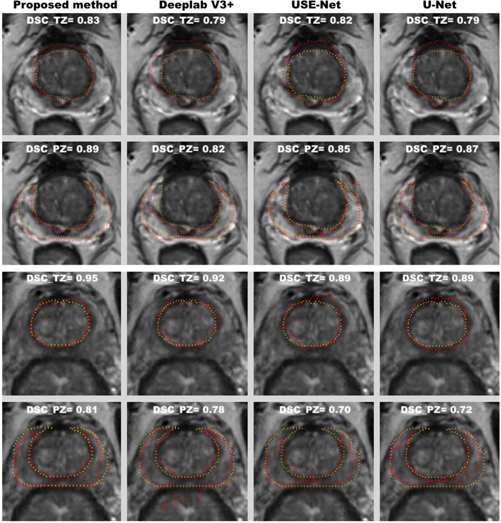
Two representative examples of the zonal segmentation by the proposed method, DeeplabV3₊ USE-Net, U-Net. Yellow lines are the manually annotated zonal segmentation, and the red lines are algorithmic results. The top two and bottom two rows represent the segmentation examples from two different subjects.

USE-Net was proposed by Rundo et al for the prostate zonal segmentation, which embeds the squeeze-and-excitation (SE) block into the U-Net and enables the adaptive channel-wise feature recalibration. Attention U-Net, proposed by Ozan et al, which incorporates attention gates into the standard U-Net architecture to highlight salient features that passes through the skip connections. Deeplab V3+ [23] is one of the state-of-art deep neural networks for image semantic segmentation, which takes the encoder-decoder architecture to recover the spatial information and utilizes multi-scale features by using atrous spatial pyramid pooling (ASPP). Convolutional features at multiple scales are probed by ASPP via applying several parallel atrous convolutions with different rates. R2U-Net is an extension of standard U-Net using recurrent neural network and residual neural networks.

Means and standard deviations of DSCs for PZ and TZ on ITD and ETD are shown in Table II. Mean DSCs for PZ and TZ of the proposed method were 0.80 and 0.89 on ITD, 0.79 and 0.87 on ETD, which were all higher than the results obtained by the comparison methods with significant difference.

TABLE II.

Performance (DSC) of the proposed method and baselines on internal testing dataset (ITD) and external testing dataset (ETD). P values are the comparisons between the proposed methods and baselines in ITD and ETD.

Datasets	ITD		ETD
	PZ	TZ	PZ	TZ
Proposed Method	0.80±0.05	0.89±0.04	0.79±0.06	0.87±0.07
Deeplab V3+	0.74±0.06 P<0.05	0.87±0.05 P<0.05	0.71±0.09 P<0.05	0.82±0.06 P<0.05
Attention U-Net	0.75±0.08 P<0.05	0.87±0.04 P<0.05	0.75±0.07 P<0.05	0.82±0.08 P<0.05
R2U-Net	0.70±0.10 P<0.05	0.85±0.05 P<0.05	0.69±0.08 P<0.05	0.78±0.10 P<0.05
USE-Net	0.72±0.10 P<0.05	0.86±0.06 P<0.05	0.72±0.08 P<0.05	0.80±0.08 P<0.05
U-Net	0.71±0.09 P<0.05	0.85±0.06 P<0.05	0.72±0.07 P<0.05	0.81±0.06 P<0.05

Means and standard deviations of Hausdorff Distance (HD) are shown in Table III. The proposed method achieved the lowest mean HD among all the methods for both PZ and TZ segmentation.

TABLE III.

Average Hausdorff Distance (mm) of the proposed method and baselines on internal testing dataset (ITD) and external testing dataset (ETD). P values are the comparisons between the proposed methods and baselines in ITD and ETD.

Datasets	ITD		ETD
	PZ	TZ	PZ	TZ
Proposed Method	4.77±2.86	3.52±1.81	5.96±3.13	4.92±2.73
Deeplab V3+	5.48±2.55 P=0.26	5.33±4.50 P<0.05	7.72±4.47 P<0.05	7.45±5.36 P<0.05
Attention	5.79±3.96	5.27±4.28	7.60±4.82	5.92±4.02
U-Net	P=0.14	P<0.05	P=0.06	P=0.13
R2U-Net	5.46±2.76 P=0.23	6.24±4.76 P<0.05	7.89±4.64 P<0.05	10.01±8.54 P<0.05
USE-Net	8.61±6.83 P<0.05	7.90±6.27 P<0.05	9.74±7.06 P<0.05	10.96±9.03 P<0.05
U-Net	8.88±7.63 P<0.05	11.38±7.63 P<0.05	9.72±6.06 P<0.05	11.55±6.54 P<0.05

Figure 4 showed the superior and inferior cases for the PZ and TZ segmentation. The superior case had DSC > 0.90 for PZ segmentation and DSC > 0.95 for TZ segmentation. DSCs of the inferior case were lower than 0.60 and 0.50 for the PZ and TZ segmentations, respectively.

Fig. 4.

Superior and inferior cases for PZ and TZ segmentation. Superior and inferior cases for PZ and TZ are shown in the first and second row.

B. PERFORMANCE DISCREPANCY BETWEEN THE INTERNAL TESTING DATASET (ITD) AND EXTERNAL TESTING DATASET (ETD)

There was no significant difference (p<0.05) between ITD and ETD for the performance of PZ segmentation for the proposed method. However, there was a 2.2% difference for the TZ segmentation (Table II).

C. PERFORMANCE INVESTIGATION FOR EACH INDIVIDUAL MODULE IN THE PROPOSED METHOD

We carried out the following ablation studies to investigate the importance of each module within the proposed network. TABLE IV indicates which module was used (a checkmark) or not used (a cross) in each experiment. We showed that the best model performance is achieved when both SAM and MFPA are used in the model for the zonal segmentation.

TABLE IV.

Performance investigation for each individual module of the proposed method. Average DSCs with standard deviation are shown in the table. SAM is the spatial attention module. MFPA is the multi-scale feature pyramid attention. Apart from the proposed method, there are two additional independent experiments, where √ and × under each row indicates whether the experiment contains the module or not.

			ITD		ETD
Experiments	SAM	MFPA	PZ	TZ	PZ	TZ
Proposed method	√	√	0.80±0.05	0.89±0.04	0.79±0.06	0.87±0.07
Experiment 1	×	√	0.79±0.07	0.88±0.04	0.77±0.07	0.85±0.07
Experiment 2	√	×	0.78±0.07	0.88±0.04	0.77±0.06	0.85±0.07

In experiment 1, DSCs for both zones on ITD and ETD decreased and were lower than the proposed model when SAM was removed from the proposed model, which proved that SAM helped improve the overall segmentation performance. In experiment 2, DSCs for PZ on ITD, and both zones on ETD decreased when MFPA was removed from the proposed model, indicating that that GFM was essential within the model.

D. THE OVERALL UNCERTAINTY FOR THE PROSTATE ZONAL SEGMENTATION OF THE PROPOSED METHOD

Figure 5 and TABLE V shows the overall uncertainties of the proposed method for the prostate zonal segmentation. The pixel-by-pixel uncertainty maps showed that the zonal boundaries had higher uncertainties than the interior areas at the three prostate locations (apex, middle, and base slices). Also, highest uncertainties were observed at the intersection between the PZ, TZ and the AFS.

Fig. 5.

The pixel-by-pixel uncertainty estimation of the zonal segmentation at the apex, middle, and base slices of the prostate (top). The orange color indicates high uncertainties, and blue color indicates low uncertainties. Bottom: Average uncertainty scores (bottom left) and average normalized DSCs (bottom right; normalized by TZ DSC − 0.87 shown in in Table IV) with the standard deviation at the apex, middle, and base slices of the prostate (x-axis).

TABLE V.

First two rows: Average uncertainty scores for all prostate, apex, middle, and base slices in PZ and TZ. Last two rows: DSCs for all prostate, apex, middle and base slices in PZ and TZ.

	All	Apex	Middle	Base
PZ Uncertainty	0.16±0.02	0.14±0.03	0.15±0.04	0.21±0.06
TZ Uncertainty	0.13±0.05	0.22±0.08	0.13±0.06	0.10±0.05
PZ DSC	0.79±0.06	0.81±0.10	0.82±0.08	0.63±0.28
TZ DSC	0.87±0.07	0.48±0.39	0.89±0.09	0.89±0.05

The TZ segmentation had lower overall uncertainties than the PZ segmentation, and the proposed method achieved better segmentation in TZ (DSC=0.87) compared to PZ (0.79). We used a normalized DSC (DSC_norm, normalized by TZ DSC – 0.87) to show relative differences at different locations of the prostate. For PZ segmentation, the highest overall uncertainty was observed at base, consistent with the worst model performance at base (DSC_norm 72.4%). For TZ segmentation, the highest overall uncertainty was observed at the apex, matched with the worst segmentation performance of the model at apex (DSC_norm 55.2%). Figure 5 bottom-left shows the average uncertainty estimation at different prostate locations, and the trend is well matched with the actual model performance (Fig. 5 bottom-right).

V. DISCUSSION

In this study, we proposed an attentive Bayesian deep learning model that accounts for long-range spatial dependencies between TZ and PZ with an estimation of pixel-wise uncertainties of the model. The performance discrepancy between ITD and ETD of the proposed model was minimal. There was no difference in PZ segmentation between ITD and ETD, and a 2.2% discrepancy in TZ segmentation. The average uncertainty estimation showed lower overall uncertainties for TZ segmentation than PZ, consistent with the actual segmentation performance difference between TZ and PZ. We attribute this to the complicated and curved shapes of PZ. The PZ boundaries generally have bilateral crescentic shapes, while the TZ boundaries are ellipsoid in shape.

SAM aided the model to focus on certain spatial areas in the zonal segmentation. This was done by the modeling of spatial dependencies with the help of global features. Since spatial attention was inserted adjacent to the raw images, large GPU memory was required to obtain the global spatial features during the training and evaluation. The SAM can be inserted into other positions within the network, but we observed that the zonal segmentation performed the best when the SAM followed directly after the raw image.

There exist high segmentation uncertainties on the zonal boundaries. This may be explained by the inconsistent manual annotations since the boundaries between TZ and PZ are hard to be defined precisely due to partial volume artifact. This resembles the “random error”, which persists throughout the entire experiment, so we call such uncertainty “random uncertainty” in the prostate zone segmentation.

The areas with the highest uncertainty are located at the junction of AFS, PZ and TZ. One possible reason is that it is hard for the MRI to distinguish the tissue around the junction. There is probably a significant reduction of signal by the more severe partial volume artifacts caused by PZ with the high pixel intensity, TZ with the intermediate pixel intensity and AFS with lower pixel intensity.

The overall uncertainties were higher at apex slices than those at base slices for the TZ segmentation. This may be caused by the fact that the size of TZ gradually increases from apex to base slices, making it hard to recognize the zone for the model. In contrast, the overall uncertainties for PZ were higher at the base slices than at the apex and middle slices. Similar to TZ, we attributed the low uncertainties to the large PZ structure between apex and middle slices [27] (Figure 6).

Fig. 6.

Prostate zonal anatomy at apex, middle, and base slices of the prostate.

The estimation of pixel-wise uncertainties of the prostate zonal segmentation would provide confidence and trust in an automatic segmentation workflow, which allows a simple rejection or acceptance based on a certain uncertainty level. This can be implemented as a partial or entire rejection of the automatic segmentation results when presenting to experts, and future research will be needed to determine the level of uncertainties to be acceptable to experts. We believe that this additional confidence would enable more natural adaption or acceptance of the automatic prostate segmentation than the one without it when the prostate segmentation is integrated into the downstream analysis decision.

We observed that simple incorporation of the inter-slice information by 3D U-Net was not sufficient to improve the segmentation performance. Our prostate MRI data had a lower through-plane resolution (3–3.6 mm) than the in-plane resolution (0.5–0.65 mm), resulting in a conflict between the anisotropism of the 3D images and isotropism of the 3D convolutions [28], [29]. This may be the main reason that the model’s generalization was compromised. Specifically, voxels in the x-z plane will correspond to the structure with different scales along x- and z-axes after the 3D convolution [27]. Moreover, the performance was more significantly different when both ITD and ETD were used for testing, potentially due to the difference in the imaging protocol. Further study may be needed to investigate advanced approaches that incorporate the inter-slice information into the 3D convolution when there exists a difference between in-plane and through-plane resolutions while minimizing sensitivities to different imaging protocols.

The significant effect of including SAM and MFPA was investigated in the ablation study. The average DSCs of the proposed method were higher than the experiments in the ablation study for PZ and TZ in both datasets. However, there were no significant differences between DSCs obtained by the experimental methods and the proposed method for both zones in the ablation study when a paired t-test was used. Based on the power analysis, we need 100, 253, 143, and 194 cases for Experiment 1 in Table IV (when SAM is removed) and 394, 253, 143, and 194 cases for Experiment 2 (when MFPA is removed) to achieve 80% power with alpha = 0.05.

We also compared the uncertainty of the proposed method and that of the U-Net. We found that average uncertainty scores of the proposed method for both PZ and TZ at three different prostate locations are all smaller than U-Net (Table VI).

TABLE VI.

Row 2 – 4: Average uncertainty scores for all prostate, apex, middle, and base slices in PZ and TZ under the proposed method. Row 5 – 7: Average uncertainty scores for all prostate, apex, middle, and base slices in PZ and TZ under U-Net.

Zone	All	Apex	Middle	Base
Proposed Method
PZ Uncertainty	0.16±0.02	0.14±0.03	0.15±0.04	0.21±0.06
TZ Uncertainty	0.13±0.05	0.22±0.08	0.13±0.06	0.10±0.05
U-Net
PZ Uncertainty	0.26±0.03	0.25±0.04	0.26±0.04	0.31±0.06
TZ Uncertainty	0.15±0.04	0.26±0.06	0.15±0.04	0.15±0.03

Our study still has a few limitations. First, the training time was long due to small batch sizes to extract the global features which also required a large GPU memory. Second, all MR images were acquired without the use of an endorectal coil in the study. This mirrors general clinical use since the use of endorectal coil is decreasing due to patients’ preference. Also, studies showed no significant difference for the detection of PCa between MR images acquired with and without the endorectal coil [28], [29] due to the increased signal-to-noise ratios (SNRs) and spatial resolution of 3T MRI scanners, compared to 1.5T. We can apply pixel-to-pixel translation techniques such as cycle-GAN to handle the cases with an endorectal coil since the images with the endorectal coil contain large signal variations near the coil. Third, the study considered the slices that contain the prostate, which could potentially reduce the false positives of the non-prostate slices and increase the overall segmentation performance.

VI. CONCLUSION

We proposed a spatial attentive Bayesian deep learning model for the automatic segmentation of prostatic zones with pixel-wise uncertainty estimation. The study showed that the proposed method is superior to the state-of-art methods (U-Net and USE-Net) on the segmentation of two prostate zones, such as TZ and PZ. Both spatial attention and multiple-scale feature pyramid attention modules had their merits for the prostate zonal segmentation. Also, the overall uncertainties by the Bayesian model demonstrated different uncertainties between TZ and PZ at three prostate locations (apex, middle and base), which was consistent with the actual model performance evaluated by using internal and external testing data sets.

Biography

YONGKAI LIU received his M.S. degree in biomedical engineering department from Tsinghua University, Beijing, China, in 2017. He is currently pursuing the Ph.D. in physics and biology in medicine program, David Geffen School of Medicine. He has two first-author journal papers concerning virtual colonoscopy and one demo presentation of ICCV (International Conference On Computer Vision) concerning medical image segmentation using deep learning. His current research interest is medical image processing using deep learning. The honors & awards he obtained were PhD Fellowship of UCLA PBM, partial funding support 2016 Gorden Research Conference (GRC) on Image Science, Champion in Youth Innovation and Entrepreneurship

GUANG YANG. (B.Eng, M.Sc., Ph.D., M.IEEE,.ISMRM, M.SPIE) obtained his M.Sc. in Vision Imaging and Virtual Environments from the Department of Computer Science in 2006 and his Ph.D. on medical image analysis jointly from the CMIC, Department of Computer Science and Medical Physics in 2012 both from University College London. He is currently an honorary lecturer with the Neuroscience Research Centre, Cardiovascular and Cell Sciences Institute, St. George’s, University of London. He is also an image processing physicist and honorary senior research fellow working at Cardiovascular Research Centre, Royal Brompton Hospital and also affiliate with National Heart and Lung Institute, Imperial College London.

QI MIAO is currently a research scholar at the abdominal radiology department of David Geffen School of Medicine at UCLA. She received her Medical Doctorate degree from China Medical University in 2013. She completed her residency training as a radiologist at the First Hospital of China Medical University in 2017. She started her research fellowship at Abdominal Imaging/Cross Sectional Interventional Radiology department at UCLA in 2020.

MELINA HOSSEINY, M.D. is a postdoctoral research fellow at the abdominal radiology department of David Geffen School of Medicine at UCLA under the supervision of Dr. Steven S. Raman. After entering med school, she completed her clinical rotations and internship at Tehran University of Medical Sciences (TUMS). She has been an active member of the UCLA Prostate IDx group at UCLA since 2018. She pioneered the creation of the ever-growing database for inbore MR-guided biopsy of the prostate at UCLA, which she has presented at several national radiology meetings. Her current research interests include in-bore MR guided biopsy of the prostate, improving the image quality of prostate MRI, and investigation of CT scan for prediction of renal tumors microenvironment with the creation of machine and deep learning models.

STEVEN S. RAMAN. received the M.D. degree from the Keck School of Medicine of USC, Los Angeles, in 1993. He is currently an Expert in abdominal and pelvic imaging (CT, MRI, US and X-Ray) and interventional radiology (image guided procedures), especially in the area of tumor ablation and fibroid treatment. He is also the Director of the Abdominal Imaging Fellowship at UCLA, and the Co-Director of the Fibroid Treatment Program at UCLA.

AFSHIN AZADIKHAH received the M.D. degree from the Iran University of Medical Sciences, Iran, in 2014. He started his research fellowship at the Abdominal Imaging/Cross Sectional Interventional Radiology Department, UCLA, in 2018. He is currently a Postdoctoral Research Scholar with the Radiology Department, UCLA.

SOHRAB AFSHARI MIRAK received the M.D. degree from the Tehran University of Medical sciences (TUMS), Tehran, Iran, in 2013. He started his research fellowship at the Abdominal Imaging/Cross Sectional Interventional Radiology Department, UCLA, in 2017. He is currently a Postdoctoral Research Scholar with the Radiology Department, UCLA. He is also a member of the Prostate MR Imaging and Interventions and UCLA Prostate MR Imaging Research Group.

KYUNGHYUN SUNG received the Ph.D. degree in electrical engineering from the University of Southern California, Los Angeles, in 2008. From 2008 to 2012, he finished his postdoctoral training with the Departments of Radiology, Stanford. In 2012, he joined the Department of Radiological Sciences, University of California at Los Angeles, Los Angeles (UCLA). He is currently an Associate Professor of Radiology, where his research primarily focuses on the development of novel medical imaging methods and artificial intelligence using magnetic resonance imaging (MRI). In particular, his research group (https://mrrl.ucla.edu/sunglab/) is currently focused on developing advanced deep learning algorithms and quantitative MRI techniques for early diagnosis, treatment guidance, and therapeutic response assessment for oncologic applications. Such developments can offer more robust and reproducible measures of biologic markers associated with human cancers.

REFERENCES

- [1].Ghafoori M, Alavi M, and Aliyari Ghasabeh M, “MRI in Prostate Cancer,” Iranian Red Crescent Medical Journal, vol. 15, no. 12, December 2013, doi: 10.5812/ircmj.16620. [DOI] [PMC free article] [PubMed] [Google Scholar]
- [2].Turkbey B. et al. , “Prostate Imaging Reporting and Data System Version 2.1: 2019 Update of Prostate Imaging Reporting and Data System Version 2,” European Urology, March 2019, doi: 10.1016/j.eururo.2019.02.033. [DOI] [PubMed] [Google Scholar]
- [3].Weinreb JC et al. , “PI-RADS prostate imaging–reporting and data system: 2015, version 2,” European urology, vol. 69, no. 1, pp. 16–40, 2016. [DOI] [PMC free article] [PubMed] [Google Scholar]
- [4].Sonn GA et al. , “Value of targeted prostate biopsy using magnetic resonance–ultrasound fusion in men with prior negative biopsy and elevated prostate-specific antigen,” European urology, vol. 65, no. 4, pp. 809–815, 2014. [DOI] [PMC free article] [PubMed] [Google Scholar]
- [5].Liu Y. et al. , “Automatic Prostate Zonal Segmentation Using Fully Convolutional Network With Feature Pyramid Attention,” IEEE Access, vol. 7, pp. 163626–163632, 2019. [Google Scholar]
- [6].Meyer A. et al. , “Towards Patient-Individual PI-Rads v2 Sector Map: Cnn for Automatic Segmentation of Prostatic Zones From T2-Weighted MRI,” in 2019 IEEE 16th International Symposium on Biomedical Imaging (ISBI 2019), 2019, pp. 696–700, doi: 10.1109/ISBI.2019.8759572. [DOI] [Google Scholar]
- [7].Hosseinzadeh M, Brand P, and Huisman H, “Effect of Adding Probabilistic Zonal Prior in Deep Learning-based Prostate Cancer Detection,” in International Conference on Medical Imaging with Deep Learning – Extended Abstract Track, 2019. [Google Scholar]
- [8].Padgett K, Swallen A, Nelson A, Pollack A, and Stoyanova R, “SU-F-J-171: Robust Atlas Based Segmentation of the Prostate and Peripheral Zone Regions On MRI Utilizing Multiple MRI System Vendors,” Medical physics, vol. 43, no. 6Part11, p. 3447, 2016. [Google Scholar]
- [9].Zabihollahy F, Schieda N, Krishna Jeyaraj S, and Ukwatta E, “Automated segmentation of prostate zonal anatomy on T2-weighted (T2W) and apparent diffusion coefficient (ADC) map MR images using U-Nets,” Medical physics, 2019. [DOI] [PubMed] [Google Scholar]
- [10].Clark T, Zhang J, Baig S, Wong A, Haider MA, and Khalvati F, “Fully automated segmentation of prostate whole gland and transition zone in diffusion-weighted MRI using convolutional neural networks,” Journal of Medical Imaging, vol. 4, no. 4, p. 41307, 2017. [DOI] [PMC free article] [PubMed] [Google Scholar]
- [11].He K, Zhang X, Ren S, and Sun J, “Deep residual learning for image recognition,” in Proceedings of the IEEE conference on computer vision and pattern recognition, 2016, pp. 770–778. [Google Scholar]
- [12].Rundo L. et al. , “USE-Net: Incorporating Squeeze-and-Excitation blocks into U-Net for prostate zonal segmentation of multi-institutional MRI datasets,” Neurocomputing, vol. 365, pp. 31–43, 2019. [Google Scholar]
- [13].Nair T, Precup D, Arnold DL, and Arbel T, “Exploring uncertainty measures in deep networks for multiple sclerosis lesion detection and segmentation,” Medical image analysis, vol. 59, p. 101557, 2020. [DOI] [PubMed] [Google Scholar]
- [14].Wang X, Girshick R, Gupta A, and He K, “Non-local neural networks,” in Proceedings of the IEEE Conference on Computer Vision and Pattern Recognition, 2018, pp. 7794–7803. [Google Scholar]
- [15].Gal Y. and Ghahramani Z, “Dropout as a bayesian approximation: Representing model uncertainty in deep learning,” in international conference on machine learning, 2016, pp. 1050–1059. [Google Scholar]
- [16].Litjens G, Debats O, Barentsz J, Karssemeijer N, and Huisman H, “Computer-aided detection of prostate cancer in MRI,” IEEE transactions on medical imaging, vol. 33, no. 5, pp. 1083–1092, 2014. [DOI] [PubMed] [Google Scholar]
- [17].Mukhoti J. and Gal Y, “Evaluating bayesian deep learning methods for semantic segmentation,” arXiv preprint arXiv:181112709, 2018. [Google Scholar]
- [18].Gal Y, “Uncertainty in deep learning,” University of Cambridge, vol. 1, p. 3, 2016. [Google Scholar]
- [19].Kendall A. and Gal Y, “What uncertainties do we need in bayesian deep learning for computer vision?,” in Advances in neural information processing systems, 2017, pp. 5574–5584. [Google Scholar]
- [20].Myronenko A. and Song X, “Point set registration: Coherent point drift,” IEEE transactions on pattern analysis and machine intelligence, vol. 32, no. 12, pp. 2262–2275, 2010. [DOI] [PubMed] [Google Scholar]
- [21].Chen L-C, Papandreou G, Kokkinos I, Murphy K, and Yuille AL, “Deeplab: Semantic image segmentation with deep convolutional nets, atrous convolution, and fully connected crfs,” IEEE transactions on pattern analysis and machine intelligence, vol. 40, no. 4, pp. 834–848, 2017. [DOI] [PubMed] [Google Scholar]
- [22].Chen L-C, Papandreou G, Kokkinos I, Murphy K, and Yuille AL, “Deeplab: Semantic image segmentation with deep convolutional nets, atrous convolution, and fully connected crfs,” IEEE transactions on pattern analysis and machine intelligence, vol. 40, no. 4, pp. 834–848, 2017. [DOI] [PubMed] [Google Scholar]
- [23].Chen LC, Zhu Y, Papandreou G, Schroff F, and Adam H, “Encoder-decoder with atrous separable convolution for semantic image segmentation,” in Lecture Notes in Computer Science (including subseries Lecture Notes in Artificial Intelligence and Lecture Notes in Bioinformatics), 2018, vol. 11211 LNCS, pp. 833–851, doi: 10.1007/978-3-030-01234-2_49. [DOI] [Google Scholar]
- [24].Ronneberger O, Fischer P, and Brox T, “U-net: Convolutional networks for biomedical image segmentation,” in International Conference on Medical image computing and computer-assisted intervention, 2015, pp. 234–241. [Google Scholar]
- [25].Oktay O. et al. , “Attention u-net: Learning where to look for the pancreas,” arXiv preprint arXiv:1804.03999, 2018. [Google Scholar]
- [26].Alom MZ, Hasan M, Yakopcic C, Taha TM, and Asari VK, “Recurrent residual convolutional neural network based on u-net (r2u-net) for medical image segmentation,” arXiv preprint arXiv:1802.06955, 2018. [Google Scholar]
- [27].Chen J, Yang L, Zhang Y, Alber M, and Chen DZ, “Combining fully convolutional and recurrent neural networks for 3d biomedical image segmentation,” in Advances in neural information processing systems, 2016, pp. 3036–3044. [Google Scholar]
- [28].Barth BK et al. , “Diagnostic Accuracy of a MR Protocol Acquired with and without Endorectal Coil for Detection of Prostate Cancer: A Multicenter Study,” Current urology, vol. 12, no. 2, pp. 88–96, 2018. [DOI] [PMC free article] [PubMed] [Google Scholar]
- [29].Mirak SA et al. , “Three Tesla Multiparametric Magnetic Resonance Imaging: Comparison of Performance with and without Endorectal Coil for Prostate Cancer Detection, PI-RADSTM version 2 Category and Staging with Whole Mount Histopathology Correlation,” The Journal of urology, vol. 201, no. 3, pp. 496–502, 2019. [DOI] [PubMed] [Google Scholar]