Low frequency conductivity reconstruction based on a single current injection via MREIT

Abstract

Conventional MREIT reconstruction methods require administration of two linearly independent currents via at least two electrode pairs. This requires long scanning times and inhibits coordination of MREIT measurements with electrical neuromodulation strategies. We sought to develop an isotropic conductivity reconstruction algorithm in MREIT based on a single current injection, both to decrease scanning time by a factor of two and enable MREIT measurements to be conveniently adapted to general transcranial- or implanted-electrode neurostimulation protocols. In this work, we propose and demonstrate an iterative algorithm that extends previously published MREIT work using two-current administration approaches. The proposed algorithm is a single-current adaptation of the harmonic B_z algorithm. Forward modeling of electric potentials is used to capture changes of conductivity along current directions that would normally be invisible using data from a single-current administration. Computational and experimental results show that the reconstruction algorithm is capable of reconstructing isotropic conductivity images that agree well in terms of L² error and structural similarity with exact conductivity distributions or two-current-based MREIT reconstructions. We conclude that it is possible to reconstruct high quality electrical conductivity images using MREIT techniques and one current injection only.

1. Introduction

Low-frequency conductivity properties of biological tissue are related to the concentration and mobility of ions and other charge carriers in the extracellular fluid, as well as cell concentration and geometry (Grimnes and Martinsen 2015). These quantities vary markedly in different disease states. Magnetic resonance electrical impedance tomography (MREIT) provides a method of producing high-resolution, low-frequency electrical conductivity images. MREIT has been used to evaluate conductivity contrasts in disease models such as brain abscess and cerebral ischemia (Oh et al. 2013, Kim et al. 2015) or tumor detection (Muftuler et al. 2004). Recently, MREIT methods have also been proposed for monitoring therapeutic electromagnetic field distributions in electroporation (Kranjc et al. 2011, Kranjc et al. 2015), transcranial direct current stimulation (tDCS) (Kasinadhuni et al. 2017, Kwon et al. 2016) and deep brain stimulation (DBS) (Sajib et al. 2017a).

In a typical MREIT experiment, an object is placed inside the MRI bore with pairs of surface electrodes attached. A low frequency current is administered via these electrodes, which creates a voltage distribution u, current density J = (J_x, J_y, J_z) and magnetic flux density B = (B_x, B_y, B_z) distribution inside the object. Only the component of the magnetic flux density parallel to the main magnetic field axis (z), B_z, can be measured in MRI phase images (Woo and Seo 2008). Measured B_z data can be used to reconstruct the conductivity distribution via the Biot-Savart law (Stratton 1941).

In order to measure all three components of B, it is necessary to rotate the object inside the MRI scanner (Joy et al. 1989). Current density images may then be obtained directly via Ampere’s law (Scott et al. 1992). However, object rotation is often impractical and may cause registration or conformation errors (Khang et al. 2002). Further, (Kwon et al. 2002) proposed the J-substitution algorithm, which uses fully measured B = (B_x, B_y, B_z) vectors to reconstruct conductivity distributions. While the method can be used to reconstruct the absolute conductivity distribution of a conductive phantom (Khang et al. 2002), as in (Scott et al. 1992) it requires acquisition of the full B vector field, and it is thus not possible to apply this method to animal or human subject data.

Meanwhile, it has been demonstrated that it is possible to reconstruct high-resolution electrical conductivity from B_z alone (Woo and Seo 2008, Seo and Woo 2011, Seo and Woo 2014), and algorithms based on this show promise for clinical MREIT applications (Kim et al. 2007, Kim et al. 2009). Examples of such algorithms are the harmonic (Oh et al. 2003, Seo et al. 2003) and non-iterative (Seo et al. 2011) harmonic B_z algorithms; the gradient B_z decomposition algorithm (Park et al. 2004a); variational gradient B_z algorithm (Park et al. 2004b); as well as algorithms based on current densities estimated from B_z (Gao and He 2008, Nam et al. 2008, Oran and Ider 2012, Sajib et al. 2012, Jeon et al. 2017) and the recently proposed reduced basis approach (Garmatter and Harrach 2018). However, all these algorithms require administration of two linearly independent currents to produce conductivity images.

There are several technical issues which need to be carefully considered in developing practical clinical applications of MREIT, with a key issue being the need to improve acquisition efficiency while maintaining data quality. One approach to accelerate MREIT data acquisition is to skip phase encoding steps and reconstruct B_z images from undersampled data (Song et al. 2016, Song et al. 2017, Song et al. 2018). Since use of high MREIT imaging currents may produce undesirable nerve stimulation effects (Seo and Woo 2014, Sadleir et al. 2019) another consideration is acquiring high signal-to-noise ratio (SNR) B_z data without using larger electric currents. The transversal J-substitution algorithm was proposed by (Nam et al. 2007) for use with low amplitude current. However, since the method requires computation of gradients of B_z data, effects of stray magnetic fields due to currents in wires and electrodes must be calculated and corrected (Lee et al. 2003, Nam et al. 2007).

In transcranial electrical stimulation, montages do not generally involve administration of multiple linearly independent currents, and most often use only one pair of large electrodes located over target brain structures (Bikson et al. 2019). Typical tDCS protocols involve alternating or direct current applied with amplitudes of up to 4 mA (Nitsche and Bikson 2017). The use of neuromodulation therapies also provides a unique opportunity to image conductivity distributions, which may be of use in constructing subject-specific computational models used for treatment planning, whereas conventional models have used conductivities for brain tissues derived from literature values (Sadleir et al. 2010).

Without prior knowledge informing conductivity reconstructions, the single-current MREIT reconstruction problem is in general ill-posed (Kim et al. 2003). If we assume that a single current injection produces a current density J inside the imaged object, all possible solutions can be decomposed into a desired solution and artifacts, where artifacts depend heavily on the current density generated by the imaging current. Indeed, these artifacts do not change along the direction orthogonal to current flow directions. Fortunately, the features of these artifacts are relatively simple, due to their close association with J, and therefore it is not difficult to find a suitable image prior to remove them. For example, knowledge of the object boundary conductivity can eliminate these artifacts. Deep learning techniques can be used to remove artifacts when sufficient training data is available (Mandija et al. 2019, Seo et al. 2019, Sajib et al. 2020).

Single-current MREIT conductivity imaging approaches have been proposed previously. For example (Lee et al. 2010) estimated projected current density (Park et al. 2007a) from one set of B_z data and applied Kirchhoff’s voltage law (KVL) to a mimetic discretized network to demonstrate that it is possible to reconstruct conductivity images using a single current administration. Unfortunately, the quality of the reconstructed conductivity images is not acceptable for clinical use because of noise propagation perpendicular to the current flow direction (Lee et al. 2010). Other methods have involved minimizing artifacts by applying regularization (Oran and Ider 2012), however, this approach may lead to oversmoothing.

In this paper, we propose a new isotropic conductivity reconstruction algorithm based on a single current administration, the single-current harmonic B_z algorithm. To avoid two current administrations, we take advantage of the divergence-free condition of the current density ∇ · J = 0 to iteratively update the internal conductivity distribution σ. It is demonstrated that the proposed algorithm is stable against noise and numerical errors in both numerical simulations and phantom experiments.

2. Reconstruction methods

2.1. Preliminaries

Let the object to be imaged constitute a three dimensional domain $\Omega \subset {\mathbb{R}}^3$ with a smooth boundary ∂Ω. We denote the positive isotropic conductivity distribution at any point r = (x, y, z) within Ω as σ(r). In MREIT, an external current with amplitude I is injected between a pair of surface electrodes Ɛ^±, (see Figure 1(a)) producing a voltage distribution, u(r), such that

$$\{\begin{array}{c}-\nabla \cdot (\sigma \nabla u)=0\text{in}\Omega \hfill \\ {\int }_{{\mathcal{E}}^{+}}\sigma \frac{\partial u}{\partial \mathbf{n}}dS=I=-{\int }_{{\mathcal{E}}^{-}}\sigma \frac{\partial u}{\partial \mathbf{n}}dS\hfill \\ \nabla u\times \mathbf{n}{\mid }_{{\mathcal{E}}^{\pm }}=0\hfill \\ {\phantom{\mid }\sigma \frac{\partial u}{\partial \mathbf{n}}\mid }_{\partial \Omega \setminus \overline{{\mathcal{E}}^{+}\cup {\mathcal{E}}^{-}}}=0\hfill \\ {\int }_{\partial \Omega }udS=0.\hfill \end{array}\phantom{\}}$$ (1)

Figure 1.

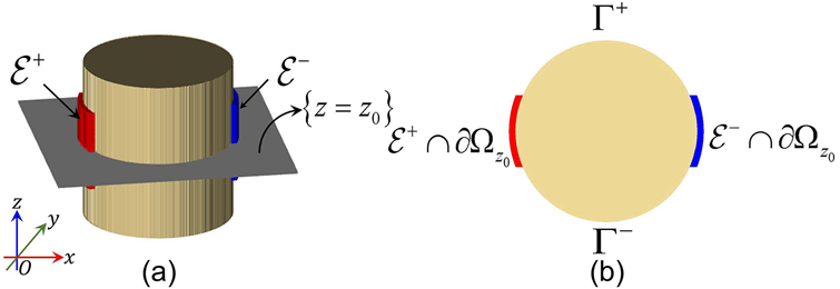
Illustration of three-dimensional cylindrical object with ‘horizontal’ surface electrodes Ɛ^± on the boundary of Ω. (a) Oblique view of object showing electrodes and central slice at z = z₀. (b) Central slice Ω_z0 with boundary notations Ɛ^± ∩ ∂Ω_z0 and Γ^±.

Here, n denotes the unit outward normal vector on ∂Ω, and dS denotes the surface area element.

The current density J = (J_x, J_y, J_z) in Ω associated with the solution of (1) is determined from Ohm’s law,

$$\mathbf{J}(\mathbf{r})=-\sigma (\mathbf{r})\nabla u(\mathbf{r}).$$ (2)

Further, the relation between the z-component of the magnetic flux density, B_z and the conductivity σ is described by the Biot-Savart law (Stratton 1941),

$$B_z(\mathbf{r})=\frac{{\mu }_0}{4\pi }{\int }_{\Omega }\frac{\langle \mathbf{r}-{\mathbf{r}}^{\prime },-\sigma \nabla u({\mathbf{r}}^{\prime })\times \widehat{\mathbf{z}}\rangle }{\mid \mathbf{r}-{\mathbf{r}}^{\prime }{\mid }^3}d{\mathbf{r}}^{\prime }\text{for}\mathbf{r}\in \Omega ,$$ (3)

where $\widehat{\mathbf{z}}=(0,0,1)$, μ₀ = 4π × 10⁻⁷ H/m is the magnetic permeability of free space, ⟨·, ·⟩ denotes the Euclidean inner product in ${\mathbb{R}}^3$ and ∣r – r′∣ denotes the Euclidean distance between r and r′ in Ω.

2.2. Current density reconstruction from B_z

The relationship between the current density J(r) = (J_x, J_y, J_z) and its associated magnetic flux density B(r) = (B_x, B_y, B_z) is described by Ampere’s law

$$\mathbf{J}(\mathbf{r})=\frac{1}{{\mu }_0}\nabla \times \mathbf{B}(\mathbf{r}).$$ (4)

If only one component of the current-induced magnetic flux density is measured in each image slice Ω_z0 ≔ Ω ∩ {z = z₀}, we may choose to reconstruct the current density information ${\mathbf{J}}^c=(J_x^c,J_y^c)$ using B_z alone, as in (Seo et al. 2011), where

$${\mathbf{J}}^c(\mathbf{r})=(J_x^c,J_y^c)={\nabla }_{\text{xy}}^{\perp }(\varphi +\beta \psi ).$$ (5)

Here, ${\nabla }_{\text{xy}}^{\perp }≔\left(\frac{\partial }{\partial y},-\frac{\partial }{\partial x}\right)$, and the terms ϕ and ψ in equation (5) are the solution of the following boundary value problems

$$\{\begin{array}{cc}{\nabla }_{\text{xy}}^2\varphi =\frac{1}{{\mu }_0}{\nabla }^2{B}_z\hfill & \text{in}{\Omega }_{z_0}\hfill \\ \nu \cdot {\nabla }_{\text{xy}}\varphi =0\hfill & \text{on}({\mathcal{E}}^{+}\cup {\mathcal{E}}^{-})\cap {\Omega }_{z_0}\hfill \\ \varphi =0\hfill & \text{on}{\Gamma }^{+}\cup {\Gamma }^{-}\hfill \end{array}\phantom{\}}$$ (6)

and

$$\{\begin{array}{cc}{\nabla }_{\text{xy}}^2\psi =0\hfill & \text{in}{\Omega }_{z_0}\hfill \\ \nu \cdot {\nabla }_{\text{xy}}\psi =0\hfill & \text{on}({\mathcal{E}}^{+}\cup {\mathcal{E}}^{-})\cap {\Omega }_{z_0}\hfill \\ \psi {\mid }_{{\Gamma }^{\pm }}=\pm 1,\hfill & \hfill \end{array}\phantom{\}}$$ (7)

where ${\nabla }_{\text{xy}}=(\frac{\partial }{\partial x},\frac{\partial }{\partial y})$ is the transverse gradient operator, Γ^± ⊂ ∂Ω_z0 satisfying that Ɛ⁺ ∩ ∂Ω_z0, Γ⁺, Γ⁻ and Ɛ⁻ ∩ ∂Ω_z0 are in the direction of counterclockwise (See Figure 1 (b)). The scaling factor β is defined as

$$\beta =\frac{{\int }_{{\mathcal{E}}^{+}\cap \partial {\Omega }_{z_0}}\sigma {\nabla }_{\text{xy}}u\cdot \nu d\ell -{\int }_{{\mathcal{E}}^{+}\cap \partial {\Omega }_{z_0}}{\nabla }_{\text{xy}}\varphi \times \nu d\ell }{{\int }_{{\mathcal{E}}^{+}\cap \partial {\Omega }_{z_0}}{\nabla }_{\text{xy}}\psi \times \nu d\ell }$$ (8)

where dℓ is the arc length element and ν is the two-dimensional unit outward normal vector to ∂Ω_z0.

For the derivation of formula (8), refer to Observation 4.1 and its proof in (Seo et al. 2011).

2.3. Proposed single-current harmonic B_z reconstruction method

In this section we describe the proposed single-current conductivity reconstruction algorithm. Applying the curl operator on both sides of (4), we obtain

$${\nabla }_{\text{xy}}^{\perp }u\cdot {\nabla }_{\text{xy}}\sigma =\frac{1}{{\mu }_0}{\nabla }^2{B}_z.$$ (9)

From (2) and (9) and normalizing conductivity to 1 S/m we obtain

$$(J_y,-J_x)\cdot {\nabla }_{\text{xy}}\text{ln}\sigma =-\frac{1}{{\mu }_0}{\nabla }^2{B}_z.$$ (10)

Next, using the divergence-free condition of the current density ∇·J = ∇·(−σ∇u) = 0 we obtain,

$${\nabla }_{\text{xy}}u\cdot {\nabla }_{\text{xy}}\sigma =-\sigma {\nabla }^{2}u-\frac{\partial u}{\partial z}\frac{\partial \sigma }{\partial z}.$$ (11)

Since we assume an isotropic conductivity distribution, Ohm’s law (2) allows substitution of ∇_xyu with $-\frac{1}{\sigma }(J_x,J_y)$ in (11) to obtain

$$(J_x,J_y)\cdot {\nabla }_{\text{xy}}\text{ln}\sigma =\sigma {\nabla }^{2}u+\frac{\partial u}{\partial z}\frac{\partial \sigma }{\partial z}.$$ (12)

For the current pattern defined in (1), the current density ∣J∣ ≠ 0 in Ω_z0 (Kim et al. 2002, Nachman et al. 2009). Therefore, we can recover ∇_xy ln σ by solving the system formed by (10) and (12).

This leads to the following expression for ∇_xy ln σ

$${\nabla }_{\text{xy}}\text{ln}\sigma =\mathrm{s}\text{in}{\Omega }_{z_0},$$ (13)

where s is the vector defined as

$$\mathrm{s}=\frac{1}{J_x^2+J_y^2}\left[\begin{array}{c}\hfill \sigma J_x({\nabla }^{2}u+\frac{\partial u}{\partial z}\frac{\partial \text{ln}\sigma }{\partial z})-\frac{1}{{\mu }_0}{J}_y{\nabla }^2{B}_z\hfill \\ \hfill \sigma J_y({\nabla }^{2}u+\frac{\partial u}{\partial z}\frac{\partial \text{ln}\sigma }{\partial z})+\frac{1}{{\mu }_0}{J}_x{\nabla }^2{B}_z\hfill \end{array}\right].$$

We propose an iterative equation to update the ∇_xy ln σ based on the identity in (13), using the estimated current density, J^c in equation (5). The n-th update for the imaging plane Ω_z0 may be written as

$${\nabla }_{\text{xy}}\text{ln}{\sigma }^{n+1}={\mathrm{s}}^{n+1},\text{for}n=0,1,2,\cdots ,$$ (14)

where

$${\mathrm{s}}^{n+1}=\frac{1}{J_x^{c^2}+J_y^{c^2}}\left[\begin{array}{c}\hfill {\sigma }^n{J}_x^c({\nabla }^2{u}^n+\frac{\partial u^n}{\partial z}\frac{\partial \text{ln}{\sigma }^n}{\partial z})-\frac{1}{{\mu }_0}{J}_y^c{\nabla }^2{B}_z\hfill \\ \hfill {\sigma }^n{J}_y^c({\nabla }^2{u}^n+\frac{\partial u^n}{\partial z}\frac{\partial \text{ln}{\sigma }^n}{\partial z})+\frac{1}{{\mu }_0}{J}_x^c{\nabla }^2{B}_z\hfill \end{array}\right].$$ (15)

To obtain ln σⁿ⁺¹ from ∇_xy ln σⁿ⁺¹ = sⁿ⁺¹, the following Poisson equation is solved

$$\{\begin{array}{cc}{\nabla }_{\text{xy}}^2\text{ln}{\sigma }^{n+1}={\nabla }_{\text{xy}}\cdot {\mathrm{s}}^{n+1}\hfill & \text{in}{\Omega }_{z_0}\hfill \\ \text{ln}{\sigma }^{n+1}=\text{ln}{\sigma }_b\hfill & \text{on}\partial {\Omega }_{z_0},\hfill \end{array}\phantom{\}}$$ (16)

where σ_b, is the boundary conductivity value.

We summarize the proposed single-current harmonic B_z method in Algorithm 1 below.

Algorithm 1 Single-current harmonic Bz algorithm

$$\begin{array}{cc}\hfill & \mathbf{Step}1.\text{Construct a numerical model for the nominated image slice}.\hfill \\ \hfill & \mathbf{Step}2.\text{Using equation}(6),\text{obtain}\varphi \text{from the}{B}_z\text{data}.\hfill \\ \hfill & \mathbf{Step}3.\text{Solve equation}(7)\text{for}\psi .\hfill \\ \hfill & \mathbf{Step}4.\text{Compute}{\mathbf{J}}^c\text{in}(5).\hfill \\ \hfill & \mathbf{Step}5.\text{Initialization: Specify a tolerance}{ϵ}_0\text{and maximum iteration number}N.\text{Set}\hfill \\ \hfill & n=0,ϵ={ϵ}_0,\text{and homogeneous initial guess}{\sigma }^0={\sigma }_b.\hfill \\ \hfill & \mathbf{while}(ϵ\ge {ϵ}_0\text{and}n<N)\mathbf{do}\hfill \\ \hfill & (\mathrm{i})\text{Solve equation}(1)\text{to obtain}{u}^n.\hfill \\ \hfill & (\mathrm{ii})\text{Using}{\mathbf{J}}^c\text{and}{u}^n,\text{compute the right hand side of equation (14)}.\hfill \\ \hfill & (\mathrm{iii})\text{Obtain an updated}{\sigma }^{n+1}\text{using equation (16)}\hfill \\ \hfill & (\mathrm{iv})\text{Compute the erroe}ϵ=\frac{\Vert {\sigma }^{n+1}-{\sigma }^n{\Vert }_{L^2({\Omega }_{z_0})}}{\Vert {\sigma }^n{\Vert }_{L^2({\Omega }_{z_0})}}.\hfill \\ \hfill & (\mathrm{v})\text{Set}n\leftarrow n+1.\hfill \\ \hfill & \mathbf{end}\mathbf{while}\hfill \\ \hfill & \mathbf{Step}6.\mathbf{return}{\sigma }^n.\hfill \end{array}$$

Remark 2.1. Assume $\mid \frac{\partial \text{ln}\sigma }{\partial z}\mid \ll 1$. If we use a long electrode and aim to reconstruct the conductivity distribution in the center slice, the current in the transversal plane will be dominant. Hence, the term $\frac{\partial u^n}{\partial z}\frac{\partial \text{ln}{\sigma }^n}{\partial z}\approx 0$. In this situation, the first update of (15) for ∇_xy ln σ¹ takes the following form

$${\mathrm{s}}^1=-\frac{1}{{\mu }_0}\frac{{\mathbf{J}}^{c^{\perp }}}{J_x^{c^2}+J_y^{c^2}}{\nabla }^2{B}_z,$$ (17)

where ${\mathbf{J}}^{c^{\perp }}≔(J_y^c,-J_x^c)$.

In the Appendix, we provide an error estimation for a single iteration reconstruction for a simple 2D case. In the Results section, we demonstrate that even a single iteration as in (17) produces high quality results in the sense of L² when the conductivity satisfies ∥∇ ln σ∥_L²(Ω) ≪ 1.

3. Numerical and tissue phantom tests

3.1. Numerical simulation set-up

To investigate the performance of the proposed single-current harmonic B_z algorithm, we simulated a three-dimensional cylindrical phantom model having a 45 mm diameter and 40 mm height using COMSOL (COMSOL, Burlingham MA, USA). Anomalies based on the modified Shepp-Logan phantom (Shepp and Logan 1974) were placed inside the cylinder. A pair of surface electrodes with dimension 5 × 10 mm² were attached to simulate current administration. Fig. 2(a) shows the phantom geometry and electrodes. The anomaly distribution within the center slice of the modified Shepp-Logan phantom is displayed in Fig. 2(b).

Figure 2.

Numerical simulation set-up. (a) Three-dimensional model of modified Shepp-Logan phantom defined using COMSOL (COMSOL, Burlingham MA, USA). (b) Anomaly distribution within the modified Shepp-Logan phantom for center imaging slice. For numerical Model A the conductivity values were set to 0.8, 1.0 and 1.2 S/m for low, background and the high contrast regions, respectively. Conductivity values for numerical Model B were 0.5, 1.0 and 2.0 S/m for low, background and the high contrast regions, respectively. (c) Simulated B_z images obtained using the Biot-Savart law (3) for ‘horizontal’ current injection. Parts (i) and (ii) show results for numerical Models A and B, respectively.

It is shown in the Appendix that the reconstruction error caused by one step of the single-current harmonic B_z algorithm is related to ∥∇ ln σ∥. To confirm this, we tested the method using both low and high-contrast conductivity distributions. In the low-contrast numerical Model A, conductivities of ellipsoidal regions were 0.8 S/m and conductivities in disk-shaped regions were 1.2 S/m (Fig. 2). In numerical Model B, anomaly conductivities were specified as 0.5 and 2.0 S/m in ellipsoidal and disk-shaped regions, respectively. The background conductivity of both models was set to be 1.0 S/m.

The boundary value problem (1) was used in COMSOL to generate the voltage and current density distribution, using a 5 mA current. Current density data were sampled at a simulated MRI resolution of 0.47 × 0.47 mm² (FOV 60 mm, matrix size 128) and a slice thickness of 4 mm. The z-component of the magnetic flux density was then calculated using the Biot-Savart law. Fig. 2c (i) and (ii) show the resulting B_z images for numerical models A and B respectively for ‘horizontal’ current flow.

To evaluate the noise tolerance of the proposed method, white Gaussian noise was added to the numerically simulated B_z data. Using the analysis of Scott et al. (Scott et al. 1992) the noise standard deviation of the B_z can be expressed as

$$s{d}_{B_z}=\frac{1}{2\gamma T_c\text{SNR}},$$ (18)

where γ = 26.75 × 10⁷ rad · T⁻¹ · s⁻¹ is the proton gyromagnetic ratio and SNR is the signal-to-noise ratio in MR-magnitude images. Assuming a current injection duration T_c = 50 ms, computed sd_Bz values were found to be 1.57 and 2.35 nT for SNR values of 150 and 100, respectively.

3.2. Phantom experiment

3.2.1. Phantom experiment set-up

To validate the proposed algorithm using real data, we also performed experiments using a biological tissue phantom. We used an acrylic phantom with a diameter of 45 mm and height 42 mm. The phantom background was filled with approximately 0.75 S/m conductive agarose solution (3 g/L NaCl, 40g/L Agarose, and 1 g/L CuSO₄). We placed samples of chicken breast muscle and potato inside the phantom as test anomalies. Two diametrically opposing pairs of carbon-hydrogel electrodes (HUREV Co. Ltd, South Korea) were attached to the phantom. Fig. 3(a) illustrates the phantom composition. Wire positions approximately indicate the four electrode locations.

Figure 3.

Phantom experiment set-up. (a) Photograph of the phantom, (b) MR magnitude image of the center slice acquired during MREIT experiments (a.u. denotes arbitrary units), (c) $B_z^m$ images due to 2.5 mA current injection for (i) horizontal and (ii) vertical directions. MR magnitude and $B_z^m$ images cropped to 90 × 90 pixels to show detail.

Phantom imaging was performed using a 7.0 T MRI system (Bruker Biospin MRI, Billerica, MA) equipped with single-channel RF coil, located at the Barrow Neurological Institute (Phoenix, AZ, USA). We injected 2.5 mA current flow between both ‘horizontal’ and ‘vertical’ pairs of opposing electrodes using a custom-designed MREIT current source (Kim et al. 2011). The current-induced phase changes were measured at seven slice positions using the ICNE spin-echo pulse sequence (Park et al. 2007b). The other imaging parameters were as follows: TR/TE, 1000/24 ms, field-of-view (FOV), 80 × 80 mm², imaging matrix size, 128 × 128 and slice thickness, 6 mm. The current injection duration, T_c, was 20 ms.

3.2.2. Measurement of $B_z^m$ from MR-phase

The accumulated phase due to external current injection depends on the induced B_z and T_c. The complex MR signal developed at a position (x, y) ∈ Ω_z0 using a spin-echo MR pulse sequence can be described in the spatial domain by (Woo and Seo 2008, Seo and Woo 2014)

$${\mathbb{S}}^{\pm }(x,y)=M(x,y)e^{i\delta (x,y)}{e}^{\pm i\gamma B_z^m(x,y)T_c},$$ (19)

where M(x, y) is the MR magnitude image, δ(x, y) represents a systematic phase artifact, and the superscript on B_z represents the experimentally measured data. From equation (19), the magnetic flux densities generated by positive and negative current injections I^± can be determined using

$$B_z^m(x,y)=\frac{1}{2\gamma T_c}\text{arg}\left(\frac{{\mathbb{S}}^{+}(x,y)}{{\mathbb{S}}^{-}(x,y)}\right)\text{for}(x,y)\in {\Omega }_{z_0}.$$ (20)

In general, measured $B_z^m$ data can be corrupted by magnetic field created by lead wire currents and current flow in electrodes (Lee et al. 2003). However, in this proposed single-current harmonic B_z algorithm, we take advantage of the fact that the Laplacian of $B_z^m$ data is unaffected by these stray contributions (Lee et al. 2003). Fig. 3(b) shows the MR magnitude image of the center slice acquired during the phantom experiment. Center-slice images of the current-induced $B_z^{m,p}$, p = 1, 2 are displayed in Fig. 3(c) (i) and (ii), respectively. We measured a SNR of 175.37 in a background region of the phantom and determined that the standard deviation in measured $B_z^m$ data in the background region of the phantom was 1.34 nT, via equation (18).

3.3. Comparison methods and evaluations of reconstruction performance

Results of the proposed method were compared to those found using another single-current administration method, the dual-loop algorithm, and also with the non-iterative harmonic B_z method. Because the non-iterative harmonic B_z method requires measurements of magnetic flux density from two independent current administrations, nominally requiring twice the imaging time of the proposed or dual-loop methods, we also calculated non-iterative harmonic B_z reconstructions using data with increased noise levels matching those expected if both current projections were acquired in the same time as compared single-current data.

For numerical tests of reconstruction performance, results from the proposed method were verified against model ground truth. However, for experimental phantom data, we compared the images reconstructed using the proposed method to those reconstructed using the two-current injection non-iterative harmonic B_z algorithm (Seo et al. 2011). A summary of both methods is given below, along with metrics used for the comparisons shown in the Results section.

3.3.1. Reconstruction of σ using the dual-loop algorithm

The reconstruction performance of the proposed method is evaluated against another single-current administration reconstruction method, the dual-loop algorithm (Lee et al. 2010). Although the details of the method can be found in (Lee et al. 2010), to facilitate the discussion we briefly describe the algorithm here, including variations introduced for this study.

In (Lee et al. 2010) the conductivity distribution σ is reconstructed by solving a linear system. This linear system is constructed using a discretized version of the Kirchhoff voltage law (KVL) defined on systems of overlapping rectangular grids Ω_z0,mn and ${\Omega }_{z_0,mn}^{\prime }$, each with dimension N_x × N_y, where m = 1, 2, ⋯ , n = 1, 2, ⋯ , N_x and N_y are the number of pixels along the x and y direction in the slice respectively. The definition of Ω_z0,mn and ${\Omega }_{z_0,mn}^{\prime }$ are shown in Fig. 4. In the dual loop method, the current density J can be estimated from measured B_z data, for example, we could estimate J using J^c defined in (5). To be precise, by applying the KVL over both primary Ω_z0,mn and secondary loops ${\Omega }_{z_0,mn}^{\prime }$ (Fig. 4), the conductivity σ represented by the common region can be found as in (Lee et al. 2010), using

$$\frac{J_x^c(p_{ij,1})}{\sigma (x_i,y_{j-1})}+\frac{J_y^c(p_{ij,2})}{\sigma (x_i,y_j)}-\frac{J_x^c(p_{ij,3})}{\sigma (x_i,y_j)}-\frac{J_y^c(p_{ij,4})}{\sigma (x_{i-1},y_j)}=0$$ (21)

and

$$\frac{J_x^c(p_{ij,1}^{\prime })}{\sigma (x_i,y_j)}+\frac{J_y^c(p_{ij,2}^{\prime })}{\sigma (x_{i+1},y_j)}-\frac{J_x^c(p_{ij,3}^{\prime })}{\sigma (x_i,y_{j+1})}-\frac{J_y^c(p_{ij,4}^{\prime })}{\sigma (x_i,y_j)}=0,$$ (22)

where p_ij,1, p_ij,2, p_ij,3, and p_ij,4 in equation (21) are the center points located at coordinates (x_i–1, y_j–1), (x_i, y_j–1), (x_i, y_j), (x_i–1, y_j), respectively. For ${\Omega }_{z_0,mn}^{\prime }$ the loop vertices are given by, $p_{ij,1}^{\prime }=\left(x_i,\frac{y_{j-1}+y_j}{2}\right)$, $p_{ij,2}^{\prime }=\left(\frac{x_i+x_{i+1}}{2},y_j\right)$, $p_{ij,3}^{\prime }=\left(x_i,\frac{y_j+y_{j+1}}{2}\right)$, and $p_{ij,4}^{\prime }=\left(\frac{x_{i-1}+x_i}{2},y_j\right)$ (Fig. 4).

Figure 4.

Schematic of the dual-loop network. The primary loop is shaded in blue and the secondary (primed) loop is shaded in red.

Note that the dual loop network is designed in such a way that x, y-components of ${\mathbf{J}}^c=(J_x^c,J_y^c)$ vectors at the points ($p_{ij,1}^{\prime }$, p_ij,2) and (p_ij,3, $p_{ij,4}^{\prime }$) (Fig. 4) are used simultaneously to determine σ values at that position (Lee et al. 2010).

Using linear interpolation of J^c vectors at the center of the nodes shown in Fig. 4, and with the assumption that σ values are known on the boundary, the dual-loop network defines an overdetermined system containing a total of 2(N_x – 2)(N_y – 2) equations and (N_x – 2)(N_y – 2) internal nodes for the slice Ω_z0. The regularized least-square solution of the dual-loop matrix system can be found by solving

$$\Xi ={\left({\mathcal{A}}^T\mathcal{A}+{\lambda }_r\mathbf{I}\right)}^{-1}{\mathcal{A}}^T\mathbf{b},$$ (23)

where $\mathcal{A}=({\mathcal{A}}_{\mathbf{p}},{\mathcal{A}}_{\mathbf{s}}{)}^T$ and b = (b_p, b_s)^T, λ_r represents a regularization parameter, I is the identity matrix, and the superscript T denotes matrix transpose. The solution Ξ contains inverse conductivity values, $\frac{1}{\sigma }$ for the internal nodes. The elements of the stiff matrices ${\mathcal{A}}_{\mathbf{p}}$ (primary) and ${\mathcal{A}}_{\mathbf{s}}$ (secondary) in equation (23) contain the numerator terms from equations (21) and (22) respectively. The corresponding load vector b_p or b_s contains known boundary voltage differences, estimated from known boundary Ξ and J^c values around the loop perimeter. The regularization parameter λ_r was set to be 0 in dual-loop computations performed in this work.

3.3.2. Non-iterative harmonic B_z algorithm implementation

The non-iterative harmonic B_z algorithm reconstructs σ by solving the equation

$${\nabla }_{\text{xy}}^2\text{ln}\sigma =-\frac{1}{{\mu }_0}{\nabla }_{\text{xy}}\cdot \left({\left[\begin{array}{cc}\hfill J_y^{c,1}\hfill & \hfill -J_x^{c,1}\hfill \\ \hfill J_y^{c,2}\hfill & \hfill -J_x^{c,2}\hfill \end{array}\right]}^{-1}\left[\begin{array}{c}\hfill {\nabla }^2{B}_z^{m,1}\hfill \\ \hfill {\nabla }^2{B}_z^{m,2}\hfill \end{array}\right]\right),$$ (24)

where ${\mathbf{J}}^{c,p}=(J_x^{c,p},J_y^{c,p})$ (p=1,2) are two linearly-independent currents which can be estimated using (5).

Non-iterative harmonic B_z algorithm reconstructions were performed using the mrci_noniterative_harmonic_Bz function implemented in the low-frequency conductivity imaging software toolbox (Sajib et al. 2017b) using MATLAB (The MathWorks, Inc., Natick, Massachusetts, United States). No regularization was used in calculating the inverse of the current density matrix shown in (24).

3.3.3. Non-iterative harmonic B_z noise level

Reconstructions were also made using data where noise levels were increased to levels expected if each current administration was acquired using only half the number of acquisition averages (NEX) used for single-current methods, thus allowing a comparison of reconstruction quality over the same total imaging time. If half the number of averages are used, noise levels will increase by a factor of $\sqrt{2}$ (Bernstein et al. 2004). Noise contributions added to data from numerical phantoms at MR magnitude SNR values of 150 and 100 were increased by a factor of $\sqrt{2}$ for these ‘Half NEX’ comparisons. For tissue phantoms, half NEX data were constructed by adding white Gaussian noise with an amplitude ($\sqrt{2}-1$) times existing levels to measured data.

3.4. Comparison metrics

Because the dual-loop and comparison harmonic B_z algorithm only use one iteration, only the first iteration of the proposed method was calculated for comparisons. Hence, we set N = 2 for both numerical and phantom experiments. The stopping criterion parameter was set to ϵ₀ = 10⁻⁶. We used a relative L² error measure to verify the reconstruction performance of the proposed method. For any true or reference image $\mathbb{x}$ and reconstructed image $\mathbb{y}$, the relative L² error was defined as

$$RE=\frac{\Vert \mathbb{x}-\mathbb{y}{\Vert }_{L^2({\Omega }_{z_0})}}{\Vert \mathbb{x}{\Vert }_{L^2({\Omega }_{z_0})}},$$ (25)

where ∥ · ∥_L²(Ω) denotes the L² norm.

We also measured the structural similarity (SSIM) of reconstructions (Wang et al. 2004). The structural similarity index measures the similarity between a true or reference image $\mathbb{x}$ and an input or reconstructed image $\mathbb{y}$ by comparing their luminance, contrast and internal structure

$$SSIM(\mathbb{x},\mathbb{y})=\frac{(2{\mu }_{\mathbb{x}}{\mu }_{\mathbb{y}}+C_1)(2{\sigma }_{\mathbb{x}\mathbb{y}}+C_2)}{({\mu }_{\mathbb{x}}^2+{\mu }_{\mathbb{y}}^2+C_1)({\sigma }_{\mathbb{x}}^2+{\sigma }_{\mathbb{y}}^2+C_2)}.$$ (26)

Here, ${\mu }_{\mathbb{x}}$, ${\mu }_{\mathbb{y}}$, ${\sigma }_{\mathbb{x}}$, and ${\sigma }_{\mathbb{y}}$ are the local mean and standard deviation of the images $\mathbb{x}$ and $\mathbb{y}$, respectively. C₁ and C₂ are the two regularization constants employed to avoid instability when the denominators are close to zero (Wang et al. 2004). Local measures ${\mu }_{\mathbb{x}}$, ${\mu }_{\mathbb{y}}$, ${\sigma }_{\mathbb{x}}$ and ${\sigma }_{\mathbb{y}}$ were computed for each voxel of the compared images $\mathbb{x}$ and $\mathbb{y}$, meaning that the SSIM for each comparison was itself an image with the same dimension as $\mathbb{x}$ or $\mathbb{y}$. A 5 × 5 window was used to calculate mean and standard deviations, and we chose C₁ = 10⁻⁴ and C₂ = 9 × 10⁻⁴. The mean similarity index, MSSIM was then computed as

$$MSSIM=\frac{1}{M}\sum _{j=1}^{M}SSI{M}_j(\mathbb{x},\mathbb{y}),$$ (27)

where M is the total number of non-zero pixels in the imaging slice.

4. Results

4.1. Numerical simulation results

For numerical phantoms A and B, we first computed the current density J^c using (5). For numerical phantom A and horizontal current flow, the RE values found from (25) for reconstructed current density magnitude data, ∥J^c∥, were found to be 0.024, 0.030, 0.031 for SNR = ∞, 150 and 100, respectively. The corresponding RE values for numerical phantom B were 0.045, 0.051 and 0.054. Reconstructed J^c data at different SNR levels are displayed in Figs. 5 (a) and 6 (a) for horizontal current administered to numerical phantoms A and B respectively.

Figure 5.

Single iteration reconstruction results from numerical phantom A from horizontal current flow data. (a) Estimated ∥J^c∥ images at SNR = ∞, 150 and 100 are displayed in (i)-(iii) respectively. (b) Comparison of the conductivity reconstructed using dual-loop algorithm ((i), (iv) and (vii)), proposed single-current harmonic B_z algorithm ((ii), (v) and (viii)) and two current non-iterative harmonic B_z algorithm ((iii), (vi) and (ix)) at SNR = ∞, 150 and 100 respectively. (c) Profile plots for the reconstructed images in (b). Parts (i), (iii) and (v) are plots for vertical profile and (ii), (iv) and (vi) are the plots for the horizontal profile. Profile line locations are displayed at top right.

Figure 6.

Single iteration reconstruction results from numerical phantom B from horizontal current flow data. (a) Estimated ∥J^c∥ images at SNR = ∞, 150 and 100 are displayed in (i)-(iii) respectively. (b) Comparison of conductivity reconstructed using dual-loop algorithm ((i), (iv) and (vii)), proposed single-current harmonic B_z algorithm ((ii), (v) and (viii)) and two current non-iterative harmonic B_z algorithm ((iii), (vi) and (ix)) at SNR = ∞, 150 and 100 respectively. (c) Profile plots for the reconstructed images in (b). Parts (i), (iii) and (v) are plots for vertical profile and (ii), (iv) and (vi) are the plots for the horizontal profile. Profile line locations are displayed at top right.

An overdetermined matrix system (23) was then constructed from the estimated J^c using the primary and secondary loop equations in (21) and (22). Since the dual-loop algorithm requires conductivity to be known at the boundary (See section 3.3.1), we set the boundary conductivity to be 1 S/m for both numerical phantom cases. The matrix system (23) was solved using the conjugate gradient solver (cgs) implemented in MATLAB. Figs. 5 and 6 (b)(i, iv and vii) display the conductivity images reconstructed using the dual-loop algorithm for horizontal current flow. Conductivity images found using (16) and (17) are shown in Figs. 5 and 6 (b) (ii, v and viii). Reconstructions found using the two-current non-iterative harmonic B_z algorithm are shown in Figs. 5 and 6 (b)(iii, vi and ix). A boundary conductivity of 1 S/m was assigned to solve the Poisson equation in (16). In Figs. 5 and 6 (c)(i-vi), we compare the performance of each reconstruction along the profiles displayed in the top image. Similar results for vertical current directions are shown in Figs. S1 and S2 of the Supplementary Material, and additional profiles for both current directions are shown in Figs. S3 and S4 (numerical phantom A) and Figs. S5 and S6 (numerical phantom B). Figure S7 compares results of non-iterative harmonic B_z reconstructions at the two NEX-dependent noise levels used here.

Relative L² errors, RE and MSSIM values for each numerical phantom, and current direction and comparisons with competing methods are summarized in Table 1. Note that RE and MSSIM values for half and full NEX versions of the non-iterative harmonic B_z algorithm for SNR = ∞ are the same.

Table 1.

RE and MSSIM values found using a single iteration of (25) and (27). For numerical phantom data, reconstruction results were compared against ground truth. In the table, “H” and “V” denoted horizontal and vertical directions of the injected currents, respectively.

		Experimental Configurations
		Numerical A
	SNR	Dual loop H/V	Proposed H/V	Non-iterative harmonic Bz Full/Half NEX
RE (%)	∞	13.86/18.83	7.04/5.87	6.45/6.45
	150	16.59/19.50	7.61/6.99	6.53/7.73
	100	20.15/20.48	8.14/7.90	6.71/9.37
MSSIM (%)	∞	78.55/76.21	81.31/86.68	88.31/88.31
	150	72.87/65.92	73.07/78.92	86.39/65.78
	100	64.03/58.74	66.74/72.19	83.65/54.63
		Numerical B
	SNR	Dual loop H/V	Proposed H/V	Non-iterative harmonic Bz Full/Half NEX
RE (%)	∞	29.78/30.62	25.8/21.98	20.78/20.78
	150	32.62/31.93	25.21/22.48	20.97/23.90
	100	34.30/31.98	27.21/22.91	21.05/30.10
MSSIM (%)	∞	61.59/68.77	62.24/71.77	79.01/79.01
	150	54.87/60.94	57.88/68.66	74.47/53.75
	100	49.38/54.96	54.71/65.79	70.99/45.76

4.2. Biological tissue phantom results

The current densities J^c,p, p = 1, 2 estimated in the biological tissue phantom from the measured $B_z^{m,p}$, p = 1, 2 data are shown in Fig. 7(a) and (b) for horizontal and vertical injection, respectively. Fig. 8(a) (i)-(ii) and (b) (i)-(ii) shows conductivties reconstructed using the dual-loop, and first update of the proposed method for horizontal and vertical current administrations using an initial homogeneous conductivity guess, respectively. The corresponding non-iterative harmonic B_z reconstructions are shown in Fig. 8(b)(i and ii) for full NEX and half NEX acquisitions respectively.

Figure 7.

Current density magnitudes estimated using (5) for the tissue phantom experiment. Parts (a) and (b) show results for horizontal and vertical current administrations, respectively. Normalized arrows indicate current flow directions. Reconstructed current density images are cropped to 80 × 80 pixels.

Figure 8.

Comparison of reconstructed conductivities in biological tissue phantom, (a)-(i, iii) and (ii, iv) are reconstructed using dual-loop and one iteration of the proposed method, respectively for horizontal (vertical) current injection. (b) Conductivity reconstructed from two-current injection non-iterative harmonic B_z algorithm for (i) full NEX and (ii) half NEX. (d) Horizontal profile plots for each method for horizontal (left) and vertical (right) current injection. Reconstructed images cropped to 80 × 80 pixels.

Equation (24) was used to reconstruct the two-current conductivity using the non-iterative harmonic B_z algorithm(Seo et al. 2011) and results are shown in Fig. 8(c). For all reconstructions, boundary conductivities were set to the measured gel conductivity of 0.75 ± 0.018 S/m. Profile plots comparing the three algorithms are displayed in Fig. 8(c) for both horizontal (left) and vertical (right) current injections. The proposed method, especially using horizontal current injection, produced more blurring along anomaly edges (left image of Fig. 8(d)) compared to the two-current injection algorithm. This is a distinguishing feature of reconstructions using single current injections, and is discussed further in Section 5.

RE and MSSIM values for the proposed method using either horizontal or vertical current are shown in table 2. To extend comparisons, we also measured conductivity values of the potato and chicken anomalies using a four-probe method (Grimnes and Martinsen 2015) at a frequency of 100 Hz. Results are shown in table 3. Evaluations against dual loop reconstructions were not made because of the overall poor performance of the method with measured data. The conductivity of the chicken breast sample was measured to be 0.78 ± 0.009, and 0.63 ± 0.0143 S/m along and across muscle fiber directions, respectively. Using average conductivities reconstructed within the chicken sample for both horizontal and vertical current directions with the proposed method, and either the half of full NEX two-current algorithm, the average equivalent isotropic conductivity values reconstructed in the chicken muscle were approximately 3-9% different from impedance analyzer measurements. Average conductivity values within the background gel region were in good agreement with the measured gel conductivity of 0.75 S/m (see section 3.2.1). The conductivity of the potato sample was measured to be 0.18 ± 0.006 S/m using the four-probe method, but average reconstructed conductivity values in this anomaly were much higher. We speculate that this discrepancy was caused by partial denaturing of potato tissue caused when it was immersed in hot gel during phantom preparation.

Table 2.

Tissue phantom results. For biological tissue phantom data, reconstruction performance using either horizontal (‘H’) or vertical (‘V’) current injection data was verified against the two-current injection non-harmonic B_z algorithm (see Section 3.3). Comparisons to results for the non-iterative harmonic B_z algorithm with half NEX data are also shown.

	Dual loop H / V	Proposed H / V	Non-iterative harmonic Bz Half NEX
RE(%)	16.83/20.48	7.72/5.32	8.7
MSSIM(%)	82.59/72.02	91/92.75	86.43

Table 3.

Comparison of tissue conductivities measured using a four-probe method by an impedance analyzer and average conductivity measured in images over phantom regions of interest including chicken, potato or agar materials (S/m) using the proposed method and horizontal (‘H’) or vertical (‘V’) current injection or the non-iterative harmonic B_z method and full or half NEX data.

		Material Conductivity (S/m)
Method	Type	Chicken	Potato	Agar
Impedance Analyzer	-	0.70 ± 0.0169	0.18 ± 0.006	0.75 ± 0.018
Proposed	H	0.69 ± 0.0189	0.59 ± 0.0133	0.76 ± 0.0499
	V	0.64 ± 0.0174	0.54 ± 0.0141	0.72 ± 0.0313
Non-iterative Harmonic Bz	Full NEX	0.64 ± 0.0156	0.54 ± 0.0083	0.74 ± 0.0181
	Half NEX	0.63 ± 0.0391	0.50 ± 0.0610	0.77 ± 0.1099

5. Discussion

Algorithms based on two B_z data sets such as the harmonic B_z algorithm were originally proposed to overcome general nonuniqueness in the MREIT inverse problem. However, use of two data sets requires means fewer reconstructions can be produced per unit time. As we can see from table 1 and table 2, if two current projections are gathered for the non-iterative harmonic B_z algorithm in the same time as a single projection (half NEX), without careful attention to regularization the higher noise levels cause increases in the L² relative error and decreases in structural similarity in both numerical and phantom experiments. The regularization depends heavily on the properties of the unknown conductivity as well as measurement noise levels. Hence, to increase the temporal resolution of the MREIT images, it would be desirable to design reconstruction algorithms based on single current injections, despite the loss of information involved. This approach also has advantages where it is difficult to place additional electrodes, in clinical applications involving deep brain stimulation (Ashok Kumar et al. 2020) and electroporation (Kranjc et al. 2011, Kranjc et al. 2015).

To design a feasible single current MREIT algorithm, we first need to overcome the nonuniqueness noted above. Fortunately, the uniqueness of one-current MREIT reconstruction based on solving (10) has been proven for the two-dimensional case (Park et al. 2007a) if the conductivity value on ∂Ω is known. Moreover, Theorem 1.3 of (Nachman et al. 2009) gave a preliminary uniqueness result for the case of dimension ≥ 3. However, there is a basic difficulty in directly solving the first order linear hyperbolic equation (10), as such equations are generally less well-posed than elliptic ones (see the Gibbs phenomenon in Section 8.5 of (Lax 2006) on page 96-97) or the Appendix of (Oran and Ider 2012).

While previous approaches to solving similar hyperbolic problems have tested adding an artificial diffusion term with a small constant coefficient value in equation (10) to transform it to an elliptic problem, determination of an appropriate value for this coefficient is challenging and may cause over-smoothing in reconstruction (Oran and Ider 2012). In this paper, we proposed a single current harmonic B_z algorithm based on transforming the first order hyperbolic PDE (10) to a nonlinear second order elliptic PDE (16) without adding any artificial regularization term. Results from numerical and tissue phantom experiments demonstrate that the proposed single-current harmonic B_z method is simple and more stable than the existing dual-loop method. This stability arises because solving the Poisson equation involves computation of local averages, whereas noise may propagate along the direction perpendicular to the current flow when the dual-loop method is used. As we found, this local averaging suppresses noise propagation along the direction perpendicular to the current flow.

The proposed method produced better results than the dual loop method and the non-harmonic B_z method with half NEX data in terms of RE and MSSIM measures in almost all cases, especially when the SNR and the contrast of the true conductivity was low. To be precise, in the numerical phantom A experiment, for the case of SNR = 100, the RE value decreased around 12.01% for horizontal current injection (12.58% vertical), while the MMSIM increased 2.7% (4.3% vertical). In the numerical phantom B experiment, also for the SNR=100 case, the RE values decreased by 6.32% for horizontal current injection (9.07% vertical) and corresponding MSSIM values increased 4.42% (11.08%).

We compared the method’s performance with the results of the non-iterative harmonic B_z algorithm which requires data from two linearly independent current densities and B_z data (24), as the first iteration of the proposed algorithm uses both current density and B_z information as in (17). The Laplacian operator was applied to the reconstructed conductivity images to enhance the contrast between the anomalies and background. As the arrows in Figure 9 show, we observed discrepancies between the results using the proposed and non-iterative harmonic B_z methods in the phantom experiment in local subregions of anomaly edges. Such discrepancies arise because near such regions, the current densities J are almost parallel to the conductivity change ∇_xy ln σ (≠ 0), and hence ∇²B_z ≈ 0 from (10). Since for a homogeneous initial guess, ∇²u = 0, the solution to (16) would be ∇_xy log σ = 0 in these local regions. This is a contradiction. In the reconstructions, the local region where both ∇²B_z = 0 and ∇_xy ln σ ≠ 0 will behave as an error source in solving equation (16). In the future, we may implement the techniques in (Song et al. 2013) to block such error propagation.

Figure 9.

Effect of current injection on reconstructed conductivity images. Parts (a) and (b) show ${\nabla }_{\text{xy}}^2\text{ln}{\sigma }^1$ images for horizontal and vertical current injections, respectively, using the proposed method. Part (c) shows ${\nabla }_{\text{xy}}^2\text{ln}\sigma$, the image obtained from the two-current injection non-iterative harmonic B_z algorithm (Seo et al. 2011). Reconstructed conductivity images cropped to 80 × 80 pixels.

As expected, the method performed best with lower conductivity contrast. In results from numerical phantom A, where the conductivity variation was small, the first conductivity update obtained using the proposed method almost recovered the true conductivity distribution (Table 1). However, with the larger contrast variation used in numerical phantom B, RE was 24.34% with SNR = 150 (Table 1) at the first update. The conductivity contrast exhibited in model B is similar to that of tissues within the brain, this indicates that the method may not be successful if used with only one iteration. However, as demonstrated in Fig. 10, error is expected to reduce after iteration of equation (14). Fig. 10 (a) and (b) ((d) and (e)) compare the reconstructed conductivity at the first and 50-th iteration of the method at SNR = 150 for numerical phantom B and horizontal current injection. At the 50-th iteration, we found the relative L² error for phantom B was 18.47%. The MSSIM value increased from 81.16% to 83.06%.

Figure 10.

Convergence behaviour of the proposed method. Parts (a) and (b) show reconstructed conductivity images at iterations 1 and 50 at SNR = 150 for numerical Model B, with horizontal current injection. Part (c) plots RE and MSSIM values (equations (25) and (27)) to show convergence characteristics for the proposed algorithm. At the first iteration, RE and MSSIM values were found to be 24.34% and 57.88%, respectively, whereas at the 50-th iteration RE and MSSIM values were 18.47% and 83.06%, respectively. Parts (d) and (e) compares the profile plot at first and 50th iterations. Profile line locations are displayed in adjacent images.

Iteration will principally help in tracking the conductivity change in the direction of current density. For the direction perpendicular to the current density, the first iteration step will give a close approximation to the conductivity. Indeed, from the identity (10), we have

$${\mathbf{J}}_{\perp }^c\cdot {\nabla }_{\text{xy}}\text{ln}\frac{{\sigma }^n}{\sigma }\approx 0\text{for}n=1,2,\cdots .$$ (28)

The error between the left and the right hand sides of (28) comes only from the error between ${\mathbf{J}}_{\perp }^c$ and the true current density J_⊥. This is the reason why it seems that iteration does not improve the vertical profile line in Fig. 10, yet improves representation of conductivity changes along the horizontal profile.

In general in-vivo applications of the proposed method, problems may arise when the current density J is very low in some local area inside the imaging slice because of low electrical conductivity. In other situations, the SNR in some regions may be very low, due to rapid $T_2∕T_2^{\ast }$ decay. In this case, noise in the measured $B_z^m$ signal could be amplified following equation (18). Examples of such regions are bone and lung, where both the electrical conductivity and the MR SNR are low. In either case, inclusion of these defective regions may cause large error in reconstructed conductivity images of entire slices (Sajib et al. 2012). To avoid this, one possible approach is to reconstruct the current density inside a local non-defective region, such as in the regional projected current density algorithm proposed by Sajib et al. (Sajib et al. 2012). The proposed method can also be extended to reconstruct regional apparent conductivity distributions. Another approach to decreasing overall MREIT acquisition times could be use of methods based on fast echo-planar pulse sequences (Chauhan et al. 2018).

6. Conclusions and future work

In this paper, we introduced a new MREIT reconstruction algorithm based on a single current administration, motivated by a need to reduce MREIT scan time and to coordinate MREIT imaging with neuromodulation procedures. In general, the method can be applied iteratively to update the conductivity distribution inside the domain, Ω_z0. However, for conductivity distributions that vary slowly in the sense that ∥∇ ln σ∥_Ω ≪ 1, the first update produced an excellent approximation to the true conductivity distribution. We also demonstrated that the first iteration of the method produced a similar contrast to the previous two-current injection non-iterative harmonic B_z algorithm (Seo et al. 2011). We anticipate that this newly developed method should provide a practical means of determining therapeutic electromagnetic field distributions (Kranjc et al. 2011, Kranjc et al. 2015, Kasinadhuni et al. 2017, Chauhan et al. 2018). In the future, we will provide a convergence theory of the proposed algorithm. Moreover, future applications of the method will involve determining its ability to image conductivity distributions in vivo, formalizing and testing the method’s convergence properties, and testing how the inclusion of a priori information can improve resolution of boundaries orthogonal to current flow.

Appendix

Appendix A. An error estimation regarding one step reconstructions

In this section, we provide an error estimation regarding one step reconstruction for a two-dimensional case. To be precise, in this section, we suppose $\Omega =D\subset {\mathbb{R}}^2$. The following observation states that the proposed algorithm produces a value close to the true conductivity in one step if the true conductivity satisfies ∥∇ ln σ∥_L²(D) ≪ 1 by assigning a homogeneous initial guess σ⁰ = σ_b in D.

Observation Appendix A.1.

Assume ∥∇ ln σ∥_L²(D) ≪ 1. Let σ_b be the constant in (16) and let {σⁿ} be the sequence in (14) obtained by starting with σ⁰ ≡ σ_b. Then there exists a constant C depending only on the area of D such that

$$\Vert \text{ln}{\sigma }^1-\text{ln}\sigma {\Vert }_{L^2(D)}\le C\Vert \nabla \text{ln}\sigma {\Vert }_{L^2(D)}.$$ (A.1)

Proof. From (13), ln σ can be expressed as

$$\text{ln}\sigma (\mathbf{x})={\int }_D\Phi (\mathbf{x}-{\mathbf{x}}^{\prime }){\nabla }_{\text{xy}}\cdot \left({\mathbb{C}}^{-1}({\mathbf{x}}^{\prime })\left[\begin{array}{c}\hfill -\frac{1}{{\mu }_0}{\nabla }^2{B}_z({\mathbf{x}}^{\prime })\hfill \\ \hfill \sigma ({\mathbf{x}}^{\prime }){\nabla }^{2}u({\mathbf{x}}^{\prime })\hfill \end{array}\right]\right)d{\mathbf{x}}^{\prime }+H(\mathbf{x})$$ (A.2)

for x = (x, y) ∈ D, where $\Phi (\mathbf{x})=\frac{1}{2\pi }\text{ln}\mid \mathbf{x}\mid$ is the fundamental solution of the Laplacian operator in two dimensions. H(x) is the harmonic function, which depends only on the boundary value of σ, and $\mathbb{C}[\sigma ]$ is the matrix defined as

$$\mathbb{C}(\mathbf{x})=\left[\begin{array}{cc}\hfill J_y^c(\mathbf{x})\hfill & \hfill -J_x^c(\mathbf{x})\hfill \\ \hfill J_x^c(\mathbf{x})\hfill & \hfill J_y^c(\mathbf{x})\hfill \end{array}\right]\text{for}\mathbf{x}\in D.$$ (A.3)

Hence, we have

$$\begin{gathered} \text{ln}{\sigma }^1(\mathbf{x})-\text{ln}\sigma (\mathbf{x}) \\ ={\int }_D\Phi (\mathbf{x}-{\mathbf{x}}^{\prime }){\nabla }_{\text{xy}}\cdot \left({\mathbb{C}}^{-1}({\mathbf{x}}^{\prime })\left[\begin{array}{c}\hfill 0\hfill \\ \hfill {\sigma }^0({\mathbf{x}}^{\prime }){\nabla }^2{u}^0({\mathbf{x}}^{\prime })-\sigma ({\mathbf{x}}^{\prime }){\nabla }^{2}u({\mathbf{x}}^{\prime })\hfill \end{array}\right]\right)d{\mathbf{x}}^{\prime } \\ =-{\int }_D\Phi (\mathbf{x}-{\mathbf{x}}^{\prime }){\nabla }_{\text{xy}}\cdot \left(\frac{\sigma ({\mathbf{x}}^{\prime }){\nabla }^{2}u({\mathbf{x}}^{\prime })}{\mid {\mathbf{J}}^c({\mathbf{x}}^{\prime }){\mid }^2}{\mathbf{J}}^c({\mathbf{x}}^{\prime })\right)d{\mathbf{x}}^{\prime }. \end{gathered}$$ (A.4)

Using integration by parts, it follows from (2) that

$$\begin{gathered} \text{ln}{\sigma }^1(\mathbf{x})-\text{ln}\sigma (\mathbf{x})=-{\int }_D\Phi (\mathbf{x}-{\mathbf{x}}^{\prime }){\nabla }_{\text{xy}}\cdot \left(\frac{\sigma ({\mathbf{x}}^{\prime }){\nabla }^{2}u({\mathbf{x}}^{\prime })}{\mid {\mathbf{J}}^c({\mathbf{x}}^{\prime }){\mid }^2}{\mathbf{J}}^c({\mathbf{x}}^{\prime })\right)d{\mathbf{x}}^{\prime } \\ ={\int }_D{\nabla }_{{\mathbf{x}}^{\prime }}\Phi (\mathbf{x}-{\mathbf{x}}^{\prime })\cdot \left(\frac{\sigma ({\mathbf{x}}^{\prime }){\nabla }^{2}u({\mathbf{x}}^{\prime })}{\mid {\mathbf{J}}^c({\mathbf{x}}^{\prime }){\mid }^2}{\mathbf{J}}^c({\mathbf{x}}^{\prime })\right)d{\mathbf{x}}^{\prime } \\ =-{\int }_D{\nabla }_{{\mathbf{x}}^{\prime }}\Phi (\mathbf{x}-{\mathbf{x}}^{\prime })\cdot \left(\frac{\nabla \text{ln}\sigma ({\mathbf{x}}^{\prime })\cdot {\mathbf{J}}^c({\mathbf{x}}^{\prime })}{\mid {\mathbf{J}}^c({\mathbf{x}}^{\prime }){\mid }^2}{\mathbf{J}}^c({\mathbf{x}}^{\prime })\right)d{\mathbf{x}}^{\prime }. \end{gathered}$$ (A.5)

Using the potential estimates (Gilbarg and Trudinger 2001) (pp. 159, Lemma 7.12) and the fact that ∥J^c/∣J^c∣∥_L^∞(D) = 1, we obtain

$$\begin{gathered} \Vert \text{ln}{\sigma }^1-\text{ln}\sigma {\Vert }_{L^2(D)}\le \sqrt{\frac{\mid D\mid }{\pi }}{\Vert \frac{\nabla \text{ln}\sigma \cdot {\mathbf{J}}^c}{\mid {\mathbf{J}}^c{\mid }^2}{\mathbf{J}}^c\Vert }_{L^2(D)} \\ \le \sqrt{\frac{\mid D\mid }{\pi }}{\Vert \nabla \text{ln}\sigma \cdot \frac{{\mathbf{J}}^c}{\mid {\mathbf{J}}^c\mid }\Vert }_{L^2(D)}. \end{gathered}$$ (A.6)

Using the Cauchy-Schwartz inequality, we obtain

$$\Vert \text{ln}{\sigma }^1-\text{ln}\sigma {\Vert }_{L^2(\Omega )}\le \frac{\mid D{\mid }^{3∕2}}{{\pi }^{1∕2}}\Vert \nabla \text{ln}\sigma {\Vert }_{L^2(D)},$$ (A.7)

where ∣D∣ is the area of D. This completes the proof. □

References

- Ashok Kumar N, Chauhan M, Kandala SK, Sohn S-M and Sadleir RJ 2020. Development and testing of implanted carbon electrodes for electromagnetic field mapping during neuromodulation Magnetic Resonance in Medicine in press 10.1002/mrm.28273 [DOI] [PMC free article] [PubMed] [Google Scholar]
- Bernstein MA, King KF and Zhou XJ 2004. Handbook of MRI Pulse Sequences (San Diego: Elsevier Academic Press; ) [Google Scholar]
- Bikson M, Paulus W, Esmaeilpour Z, Kronberg G and Nitsche M A 2019. Mechanisms of acute and after effects of transcranial direct current stimulation in: Knotkova H (ed.) Practical Guide to Transcranial Direct Current Stimulation ed Knotkova H: Springer, pp 81–113 [Google Scholar]
- Chauhan M, Vidya Shankar R, Ashok Kumar N, Kodibagkar V D and Sadleir R 2018. Multi-shot echoplanar MREIT for fast imaging of conductivity, curent density and electric field distributions Magnetic Resonance in Medicine 79 71–82 [DOI] [PMC free article] [PubMed] [Google Scholar]
- Gao N and He B 2008. Noninvasive imaging of bioimpedance distribution by means of current reconstruction magnetic resonance electrical impedance tomography IEEE Trans. Biomed. Eng 55, 1530–8 [DOI] [PubMed] [Google Scholar]
- Garmatter D and Harrach B 2018. Magnetic Resonance Electrical Impedance Tomography (MREIT): Covergence and reduced basis approach SIAM J. Imag. Sci 11 863–87 [Google Scholar]
- Gilbarg D and Trudinger N S 2001. Elliptic partial differential equations of second order (Berlin: Springer-Verlag; ) [Google Scholar]
- Grimnes S and Martinsen OG 2015. Bioimpedance and Bioelectricity Basics (London: Academic Press; ) [Google Scholar]
- Jeon K, Lee CO and Woo EJ 2017. A harmonic Bz-based conductivity reconstruction method in MREIT with influence of non-transversal current density Inverse Problems in Science and Engineering 2017 1–23 [Google Scholar]
- Joy M, Scott G and Henkelman M 1989. In-vivo detection of applied electric currents by magnetic resonance imaging Mag. Res. Imag 7 89–94 [DOI] [PubMed] [Google Scholar]
- Kasinadhuni AK, Indahlastari A, Chauhan M, Schär M, Mareci TH and Sadleir RJ 2017. Imaging of current flow in the human head during transcranial electrical therapy Brain Stimul. 10 764–72 [DOI] [PMC free article] [PubMed] [Google Scholar]
- Khang HS, Lee BI, Oh SH, Woo EJ, Lee SY, Cho MH, Kwon O, Yoon JR and Seo JK 2002. J-substitution algorithm in magnetic resonance electrical impedance tomography (MREIT): phantom experiments for static resistivity images IEEE Trans. Med. Imag 21 695–702 [DOI] [PubMed] [Google Scholar]
- Kim S, Kwon O, Seo JK and Yoon JR 2002. On a nonlinear partial differential equation arising in magnetic resonance electrical impedance tomography SIAM J. Math. Anal 34 511–26 [Google Scholar]
- Kim YJ, Kwon O, Seo JK and Woo EJ 2003. Uniqueness and convergence of conductivity image reconstruction in magnetic resonance electrical impedance tomography Inverse Probl. 19 1213–25 [Google Scholar]
- Kim HJ, Lee BI, Cho Y, Kim YT, Kang BT, Park HM, Lee SY, Seo JK and Woo EJ 2007. Conductivity imaging of canine brain using a 3 T MREIT system: postmortem experiments Physiol. Meas 28 1341–53 [DOI] [PubMed] [Google Scholar]
- Kim HJ, Kim YT, Minhas AS, Jeong WC, Woo EJ, Seo JK and Kwon OJ 2009. In vivo high-resolution conductivity imaging of the human leg using MREIT: the first human experiment IEEE Trans. Med. Imag 28 (11) 1681–7 [DOI] [PubMed] [Google Scholar]
- Kim YT, Yoo PJ, Oh TI and Woo EJ 2011. Magnetic flux density measurement in magnetic resonance electrical impedance tomography using a low-noise current source Meas. Sci. Technol 22 1–9 [Google Scholar]
- Kim DH, Chauhan M, Kim MO, Jeong WC, Kim HJ, Sersa I, Kwon OI and Woo EJ 2015. Frequency-dependent conductivity contrast for tissue characterization using a dual-frequency range conductivity mapping magnetic resonance method IEEE Trans. Med. Imag 34 (2) 507–13 [DOI] [PubMed] [Google Scholar]
- Kranjc M, Bajd F, Sersa I and Miklavcic D 2011. Magnetic resonance electrical impedance tomography for monitoring electric field distribution during tissue electroporation IEEE Trans. Med. Imag 30 (10) 1771–8 [DOI] [PubMed] [Google Scholar]
- Kranjc M, Markelc B, Bajd F, Cemazar M, Sersa I, Blagus T and Miklavcic D 2015. In situ monitoring of electric field distribution in mouse tumor during electroporation Radiology 274 (1) 115–23 [DOI] [PubMed] [Google Scholar]
- Kwon O, Woo EJ, Yoon JR and Seo JK 2002. Magnetic resonance electrical impedance tomography (MREIT): simulation study of J-substitution algorithm IEEE Trans. Biom. Eng 49 160–7 [DOI] [PubMed] [Google Scholar]
- Kwon OI, Sajib SZK, Sersa I, Oh TI, Jeong WC, Kim HJ and Woo EJ 2016. Current density imaging during transcranial direct current stimulation using DT-MRI and MREIT: algorithm development and numerical simulations IEEE Trans. Biomed. Eng 63 (1) 168–75 [DOI] [PubMed] [Google Scholar]
- Lax PD 2006. Hyperbolic partial differential equations (Rhode Island: American Mathematical Society; ) [Google Scholar]
- Lee BI, Oh SH, Woo EJ, Lee SY, Cho MH, Kwon O, Seo JK, Lee JY and Baek WS 2003. Three-dimensional forward solver and its performance analysis for magnetic resonance electrical impedance tomography (MREIT) using recessed electrodes Phys. Med. Biol 48 1971–86 [DOI] [PubMed] [Google Scholar]
- Lee TH, Nam HS, Lee MG, Kim YJ, Woo EJ and Kwon OI 2010. Reconstruction of conductivity using the dual-loop method with one injection current in MREIT Phys. Med. Biol 55 7523–39 [DOI] [PubMed] [Google Scholar]
- Mandija S, Meliadò EF, Huttinga NRF, Luijten PR and van den Berg CAT 2019. Opening a new window on MR-based Electrical Properties Tomography with deep learning Sci Rep 9 1–9 [DOI] [PMC free article] [PubMed] [Google Scholar]
- Muftuler LT, Hamamura M, Birgul O and Nalcioglu O 2004. Resolution and contrast in magnetic resonance electrical impedance tomography (MREIT) and its application to cancer imaging Technol. Cancer Res. Treat 3 (6) 599–609 [DOI] [PubMed] [Google Scholar]
- Nachman A, Tamasan A and Timonov A 2009. Recovering the conductivity from a single measurement of interior data Inverse Problems 52 16pp [Google Scholar]
- Nam HS, Lee BI, Choi J, Park C and Kwon OI 2007. Conductivity imaging with low level current injection using transversal J-substitution algorithm in MREIT Phys. Med. Biol 52 6717–30 [DOI] [PubMed] [Google Scholar]
- Nam HS, Park C and Kwon OI 2008. Non-iterative conductivity reconstruction algorithm using projected current density in MREIT Phys. Med. Biol 53 6947–61 [DOI] [PubMed] [Google Scholar]
- Nitsche MA and Bikson M 2017. Extending the parameter range for tDCS: Safety and tolerability of 4 mA stimulation Brain Stimul. 10 541–2 [DOI] [PMC free article] [PubMed] [Google Scholar]
- Oh SH, Lee BI, Woo EJ, Lee SY, Cho MH, Kwon O and Seo JK 2003. Conductivity and current density image reconstruction using harmonic Bz algorithm in magnetic resonance electrical impedance tomography Phys. Med. Biol 48 3101–16 [DOI] [PubMed] [Google Scholar]
- Oh TI, Jeong WC, McEwan A, Park HM, Kim HJ, Kwon OI and Woo EJ 2013. Feasibility of magnetic resonance electrical impedance tomography (MREIT) conductivity imaging to evaluate brain abscess lesion: in vivo canine model J. Magn. Reson. Imag 38 189–97 [DOI] [PubMed] [Google Scholar]
- Oran OF and Ider YZ 2012. Magnetic resonance electrical impedance tomography (MREIT) based on the solution of the convection equation using FEM with stabilization Phys. Med. Biol 57 5113–40 [DOI] [PubMed] [Google Scholar]
- Park C, Kwon O, Woo EJ and Seo JK 2004a. Electrical conductivity imaging using gradient Bz decomposition algorithm in magnetic resonance electrical impedance tomography (MREIT) IEEE Trans. Med. Imag 23 388–94 [DOI] [PubMed] [Google Scholar]
- Park C, Park EJ, Woo EJ, Kwon O and Seo JK 2004b. Static conductivity imaging using variational gradient Bz algorithm in magnetic resonance electrical impedance tomography Physiol. Meas 25 257–69 [DOI] [PubMed] [Google Scholar]
- Park C, Lee BI and Kwon OI 2007a. Analysis of recoverable current from one component of magnetic flux density in MREIT and MRCDI Phys. Med. Biol 52 3001–13 [DOI] [PubMed] [Google Scholar]
- Park C, Lee BI, Kwon O and Woo EJ 2007b. Measurement of induced magnetic flux density using injection current nonlinear encoding (ICNE) in MREIT Physiol. Meas 28 117–27 [DOI] [PubMed] [Google Scholar]
- Sadleir RJ, Vannorsdall TD, Schretlen DJ and Gordon B 2010. Transcranial direct current stimulation (tDCS) in a realistic head model NeuroImage 51 1310–8 [DOI] [PubMed] [Google Scholar]
- Sadleir RJ, Fu F and Chauhan M 2019. Functional magnetic resonance electrical impedance tomography (fMREIT) sensitivity analysis using an active bidomain finite-element model of neural tissue Magn. Reson. Med 81 602–14 [DOI] [PMC free article] [PubMed] [Google Scholar]
- Sajib SZK, Kim HJ, Kwon OI and Woo EJ 2012. Regional absolute conductivity reconstruction using projected current density in MREIT Phys. Med. Biol 57 5841–59 [DOI] [PubMed] [Google Scholar]
- Sajib SZK, Oh TI, Kim HJ, Kwon OI and Woo EJ 2017a. In vivo mapping of current density distribution in brain tissues during deep brain stimulation (DBS) AIP Adv. 7 1–6 [Google Scholar]
- Sajib SZK, Katoch N, Kim HJ, Kwon OI and Woo EJ 2017b. Software toolbox for low-frequency conductivity and current density imaging using MRI IEEE Trans. Biomed. Eng 64 (11) 2505–14 [DOI] [PubMed] [Google Scholar]
- Sajib SZK, Chauhan M and Sadleir RJ 2020. In-vivo Electromagnetic Field Mapping for Transcranial Electrical Stimulation (tES) using Deep Learning Proc. ISMRM 0178. [Google Scholar]
- Scott GC, Joy MLG, Armstrong RL and Henkelman RM 1992. Sensitivity of magnetic-resonance current-density imaging J. Mag. Res 97 235–54 [Google Scholar]
- Seo JK, Yoon JR, Woo EJ and Kwon O 2003. Reconstruction of conductivity and current density images using only one component of magnetic field measurements IEEE Trans. Biomed. Eng 50 1121–4 [DOI] [PubMed] [Google Scholar]
- Seo JK, Jeon K, Lee CO and Woo EJ 2011. Non-iterative harmonic Bz algorithm in MREIT Inverse Problems 27 1–12 [Google Scholar]
- Seo JK and Woo EJ 2011. Magnetic resonance electrical impedance tomography (MREIT) SIAM Rev., 53 40–68 [Google Scholar]
- Seo JK and Woo EJ 2014. Electrical tissue property imaging at low frequency using MREIT IEEE Trans. Biomed. Eng 61 1390–9 [DOI] [PubMed] [Google Scholar]
- Seo JK, Kim KC, Jargal A, Lee K and Harrach B 2019. A Learning-Based Method for Solving Ill-Posed Nonlinear Inverse Problems: A Simulation Study of Lung EIT SIAM J. Imaging Sci 12 1275–95 [Google Scholar]
- Shepp LA and Logan BF 1974. The Fourier reconstruction of a head section IEEE Trans. Nucl Sci 21 21–43 [Google Scholar]
- Song Y, Kwon H, Jeon K, Jung YM, Seo JK and Woo EJ 2013. Analysis and blocking of error propagation by region-dependent noisy data in MREIT SIAM J. Sci. Comput, 35 B912–B924 [Google Scholar]
- Song Y, Jeong WC, Woo EJ and Seo JK 2016. A method for MREIT-based source imaging: simulation studies Phys. Med. Biol 61 5706–23 [DOI] [PubMed] [Google Scholar]
- Song Y, Ammari H and Seo JK 2017. Fast magnetic resonance electrical impedance tomography with highly undersampled data SIAM J. Imag. Sci 10 558–77 [Google Scholar]
- Song Y, Seo JK, Chauhan M, Indahlastari A, Kumar NA and Sadleir R 2018. Accelerating acquisition strategies for low-frequency conductivity imaging using MREIT Phys. Med. Biol 63 13pp. [DOI] [PMC free article] [PubMed] [Google Scholar]
- Stratton JA 1941. Electromagnetic theory (New York: McGraw-Hill; ) [Google Scholar]
- Wang Z, Bovik AC, Sheikh HR and Simoncelli EP 2004. Image quality assessment: from error visibility to structural similarity IEEE Trans. on Image Process 13 (4) 600–12 [DOI] [PubMed] [Google Scholar]
- Woo EJ and Seo JK 2008. Magnetic resonance electrical impedance tomography (MREIT) for high-resolution conductivity imaging Physiol. Meas 29 R1–26 [DOI] [PubMed] [Google Scholar]
Associated Data
This section collects any data citations, data availability statements, or supplementary materials included in this article.