Optimization of Alchemical Pathways Using Extended Thermodynamic Integration

Abstract

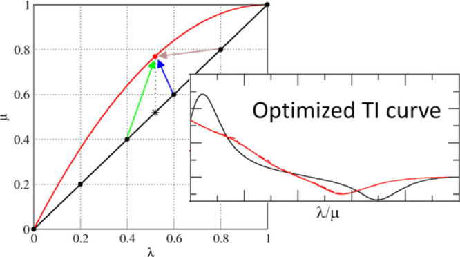
Thermodynamic integration (TI) is a commonly used method to determine free-energy differences. One of its disadvantages is that many intermediate λ-states need to be sampled in order to be able to integrate accurately over ⟨∂H/∂λ⟩. Here, we use the recently introduced extended TI to study alternative parameterizations of H(λ) and its influence on the smoothness of the ⟨∂H/∂λ⟩ curves as well as the efficiency of the simulations. We find that the extended TI approach can be used to select curves of low curvature. An optimal parameterization is suggested for the calculation of hydration free energies. For calculations of relative binding free energies, we show that optimized parameterizations of the Hamiltonian in the unbound state also effectively lower the curvature in the bound state of the ligand.

Introduction

The calculation of free-energy differences is one of the main reasons to perform molecular dynamics (MD) simulations. A prominent example is the determination of thermodynamic properties of small molecules or the (relative) binding affinities of small molecules binding to a common receptor. Amazing progress was made over the years because of a massive increase in available computing power and because of the establishment of powerful methods and protocols. However, the efficiency of free-energy calculations is still limited because of the necessity to capture not only enthalpic but also entropic effects.¹⁻⁴

In alchemical free-energy methods, the free energy between two states or Hamiltonians (H^A and H^B) is computed by combining these using a coupling parameter λ. Different parameterizations of the λ-dependent Hamiltonian [H(λ)] are possible as long as the end states are correctly defined. A common convention is to ensure that at λ = 0, H(λ) = H^A and at λ = 1, H(λ) = H^B. Within this convention, there is a great deal of flexibility to form H(λ), with various approaches being proposed.⁵⁻⁸ Optimal, minimum variance pathways can be derived from theoretical considerations,^9,10 but these may still suffer from kinetic inefficiencies because of large energy barriers in H(λ). In the context of thermodynamic integration (TI),¹¹ an optimal pathway shows the longest thermodynamic length^12,13 or the lowest curvature of ⟨∂H/∂λ⟩ as a function of λ.

The GROMOS simulation package offers quite some flexibility in the parameterization of H(λ) that has not been explored extensively.⁶ Furthermore, we have recently introduced the concept of extended TI, where ⟨∂H/∂λ⟩ at values of λ that were not simulated may be predicted accurately from data stored during the MD simulations using an ensemble reweighting approach.¹⁴ In the current work, we will address three questions:

• 1.Can we predict the shape of a TI curve for an alternative parameterization of H(λ)?
• 2.Can we identify a universally applicable optimal parameterization for a specific task, such as the calculation of hydration free energies?
• 3.Can the optimal curve for one perturbation be transferred to similar perturbations in different environments?

GROMOS uses a versatile λ-dependent Hamiltonian for the nonbonded interaction, in which the alchemical coupling of states A and B and the strength of the soft-core interactions at intermediate λ values can be tuned individually for Lennard-Jones (LJ) and electrostatic (Coulomb with reaction field) interactions. This is done by defining individual coupling parameters, μ_x, that depend on λ through a fourth-order polynomial^15,16

1

with user-specified parameters a_x, b_x, c_x, d_x, e_x.

Using four independent coupling parameters for the nonbonded interactions, μ_lj, μ_slj, μ_crf, and μ_scrf, allows us to write the nonbonded interactions as

2

3

where n is the power dependency of the perturbation, which can additionally be set to any positive integer value, and r_ij is the distance between atoms i and j.

The parameters μ_slj and μ_scrf control the soft-core interaction as

4

5

with C12, C6, and q being the nonbonded force field parameters; α_lj and α_crf, the relevant soft-core parameters; C126_ij^X = C12_ij/C6_ij^X; and C_rf and R_rf, parameters of the reaction-field contribution for long-range electrostatic interactions. While the individual λ-values have been implemented in the GROMOS software for some time already,^15,16 a very similar approach was recently discussed for the AMBER software.^8,17

When using extended TI,¹⁴ the relevant terms of V_LJ, V_CRF and their derivatives with respect to μ_slj and μ_scrf are calculated on the fly during the simulation and stored for a large number of discrete values of μ_slj and μ_scrf. This allows us to compute V_LJ and V_CRF and their derivatives with respect to λ a posteriori for values of λ, other than the simulated λ-points, indicated by λ_s. We will indicate λ-values that are not simulated as λ_p. A simple reweighting equation can subsequently be used to obtain the ensemble averages of the derivative of the Hamiltonian with respect to λ at any λ_p

6

So far, the versatility of the precalculated terms to construct Hamiltonian derivatives has been used to interpolate the derivative between a (sparse) set of simulation points.^14,18,19 However, we can also use these equations to predict ⟨∂H/∂λ⟩ for different individual μ parameter sets or different power dependencies of μ (n in eqs 2 and 3). Because these parameter sets can have a strong influence on the shape of the TI curve, the extended TI predictions can be used to search for TI curves with low curvature. The lower the curvature, the fewer the λ-points required to integrate the curve accurately, which in turn could enhance the efficiency of the simulations. In addition, large peaks in the free-energy curves can indicate that a physical barrier needs to be overcome during the simulation. A smoother free-energy profile will hence also lead to more efficient sampling of the physical degrees of freedom.

Here, we study the influence of the individual parameter sets for the soft LJ interactions (μ_slj) and the soft Coulomb-reaction field interactions (μ_scrf) as well as n. We will first investigate how well we can predict TI curves for other individual sets of μ_x from a short initial simulation. Then, we will try to find a single optimal parameter set for simulations in which atoms are perturbed to dummy atoms (to calculate, for example, hydration free energies). Finally, we show how the optimal λ-dependencies for a simpler system (e.g., perturbation of ligands in solution) can be used for the same perturbation in a more complex system (e.g., perturbation of ligands in the bound state). We will use several test systems, ranging from a very simple methanol to dummy perturbation, up to several post-translational modifications of peptides bound to plant homeodomain (PHD) fingers.

Methods

Using Extended TI to Predict Flatter Curves

The GROMOS simulation package currently supports individual coupling parameters (μ_x) for 12 interaction types. Here, we will only modify the coupling parameters μ_slj and μ_scrf. All other interaction types are simulated with the trivial setting of μ_x = λ. We have previously shown that extended TI is able to accurately predict the complete TI curve based on only a few simulated λ-points.¹⁴ In the first part of this study, we will investigate how accurately extended TI can predict the TI curve for a different μ parameter set. Subsequently, we will investigate how transferable an optimal set of μ_slj and μ_scrf is between molecules or between environments of a single molecule. Initial simulations are performed with the default setting of μ_slj = μ_scrf = λ (set 1). Furthermore, for the initial tests, we assigned two other parameter sets (sets 2 and 3), as shown in Table 1. The latter two sets were chosen based on the following criteria:

• 1μ_x = 0 at λ = 0 and μ_x = 1 at λ = 1, which ensure the same end states for all parameter sets, which allow for a comparison between the final free-energy differences.
• 2μ_scrf should have a smaller derivative at low λ-values than set 1 in order to reduce the typical large peak in the TI curve at low λ-values.
• 3similarly, μ_slj should have a larger derivative at low λ-values because most of the work is normally done at larger λ–values.

Table 1. Selected Individual Parameter Sets, According to eq 1.

set	μx	ax	bx	cx	dx	ex
1	μslj	0.0	0.0	0.0	1.0	0.0
	μscrf	0.0	0.0	0.0	1.0	0.0
2	μslj	0.0	0.0	–0.5	1.5	0.0
	μscrf	0.0	0.0	0.5	0.5	0.0
3	μslj	0.0	0.0	–1.0	2.0	0.0
	μscrf	0.0	0.0	0.7	0.3	0.0
4	μslj	0.7	–1.3	–0.2	1.8	0.0
	μscrf	–0.6	0.9	0.4	0.3	0.0

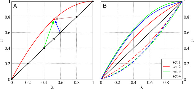
Figure 1B shows how μ_slj and μ_scrf for all sets in Table 1 depend on λ. Furthermore, in the initial tests, we consider both n = 1 and n = 2. Together with the 3 sets of individual μ parameter sets, this results in 6 different simulation settings and 30 predictions that can be made to different parameter sets. For subsequent analyses, we generated a large set of μ_slj and μ_scrf dependencies. For this, we used the conditions that each of a_x, b_x, c_x, and d_x should have a value between −2 and 2.

Figure 1.

Examples of individual μ parameter sets and selection of λ_s-points used to predict at λ_p in different prediction methods. (A) Shown are set 1 (black line) and μ_slj of set 3 (red line), as described in Table 1. The red dot can be predicted in multiple ways from the black line. For the vertical prediction, the green and blue arrows are used (thus, λ_s = 0.4 and 0.6). Maxcont predictions rely on the prediction at the λ_s-point with the most contributing frames (brown arrow). (B) All curves for the sets in Table 1. The solid lines show μ_slj, and the dashed lines show μ_scrf^..

Allowing changes in steps of 0.1, we have found a total of 11,177 sets which satisfy criterion 1. Because not all possibilities will be able to be tested within reasonable time and keeping in mind that many of these sets will result in rather similar relation between λ and μ, we have selected a diverse subset of 1075 sets of μ_slj and μ_scrf. Four of them are given in Table 1, and the rest of them are listed in Table S1 of the Supporting Information.

Extended TI as described in ref (14) makes use of a linear weighting scheme to predict the ⟨∂H/∂λ⟩ at λ_p from the two neighboring λ-points (λ_s1 and λ_s2)

7

where w_s1 and w_s2 are the weighting factors for the simulations at λ_s1 and λ_s2, respectively. The final predicted ⟨∂H/∂λ⟩ value is then determined with

8

In cases where there are no individual μ parameters (i.e., μ_X = λ for all interaction types X), this scheme works well because the smaller the differences between the simulated and predicted λ-points are, the more likely it is that relevant configurations for λ_p are being sampled. However, when there are individual μ parameters, other simulated points which are further away in the λ-space might sample more relevant conformations for the prediction of ⟨∂H/∂λ⟩ at λ_p (see Figure 1A). An alternative scheme would therefore be to predict directly from the simulation that shows the largest number of relevant conformations for the predicted state. For this, we determine the number of contributing frames to the ensemble average in eq 6 by counting the number of configurations for which

9

The simulation which shows the largest number of contributing frames will then be used to determine ⟨∂H/∂λ⟩_λp. Note that in this case, λ_s does not have to be one of the neighboring λ-points of λ_p (e.g., following the brown arrow in Figure 1A). Additionally, predictions can be calculated using weighted average over all simulations, according to the number of contributing frames.

Simulation Settings

Several test systems are used in this study. Initial tests were performed for perturbations of methanol to a noninteracting dummy molecule in water. Subsequently, we expanded the set to compute the hydration free energies of p-xylene, cyclopentanol, undecane, and phenol. Finally, we performed relative free-energy calculations between different histone tail molecules, binding to PHD fingers, involving perturbations from glutamine to serine (GLN_SER), lysine to N6,N6,N6-trimethyl-lysine (LYSH_K3C), and lysine to N-acetyllysine (LYSH_KAC). All simulations are performed with the GROMOS11 simulation package (version 1.5.0),²⁰ in combination with the GROMOS force field 54a8.²¹ Cubic simulation boxes are used, which are filled with SPC water molecules.²² Simulations are performed at a temperature of 300 K (298 K for aspirin) by weakly coupling²³ it to an external bath with a coupling time of 0.1 ps. Solute and solvent degrees of freedom are coupled to separate baths. The pressure is kept constant at 1 atm by isotropic weak coupling²³ with a relaxation time of 0.5 ps and a compressibility of 7.624 × 10^–4 (kJ mol^–1 nm^–3)⁻¹ for methanol, phenol, p-xylene, cyclopentane, and undecane and a compressibility of 4.575 × 10^–4 (kJ mol^–1 nm^–3)⁻¹ for aspirin and the perturbations GLN_SER, LYSH_K3C and LYSH_KAC in each of the environments. The center of mass movement of the solute is removed every 1000 steps. Nonbonded interactions up to 0.8 nm are calculated at every time step from a pair list that is updated every 10 fs. Interactions up to 1.4 nm are calculated at every update of the pair list and kept constant in between. A reaction-field contribution is added to the electrostatic interactions and forces to account for a homogeneous medium with a dielectric permittivity of 61 (78.5 for phenol, p-xylene, cyclopentanol, and undecane) outside the cutoff sphere.²⁴ The SHAKE algorithm²⁵ is used to constrain bond lengths to their optimal value. In the methanol, GLN_SER, LYSH_K3C, and LYSH_KAC simulations, SETTLE was used to constrain the solvent bond lengths.²⁶

Softness parameters for atoms that are being perturbed are set to α_LJ = 0.5 and α_CRF = 0.5 nm². The power dependence n is generally set to 1 unless stated otherwise. For extended TI, the number of precalculated λ-points is set 101. The precalculated energy and free-energy terms are written to file every 0.1 ps.

The perturbations GLN_SER, LYSH_K3C, and LYSH_KAC are performed based on a dual-topology approach, within multiple environments, within a pentapeptide (GGXGG), within a histone tail peptide, and within a histone tail peptide which is bound to a PHD finger. Initial coordinates for the histone tail peptides in the complex with the PHD fingers are obtained from the PDB database with identifiers 5FB0 (LYSH_K3C),²⁷ 5WXH (LYSH_KAC),²⁸ and 5FB1 (GLN_SER).²⁷ The histone tail peptides as present in the complexes consist of 7–10 amino acids. In the complexes, there are two Zn²⁺ ions present which are kept in place by distance restraints to the coordinating residues.

Results and Discussion

Accuracy of Predictions for Other Individual μ Sets

The methanol-to-dummy atom transformation is used as the first test system to determine how well the TI curve can be predicted for alternative μ parameter sets with extended TI. In particular, this transformation was performed with individual μ parameter sets 1, 2, and 3 (see Table 1) for the μ power dependence (n) equal to 1 and 2. The profiles of ⟨∂H/∂λ⟩_λp for each of these reference simulations are given in Figure 2. It can be seen that sets 2 and 3 lead to curves with less curvature than set 1 and can be expected to be integrated more readily. In order to have a more quantitative measure of the smoothness of the curve, we determine the average curvature by calculating the numerical second derivative of ⟨∂H/∂λ⟩_λp and averaging over its absolute value.

Figure 2.

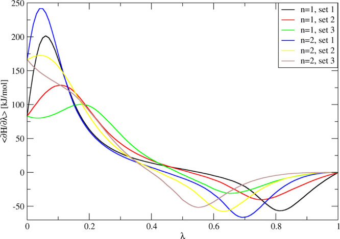
Six ⟨∂H/∂λ⟩ curves for three sets and two values of n for perturbations of methanol in water to noninteracting dummy atoms. Simulations are performed for 5 ns at 21 λ-points.

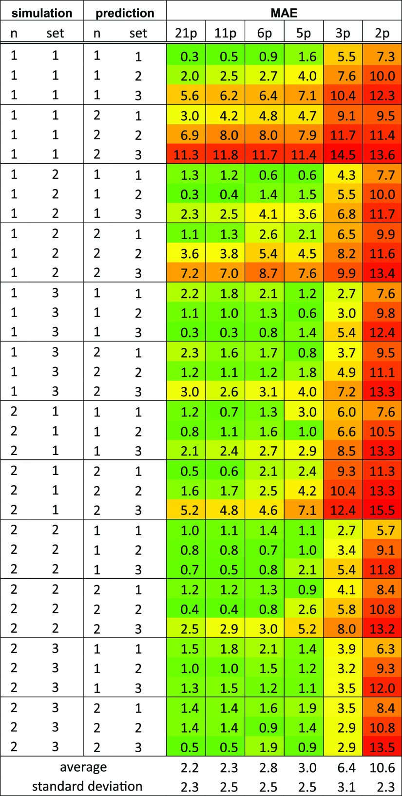
From each of the simulations, predictions are made to each of the other sets and for comparison, also without changes in the parameter sets. The performance of the predictions is measured in terms of the mean absolute error (MAE) over the entire curve (101 λ_p values), with respect to the reference simulation. The reference data are in these cases obtained from 5 ns simulations at 21 equidistant λ-points, with extended TI to predict the curve between the simulated points. Note that the MAE over the curve is a more stringent criterion than just using the deviation in the final free energy (see Table S2) because there, a cancellation of errors may occur. On average, the deviations in the total free energies are indeed lower than the averages of the MAE, especially when only a few λ-points are used. In many cases, they are quite similar, but in some cases, the predictions can appear to be very good with, for example, a final free-energy deviation of 1.1 kJ/mol, but an MAE of 12.0 kJ/mol (simulated with n = 2, set 3, prediction for n = 1, set 3 based on only 2 λ-points). For this reason, we continue our analysis based on the MAE.

Table 2 shows the results when using 2 up to 21 equidistant λ-points to predict the whole curve using the linear weighting scheme. Note that the predictions are based on 1 ns simulations, whereas the reference data are based on 5 ns simulations. Therefore, even for predictions made for the same set and n value, an MAE larger than 0 is obtained for the 21-point column. The 21-point column is an indication if we can achieve a good prediction of the results from one parameter set to another at all, without optimizing the efficiency. This shows, for example, that it is very difficult to predict directly from set 1 to set 3 without changing the power dependence. Even with 21 λ-points, the MAEs are 5.6 and 5.2 kJ/mol for n = 1 and n = 2, respectively. On the other hand, predicting set 1 from set 3 with 21 λ-points appears to work better, with MAEs of 2.2 and 1.4 kJ/mol for n = 1 and n = 2, respectively. Although the difference is less pronounced, a similar trend is observed for the predictions of set 2 from set 1 and vice versa as well as for set 3 from set 2. It appears that the prediction of a curve with lower average curvature is more difficult than predicting a higher-average-curvature curve.

Table 2. MAE for Prediction between Different Parameter Sets and Power Dependencies Using a Range of Number of λ-Points (21 to 2 Points)^a.

^aVertical predictions based on 1 ns and reference simulated for 5 ns and 21 points.

Also, for changing just the power dependence, it depends in which direction the change is predicted. Predicting n = 2 from n = 1 results in MAEs between 3.0 and 3.6 kJ/mol for the three sets, whereas the other way around, very low MAEs of 0.8–1.3 kJ/mol are reached.

Table 2 also gives an indication of how many λ-points are necessary to give a reasonably accurate prediction. It is especially useful to compare the MAE obtained with a certain number of λ-points to the result using all 21 λ-points. We see that using six λ-points, the MAEs are only slightly larger than the results with 21 λ-points. Upon reducing to five λ-points, most results stay rather similar, but there are a few exceptions. The largest difference in MAE between predictions from six and five λ-points is 2.5 kJ/mol for the prediction from n = 2, set 1 to n = 2, set 3. For this reason, from now on, six λ-points will be simulated to predict the results for other parameter sets.

Predictions Based on the Maximum Number of Contributing Configurations

Because it appears more difficult to predict curves with lower curvatures from higher-curvature ones, we need to find a way to optimize our predictions. So far, we have used a linear weighting scheme to predict the TI curves for other λ parameter sets, which we will call vertical predictions. Figure 1A shows two examples of λ parameter sets. The black and red lines show the behavior of μ_slj with respect to λ for sets 1 and 3, respectively. In this example, we assume that we have simulated six equidistant λ-points with set 1 and want to predict set 3 from this. For example, when predicting λ_p = 0.52 (red dot), we would in principle predict this from λ_s = 0.52, as indicated by the vertical dotted line and its star on the black line. However, because simulations are only performed at six equidistant λ-points, a linear combination of the predictions at the surrounding λ_s-points is used as indicated by the green and blue arrows in Figure 1A. Note that these λ_s-points only depend on λ_p and are independent of the individual parameter set.

Another possibility to predict TI curves is by taking the prediction from the simulated λ-point that shows the largest number of configurations that contribute to the ensemble averages on the right-hand side of eq 6. The number of contributing configurations is determined using eq 9. Assuming that the λ_s-point which has the most contributing configurations for λ_p is also the one which gives the most accurate prediction at λ_p, this prediction is directly used, without any linear scaling. We refer to this approach as the Maxcont method. In order to test if a higher number of contributing frames also correspond to a more accurate prediction, we plot the number of contributing frames versus the absolute error at each of the predicted λ-points with respect to the reference data. Figure 3 shows this analysis for the simulation of the methanol-to-dummy transformation with n = 2 and set 1. Predictions are made based on six equidistant points for the same set (black dots), set 2 (red dots), and set 3 (green dots). Although there is no direct linear dependence, there is a clear trend that with a large enough number of contributing frames, the absolute errors at each λ-point are small.

Figure 3.

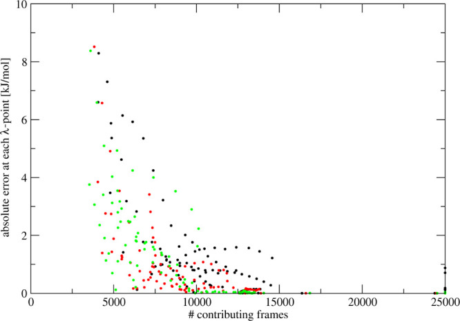
Absolute error at each λ-point from predictions based on the maximum number of contributing frames for the methanol-to-dummy transformations. Predictions are made for n = 2, set 1 (black dots), set 2 (red dots), and set 3 (green dots) based on a 1 ns simulation at six equidistant points of n = 2, set 1. These predictions are compared to the simulations of each of the sets at 21 equidistant λ-points and 5 ns simulations.

The predictions from the simulated λ-points which had the largest number of contributing snapshots (red squares in Figure 4) are overall very good. Not only changes between parameter sets but also changes in the power dependence or a combination of both are very well predicted with this method. The largest MAE obtained in any of the combinations is only 2.0 kJ/mol and the average is 1.3 kJ/mol. Similar trends are observed when the deviations in the final free energies are evaluated (see Figure S1). Furthermore, we have tested a hybrid scheme in which predictions from different λ_s-points are used in a weighted average, according to the number of contributed frames, where all simulations were taken into account. Figure S2 shows that such an approach does not improve the predictions because really bad predictions still get included in the weighted average. These results show that at least for this test system, the Maxcont prediction method is the most reliable one. A disadvantage of the Maxcont predictions is that sudden “jumps” can occur in the predicted curves, when for two neighboring λ_p-points, different λ_s-points are used. We will apply two measures in order to smoothen these jumps. The first case that we address is when only a single λ_p-point (e.g., 0.73) uses a different λ_s-point [e.g., λ_s (0.73) = 0.80] from the surrounding λ_p-points [e.g., λ_s (0.72) = λ_s (0.74) = 0.60]. Even though the number of contributing frames was higher for the alternative λ_s-point, we then use the prediction based on λ_s (0.73) = 0.60. This leads to a much smoother prediction and mostly likely a more accurate one. The second measure that we take is to use a running average over five points before calculating the average curvature of the predicted curves.

Figure 4.

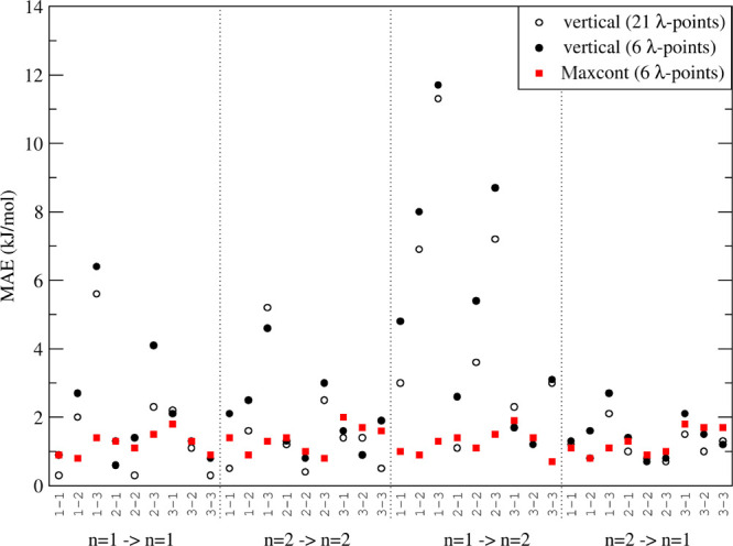
MAEs for predictions between sets as indicated on the x-axis. Predictions are based on simulations at 21 or 6 λ-points using the vertical or Maxcont approaches (see the text).

Optimal Set for Hydration Free Energies

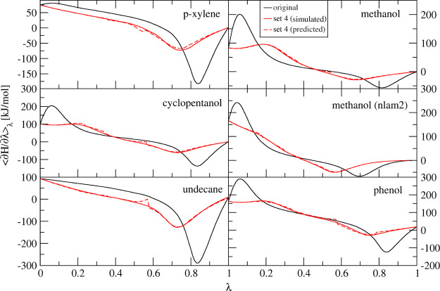
During our investigations, we have found that for systems in which atoms are turned into dummy atoms, a single set of λ-dependencies for μ_slj and μ_scrf can be used, which improves the smoothness of the free-energy curve significantly. The test systems included here are phenol, methanol (n = 1), methanol (n = 2), p-xylene, cyclopentanol, and undecane. In Figure 5, the original free-energy curves (black lines) have two kinds of shapes in these test systems. First, we have the undecane and p-xylene curves where there is only a deep well at around λ = 0.85. These two systems have no (undecane) or only very small (p-xylene) partial charges. The minimum in the free-energy curve thus comes from the vdW contributions. The other test systems contain larger partial charges and show an additional peak around λ = 0.05. Most test systems were simulated with n = 1, and only methanol was additionally simulated with n = 2. The most obvious difference between these two free-energy curves is that with n = 2, the minimum is shifted toward a smaller λ-value (around 0.7).

Figure 5.

Free-energy profiles for perturbations of various molecules into dummy atoms. Black lines: original set, 21 points, 5 ns. Solid red line: simulated with set 4; 21 λ-points, 5 ns. Dashed red line: prediction of optimized from original using Maxcont (based on simulations using set 1 at six λ-points, 1 ns). Unless stated otherwise, all simulations are simulated with n = 1.

The shapes of the curves as shown in Figure 5 are very typical for GROMOS free-energy calculations where real atoms are perturbed into dummy atoms. It is possible to get different shapes though, for example, with different softness settings and even higher values of n.^5,6

Because of the similar shape in each of these cases, we investigated if there is a single set of λ-dependencies for μ_slj and μ_scrf which can help smoothen the curves for all these test systems. For this, we tested 1075 combinations of μ_slj and μ_scrf for each of the test systems. The predictions are based on 1 ns of simulation at six equidistantly spaced λ-points, and the average curvature is computed as described above. After sorting all the predictions based on their average curvature, we found one set (set 4 in Table 1) which was among the top ranked ones for each of the six test systems. We then continued to simulate the test systems with this new set of λ-dependencies for μ_slj and μ_scrf in order to find out if the predictions were accurate. Figure 5 shows the TI curves obtained from simulations with the original set from the predictions for set 4 and from explicit simulations with set 4. The MAE between the predicted and simulated curves ranges between 0.9 (methanol, n = 2) and 3.0 kJ/mol (phenol). Mostly, the difference between the predicted and simulated curves comes from the usage of the Maxcont approach to combine the predictions from each λ_s-point, with sudden irregularities in the curves. The final free-energy differences (Table S3) show very similar values for the each of the sets. Mostly, the deviations between set 1 and set 4 (both the predictions and simulations) do not exceed 0.8 kJ/mol. The only exception is for cyclopentanol, where the difference between the simulated data using set 1 and predictions for set 4 (based on simulations of set 1) is 2.3 kJ/mol.

Now that we have identified a set of μ_slj and μ_scrf which results in curves with lower curvature, we should confirm if the convergence between the original and optimized sets improved. For this, we will mimic an adaptive simulation scheme, adding more data sequentially until a convergence criterion has been met. We will start from 6 λ_s-points, each simulated using set 1 or 4 for 0.5 ns, from which the entire curve over 101 λ_p-points is predicted. If for any value of λ_p, a preset minimum of contributing frames (eq 9) is not reached, the simulations at the corresponding λ_s-points will be prolonged for another 0.5 ns, with a maximum of 5 ns overall simulation time per λ_s-point. As a minimum number of contributing frames, we used 10,000 and 15,000 configurations. Once internal consistency is reached in this way, the curve is compared to the reference curve, computed from 21 λ_s-points of 5 ns each, and the MAE is calculated.

The results can be found in Figure 6. In general, convergence is reached faster with set 4 as opposed to set 1. The actual efficiency gain is system-dependent and also threshold-dependent. Note that for undecane, convergence was not reached using set 1 within the maximum of 5 ns per λ_s-point. Alternative convergence criteria can be devised, for instance, based on an average bootstrap error in the free-energy differences (Figure S3) or based on other predictors (Petrov et al., in preparation). While the convergence behavior is different using different criteria, both approaches tested here agree that set 4 is more efficient than set 1.

Figure 6.

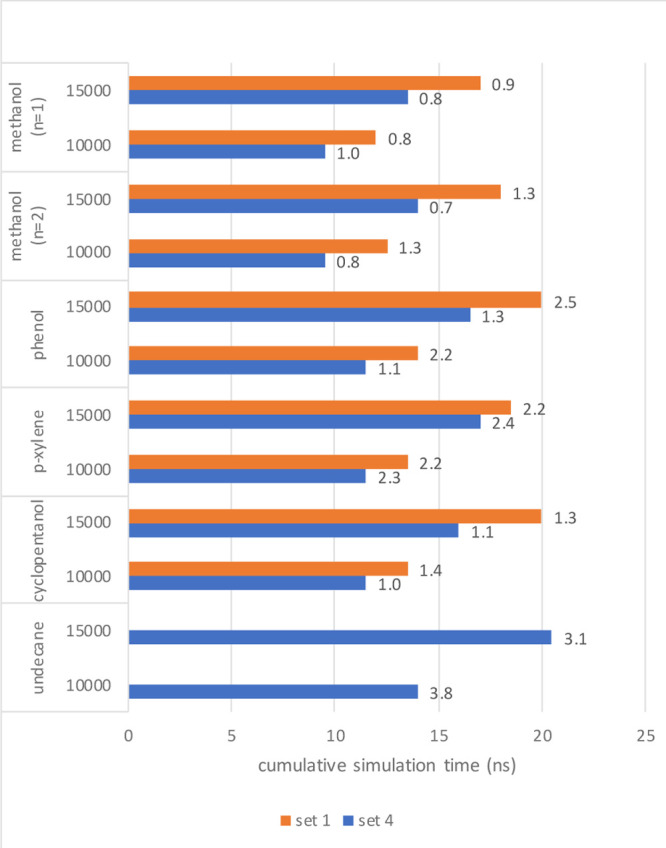
Result from convergence analysis; total simulation time required to reach convergence based on the minimum number of contributing frames of 10,000 or 15,000 for simulations for set 1 (orange) and set 4 (blue). When no bar is shown, convergence was not yet reached (with a maximum simulation time of 5 ns per λ-point). The value on the right side of the bars gives the MAE (in kJ/mol) of the converged simulation with respect to the reference data (21 λ-points for 5 ns).

It is important to establish in which cases, set 4 will give the smoothest curves. For example, the simulations will need to be performed with α_lj = 0.5 and α_crf = 0.5 nm² and n should be equal to 1 or 2. We also have to keep in mind that with set 4, the LJ interactions are removed faster than the electrostatic interactions (Figure 1B). This can become problematic if there are, for example, counterions present in the simulation box. The counterion might be attracted to some (still) partially charged atoms which do not have much LJ interactions left. In this case, the counterion can collapse on top of these atoms, causing very large fluctuations in the free energies. This can be shown on the more challenging system of the negatively charged aspirin. Because of the negative charge, a positively charged Na⁺ ion is added to simulation as a counterion. The perturbation to dummy atoms is performed, similar to the other systems of this section. After performing the predictions of the 1075 sets, we find that set 4 is not the most optimal set but still relatively highly ranked. However, performing the simulations with set 4, we see that the problem as described above occurs. In the range of λ = 0.2 up to λ = 0.4, very large jumps occur in the TI curve (Figure S4A). Further analysis showed that at λ = 0.3, the Na⁺ ion moves directly on top of the oxygen atom of the carboxyl group (see Figure S4B). Performing the simulation again with set 4 but now without the counterion, we obtain a TI curve which is very similar to the originally predicted curve for set 4 (Figure S4A). Similar behavior can occur for ligands bound to a protein, so set 4 is predominantly recommended for the calculation of hydration free energies.

Optimal Set for Simulations in Water Can be Transferred to the System in Protein

In the section above, one particular type of perturbation was analyzed (real atoms to dummy atoms), for which the contribution of V_LJ and V_CRF can be readily assigned to the regions of high curvature in the original TI profile and a more optimal set of interactions can be selected. In other types of perturbations, these LJ and CRF contributions may look very differently. A prominent example in the field is the calculation of the relative binding free energy between two rather similar molecules to a protein. Perturbing one molecule into the other can include change of atom types, change of partial charges (even sign changes), growing in atoms, and removing atoms. In addition, there might be changes in the bond lengths, angles, etc., but in the current examples, we will focus on a dual-topology approach, in which only nonbonded interactions contribute.

Because of the large amount of possibilities, we will not be able to find a general optimized set of μ_x-values for any type of perturbation. However, we take advantage of the fact that usually the same perturbations are performed once in solution and once in a bound state. Both perturbations are typically very similar but influenced by their surroundings. We might be able to optimize the perturbation in solution and use this for the simulations in the bound state. This implies that we can avoid performing an initial simulation of the computationally more intense bound state before finding an optimized set.

We will test this hypothesis with some post-translational modifications (PTMs) of histone tail peptides in water and bound to PHD fingers. As a possible further optimization, we will perform the PTMs in a pentapeptide (GGXGG). This would allow us to generate an optimal individual λ-dependency for μ_slj and μ_scrf for a certain PTM, which can then be applied to any peptide or protein.

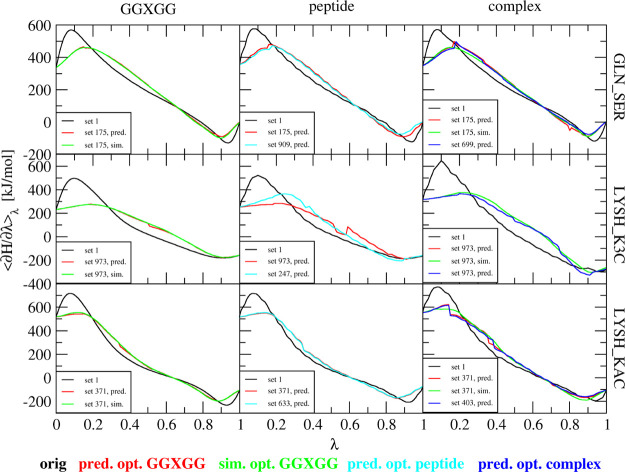
The side-chain modifications that will be investigated include GLN - > SER, LYSH - > K3C (N6,N6,N6-trimethyllysine), and LYSH - > KAC (N-acetyllysine). The perturbations of the histone tail peptides in water are performed for 5 ns at 21 λ-points. We subsequently used 1 ns of simulation at 6 λ-points to predict the TI curves for the same 1075 individual μ_slj and μ_scrf sets as used in the previous section (Table S1). Figure 7 shows the resulting TI curves. In black, the original curves with set 1 (Table 1) are given. The red curves are predicted from the original simulations using the set of μ_slj and μ_scrf that leads to lowest curvature in the GGXGG system. The green curves show the resulting curves when this set was simulated. The cyan and blue curves show predictions from the original simulation using sets of μ_slj and μ_scrf that lead to lowest average curvature in the peptide or in the complex simulations, respectively. All the optimal λ-dependencies for μ_slj and μ_scrf are shown in Figure S5 in the Supporting Information.

Figure 7.

Free-energy profiles for three different perturbations in three different contexts using different parameterizations of the Hamiltonian. Black lines: simulations with set 1 with 21 λ-points for 5 ns. Red lines: predicted curves with the optimal set based on the GGXGG simulation. Green lines: simulations with the optimal set based on the GGXGG simulation performed at 11 equidistance λ-points for 1 ns. Cyan lines: predicted curves with the optimal set based on the peptide simulation. Blue lines: predicted curves with the optimal set based on the complex simulation. All predictions are based on 1 ns simulations at equidistant six λ-points.

GLN_SER

GLN_SER is a challenging test case because quite large partial charges appear and disappear during the perturbation. This implies that peaks due to the electrostatic contributions will occur at both small and large λ-values. Searching for an optimal λ-dependency for μ_scrf would thus require an s-like shape such that the work is shifted toward the middle of the curve. Starting with the peptide in solution, we found that set 909 has the lowest average curvature of all the tested possibilities. In the case of the pentapeptide, we found a different optimal set 175, but the predicted curves for these two sets are very similar. Predicting the optimal set from the complex resulted in set 699. The complex was then simulated with the optimal set as predicted by the GGXGG system. Note that the peak at low λ-values is not completely flattened out, but overall, this curve has a similar curvature as the optimal set for the complex (699; in blue).

LYSH_K3C

The challenge of this test system is that three methyl groups are grown during the perturbation. The optimal predicted set based on the GGXGG simulations is set 973. The peak at low λ-values is almost completely flattened out with this set. For the peptide simulation, the predicted optimal set was set 247. In this case, the first peak is a bit lower and slightly shifted toward λ = 0.3. Looking into set 973, which was performing so well for the GGXGG system, we find that in the peptide simulation, this set was ranked #284. The average curvature is so much higher in this case because of two sudden jumps close to λ = 0.5 and 0.6. These jumps are a result of the Maxcont scheme which is used here, where two neighboring λ-points are predicted from two different λ_s-points. Although this is an indication that the prediction might be more uncertain, this kind of jump would not be expected when simulations are performed with this set. Predicting the optimal set from the simulation of the complex resulted in set 973. This is actually the same optimal set as that obtained from the GGXGG simulations. A simulation using this set indeed leads to a very comparable profile.

LYSH_KAC

In this perturbation, an acetyl group replaces one of the hydrogens of the amino group of lysine, which includes a charge change from +1 to 0. From the GGXGG simulations, set 371 was predicted to have the lowest average curvature. Predictions from the simulations of the peptide and the complex resulted in the optimal sets of 633 and 403, respectively. As shown in Figure 7, all three sets result in very similar predictions. This is also represented in the ranks of the predicted sets based on their average curvatures. All 3 sets are within the top 10 for each of the system sizes. The simulated curve using the optimal parameters for the GGXGG system is very similar to the predicted curves using individually optimized sets for μ_slj and μ_scrf.

Table S4 shows the final free-energy differences for each of the free-energy profiles shown in Figure 7. For the GLN_SER system, the free-energy differences are very close to each other for each of the respective system sizes. The largest deviation occurs in the pentapeptide, where the original set results in 205.6 kJ/mol, whereas the prediction with the optimal set results in 208.3 kJ/mol. The results for the LYSH_K3C system show relatively consistent free-energy differences for the pentapeptide and the peptide system (with a maximum deviation of 3.2 kJ/mol). However, for the complex system, there is a large discrepancy between the simulation of set 1 (87.3 kJ/mol) and the simulation with the optimal set as obtained from the pentapeptide system (106.2 kJ/mol). This could be due to the short simulation time of 1 ns with the optimal set from the pentapeptide system, but it could also be an indication that the sampling of the physical degrees of freedom is more efficient for the curve with lower curvature and the final free energy with this smoother curve is more appropriate. The final free-energy differences for the LYSH_KAC systems again show lower deviations between the different sets. The largest deviation is found in the complex between set 1 (190.6 kJ/mol) and the prediction with the optimal set obtained from the pentapeptide (187.1 kJ/mol).

As was shown above, there is no single optimal set of λ-dependencies for μ_slj and μ_scrf which can be applied to all types of perturbation. However, it is possible to optimize it for a particular perturbation in a small system (single ligand or, for example, pentapeptide in the case of amino acids) and subsequently use this optimized set for the same perturbation in a large system (e.g., the complex of ligand/peptide and protein). This provides a significant improvement of efficiency because the complex only has to be simulated with the optimized set of parameters. Even more efficiency is gained in the case of the perturbation of amino acids because it appears that they can be optimized independent of their surroundings. Thus, one can derive one optimal set for each of the 20 × 19 = 380 potential mutations in a pentapeptide of the form GGXGG which can subsequently be used for any other protein or peptide system.

Conclusions

During this study, we have looked at alternative μ parameter sets for the calculation of free-energy differences with extended TI. Initial tests on the simple methanol system showed that only short (e.g., 1 ns long) initial simulations at six equidistant λ-points are enough to reliably predict the ⟨∂H/∂λ⟩ curves for other parameter sets by applying the Maxcont scheme. All possible combinations of three μ parameter sets and two values of n resulted in a maximum MAE of 2 kJ/mol between the reference simulations and its predictions. Knowing that we can predict the shape of the ⟨∂H/∂λ⟩ curves for other parameter sets rather well, we turned to testing many possible parameter sets on a few selected systems in which all atoms are turned into dummy atoms. From this large pool of 1075 sets, we have found set 4, which resulted in a predicted curve with low average curvature for each of the systems. This set can be expected to work well for other systems where atoms are turned into dummy atoms, which should then require less λ-points to integrate accurately. Note that there would be a much larger gain in efficiency if regular TI would be used because extended TI already provides a more accurate integration because of its predictions between the simulated λ-points.

The last part of this study involved relative binding free energies which are typically more challenging because of the more diverse shapes of ⟨∂H/∂λ⟩ curves. Analysis of these more complex perturbations showed that in contrast to the hydration free energy example, there is no general optimal set for any perturbation. We did, however, find that for each perturbation, we can optimize the parameter set based on the simulations in a simple system with a small simulation box (such as a pentapeptide in water) which can then also be applied to larger and more complex systems (such as a peptide–protein complex). This removes the necessity for initial simulations of the large system. Overall, we find that the use of extended TI does not only lead to smoother curves to integrate but also allow for an efficient means to test for different parameterizations of the λ-dependent Hamiltonian and to obtain low-curvature free-energy profiles.

Supporting Information Available

The Supporting Information is available free of charge at https://pubs.acs.org/doi/10.1021/acs.jctc.0c01170.

• Absolute errors in ΔG for the data; use of a weighted Maxcont approach; convergence behavior when using a bootstrap criterion; results for the aspirin simulations; λ-dependency of μ_slj and μ_scrf for all optimal sets mentioned in the PTM section; list of sets 5–1075 for the parameterization of μ_slj and μ_scrf; absolute errors in ΔG for the data; and ΔG values for the data (PDF)

The authors declare no competing financial interest.

References

- Chodera J. D.; Mobley D. L.; Shirts M. R.; Dixon R. W.; Branson K.; Pande V. S. Alchemical Free Energy Methods for Drug Discovery: Progress and Challenges. Curr. Opin. Struct. Biol. 2011, 21, 150–160. 10.1016/j.sbi.2011.01.011. [DOI] [PMC free article] [PubMed] [Google Scholar]
- Chipot C. Frontiers in Free-Energy Calculations of Biological Systems. Wiley Interdiscip. Rev.: Comput. Mol. Sci. 2014, 4, 71–89. 10.1002/wcms.1157. [DOI] [Google Scholar]
- Cournia Z.; Allen B.; Sherman W. Relative Binding Free Energy Calculations in Drug Discovery: Recent Advances and Practical Considerations. J. Chem. Inf. Model. 2017, 57, 2911–2937. 10.1021/acs.jcim.7b00564. [DOI] [PubMed] [Google Scholar]
- de Ruiter A.; Oostenbrink C. Advances in the Calculation of Binding Free Energies. Curr. Opin. Struct. Biol. 2020, 61, 207–212. 10.1016/j.sbi.2020.01.016. [DOI] [PubMed] [Google Scholar]
- Pham T. T.; Shirts M. R. Identifying Low Variance Pathways for Free Energy Calculations of Molecular Transformations in Solution Phase. J. Chem. Phys. 2011, 135, 034114. 10.1063/1.3607597. [DOI] [PubMed] [Google Scholar]
- de Ruiter A.; Boresch S.; Oostenbrink C. Comparison of Thermodynamic Integration and Bennett Acceptance Ratio for Calculating Relative Protein-Ligand Binding Free Energies. J. Comput. Chem. 2013, 34, 1024–1034. 10.1002/jcc.23229. [DOI] [PubMed] [Google Scholar]
- König G.; Glaser N.; Schroeder B.; Kubincová A.; Hünenberger P. H.; Riniker S. An Alternative to Conventional λ-Intermediate States in Alchemical Free Energy Calculations: λ-Enveloping Distribution Sampling. J. Chem. Inf. Model. 2020, 60, 5407. 10.1021/acs.jcim.0c00520. [DOI] [PubMed] [Google Scholar]
- Lee T.-S.; Lin Z.; Allen B. K.; Lin C.; Radak B. K.; Tao Y.; Tsai H.-C.; Sherman W.; York D. M. Improved Alchemical Free Energy Calculations with Optimized Smoothstep Softcore Potentials. J. Chem. Theory Comput. 2020, 16, 5512. 10.1021/acs.jctc.0c00237. [DOI] [PMC free article] [PubMed] [Google Scholar]
- Reinhardt M.; Grubmüller H. Determining Free-Energy Differences Through Variationally Derived Intermediates. J. Chem. Theory Comput. 2020, 16, 3504–3512. 10.1021/acs.jctc.0c00106. [DOI] [PMC free article] [PubMed] [Google Scholar]
- Pham T. T.; Shirts M. R. Optimal Pairwise and Non-Pairwise Alchemical Pathways for Free Energy Calculations of Molecular Transformation in Solution Phase. J. Chem. Phys. 2012, 136, 124120. 10.1063/1.3697833. [DOI] [PubMed] [Google Scholar]
- Kirkwood J. G. Statistical Mechanics of Fluid Mixtures. J. Chem. Phys. 1935, 3, 300. 10.1063/1.1749657. [DOI] [Google Scholar]
- Naden L. N.; Pham T. T.; Shirts M. R. Linear Basis Function Approach to Efficient Alchemical Free Energy Calculations. 1. Removal of Uncharged Atomic Sites. J. Chem. Theory Comput. 2014, 10, 1128–1149. 10.1021/ct4009188. [DOI] [PubMed] [Google Scholar]
- Naden L. N.; Shirts M. R. Linear Basis Function Approach to Efficient Alchemical Free Energy Calculations. 2. Inserting and Deleting Particles with Coulombic Interactions. J. Chem. Theory Comput. 2015, 11, 2536–2549. 10.1021/ct501047e. [DOI] [PubMed] [Google Scholar]
- de Ruiter A.; Oostenbrink C. Extended Thermodynamic Integration: Efficient Prediction of Lambda Derivatives at Nonsimulated Points. J. Chem. Theory Comput. 2016, 12, 4476. 10.1021/acs.jctc.6b00458. [DOI] [PubMed] [Google Scholar]
- Hritz J.; Oostenbrink C. Hamiltonian Replica Exchange Molecular Dynamics Using Soft-Core Interactions. J. Chem. Phys. 2008, 128, 144121. 10.1063/1.2888998. [DOI] [PubMed] [Google Scholar]
- Riniker S.; Christ C. D.; Hansen H. S.; Hünenberger P. H.; Oostenbrink C.; Steiner D.; van Gunsteren W. F. Calculation of Relative Free Energies for Ligand-Protein Binding, Solvation, and Conformational Transitions Using the GROMOS Software. J. Phys. Chem. B 2011, 115, 13570–13577. 10.1021/jp204303a. [DOI] [PubMed] [Google Scholar]
- Lee T.-S.; Allen B. K.; Giese T. J.; Guo Z.; Li P.; Lin C.; McGee T. D. Jr; Pearlman D. A.; Radak P. K. Alchemical Binding Free Energy Calculations in AMBER20: Advances and Best Practices for Drug Discovery. J. Chem. Inf. Model. 2020, 60, 5595. 10.1021/acs.jcim.0c00613. [DOI] [PMC free article] [PubMed] [Google Scholar]
- Maurer M.; Hansen N.; Oostenbrink C. Comparison of free-energy methods using a tripeptide-water model system. J. Comput. Chem. 2018, 39, 2226–2242. 10.1002/jcc.25537. [DOI] [PMC free article] [PubMed] [Google Scholar]
- Hahn D. F.; Hünenberger P. H. Alchemical Free-Energy Calculations by Multiple-Replica λ-Dynamics: The Conveyor Belt Thermodynamic Integration Scheme. J. Chem. Theory Comput. 2019, 15, 2392–2419. 10.1021/acs.jctc.8b00782. [DOI] [PubMed] [Google Scholar]
- Schmid N.; Christ C. D.; Christen M.; Eichenberger A. P.; van Gunsteren W. F. Architecture, Implementation and Parallelisation of the GROMOS Software for Biomolecular Simulation. Comput. Phys. Commun. 2012, 183, 890–903. 10.1016/j.cpc.2011.12.014. [DOI] [Google Scholar]
- Reif M. M.; Hünenberger P. H.; Oostenbrink C. New Interaction Parameters for Charged Amino Acid Side Chains in the GROMOS Force Field. J. Chem. Theory Comput. 2012, 8, 3705–3723. 10.1021/ct300156h. [DOI] [PubMed] [Google Scholar]
- Berendsen H. J. C.; Postma J. P. M.; Van Gunsteren W. F.; Hermans J.. Interaction Models for Water in Relation To Protein Hydration. In Intermolecular Forces; Reidel: Dordrecht, The Netherlands, 1981; Vol. 11, pp 331–342. [Google Scholar]
- Berendsen H. J. C.; Postma J. P. M.; van Gunsteren W. F.; DiNola A.; Haak J. R. Molecular Dynamics with Coupling to an External Bath. J. Chem. Phys. 1984, 81, 3684–3690. 10.1063/1.448118. [DOI] [Google Scholar]
- Tironi I. G.; Sperb R.; Smith P. E.; van Gunsteren W. F. A Generalized Reaction Field Method for Molecular Dynamics Simulations. J. Chem. Phys. 1995, 102, 5451–5459. 10.1063/1.469273. [DOI] [Google Scholar]
- Ryckaert J.-P.; Ciccotti G.; Berendsen H. J. C. Numerical Integration of the Cartesian Equations of Motion of a System with Constraints: Molecular Dynamics of n-Alkanes. J. Comput. Phys. 1977, 23, 327–341. 10.1016/0021-9991(77)90098-5. [DOI] [Google Scholar]
- Miyamoto S.; Kollman P. A. Settle: An Analytical Version of the SHAKE and RATTLE Algorithm for Rigid Water Models. J. Comput. Chem. 1992, 13, 952–962. 10.1002/jcc.540130805. [DOI] [Google Scholar]
- Zhang X.; Zhao D.; Xiong X.; He Z.; Li H. Multifaceted Histone H3 Methylation and Phosphorylation Readout by the Plant Homeodomain Finger of Human Nuclear Antigen Sp100C. J. Biol. Chem. 2016, 291, 12786–12798. 10.1074/jbc.M116.721159. [DOI] [PMC free article] [PubMed] [Google Scholar]
- Zhao S.; Yang M.; Zhou W.; Zhang B.; Cheng Z.; Huang J.; Zhang M.; Wang Z.; Wang R.; Chen Z.; Zhu J.; Li H. Kinetic and High-Throughput Profiling of Epigenetic Interactions by 3D-Carbene Chip-Based Surface Plasmon Resonance Imaging Technology. Proc. Natl. Acad. Sci. U.S.A. 2017, 114, E7245–E7254. 10.1073/pnas.1704155114. [DOI] [PMC free article] [PubMed] [Google Scholar]
Associated Data
This section collects any data citations, data availability statements, or supplementary materials included in this article.