

Abstract
China is the first major economy to show a recovery after a slowdown induced by the COVID-19 pandemic. This work aims to explore what the China’s economic recovery after the COVID-19 pandemic means for the economic growth and energy consumption of the other countries using the global VAR quarterly data. In the long term, spillover effects of China’s economic growth have the most obvious impact on upper-middle-income countries’ economic growth (0.17%), followed by the economic growth of lower-middle-income countries (0.16%) and high-income countries (0.15%). However, the spillover effect of China’s economic growth has the most significant impact on energy consumption in high-income countries (0.11%–0.45%), followed by energy consumption in upper-middle-income countries (0.08%–0.33%) and in lower-middle-income countries (−0.02%–0.05%). Our results indicate upper-middle-income countries will benefit the most from China’s economic recovery post-COVID-19, followed by lower-middle-income countries and high-income countries. The spillover effect of China’s economic recovery post-COVID-19 brings the most obvious impact on the increase in energy consumption in high-income countries, followed by middle-income countries. It also should be noted that the spillover effect of China’s economic growth does not necessarily lead to an increase in energy consumption lower-middle-income countries. Generally, the spillover effect of China’s economic recovery on other countries’ economic growth is much more than other countries’ energy consumption.
Keywords: Post-COVID-19 pandemic, Spillover effect, Economic recovery, Energy consumption, GVAR, China
Graphical abstract
1. Introduction
The outbreak of coronavirus disease 2019 (COVID-19) caused by severe acute respiratory syndrome coronavirus 2 (SARS-CoV-2), was declared a Public Health Emergency of International Concern in January 2020, and a pandemic in March 2020 by World Health Organization (WHO, 2020; Zu et al., 2020). As of October 11, 2020, more than 37 million cases have been confirmed as well as more than 1.07 million deaths attributed to COVID-19 (WHO, 2020). In order to control the spread of the pandemic, governments took prompt lockdown, travel restrictions and quarantine (David Theis, 2020; Wang, Q. and Wang, S., 2020). This implementation had a serious impact on economic growth and energy consumption globally. In terms of economic growth, Organization for Economic Co-operation and Development (OECD, 2020) found that real gross domestic product (GDP) of all countries (expect China) will decrease drastically in 2020. Coincided with OECD, International Monetary Fund (IMF, 2020) reported that the COVID-19 severely hit almost economies, particular the developed economies like France, Italy, Spain. In the energy sector, in April, the weekly energy demand of countries in a complete lockdown fell by an average of 25%, and the weekly energy demand of countries in a partial lockdown fell by 18%. Furthermore, the International Energy Agency (IEA) estimates that global energy demand will drop by 6% this year, of which oil demand will drop by nearly 8%. However, China, the country worthy to mention when confronting the COVID-19, not only sees an economic growth in 2020 against global general decreasing trend, but also recover rapidly with a predicted growth rate of 8.2% in 2021, higher than remaining countries (IMF, 2020). Though China suffered a lot from the pandemic, it initially and effectively controlled the spread of COVID-19 and reversed economic decrease compared with the remaining countries worldwide. Meanwhile, we wonder that if China’s strong economic recovery post-COVID-19 will impact economic development and energy consumption of other economies, if so, what exactly is the impact.
The relationship between economic growth and energy consumption is considered an urgent issue because the relationship between the two implies many important policy implications (Chiou-Wei et al., 2008; Wang, Q. and Wang, L., 2020). Energy is indispensable for the functioning of the global economic system (Haider and Adil Masudul, 2019; Mahmood and Ahmad, 2018). Many production and consumption activities use energy as a necessary input. At the same time, economic growth may lead to more energy consumption (Lee and Chang, 2005; Wang and Zhang, 2020). With the growth of global economy, international trade has developed rapidly (Shahbaz et al., 2017; Wang and Zhang, 2021). According to the data collected from the World Development Indicators database, the share of global imports and exports of goods and services in GDP increased from 38.53% in 1991 to 59.65% in 2014 (The World Bank, 2020). Through increased trade flows, the world economy is increasingly integrated (Trung, 2019). The deepening of globalization makes the economic fluctuations of countries not only limited to their own borders, but may also spread to other parts of the world (Huang et al., 2020). Therefore, the spillover effect between countries cannot be ignored in the relationship between economy and energy consumption, especially for major economies like China.
In this context, this work is dedicated to exploring the impact of China’s economic recovery after COVID-19 pandemic on economic growth and energy consumption in other countries through spillover effects. In this regard, we use a large number of empirical results in 24 countries and the European Union area (including 8 countries) from 1991 to 2014 to speculate on the impact of China’s economic recovery after the COVID-19 pandemic on the economic growth and energy consumption of other countries. This is of great significance to the global economic and energy recovery after the COVID-19. In order to deeply analyze the spillover effects of China, selected countries are divided into three income-level groups and particularly classifying as major trading partners and non-major trading partners to China within each income-level group.
The remainder of this paper is arranged as follow. In section 2, we summarize the relevant literature. In section 3, we describe method and present data. In section 4, we conduct empirical results specifically. In section 5, heterogeneity in spillover effects of economic growth in China is discussed. Finally, in section 6, we come to conclusions.
2. Literature review
With the global economic downturn, scholars switched their focus to explore economic changes brought by the pandemic. Ibn-Mohammed et al. made an overreview of positive and negative impact of COVID-19 from various perspective, and specifically discussed the barriers and opportunities for circular economy (Ibn-Mohammed et al., 2020). Kabir et al. found that economic dip caused by the COVID-19 was closely related with child mortality since major donor countries for humanitarian programs were badly hit by the pandemic (Kabir et al., 2020). From the financial perspective, Sharif et al. studied relationship between the COVID-19 outbreak, oil price, stock market, economic uncertainty, and geopolitical risk of the US economy according to the wavelet-based approach. The results turned out that the US policymaker shall pay much more attention on economic uncertainty as well as geopolitical risk (Sharif et al., 2020). Norouzi et al. analyzed the impact of pandemic on China’s economy with discussing petroleum and electricity demand. They discovered that the COVID-19 damaged China’s economy both in a short and long term. Fortunately, it is likely to increase the ration of renewable energy in energy consumption due to energy security (Norouzi et al., 2020). Mamun and Ullah picked a novel perspective to consider the impact of COVID-19 in Pakistan. They found lockdown-related economic recession is highly related with most of suicide by researching the connection between suicide and the COVID-19 (Mamun and Ullah, 2020). Khurshid and Khan investigated how the COVID-19 shock Pakistan’s economic development and energy consumtion. Based on that, they also applied the system dynamic modeling approach to forecast what will Pakistan’s economic development and energy consumtion be like until 2032 (Khurshid and Khan).
Regarding the impact of COVID-19 on the energy, many scholars have studied the changes in the energy field after the emergence of COVID-19 (Abu-Rayash and Dincer, 2020). In a study on the energy consumption required for personal protective equipment and test kits, it was concluded that the total energy demand dropped sharply during the outbreak of the epidemic due to reduced commercial and industrial activities. In addition, the increase in energy demand of many households has exacerbated the initial energy poverty (Klemeš et al., 2020). In a study on Europea, Bahmanyar et al. compared the impact of different containment measures taken against the COVID-19 epidemic on its power consumption, and the results supported the work in countries with strict restrictions, such as Spain, Italy, Belgium and the United Kingdom. Daily energy consumption has been greatly reduced (Bahmanyar et al., 2020). In addition, the research results of Sovacool et al. showed that mandatory lockdown or quarantine has significantly linked the COVID-19 pandemic to energy demand and greenhouse gas emissions (Sovacool et al., 2020). From an environmental point of view, the reduction of economic activities and traffic restrictions have directly led to changes in China’s energy consumption, thereby preventing environmental pollution. COVID-19 has improved China’s air quality in a short period of time (Wang and Su, 2020).
Though a number of studies have focused on the global economic and energy changes brought about by COVID-19, most studies have focused on the interior of a single country or collective but have ignored the interconnection between countries. In fact, in the context of economic globalization, the country is no longer an island (Chica-Olmo et al., 2020). In previous studies in other fields, the global vector autoregressive (GVAR) method was used to assess the relationship between economies (Chudik and Fratzscher, 2010). Feldkircher and Korhonen considered that how shock from the world economy influence China’s economy and how shock from China influence the world economy on the basis of GVAR model. They found China’s economic growth benefited its trading partners (Feldkircher and Korhonen, 2012). Gurara and Ncube unveiled that global growth spillover on Africa mostly came from Eurozone and BRICS economies (Gurara and Ncube, 2013). Kempa and Khan aimed to explore two-way spillover effects of public debt and growth in eurozone by GVAR model on the basis of quarter data from 1991Q2 to 2014Q4 (Kempa and Khan, 2017). Timo Bettendorf developed a GVAR model to identify spillover effects of credit default risk in nine European Union members, Japan, the United States, and the United Kingdom. The results indicated the spillovers presented stronger within European Union members (Timo Bettendorf, 2019).
Thus, the global VAR method has been widely used in the international spread of shocks. GVAR model is available to identify interdependencies between economies which shaped through internal global trade (Samargandi et al., 2020). Moreover, it enables researchers to focus on international transmission of shocks (Timo Bettendorf, 2019). Our purpose is to conduct an international research on the spillover effects of the Chinese economy on other countries’ economic growth and energy consumption after the COVID-19 epidemic, and the GVAR method is fully applicable to our research. Hence, in order to specifically investigate spillover effect of China on other economies when shocked by the COVID-19, the GVAR model is applied.
In conclusion, this work has contributed to the existing literature in the following two aspects. First, the application of the GVAR method accurately captures the spillover effects of China’s economic recovery on other countries. Different from previous studies, multilateral nature of international interlinkages is considered. Therefore, this study provides new insights into the relationship between economic growth and energy consumption at an international level. Second, this work uses data from 33 countries covering more than 90% of global GDP, and provides country-by-country analysis of 40 quarters of economic growth and energy consumption response curves. The results help to identify the specific impact of China’s economic recovery after the COVID-19 epidemic on the economic growth and energy consumption of other countries in the long term.
3. Method and data
3.1. The global VAR (GVAR) model
The GVAR framework has been widely recognized in the analysis of interdependence in a multinational environment (Pesaran et al., 2001). The model is constructed using VECM in a single country or region. First, each country or region establishes its own domestic macroeconomic factors. Second, establish links between economies by including simultaneously interrelated variables. To capture the most dynamic in the world economy, the country-specific weight vector autoregression models interlinked through trade rights. Therefore, the implementation of the GVAR framework involves two main steps. The first step is to predict individual country-specific VECM, which includes foreign factors. The second step is to use trade weights to superimpose each country model into the GVAR model.
3.1.1. Single-country models
The GVAR model assumes that there are N+1 countries, represented by n = 0,1,2, 3, …, N. The 0th country is the reference country. For each country, the domestic variable is associated with the foreign variable , is the dominant unit, and the deterministic variable time trends m = 1,2, 3 …, M. This augmented VAR model expressed by VARX∗ as shown below:
| (1) |
where represents the coefficient related to specific foreign variables, which is a matrix. represents the impact of a specific country, it is a vector. is a matrix, which represents the lag coefficient. represents the coefficient related to global variables and is a matrix. , and are the lag orders of the dominant variables, domestic, and foreign, respectively. They were selected through the Akaike information criterion (AIC) criterion. In addition, is the foreign variable of a specific country, which is established by a fixed trade weight matrix. Specific foreign variables represent the dynamics of global economic variables, which are considered to affect the macroeconomic variables of various countries. , . is the dominant variable, in modeling, the Johansen procedure should be used to check the possible cointegration phenomenon. The following is the VAR () setting of the main model:
| (2) |
This equation can be transformed into:
| (3) |
where , and are vectors of , represents the number of cointegration relations. , is the hysteresis length selected by the (AIC) criterion. If contains first-order stable variables, Eq. (3) must allow cointegration between the principal variables.
Considering that the variables contained in the GVAR model are fed back to the dominant variable through the cross-sectional average value, Eq. (2) can be enhanced by the lagging changes of the remaining variables of the GVAR model. , where is a vector included in the non-dominant variable model (). is a weight matrix, is the global cross-sectional average value:
| (4) |
Assuming that there is no cointegration relationship between the common vector and the section average , Eq. (4) can be written as:
| (5) |
where is estimated by the least square method. It is worth noting that does not include the value of the same period in Eq. (5).
3.1.2. Developing the global VAR (GVAR)
The GVAR model is proposed in (Dées et al., 2007; Dées et al., 2007; Pesaran et al., 2004). Feldkircher applied this method to the spillover effects of monetary policy (Benecká et al., 2020) and rate of return (Feldkircher et al., 2020) in the euro area. These evaluations of the predictive performance of the GVAR model are carried out on a variable-by-variable basis, that is, from a univariate perspective. In addition, Feldkircher also proposes a series of variables (for example, the GDP growth of all countries) or examines the forecast of the joint forecast density of the entire system (Dovern et al., 2016). In contrast, the method provided in this work is univariate prediction of GVAR. Different from Feldkircher’s model, we include carbon emissions from the World Bank database and energy consumption from the BP database into the model, thus expanding the GVARTOOLBOX database.
The GVAR model is composed of the VAR model of a single country. Trade, finance or distance can all be used as the construction of the connection matrix between domestic and foreign variables. Trade-weighted foreign variables were used in this study. Firstly, we define the vector and assume that, Eq. (6) can be written as:
| (6) |
where , p = 1 …,. In addition, and are matrices, .
Secondly, the individual country variables are aggregated into global variables. The global variable is a vector of k × 1. , where is the total number of endogenous variables in the global model. Next, a single country variable can be written as:
| (7) |
where is a fixed constant matrix defined by the weight of a specific country. plays a role in linking a single country variable with a foreign variable.
Third, substitute Eq. (7) into equation Eq. (6):
| (8) |
where and are matrices. Adding these equations together can get a “global” solution:
The conditional single country model Eq. (1) and the marginal model Eq. (5) can be combined as a complete GVAR model. The equation is as Eq. (9).
| (9) |
The current value and lag value at this time both appear on the right side of equation (8), and ,,,,, , . is Vector. Eq. (4) and Eq. (8) can be written as:
| (10) |
where , ,
Finally, since is a full−rank dimensional matrix dimensional matrix, it is a non-singular matrix. Therefore, all variables in the GVAR model can be written as:
| (11) |
where is a square lower triangular matrix, which shows the causal nature of the dominant variable . Solving Eq. (10) forward recursively, the future value of can be obtained in Eq. (11).
3.2. The global VAR (GVAR) dataset
The GVAR model of this study used data in quarterly frequency for 24 countries and the EU area (including 8 countries) covering Europe, Asia, Latin America, Africa and Oceania. One of the benefits of the GVAR model is that it enables homogeneous economies into a bloc that can be treated as a single region. The Euro area (Austria, Belgium, Finland, France, Germany, Italy, Netherlands, and Spain) is pooled into one regional in the model. The sample of countries covers the period between 1991Q2 and 2014Q4. The World Bank (The World Bank, 2020) divides these countries into three income levels, as shown in Table 1 .
Table 1.
List of sample countries.
| High-income | Upper-middle-income | Lower-middle-income |
|---|---|---|
| Australia | Argentina | India |
| Canada | Brazil | Philippines |
| Chile | Indonesia | |
| European Union | Malaysia | |
| Japan | Mexico | |
| Korea | Peru | |
| Norway | South Africa | |
| New Zealand | Thailand | |
| Saudi Arabia | Turkey | |
| Singapore | ||
| Switzerland | ||
| Sweden | ||
| United Kingdom | ||
| USA |
Taking into account the sample gaps in different levels of countries, we processed the data logarithmically to reduce data fluctuations and eliminate heteroscedasticity. In addition, the first-order difference processing improves the stability of the data, thus contributing to more accurate calculations (Li et al., 2019). The annual data is converted into quarterly data through EViews10 to ensure the convergence of the global vector autoregression model. The definitions and sources of the variables are shown in Table 2 . The GVAR model assumes that the transmission pathways between different countries are related. Therefore, all variables are divided into three categories:
-
➢
Domestic variables . is composed of macroeconomic variables. It depends on the current and lagging values of foreign variables . . Regional variables are weighted according to a single country variable. The formula is , where is the aggregate weight, represents region N, which is composed of country P.
-
➢
Foreign variables . corresponds to by trade weight matrix. The trade weight matrix is constructed based on the import and export trade data of various countries. It reflects the influence between economies, which helps to link different countries into a whole. Specifically, the import and export shares of 33 economies from 1991 to 2014 were calculated. The 33 × 33 trade weight matrix is shown in Table A1 in Appendix A. Foreign variables are constructed by the coefficients of the trade weight matrix. , Where is the trade weight matrix, it is calculated by the trade weight of country j in country n accounts for the country’s total trade weight with all trading partner. Trade weights are crucial for countries to adapt to the external shocks passed on to other countries through trade channels. Country j will be affected by the current shock of country n. This is reflected in the error covariance matrixmodel assuming that has weak exogeneity., where,,,,.
-
➢
Global variables. All domestic variables will be affected by global variables. This study uses Bloomberg’s Brent crude oil price as a proxy for global factor. The impact of oil price fluctuations will have a non-negligible impact on any country, which are also called exogenous shock variables.
Table 2.
The definitions and sources of the variables.
| Symbol | Definition | Source |
|---|---|---|
| GDP | GDP in Purchasing Power Parity Terms | International Monetary Fund (IMF) database (IMF, 2020) |
| EP | Exchange rate of country p at time m expressed in US dollars deflated by country p’s CPI | International Monetary Fund (IMF) database (IMF, 2020) |
| CE | CO2 emissions (kt) | The World Bank (The World Bank, 2020) |
| ENC | Primary energy Consumption (Million tones oil equivalent) | BP Statistical Review of World (BP, 2020) |
| ENS | Energy structure, represented by Renewable energy consumption (% of total final energy consumption) | The World Bank (The World Bank, 2020) |
4. Empirical results
This section introduces the dynamic analysis of the spillover effects of economic growth in China. We select GDP and energy consumption (EC) as economic and energy indicators respectively. The GVAR model is used to simulate the shock on selected variables and generate responses to GDP and energy consumption in the model. Specifically, exchange rate (EP), energy consumption structure (ENS), and carbon emissions (CE) are control variables for the potential transmission mechanism between China’s GDP and the GDP and energy consumption of other countries. According to the World Bank classification criteria, this study divides countries into three categories: high-income countries (HI), upper-middle-income countries (UMI), and lower-middle-income countries (LMI). Therefore, this section is divided into three subsections. In addition, according to the trade weight matrix obtained from the World Input-Output Database (AIOD) (WIOD, 2016), we identified China’s top 10 trading partners in 2014 (United States, European Union, Japan, Korea, United Kingdom, Australia, Canada, India, Brazil, Indonesia). This study regards the top ten trading partners as major trading partners and the rest as non-major trading partners. In each subsection, we analyze the responses of major trading partners and non-major trading partners respectively.
The current study used the Generalized Impulse Response Function (GIRFs) proposed by Koop, Pesaran, and Potter (Koop et al., 1996), and is suitable for the VAR models introduced by Pesaran and Shin (Pesaran and Shin, 1998). In this regard, GIRFs can solve identifying the structural shocks in the GVAR model. We report the bootstrap median estimate and the associated 90% bootstrap confidence interval, which is based on 100 repeated calculations of GIRFs. Besides, the forecast range extends to 40 quarters and is recorded along the horizontal axis. Before the estimation of the GVAR model, we conducted necessary statistical tests on the model, including unit root test, cointegration test and exogeneity test (Karasoy and Akçay, 2019). These results are shown in Table A.2, Table A.3, Table A.4, Table A.5, Table A.6, Table A.7, Table A.8, Table A.9, Table A.10 in Appendix A.
4.1. Spillover effects of economic growth in China to HI countries
4.1.1. Major trading partners in HI countries
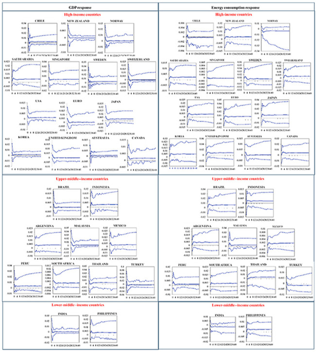
The 14 economies in this study are classified as HI countries. There are seven major trading partners in HI countries: USA, the European Union, Japan, Korea, the United Kingdom, Australia, and Canada. Fig. 1 and Fig. 2 display the economic and energy GIRFs related to a positive shock to economic variable in China and its spillover effects on the major trading partners in HI countries, respectively. Generally speaking, the spillover effects is positive for major trading partners in the HI countries. The GIRFs curve presents a positive dynamic response, and the response is not constant. The following is a detailed description.
Fig. 1.

Economic GIRFs of major trading partners in HI countries after a shock to economic variable in China (A Positive One-Standard Error Shock).
Fig. 2.

Energy GIRFs of major trading partners in HI countries after a shock to economic variable in China (A Positive One-Standard Error Shock).
USA, the European Union, and Japan, as China’s top three trading partners. First, with respect to immediate GDP response to the spillover effects of economic growth in China, USA, the European Union, and Japan responded to the positive shock of the GDP in China by 0.32%, 0.53%, and 0.66% in quarter 0, respectively. In addition, the energy consumption responded to 0.07%, 0.15%, and 0.28%, respectively. Among them, Japan’s immediate response was the highest. Subsequently, we found that the response value of GDP is decreasing but the response value of energy consumption is increasing after quarter 0. Second, for the long-term response to the spillover effects of economic growth in China. Specific to the GDP response of each country, the response value of USA (0.12%) is higher than European Union (0.02%) after the quarter 4. Subsequently, the positive response of GDP in Japan increased to 0.27% compared to almost no fluctuation in USA and European Union in the quarter 8. Furthermore, specific to the energy response of each country, the response values of various countries increased first and then decreased, and stabilized after quarter 8. The response values in USA, the European Union, and Japan are 0.41%, 0.75%, and 0.72% respectively.
Considering Korea, the United Kingdom, Australia, and Canada, they were China’s fourth to seventh largest trading partners in 2014. The largest immediate GDP response of spillover effects is 0.57% in South Korea, and the smallest is 0.19% in Australia. However, the immediate energy response of spillover effects in other countries are negligible except Australia (0.24%). For the long-term GDP response to the spillover effects, the response value of Korea stabilized at around 0.16% and 0.48% eventually. Virtually, the UK has the largest drop, the value has dropped from 0.35% to almost 0%. In other words, this positive response appears to be insignificant four quarters after the shock. On the contrary, Canada has the smallest drop, with the response value falling from 0.28% to 015%. For the long-term energy response to the spillover effects, the response values of South Korea, the United Kingdom and Canada are approximately stable at 0.47%, 0.85%, and 0.42%, respectively. However, Australia’s response value is quite insignificant.
4.1.2. Non-major trading partners in HI countries
In current study, non-major trading partners in HI countries include Chile, New Zealand, Norway, Saudi Arabia, Singapore, Sweden and Switzerland. Fig. 3 and Fig. 4 displays the economic and energy GIRFs related to a positive shock to economic variable in China and its spillover effects on the non-major trading partners in HI countries, respectively. Overall, the positive shock of GDP in China has a positive spillover effect on most non-major trading partner in the HI countries. Furthermore, all countries stabilized after fluctuations under the spillover effect.
Fig. 3.

Economic GIRFs of non-major trading partners in HI countries after a shock to economic variable in China (A Positive One-Standard Error Shock).
Fig. 4.

Energy GIRFs of non-major trading partners in HI countries after a shock to economic variable in China (A Positive One-Standard Error Shock).
Specifically, for immediate GDP response to the spillover effects of economic growth in China, it is significantly worthy to notice that the response value of Saudi Arabia is 0.14% and showed an increase trend before the quarter 2. In contrast, the immediate responses of Chile, New Zealand, Norway, Singapore, Sweden, and Switzerland all showed a decrease trend. The immediate response of their spillover effect is: Chile 0.94%, Sweden 0.83%, Singapore 0.79%, Norway 0.67%, Switzerland 0.55%, New Zealand 0.2%. For immediate energy response to the spillover effects of economic growth in China, the immediate response values of Norway and Sweden were −0.26% and 0.78%, respectively. The immediate responses of other countries were not significant.
For the long-term GDP response to the spillover effects of economic growth in China, Saudi Arabia’s positive response reached a peak of 0.5% in quarter 2, and the long-term response stabilized at 0.37% after the quarter 12. With respect to Chile, New Zealand, Norway, Singapore, Sweden, and Switzerland, the long-term GDP response value of the spillover effects began to decrease after quarter 0. Specifically, the response values of New Zealand, Norway, and Switzerland are almost close to zero after the quarter 4. That is to say, the long-term GDP response to the spillover effects of economic growth in China to New Zealand, Norway, and Switzerland almost negligible. This is in sharp contrast with the long-term GDP response of major trading partners in HI countries. In addition, the long-term GDP responses of Chile, Singapore, and Sweden remained at 0.23%, 0.33%, and 0.29%, respectively. For the long-term energy response to the spillover effects of economic growth in China, New Zealand, Saudi Arabia, Sweden, and Switzerland have all received the positive spillover effects of China’s economic growth, with long-term response values of approximately 0.29%, 0.22%, 0.59%, and 0.33%, respectively. However, Chile, Norway and Singapore have negative long-term response values of −0.02%, −0.33%, and −0.01%, respectively.
4.2. Spillover effects of economic growth in China to UMI countries
4.2.1. Major trading partners in UMI countries
UMI countries include a total of 9 countries in this study (Argentina, Brazil, Indonesia, Malaysia, Mexico, Peru, South Africa, Thailand, Turkey). Among them, the main trading partners in UMI countries include Brazil and Indonesia. The dynamic response curves to the positive shock of the Chinese economy of major trading partners in UMI countries are shown in Fig. 5 and Fig. 6 . In general, the spillover effects of economic growth in China in the two countries are heterogeneous. Next, we analyze the immediate and long-term responses of major trading partners in UMI countries.
Fig. 5.

Economic GIRFs of major trading partners in UMI countries after a shock to economic variable in China (A Positive One-Standard Error Shock).
Fig. 6.

Energy GIRFs of major trading partners in UMI countries after a shock to economic variable in China (A Positive One-Standard Error Shock).
First, from the perspective of immediate response, Brazil and Indonesia both present significant and statistical positive responses. In quarter 0, the response values of GDP in Brazil and Indonesia are 0.34% and 0.14% respectively. On the contrary, the immediate response value of energy is not obvious. Subsequently, in quarter 1, the positive GDP response value in Indonesia increased and reached the peak of 0.55% but decreased in Brazil during the same period. Besides, the energy response value of both countries showed an increasing trend in the quarter 0–2.
Second, from the perspective of long-term response, the GDP and energy response value of Indonesia remained at around 0.28% and 0.24% after quarter 4, respectively, which are significant and positive. However, the long-term GDP response in Brazil is not significant, only an extremely small positive response was maintained. The long-term energy response in Brazil is 0.61%.
4.2.2. Non-major trading partners in UMI countries
Fig. 7 and Fig. 8 display the GIRFs related to a positive shock to economic variable in China and its spillover effects on the non-major trading partners in UMI countries, respectively. Non-major trading partner countries in UMI countries in this study include: Argentina, Malaysia, Mexico, Peru, South Africa, Thailand, Turkey. On the whole, their GIRFs curves show a transition from volatility to stability, which indicates that the spillover effect of China economic growth is a long-term process.
Fig. 7.

Economic GIRFs of non-major trading partners in UMI countries after a shock to economic variable in China (A Positive One-Standard Error Shock).
Fig. 8.

Energy GIRFs of non-major trading partners in UMI countries after a shock to economic variable in China (A Positive One-Standard Error Shock).
In this task, we first investigate the immediate response to the spillover effects of economic growth in China. Evidence shows that the immediate GDP response of all non-major trading partners in UMI countries is significant. Precisely, the GDP response values of these countries are positive and remain between 0.26% and 1.76% in quarter 0. Subsequently, the response curve showed a downward trend. However, the immediate energy response of most countries is not significant.
Next, the long-time response to the spillover effects was investigated. The results prove that Argentina, Mexico, Peru, and Thailand still maintain significant positive GDP responses. To be specific, the response values were 0.39%, 0.27%, 0.34%, 0.32%, respectively. The GDP response values of Malaysia and South Africa were less significant, at 0.11% and 0.09%, respectively. Besides, the long-time GDP response in Turkey was −0.35%. For the long-term energy response, all countries except Turkey (0.17%) are positive and significant, with response values ranging from 0.11% to 0.44%.
4.3. Spillover effects of economic growth in China to LMI countries
4.3.1. Major trading partners in LMI countries
Two countries in LMI countries are selected as samples for this study: India and the Philippines. India is major trading partners of China in LMI countries. Fig. 9 and Fig. 10 display the GIRFs related to a positive shock to economic variable in China and its spillover effects on LMI countries, respectively. On the whole, the positive spillover effect of China’s GDP increase on India’s GDP is not significant, and even the spillover effect on energy consumption is negative. Considering the response process of India, for immediate GDP response to the spillover effects of economic growth in China, the response value of India is 0.61% in quarter 0, which is the stage where India GDP is most affected by China’s economic growth. For the immediate energy response, the response value is not significant in quarter 0. Then the response value of GDP and energy gradually decreases. On the other hand, for the long-term response to the spillover effects of economic growth in China, the long-term GDP and energy response value dropped to 0.02% and −0.22% in quarter 4 and continued within the 40 quarters. This shows that China’s economic growth has a certain restrictive effect on India’s economic and energy consumption growth due to the competitive relationship between China and India in the international trade market.
Fig. 9.

Economic GIRFs of LMI countries after a shock to economic variable in China (A Positive One-Standard Error Shock).
Fig. 10.

Energy GIRFs of LMI countries after a shock to economic variable in China (A Positive One-Standard Error Shock).
4.3.2. Non-major trading partners in LMI countries
In terms of the Philippines, it is non-major trading partners in LMI countries. Overall, Philippines presents significant and statistical positive responses to the shock of economic growth in China. In detail, the immediate GDP and energy response to the spillover effects of economic growth in China are 0.25% and 0% respectively in quarter 0. Hereafter, the GDP and energy response value of the Philippines increased to 0.53% and 0.29% respectively in quarter 1. Subsequently, the long-term GDP and energy response value decreases and finally stabilizes at 0.31% and 0.23%, respectively. Finally, this response persisted for 40 quarters.
5. Discussion
In the previous section, we observed that the economic and energy dynamic response in 24 countries and the EU area (including eight countries) to a positive shock to GDP in China by GVAR model. Specifically, the spillover effects to countries with different income levels have been analyzed. To better understand the impact of China’s economic recovery on the economies and energy of other countries after the COVID-19 epidemic, this section will give a comprehensive discussion on spillover effects of economic growth in China in two aspects: overview and heterogeneity of spillover effects of economic growth in China.
5.1. Overview of spillover effects of economic growth in China
This subsection summarizes the dynamic responses and provides a comprehensive overview of the spillover effects of China’s economic growth. The purpose is to find out the similarities of spillover effects of economic growth in China to different countries.
5.1.1. Overview of spillover effects on economic of other countries
Fig. 11 shows the GDP dynamic response curves of 24 countries and the EU area (including eight countries) after the positive shock of China’s GDP. Overall, it is obvious that curves can be divided into two sections according to the response change trend. Quarter 6 is the turning point, and the two curves around quarter 6 present completely different information. More specifically, before quarter 6, more than 80% of countries had the largest response value in quarter 0. This suggests that when China’s economy fluctuates, other countries will be subject to greater immediate impact. Subsequently, as the quarter increases, this spillover effect begins to decrease and is accompanied by small fluctuations. In other words, the positive spillover effect on China’s economic growth only plays a significant role in a limited period. After quarter 6, the long-term response of more than 85% of the countries is far lower than their immediate response. Then the long-term response remains stable at the lowest point. This implies that the spillover effect of China’s economic growth in the long-term is relatively weak. Regarding economic spillover effects, the RMB spillover effects between participating countries of the “The Belt and Road” initiative have been identified (Wei et al., 2020).
Fig. 11.

Overview of economic GIRFs of 24 countries and the EU area (including eight countries) after a shock to economic variable in China.
In short, the spillover effect of China’s economic growth on other countries is a long-term process, and it is positive for more than 90% of countries. The spillover effects of economic growth in China can be divided into two stages: the immediate response stage and the long-term response stage. The immediate response is the most significant. After quarter 6, the immediate response is transformed into a long-term response. The long-term response is much lower than the immediate response, which exists in 34 quarters.
5.1.2. Overview of spillover effects on energy of other countries
Fig. 12 shows the energy dynamic response curves of 24 countries and the EU area (including eight countries) after the positive shock of China’s GDP. Under the shock of China’s GDP, energy consumption showed similar dynamic characteristics. On the whole, the curve shows an overall trend of rise → decrease → stable. This is similar to the U.S. EPU impact on the output of other economies that increased for the first time in a few months, but declined after about two or three months (Trung, 2019). To be precise, the energy response curves of more than 90% of countries showed an upward trend in the quarter 0. Subsequently, the maximum response values of the entire process are reached approximately in quarter 2. Next, almost all countries’ response values fell in quarter 2–6. In the end, the response curve remained stable and stabilized at the relatively low position in quarter 6–40. This implies that China’s GDP growth has a positive spillover effect on energy consumption in most countries. Besides, this positive effect will reach the maximum after 2 quarters. But in the long run, China’s GDP growth will maintain a slight positive spillover to energy consumption in most countries. In previous studies, there is a spatial correlation between GDP and renewable energy consumption, but this correlation has only been confirmed in 26 EU countries. Regarding the mechanism of spillover effects, the “contagion” between neighboring countries leads to spatial dependence as the key (Chica-Olmo et al., 2020). In addition, although neighboring countries have different policy mechanisms, they often imitate each other’s economic development model and industrial structure configuration due to the synergy between countries (Bracco et al., 2018).
Fig. 12.

Overview of energy GIRFs of 24 countries and the EU area (including eight countries) after a shock to economic variable in China.
In conclusion, the spillover effect of China’s economic growth on energy consumption is positive for more than 80% of countries and the response curve presents an inverted U shape. The immediate and long-term response of China’s economic spillover effects to energy consumption are relatively small throughout the process. At the junction (approximately quarter 2) of the immediate and the long-term effect, the positive response value of the spillover effect is the largest.
5.2. Heterogeneity in spillover effects of economic growth in China
Sample countries were divided into 3 groups according to income level to perform GIRFs analysis in Section 3. We judge the spillover effects of economic growth in China based on the response value. According to the results, if the response value 0, the spillover effect is positive, otherwise it is negative. The results prove that spillover effects of economic growth in China are generally positive and long-term processes. However, does this spillover effect consistent across countries? To answer this question, we discuss the heterogeneity in spillover effects of economic growth in China across income levels in this subsection. We find out the heterogeneity of spillover effects by comparing the GIRFs curve between different income levels. Fig. 13 and Fig. 14 show the economic and energy GIRFs curves for the three income levels. The response value of each income level is the mean value of the response value of the corresponding countries.
Fig. 13.

Economic GIRFs of countries with different income levels after a shock to economic variable in China.
Fig. 14.

Energy GIRFs of countries with different income levels after a shock to economic variable in China.
5.2.1. Heterogeneity of spillover effects on economic of other countries
Overall, countries with different income levels have different response values to the economic shock in China. For immediate response of the spillover effects of economic growth in China, in quarter 0, the average response values of HI and UMI countries were 0.51% and 0.66%, respectively, and the LMI countries had the smallest average response value (0.43%). This confirms that HI and UMI countries are more immediately affected than LMI countries when economic growth in China. After about a year, evidence shows that the long-term response of the spillover effects on LMI countries gradually increases while on HI and UMI countries decrease. In quarter 30, the average response values of LMI and UMI countries were 0.16% and 0.17%, respectively, and the HI countries had the smallest response value (0.15%). These results indicate that the long-term response of spillover effects of economic growth in China to LMI and UMI countries is higher than that of HI countries.
In summary, the study found that the spillover effects of economic growth in China are heterogeneous among countries with different income levels. From the perspective of immediate response, the spillover effect is more obvious in HI and UMI countries than in LMI countries. In other words, LMI countries are less sensitive to positive shocks of economic growth in China. But from the perspective of long-term response, the spillover effects are more obvious to LMI countries than in HI and UMI countries. This shows that HI and UMI countries have passed some positive shocks to LMI countries after a period of time. This finding is not surprising. Similarly, the spillover effects of the U.S. EPU vary from country to country. Developing and emerging economies are more vulnerable than advanced economies. Nguyen Ba Trung pointed out that emerging Asian economies are more susceptible to US EPU shocks because the region has a higher share of trade with the US economy (Trung, 2019).
5.2.2. Heterogeneity of spillover effects on energy of other countries
The spillover effects of economic growth in China have obvious heterogeneity in the energy consumption of countries with different income levels. This may be related to the spreading mechanism of spillover effects. Trade is considered to be an important transmission mechanism for spillover effects. In addition, the size of the spillover effect also depends on the labor market rigidity, industrial structure and participation of the recipient country in the global value chain (Georgiadis, 2016; Kumar, 2019). These country characteristics lead to spillover effects that are often different between developed economies and non-developed economies. The order of the response value of energy consumption has been consistent in 40 quarters: HI countries (0.11%–0.45%) >UMI countries (0.08%–0.33%) >LMI countries (−0.02%-0.05%). This shows that the heterogeneity of spillover effects of economic growth in China on energy consumption is related to income levels. Specifically, the response value of energy consumption increases as income levels increase. The energy consumption of developed countries has the largest positive response value to economic growth in China.
6. Conclusion
The prevention and control policies to fight COVID-19 has triggered the global economic recession and energy challenges in 2020. Thanks to the early effective control, China has become the first major economy to recover from COVID-19. This study sought to investigates the impact of GDP growth in China on economic and energy of other countries, in order to test the spillover effects of China’s economic recovery among various countries. The empirical strategy adopted in this study was an application of a GVAR model, which can examine the international spillover effects of shocks on the basis of the interdependence between economies. Notably, 24 countries and the EU area (including eight countries) are selected and divided into three income levels to obtain a heterogeneous assessment of the spillover effects of China’s economic recovery.
First, an dynamic analysis of spillover effects overview of economic growth in China indicate that the number of countries that experience spillover effects from a Chinese economic recovery is significant. The selected countries have been affected by the positive spillover effects of the Chinese economy in terms of economy and energy. From an economic response point of view, results confirm that China’s huge economic scale will play an important role in revitalizing the global economy. Moreover, this spillover effect is continuous but not constant. Regardless of income levels, the immediate GDP response of countries to China’s spillover effects is the greatest, and then gradually declines. After about 6 quarters, it stabilizes at a certain value and turns into a continuous and weak long-term response. This long-term GDP response will last approximately 34 quarters. From an energy response point of view, China’s economic growth has a small positive effect on the energy consumption of more than 80% of countries. This driving effect continued to strengthen in the first two quarters after the shock, and then weakened. Finally, energy consumption will maintain a stable long-term positive response.
Second, results from heterogeneous assessment indicate that the spillover effects of China’s economic recovery are heterogeneous to countries with different income levels. From an economic response point of view, the heterogeneity is manifested in two aspects of spillover effects. The first aspect is the response speed. The average immediate response of HI countries (0.51%) and UMI countries (0.66%) are higher than that of LMI countries (0.43%). This shows that compared to LMI countries, HI and UMI countries are more susceptible to the positive shock of China’s economic recovery. In other words, LMI countries are slower to receive positive shocks from China than HI and UMI countries. The second aspect is the delivery channel. The average long-term response of HI countries (0.15%) and UMI countries (0.17%) is lower than that of LMI countries (0.16%). In this sense, it would suggest that the positive spillover effects of China’s economy passed slightly from HI countries and LMI countries to UMI countries in about a year. From an energy response point of view, whether it is immediate response or long-term response, the heterogeneity of the spillover effects of economic growth in China remains consistent. The response of HI countries (0.11%–0.45%) is greater than that of UMI countries (0.08%–0.33%), and the smallest is LMI countries (−0.02%–0.05%). That is to say, the level of income is consistent with the level of response value.
Our conclusions support that China will play an important role in the global economic recovery after COVID-19 epidemic. To get rid of the economic and energy crisis caused by COVID-19 epidemic, international exchanges and cooperation are essential. In particular, China’s right to speak in the field of international economy and energy utilization should be enhanced. Furthermore, decision makers at the global and national levels need to jointly respond to and manage global energy.
The GVAR model can predict economic changes in a range of countries. However, due to the availability of data, this work can only simulate empirical results from 1991 to 2014 data to speculate on China’s impact on economic growth and energy consumption in other countries after the COVID-19 epidemic. Taking into account the repetitive nature of the COVID-19 epidemic, the control measures that some governments have to continue to take after the peak period have had an impact on local economic development and energy consumption, which cannot be simulated by our model. In the future, we can consider using updated data during the COVID-19 epidemic to solve this problem.
CRediT authorship contribution statement
Qiang Wang: Conceptualization, Methodology, Software, Data curation, Writing - original draft, Supervision, Writing - review & editing. Fuyu Zhang: Methodology, Data curation, Investigation, Writing - original draft, Writing - review & editing.
Declaration of competing interest
The authors declare that they have no known competing financial interests or personal relationships that could have appeared to influence the work reported in this paper.
Acknowledgement
The authors would like to thank the editor and these anonymous reviewers for their helpful and constructive comments that greatly contributed to improving the final version of the manuscript. This work is supported by National Natural Science Foundation of China (Grant No. 71874203), Humanities and Social Science Fund of Ministry of Education of China (Grant No.18YJA790081), Natural Science Foundation of Shandong Province, China (Grant No. ZR2018MG016).
Handling editor: Dr Sandra Caeiro
Appendix A.
Table A1.
Weight Matrices (based on time-varying weights)
| Country | ARGENTINA | AUSTRALIA | BRAZIL | CANADA | CHINA | CHILE | EURO | INDIA | INDONESIA | JAPAN | KOREA | MALAYSIA | MEXICO | NORWAY | NEW ZEALAND | PERU | PHILIPPINES | SOUTH AFRICA | SAUDI ARABIA | SINGAPORE | SWEDEN | SWITZERLAND | THAILAND | TURKEY | UNITED KINGDOM | USA |
|---|---|---|---|---|---|---|---|---|---|---|---|---|---|---|---|---|---|---|---|---|---|---|---|---|---|---|
| ARGENTINA | 0 | 0.0022 | 0.0915 | 0.0026 | 0.0054 | 0.0385 | 0.0069 | 0.0043 | 0.0062 | 0.002 | 0.0025 | 0.0043 | 0.0039 | 0.0007 | 0.0025 | 0.0263 | 0.0043 | 0.0076 | 0.0028 | 0.0006 | 0.0014 | 0.0024 | 0.0048 | 0.0029 | 0.0016 | 0.0047 |
| AUSTRALIA | 0.0083 | 0 | 0.0046 | 0.004 | 0.0481 | 0.0105 | 0.014 | 0.0301 | 0.0323 | 0.057 | 0.0398 | 0.0424 | 0.0024 | 0.0023 | 0.1956 | 0.0038 | 0.0175 | 0.0161 | 0.0059 | 0.0362 | 0.0085 | 0.0076 | 0.0434 | 0.0062 | 0.0117 | 0.0118 |
| BRAZIL | 0.3023 | 0.0035 | 0 | 0.0069 | 0.0336 | 0.0727 | 0.0282 | 0.0241 | 0.012 | 0.0136 | 0.0194 | 0.0082 | 0.0135 | 0.0114 | 0.0032 | 0.0559 | 0.0034 | 0.0172 | 0.0139 | 0.0068 | 0.0085 | 0.0089 | 0.0121 | 0.012 | 0.009 | 0.0231 |
| CANADA | 0.0209 | 0.0083 | 0.0157 | 0 | 0.0199 | 0.0196 | 0.0173 | 0.0114 | 0.0086 | 0.0175 | 0.013 | 0.0051 | 0.0287 | 0.0159 | 0.0137 | 0.0525 | 0.0093 | 0.0076 | 0.0136 | 0.0043 | 0.0067 | 0.0119 | 0.0069 | 0.01 | 0.0247 | 0.1994 |
| CHINA | 0.1412 | 0.3063 | 0.2185 | 0.0834 | 0 | 0.2549 | 0.1562 | 0.15 | 0.1616 | 0.2638 | 0.2901 | 0.1761 | 0.0969 | 0.0545 | 0.2135 | 0.2186 | 0.1548 | 0.1934 | 0.1698 | 0.1581 | 0.0574 | 0.0618 | 0.1796 | 0.1255 | 0.0845 | 0.1779 |
| CHILE | 0.0436 | 0.0033 | 0.0246 | 0.003 | 0.013 | 0 | 0.0071 | 0.0079 | 0.0013 | 0.0086 | 0.009 | 0.0012 | 0.005 | 0.0014 | 0.0025 | 0.0465 | 0.0009 | 0.0017 | 0.0005 | 0.0003 | 0.0026 | 0.0021 | 0.0027 | 0.0029 | 0.0023 | 0.0086 |
| EURO | 0.1584 | 0.0892 | 0.209 | 0.0611 | 0.1554 | 0.1412 | 0 | 0.164 | 0.0778 | 0.0942 | 0.0845 | 0.0953 | 0.0698 | 0.453 | 0.1044 | 0.1415 | 0.1056 | 0.2571 | 0.1317 | 0.0999 | 0.5389 | 0.5211 | 0.084 | 0.4642 | 0.4953 | 0.1428 |
| INDIA | 0.0182 | 0.0295 | 0.0293 | 0.0064 | 0.026 | 0.024 | 0.0263 | 0 | 0.0533 | 0.0134 | 0.0233 | 0.0383 | 0.0091 | 0.004 | 0.0142 | 0.0171 | 0.0113 | 0.0625 | 0.1003 | 0.0371 | 0.0095 | 0.04 | 0.0247 | 0.033 | 0.0179 | 0.0203 |
| INDONESIA | 0.0161 | 0.0256 | 0.0105 | 0.0036 | 0.0255 | 0.0032 | 0.0098 | 0.0439 | 0 | 0.0386 | 0.0333 | 0.0535 | 0.002 | 0.0016 | 0.0217 | 0.0043 | 0.0377 | 0.0104 | 0.0146 | 0.1053 | 0.0027 | 0.002 | 0.0522 | 0.0102 | 0.0031 | 0.0086 |
| JAPAN | 0.0224 | 0.1513 | 0.0401 | 0.0276 | 0.1223 | 0.0772 | 0.0407 | 0.0379 | 0.1485 | 0 | 0.1212 | 0.125 | 0.0285 | 0.017 | 0.0765 | 0.0482 | 0.1753 | 0.07 | 0.1434 | 0.0684 | 0.016 | 0.0248 | 0.182 | 0.0178 | 0.0196 | 0.0651 |
| KOREA | 0.0182 | 0.0695 | 0.0376 | 0.0121 | 0.1051 | 0.0532 | 0.0246 | 0.0383 | 0.0772 | 0.0776 | 0 | 0.0495 | 0.0219 | 0.025 | 0.0451 | 0.0426 | 0.0787 | 0.0253 | 0.1067 | 0.0707 | 0.0086 | 0.0082 | 0.0379 | 0.0325 | 0.0136 | 0.0335 |
| MALAYSIA | 0.0127 | 0.0363 | 0.01 | 0.0035 | 0.0388 | 0.0034 | 0.0121 | 0.0319 | 0.0726 | 0.0386 | 0.0239 | 0 | 0.0083 | 0.0034 | 0.0357 | 0.0029 | 0.0392 | 0.0143 | 0.0098 | 0.1572 | 0.0041 | 0.0045 | 0.0728 | 0.0069 | 0.0081 | 0.0128 |
| MEXICO | 0.0266 | 0.0062 | 0.0272 | 0.0369 | 0.0153 | 0.0292 | 0.0183 | 0.0128 | 0.0037 | 0.0122 | 0.0161 | 0.0051 | 0 | 0.0016 | 0.0067 | 0.0348 | 0.0038 | 0.0075 | 0.0031 | 0.0059 | 0.0037 | 0.0073 | 0.0071 | 0.0056 | 0.0041 | 0.1602 |
| NORWAY | 0.0013 | 0.0013 | 0.0049 | 0.0056 | 0.0025 | 0.0012 | 0.0347 | 0.0023 | 0.001 | 0.0029 | 0.0068 | 0.0016 | 0.0003 | 0 | 0.001 | 0.0027 | 0.0007 | 0.0025 | 0.0003 | 0.0038 | 0.1264 | 0.0032 | 0.0021 | 0.0069 | 0.0384 | 0.0031 |
| NEW ZEALAND | 0.0014 | 0.0349 | 0.0005 | 0.0011 | 0.0047 | 0.0012 | 0.0023 | 0.0021 | 0.004 | 0.0042 | 0.0038 | 0.0063 | 0.0006 | 0.0004 | 0 | 0.002 | 0.0055 | 0.0021 | 0.0022 | 0.005 | 0.001 | 0.0007 | 0.0051 | 0.0007 | 0.0026 | 0.0023 |
| PERU | 0.0147 | 0.0005 | 0.0103 | 0.0045 | 0.0055 | 0.0273 | 0.0038 | 0.0027 | 0.0008 | 0.0028 | 0.004 | 0.0004 | 0.0033 | 0.0018 | 0.0022 | 0 | 0.0006 | 0.0005 | 0.0002 | 0.0001 | 0.0018 | 0.005 | 0.0019 | 0.0017 | 0.0007 | 0.0053 |
| PHILIPPINES | 0.0048 | 0.0055 | 0.003 | 0.0019 | 0.0153 | 0.0014 | 0.0045 | 0.0038 | 0.0146 | 0.0167 | 0.0159 | 0.0139 | 0.0025 | 0.0006 | 0.0107 | 0.002 | 0 | 0.0017 | 0.0072 | 0.021 | 0.001 | 0.0016 | 0.0225 | 0.0014 | 0.0013 | 0.0057 |
| SOUTH AFRICA | 0.0089 | 0.0052 | 0.0065 | 0.0015 | 0.0238 | 0.0017 | 0.0147 | 0.0272 | 0.0065 | 0.0082 | 0.0051 | 0.005 | 0 | 0.0025 | 0.0047 | 0.0019 | 0.0022 | 0 | 0.0197 | 0.0038 | 0.0057 | 0.0056 | 0.0125 | 0.0086 | 0.0123 | 0.0049 |
| SAUDI ARABIA | 0.0084 | 0.0055 | 0.0168 | 0.0044 | 0.0276 | 0.0017 | 0.0246 | 0.0979 | 0.0255 | 0.0486 | 0.0599 | 0.0102 | 0.0013 | 0.0006 | 0.0189 | 0.0016 | 0.0342 | 0.0636 | 0 | 0.0282 | 0.0075 | 0.0095 | 0.0313 | 0.0257 | 0.0085 | 0.0221 |
| SINGAPORE | 0.0024 | 0.0482 | 0.01 | 0.0026 | 0.0287 | 0.0012 | 0.0168 | 0.0434 | 0.1358 | 0.0248 | 0.0428 | 0.1643 | 0.0028 | 0.0104 | 0.0364 | 0.0011 | 0.0903 | 0.0195 | 0.042 | 0 | 0.0044 | 0.0217 | 0.0532 | 0.0032 | 0.0109 | 0.0152 |
| SWEDEN | 0.0033 | 0.006 | 0.0066 | 0.0027 | 0.0053 | 0.0052 | 0.052 | 0.0054 | 0.0035 | 0.0032 | 0.0032 | 0.0029 | 0.0019 | 0.1021 | 0.0047 | 0.0057 | 0.0024 | 0.0116 | 0.0042 | 0.0024 | 0 | 0.0075 | 0.0042 | 0.0154 | 0.0248 | 0.0046 |
| SWITZERLAND | 0.0087 | 0.0085 | 0.0139 | 0.0059 | 0.0166 | 0.0099 | 0.0909 | 0.058 | 0.0023 | 0.0093 | 0.0041 | 0.0061 | 0.004 | 0.0095 | 0.0049 | 0.0298 | 0.0063 | 0.0205 | 0.0094 | 0.0104 | 0.0127 | 0 | 0.0281 | 0.0394 | 0.0628 | 0.0168 |
| THAILAND | 0.0148 | 0.0371 | 0.0118 | 0.0039 | 0.0273 | 0.0079 | 0.0107 | 0.02 | 0.0537 | 0.0496 | 0.017 | 0.0693 | 0.0065 | 0.004 | 0.0291 | 0.011 | 0.0583 | 0.0242 | 0.0263 | 0.0432 | 0.0056 | 0.0127 | 0 | 0.007 | 0.0075 | 0.012 |
| TURKEY | 0.0064 | 0.0031 | 0.006 | 0.0026 | 0.0083 | 0.0048 | 0.0429 | 0.0121 | 0.0075 | 0.0024 | 0.0081 | 0.0029 | 0.0012 | 0.0089 | 0.003 | 0.0054 | 0.0016 | 0.0089 | 0.0146 | 0.0019 | 0.0136 | 0.0162 | 0.004 | 0 | 0.0173 | 0.0059 |
| UNITED KINGDOM | 0.0131 | 0.026 | 0.0211 | 0.0273 | 0.0274 | 0.0135 | 0.1763 | 0.0331 | 0.0089 | 0.0155 | 0.0153 | 0.0128 | 0.0062 | 0.2092 | 0.0341 | 0.0109 | 0.0089 | 0.0506 | 0.0146 | 0.0207 | 0.0909 | 0.1104 | 0.0193 | 0.0708 | 0 | 0.0333 |
| USA | 0.1229 | 0.0869 | 0.1702 | 0.6846 | 0.1986 | 0.1954 | 0.1644 | 0.1355 | 0.0811 | 0.175 | 0.1378 | 0.1001 | 0.6794 | 0.0582 | 0.115 | 0.2309 | 0.1473 | 0.1034 | 0.1431 | 0.1087 | 0.0608 | 0.1033 | 0.1056 | 0.0895 | 0.1174 | 0 |
Table A.2.
ADF-WS Unit Root Tests for the Domestic Variables at the 5% Significance Level (based on AIC order selection)
| Domestic Variables |
gdp |
ens |
enc |
ce |
ep |
|||||
|---|---|---|---|---|---|---|---|---|---|---|
| Statistic | ADF | WS | ADF | WS | ADF | WS | ADF | WS | ADF | WS |
| Critical Value | −3.4500 | −3.2400 | −3.4500 | −3.2400 | −3.4500 | −3.2400 | −3.4500 | −3.2400 | −3.4500 | −3.2400 |
| ARGENTINA | −4.1797 | −3.9375 | −3.8982 | −4.1010 | −3.4940 | −3.1467 | −3.1460 | −3.2677 | −6.4350 | −6.3658 |
| AUSTRALIA | −4.7801 | −3.4944 | −4.4928 | −4.0676 | −4.1932 | −3.8488 | −3.1847 | −3.3379 | −6.8741 | −7.0621 |
| BRAZIL | −6.2461 | −6.1095 | −2.7654 | −3.0185 | −3.3978 | −3.6190 | −3.4471 | −3.4761 | −6.0956 | −6.2826 |
| CANADA | −5.2171 | −5.2781 | −4.4161 | −4.6086 | −4.5132 | −4.7406 | −2.5923 | −2.8845 | −6.7998 | −6.9568 |
| CHINA | −3.0725 | −3.2820 | −1.5861 | −1.8980 | −1.6320 | −1.9566 | −2.8482 | −2.9930 | −7.0223 | −7.2506 |
| CHILE | −5.3801 | −5.3176 | −3.2828 | −3.2238 | −3.4836 | −3.4270 | −1.8647 | −2.1866 | −6.6226 | −6.7690 |
| EURO | −4.6047 | −4.7984 | −3.3836 | −3.6408 | −3.1953 | −3.4067 | −2.8916 | −2.5394 | −6.7511 | −6.8388 |
| INDIA | −3.5131 | −3.8511 | −2.5888 | −2.8501 | −3.3319 | −3.3029 | −3.8343 | −3.9823 | −7.9571 | −5.6312 |
| INDONESIA | −5.1936 | −5.3728 | −4.1345 | −4.2235 | −2.2468 | −2.4889 | −3.8543 | −4.0278 | −7.0809 | −7.3076 |
| JAPAN | −5.9627 | −6.2116 | −4.7642 | −4.4749 | −4.4883 | −4.6786 | −3.8458 | −4.0166 | −4.1726 | −4.3832 |
| KOREA | −5.9783 | −6.1907 | −3.3352 | −3.4010 | −4.0557 | −3.9761 | −4.0218 | −4.2549 | −7.1862 | −7.3727 |
| MALAYSIA | −5.4809 | −5.5928 | −3.5569 | −3.7982 | −4.7622 | −4.9925 | −3.6614 | −3.8089 | −5.7194 | −5.9025 |
| MEXICO | −5.8543 | −5.9420 | −3.7191 | −3.7746 | −3.1301 | −3.3800 | −3.6907 | −3.8512 | −5.0878 | −5.2730 |
| NORWAY | −7.5500 | −7.6177 | −4.3368 | −4.4266 | −4.5818 | −4.7518 | −3.7505 | −3.8511 | −6.7569 | −6.8283 |
| NEW ZEALAND | −5.4540 | −5.2640 | −4.4403 | −3.4215 | −2.0556 | −2.0680 | −3.6408 | −3.8995 | −6.2689 | −6.4390 |
| PERU | −4.6514 | −4.8855 | −4.1689 | −4.2793 | −3.8519 | −3.0645 | −3.9081 | −4.0507 | −6.9377 | −4.6261 |
| PHILIPPINES | −7.0875 | −7.2218 | −3.2873 | −3.5254 | −4.3177 | −1.1273 | −4.0216 | −3.6933 | −5.0553 | −5.0944 |
| SOUTH AFRICA | −4.4294 | −4.4513 | −2.7299 | −2.2895 | −3.9212 | −4.1249 | −4.3080 | −3.4486 | −6.2834 | −6.4625 |
| SAUDI ARABIA | −3.3000 | −3.3831 | −4.1405 | −4.1834 | −4.0707 | −4.1356 | −3.3657 | −3.5530 | −5.4551 | −5.1991 |
| SINGAPORE | −5.6706 | −5.8964 | −4.1226 | −4.2293 | −3.7536 | −3.9922 | −4.0149 | −4.2306 | −4.9196 | −5.0807 |
| SWEDEN | −5.1587 | −5.1827 | −4.2722 | −4.5003 | −4.7655 | −5.0035 | −4.0547 | −4.2503 | −6.7961 | −6.9616 |
| SWITZERLAND | −4.2152 | −4.4154 | −4.1320 | −4.0658 | −3.9080 | −4.1525 | −3.4733 | −3.8132 | −4.5292 | −4.7384 |
| THAILAND | −6.0665 | −6.2239 | −3.9638 | −3.5629 | −3.1085 | −3.3459 | −2.8523 | −3.1145 | −6.2907 | −6.4859 |
| TURKEY | −6.2611 | −6.4712 | −3.1743 | −3.5151 | −3.8844 | −4.0995 | −3.9522 | −4.1833 | −7.4103 | −7.5694 |
| UNITED KINGDOM | −4.6446 | −4.4374 | −5.0820 | −2.1948 | −3.5878 | −3.6590 | −3.1473 | −3.3701 | −7.9851 | −8.0395 |
| USA | −4.4470 | −4.5581 | −5.5546 | −5.5843 | −4.3927 | −4.6139 | −4.1695 | −4.4049 | −6.7147 | −6.9032 |
Note: The ADF-WS statistics for all variables are based on regressions with trend.
Table A.3.
ADF-WS Unit Root Tests for the Foreign Variables at the 5% Significance Level
| Foreign Variables | gdps | enss | encs | ces | eps | |||||
|---|---|---|---|---|---|---|---|---|---|---|
| Statistic | ADF | WS | ADF | WS | ADF | WS | ADF | WS | ADF | WS |
| Critical Value | −3.4500 | −3.2400 | −3.4500 | −3.2400 | −3.4500 | −3.2400 | −3.4500 | −3.2400 | −3.4500 | −3.2400 |
| ARGENTINA | −6.3360 | −6.5041 | −5.3356 | −5.4215 | −3.6922 | −3.9498 | −4.1462 | −4.1480 | −6.3733 | −6.5586 |
| AUSTRALIA | −5.3046 | −5.4680 | −3.4233 | −3.6429 | −3.7878 | −4.0285 | −3.7600 | −4.0539 | −6.2779 | −6.4340 |
| BRAZIL | −5.0676 | −5.2434 | −7.0332 | −7.2008 | −3.6447 | −3.9043 | −3.5050 | −3.7441 | −6.7412 | −6.9219 |
| CANADA | −4.6879 | −4.8096 | −5.6125 | −5.6525 | −4.4928 | −4.7133 | −4.6947 | −4.9049 | −7.2526 | −7.4049 |
| CHINA | −5.4082 | −5.5778 | −3.9894 | −4.2251 | −4.3677 | −4.5955 | −4.6345 | −4.8793 | −6.7250 | −6.8951 |
| CHILE | −5.5918 | −5.7715 | −4.4215 | −4.4685 | −3.7346 | −3.9857 | −3.9278 | −4.1096 | −6.2919 | −6.4745 |
| EURO | −5.2221 | −5.2955 | −5.0760 | −2.8812 | −3.4125 | −3.6634 | −3.8008 | −4.0776 | −7.2824 | −7.3943 |
| INDIA | −5.1594 | −5.3223 | −4.6555 | −4.4982 | −3.6236 | −3.8321 | −3.8690 | −4.1312 | −6.6689 | −6.8048 |
| INDONESIA | −5.6030 | −5.8538 | −3.6064 | −3.6805 | −3.7277 | −3.9636 | −3.8867 | −4.1212 | −4.5273 | −4.7284 |
| JAPAN | −5.2453 | −5.4021 | −5.1273 | −5.1770 | −3.5165 | −3.7751 | −4.1027 | −4.3439 | −6.0109 | −6.1897 |
| KOREA | −5.1240 | −5.2773 | −4.0363 | −4.2474 | −3.2799 | −3.5056 | −3.9432 | −4.2189 | −6.1728 | −6.3462 |
| MALAYSIA | −5.5054 | −5.7534 | −4.1624 | −4.1481 | −3.5761 | −3.8277 | −4.0552 | −4.2696 | −6.1520 | −6.3293 |
| MEXICO | −4.7573 | −4.8863 | −5.5875 | −5.6382 | −4.5555 | −4.7772 | −4.7379 | −4.9500 | −6.8079 | −6.9689 |
| NORWAY | −4.4700 | −4.6017 | −4.2447 | −2.1782 | −3.5644 | −3.7682 | −3.5879 | −3.5648 | −7.1622 | −7.2667 |
| NEW ZEALAND | −5.4361 | −5.4938 | −3.3535 | −3.5870 | −3.8352 | −3.9837 | −3.2730 | −3.5811 | −6.5952 | −6.7766 |
| PERU | −5.8831 | −6.0559 | −5.7195 | −5.6267 | −3.9398 | −4.1898 | −3.8138 | −3.9909 | −6.4752 | −6.6555 |
| PHILIPPINES | −5.5083 | −5.7576 | −3.9365 | −4.1540 | −4.0123 | −4.2440 | −4.0574 | −4.3129 | −6.4021 | −6.5803 |
| SOUTH AFRICA | −5.1146 | −5.2690 | −4.1997 | −2.6005 | −3.6932 | −3.8661 | −3.3086 | −3.3706 | −4.8730 | −5.0944 |
| SAUDI ARABIA | −5.5877 | −5.7445 | −3.7688 | −3.7094 | −4.1357 | −4.3728 | −4.2114 | −4.4703 | −6.4678 | −6.5988 |
| SINGAPORE | −5.2675 | −5.4465 | −3.6236 | −3.8587 | −4.0947 | −4.3533 | −3.5962 | −3.8240 | −5.8860 | −6.0583 |
| SWEDEN | −4.7368 | −4.9849 | −3.8001 | −2.7104 | −3.5201 | −3.7569 | −3.2276 | −2.9517 | −7.0180 | −7.1048 |
| SWITZERLAND | −4.4910 | −4.6569 | −3.4680 | −3.1821 | −3.7493 | −3.9349 | −3.3265 | −3.0560 | −6.9460 | −7.0341 |
| THAILAND | −5.4017 | −5.5743 | −4.0665 | −4.3151 | −3.8032 | −4.0517 | −4.2544 | −4.5080 | −6.4768 | −6.6343 |
| TURKEY | −4.9811 | −5.1506 | −3.8650 | −3.9738 | −3.6941 | −3.9077 | −3.1269 | −3.1338 | −6.8586 | −6.9685 |
| UNITED KINGDOM | −4.7779 | −4.9388 | −3.2766 | −3.5259 | −3.6283 | −3.8592 | −3.2154 | −3.0011 | −6.7794 | −6.8756 |
| USA | −5.4208 | −5.5869 | −3.1704 | −3.4313 | −3.5972 | −3.8589 | −3.9596 | −4.2090 | −6.9715 | −7.1560 |
Note: The ADF-WS statistics for all variables are based on regressions with trend.
Table A.4.
ADF-WS Unit Root Tests for the Global Variables at the 5% Significance Level
| Global Variables | poil (with trend) | Dpoil | ||
|---|---|---|---|---|
| Test | ADF | WS | ADF | WS |
| Critical Value | −3.4500 | −3.2400 | −2.8900 | −2.5500 |
| Statistic | −2.8492 | −2.5689 | −7.2978 | −7.4784 |
Note: The ADF-WS statistics for all variables are based on regressions with trend.
Table A.5.
Cointegrating Relationships for the Individual VARX∗ Models
| Country | Cointegrating relations | Country | Cointegrating relations |
|---|---|---|---|
| ARGENTINA | 2 | NORWAY | 2 |
| AUSTRALIA | 4 | NEW ZEALAND | 3 |
| BRAZIL | 2 | PERU | 4 |
| CANADA | 4 | PHILIPPINES | 2 |
| CHINA | 2 | SOUTH AFRICA | 2 |
| CHILE | 3 | SAUDI ARABIA | 2 |
| EURO | 3 | SINGAPORE | 2 |
| INDIA | 2 | SWEDEN | 3 |
| INDONESIA | 2 | SWITZERLAND | 3 |
| JAPAN | 3 | THAILAND | 2 |
| KOREA | 3 | TURKEY | 1 |
| MALAYSIA | 3 | UNITED KINGDOM | 3 |
| MEXICO | 1 | USA | 3 |
Table A.6.
F-Statistics for the Serial Correlation Test of the VECMX∗ Residuals
| Fcrit_0.05 | gdp | ens | enc | ce | ep | poil | ||
|---|---|---|---|---|---|---|---|---|
| ARGENTINA | F(1,84) | 3.9546 | 0.1928 | 5.0225 | 5.3303 | 6.6199 | 1.4987 | 3.9565 |
| AUSTRALIA | F(1,82) | 3.9574 | 0.0214 | 4.3683 | 0.5661 | 7.6872 | 0.5027 | 0.0628 |
| BRAZIL | F(1,84) | 3.9546 | 3.5408 | 10.3475 | 2.6663 | 8.5949 | 0.0001 | 2.4675 |
| CANADA | F(1,82) | 3.9574 | 0.4484 | 7.4472 | 2.9761 | 6.6478 | 1.6210 | 0.0181 |
| CHINA | F(1,84) | 3.9546 | 3.8779 | 5.1653 | 4.5701 | 3.9169 | 0.4684 | 6.4438 |
| CHILE | F(1,83) | 3.9560 | 0.4384 | 5.5140 | 5.7307 | 7.0436 | 0.0000 | 0.0056 |
| EURO | F(1,83) | 3.9560 | 3.9680 | 10.5857 | 4.4479 | 4.2891 | 0.6341 | 0.1598 |
| INDIA | F(1,84) | 3.9546 | 5.4772 | 7.2955 | 9.2493 | 5.1969 | 0.5311 | 8.5467 |
| INDONESIA | F(1,84) | 3.9546 | 7.6180 | 12.5809 | 8.1032 | 7.4524 | 6.6773 | 0.2706 |
| JAPAN | F(1,83) | 3.9560 | 0.1992 | 6.5652 | 4.5381 | 3.7402 | 0.0840 | 0.0023 |
| KOREA | F(1,83) | 3.9560 | 2.4615 | 3.3333 | 4.6204 | 6.9476 | 1.1210 | 1.0996 |
| MALAYSIA | F(1,83) | 3.9560 | 0.9438 | 8.6651 | 7.1090 | 6.9810 | 0.2195 | 1.3564 |
| MEXICO | F(1,85) | 3.9532 | 16.1603 | 7.8246 | 7.3087 | 8.8056 | 12.0362 | 11.7499 |
| NORWAY | F(1,84) | 3.9546 | 1.2755 | 6.4783 | 7.0858 | 8.4051 | 0.0007 | 2.9191 |
| NEW ZEALAND | F(1,83) | 3.9560 | 0.0255 | 4.4963 | 7.4543 | 4.7486 | 0.9389 | 0.1070 |
| PERU | F(1,82) | 3.9574 | 0.2388 | 3.2716 | 2.4823 | 5.7063 | 6.6124 | 0.4523 |
| PHILIPPINES | F(1,84) | 3.9546 | 0.2401 | 3.2801 | 2.1452 | 5.6706 | 1.5776 | 1.7384 |
| SOUTH AFRICA | F(1,84) | 3.9546 | 0.1442 | 3.9402 | 4.6563 | 3.0450 | 0.0788 | 0.7951 |
| SAUDI ARABIA | F(1,84) | 3.9546 | 0.4766 | 5.3393 | 6.9231 | 4.8987 | 0.3416 | 0.0511 |
| SINGAPORE | F(1,84) | 3.9546 | 6.9714 | 8.6024 | 8.9919 | 3.7678 | 0.7462 | 3.3654 |
| SWEDEN | F(1,83) | 3.9560 | 3.4615 | 6.7646 | 1.7038 | 5.9908 | 0.0480 | 0.0595 |
| SWITZERLAND | F(1,83) | 3.9560 | 4.6091 | 6.5031 | 4.5529 | 6.1763 | 0.2862 | 0.1542 |
| THAILAND | F(1,84) | 3.9546 | 3.0088 | 3.9887 | 10.7735 | 8.4398 | 1.2937 | 0.0242 |
| TURKEY | F(1,85) | 3.9532 | 0.1992 | 7.0600 | 8.0741 | 8.2393 | 9.3135 | 5.8668 |
| UNITED KINGDOM | F(1,83) | 3.9560 | 5.9550 | 0.7812 | 0.4718 | 2.3444 | 0.0443 | 0.4752 |
| USA | F(1,83) | 3.9560 | 0.0898 | 1.3010 | 6.3926 | 4.4923 | 1.2952 | 0.1783 |
Table A.7.
Test for Weak Exogeneity at the 5% Significance Level
| Country | F test | Fcrit_0.05 | gdps | enss | encs | ces | eps |
|---|---|---|---|---|---|---|---|
| ARGENTINA | F(2,70) | 3.1277 | 2.7813 | 3.1526 | 0.2548 | 0.8281 | 0.3581 |
| AUSTRALIA | F(4,75) | 2.4937 | 1.7827 | 0.4290 | 0.4920 | 0.5750 | 1.1216 |
| BRAZIL | F(2,77) | 3.1154 | 2.8509 | 0.3171 | 0.0045 | 0.4549 | 1.0433 |
| CANADA | F(4,75) | 2.4937 | 1.4242 | 1.1611 | 0.6037 | 0.4728 | 3.5204 |
| CHINA | F(2,77) | 3.1154 | 0.7033 | 2.3784 | 0.3121 | 2.7339 | 0.2126 |
| CHILE | F(3,76) | 2.7249 | 2.6360 | 0.0222 | 0.2771 | 0.2056 | 1.7694 |
| EURO | F(3,76) | 2.7249 | 1.9957 | 0.8963 | 1.8108 | 1.9825 | 2.5645 |
| INDIA | F(2,77) | 3.1154 | 0.2430 | 0.5906 | 0.6448 | 0.2050 | 1.6554 |
| INDONESIA | F(2,77) | 3.1154 | 1.5168 | 0.2737 | 0.8053 | 0.1005 | 0.4182 |
| JAPAN | F(3,76) | 2.7249 | 0.6049 | 0.3049 | 0.2909 | 0.1584 | 1.8717 |
| KOREA | F(3,76) | 2.7249 | 0.0870 | 0.3642 | 0.7023 | 0.2665 | 0.4363 |
| MALAYSIA | F(3,76) | 2.7249 | 1.7340 | 0.1627 | 0.9371 | 1.4577 | 2.7364 |
| MEXICO | F(1,78) | 3.9635 | 3.1262 | 0.9507 | 0.0856 | 0.0699 | 0.1414 |
| NORWAY | F(2,77) | 3.1154 | 0.4327 | 0.5086 | 1.4988 | 2.4832 | 0.6608 |
| NEW ZEALAND | F(3,76) | 2.7249 | 1.8369 | 0.5617 | 0.2242 | 0.0386 | 2.8446 |
| PERU | F(4,75) | 2.4937 | 3.3553 | 0.9076 | 0.6788 | 1.0199 | 5.0377 |
| PHILIPPINES | F(2,77) | 3.1154 | 0.5462 | 0.1395 | 0.7239 | 0.3860 | 0.4056 |
| SOUTH AFRICA | F(2,77) | 3.1154 | 3.7838 | 0.2428 | 0.0153 | 0.0922 | 1.6493 |
| SAUDI ARABIA | F(2,77) | 3.1154 | 2.5254 | 0.2852 | 0.1440 | 0.0698 | 5.3009 |
| SINGAPORE | F(2,77) | 3.1154 | 0.0839 | 0.1929 | 0.0735 | 0.6244 | 0.2641 |
| SWEDEN | F(3,76) | 2.7249 | 2.8824 | 1.8380 | 0.0831 | 0.3917 | 1.0388 |
| SWITZERLAND | F(3,76) | 2.7249 | 1.8246 | 0.4850 | 0.0740 | 0.0421 | 1.1802 |
| THAILAND | F(2,77) | 3.1154 | 3.7144 | 0.0861 | 0.2581 | 0.2840 | 1.5262 |
| TURKEY | F(1,78) | 3.9635 | 1.0656 | 0.0997 | 0.6951 | 0.3560 | 0.6540 |
| UNITED KINGDOM | F(3,76) | 2.7249 | 3.9173 | 0.8811 | 1.1482 | 1.1481 | 1.1808 |
| USA | F(3,76) | 2.7249 | 3.0898 | 0.0986 | 1.3368 | 0.3757 | 1.9191 |
Table A.8.
Average Pairwise Cross-Section Correlations: Variables and Residuals
| gdp |
ens |
|||||
|---|---|---|---|---|---|---|
| Levels | First Differences | VECMX∗">∗ Residuals | Levels | First Differences | VECMX∗">∗ Residuals | |
| ARGENTINA | 0.1178 | 0.0230 | 0.0117 | 0.0405 | 0.0514 | 0.0590 |
| AUSTRALIA | 0.1136 | 0.0698 | −0.0007 | −0.0330 | −0.0705 | −0.0492 |
| BRAZIL | 0.2279 | 0.1190 | −0.0217 | −0.0206 | −0.0096 | −0.0718 |
| CANADA | 0.2415 | 0.0933 | −0.0090 | 0.0535 | 0.0464 | 0.0064 |
| CHINA | 0.1462 | 0.1224 | −0.0715 | −0.0073 | 0.0023 | 0.0366 |
| CHILE | 0.1712 | 0.1077 | 0.0151 | 0.0292 | 0.0393 | −0.0106 |
| EURO | 0.3392 | 0.2348 | 0.0029 | 0.0010 | −0.0577 | −0.0475 |
| INDIA | 0.1251 | 0.0778 | −0.0066 | −0.0815 | −0.0519 | 0.0447 |
| INDONESIA | 0.1206 | 0.0555 | 0.0010 | 0.0572 | 0.0165 | 0.0426 |
| JAPAN | 0.2750 | 0.1477 | −0.0321 | 0.0010 | −0.0159 | −0.0120 |
| KOREA | 0.2582 | 0.1608 | 0.0430 | 0.0268 | 0.0005 | 0.0042 |
| MALAYSIA | 0.2815 | 0.1471 | −0.0051 | 0.0919 | 0.0306 | 0.0273 |
| MEXICO | 0.2308 | 0.1551 | 0.0230 | −0.0169 | −0.0298 | −0.0127 |
| NORWAY | 0.1390 | 0.0979 | 0.0089 | 0.0613 | 0.0250 | −0.0015 |
| NEW ZEALAND | 0.1744 | 0.1346 | 0.0581 | −0.0247 | −0.0267 | −0.0738 |
| PERU | 0.2178 | 0.1344 | 0.0557 | −0.0217 | −0.0287 | 0.0159 |
| PHILIPPINES | 0.2132 | 0.1408 | 0.0197 | 0.0656 | 0.0055 | 0.0236 |
| SOUTH AFRICA | 0.2658 | 0.1216 | 0.0111 | −0.0086 | −0.0454 | 0.0220 |
| SAUDI ARABIA | 0.0352 | 0.0210 | −0.0135 | 0.0313 | 0.0000 | 0.0149 |
| SINGAPORE | 0.2902 | 0.1795 | 0.0020 | −0.0406 | −0.0600 | −0.0194 |
| SWEDEN | 0.2737 | 0.1667 | 0.0164 | 0.0540 | 0.0385 | 0.0066 |
| SWITZERLAND | 0.2174 | 0.0980 | −0.0221 | −0.0066 | −0.0655 | −0.0360 |
| THAILAND | 0.1816 | 0.0868 | 0.0009 | 0.0770 | 0.0277 | 0.0092 |
| TURKEY | 0.1810 | 0.0804 | −0.0191 | −0.0554 | −0.0586 | −0.0640 |
| UNITED KINGDOM | 0.2775 | 0.1101 | −0.0426 | 0.0241 | 0.0043 | −0.0036 |
| USA | 0.2420 | 0.0594 | −0.0456 | −0.0072 | −0.0188 | −0.0411 |
Table A.9.
Average Pairwise Cross-Section Correlations: Variables and Residuals
| enc |
ce |
|||||
|---|---|---|---|---|---|---|
| Levels | First Differences | VECMX∗">∗ Residuals | Levels | First Differences | VECMX∗">∗ Residuals | |
| ARGENTINA | 0.1191 | 0.0279 | −0.0733 | 0.1853 | 0.2173 | 0.0361 |
| AUSTRALIA | 0.0625 | 0.0070 | −0.0095 | 0.0219 | −0.0437 | −0.0126 |
| BRAZIL | 0.2988 | 0.3099 | 0.0474 | 0.1743 | 0.2401 | −0.0526 |
| CANADA | 0.2334 | 0.2319 | 0.0127 | 0.0997 | 0.1120 | −0.0287 |
| CHINA | 0.0715 | 0.0547 | −0.0532 | 0.1641 | 0.1437 | −0.0504 |
| CHILE | 0.1696 | 0.0831 | 0.0300 | 0.1747 | 0.2507 | 0.0597 |
| EURO | 0.2008 | 0.1795 | −0.0781 | 0.1427 | 0.1509 | −0.0839 |
| INDIA | −0.0534 | −0.0656 | 0.0340 | −0.0590 | −0.0847 | 0.0280 |
| INDONESIA | 0.1291 | 0.0939 | −0.0381 | 0.0877 | 0.0512 | 0.0131 |
| JAPAN | 0.3022 | 0.2806 | −0.0521 | 0.2009 | 0.2365 | −0.0382 |
| KOREA | 0.2205 | 0.1920 | 0.0236 | 0.1889 | 0.1979 | −0.0354 |
| MALAYSIA | 0.2154 | 0.2102 | 0.0221 | 0.1188 | 0.0876 | 0.0244 |
| MEXICO | 0.1216 | 0.0874 | −0.0536 | 0.0292 | 0.0153 | −0.0011 |
| NORWAY | 0.0434 | 0.0544 | 0.0236 | 0.0489 | 0.0765 | 0.0359 |
| NEW ZEALAND | 0.1495 | 0.1885 | 0.0237 | 0.1598 | 0.1831 | 0.0511 |
| PERU | 0.1662 | 0.1736 | 0.0131 | 0.0100 | 0.0006 | −0.0047 |
| PHILIPPINES | 0.1371 | 0.1424 | 0.0148 | 0.1159 | 0.1283 | −0.0320 |
| SOUTH AFRICA | 0.1105 | 0.1141 | −0.0107 | 0.0342 | −0.0015 | 0.0336 |
| SAUDI ARABIA | 0.0295 | 0.0760 | −0.0733 | 0.0486 | 0.1136 | 0.0194 |
| SINGAPORE | 0.0567 | 0.0362 | −0.0048 | 0.0019 | 0.0601 | 0.0811 |
| SWEDEN | 0.0576 | 0.0552 | −0.0146 | 0.0960 | 0.1487 | −0.0670 |
| SWITZERLAND | −0.0478 | −0.0322 | −0.0938 | −0.0273 | −0.0386 | −0.0070 |
| THAILAND | 0.1711 | 0.1312 | −0.0106 | 0.1128 | 0.0639 | −0.0473 |
| TURKEY | 0.0669 | 0.0053 | 0.0251 | 0.0384 | 0.0014 | −0.0404 |
| UNITED KINGDOM | 0.1241 | 0.0750 | −0.0766 | 0.1789 | 0.1954 | −0.0090 |
| USA | 0.2644 | 0.2691 | −0.0860 | 0.1501 | 0.1574 | −0.0715 |
Table A.10.
Average Pairwise Cross-Section Correlations: Variables and Residuals
| ep |
|||
|---|---|---|---|
| Levels | First Differences | VECMX∗ Residuals | |
| ARGENTINA | 0.0430 | 0.0423 | −0.0158 |
| AUSTRALIA | 0.4522 | 0.3927 | 0.1325 |
| BRAZIL | 0.2942 | 0.2842 | 0.0848 |
| CANADA | 0.3945 | 0.3509 | 0.0768 |
| CHINA | 0.0880 | 0.0342 | 0.0089 |
| CHILE | 0.3651 | 0.3052 | 0.1107 |
| EURO | 0.3941 | 0.3727 | −0.1400 |
| INDIA | 0.3423 | 0.2757 | 0.0671 |
| INDONESIA | 0.2495 | 0.2310 | −0.0399 |
| JAPAN | 0.1182 | 0.0806 | −0.1226 |
| KOREA | 0.3488 | 0.3023 | 0.0614 |
| MALAYSIA | 0.3450 | 0.3017 | 0.0835 |
| MEXICO | 0.1463 | 0.2039 | 0.0704 |
| NORWAY | 0.4191 | 0.3637 | 0.0765 |
| NEW ZEALAND | 0.4403 | 0.3922 | 0.0521 |
| PERU | 0.2079 | 0.1560 | 0.0395 |
| PHILIPPINES | 0.3030 | 0.2495 | 0.1104 |
| SOUTH AFRICA | 0.3623 | 0.3726 | 0.1008 |
| SAUDI ARABIA | 0.0714 | −0.0133 | −0.0037 |
| SINGAPORE | 0.4444 | 0.3797 | 0.0376 |
| SWEDEN | 0.3941 | 0.3239 | 0.0154 |
| SWITZERLAND | 0.3374 | 0.2880 | −0.0777 |
| THAILAND | 0.3241 | 0.2796 | 0.0740 |
| TURKEY | 0.2362 | 0.1989 | 0.0536 |
| UNITED KINGDOM | 0.3583 | 0.3415 | −0.0187 |
| USA | 0.2963 | 0.2639 | 0.0321 |
References
- Abu-Rayash A., Dincer I. Analysis of the electricity demand trends amidst the COVID-19 coronavirus pandemic. Energy Res. Soc. Sci. 2020;68 doi: 10.1016/j.erss.2020.101682. [DOI] [PMC free article] [PubMed] [Google Scholar]
- Bahmanyar A., Estebsari A., Ernst D. The impact of different COVID-19 containment measures on electricity consumption in Europe. Energy Res. Soc. Sci. 2020;68 doi: 10.1016/j.erss.2020.101683. [DOI] [PMC free article] [PubMed] [Google Scholar]
- Benecká S., Fadejeva L., Feldkircher M. The impact of euro Area monetary policy on Central and Eastern Europe. J. Pol. Model. 2020;42(6):1310–1333. [Google Scholar]
- Bettendorf Timo. Spillover effects of credit default risk in the euro area and the effects on the Euro: a GVAR approach. Int. J. Finance Econ. 2019;24(1):296–312. [Google Scholar]
- BP . 2020. BP. [Google Scholar]
- Bracco S., Calicioglu O., Juan M.S., Flammini A. Assessing the contribution of bioeconomy to the total economy: a review of national frameworks. Sustainability. 2018;10:1698. [Google Scholar]
- Chica-Olmo J., Sari-Hassoun S., Moya-Fernández P. Spatial relationship between economic growth and renewable energy consumption in 26 European countries. Energy Econ. 2020;92 [Google Scholar]
- Chiou-Wei S.Z., Chen C.-F., Zhu Z. Economic growth and energy consumption revisited — evidence from linear and nonlinear Granger causality. Energy Econ. 2008;30(6):3063–3076. [Google Scholar]
- Chudik A., Fratzscher M. Identifying the global transmission of the 2007-09 financial crisis in a GVAR model. Microeconomics: General Equilibrium Disequilibrium Models Fin. Markets eJ. 2010 [Google Scholar]
- Dées S., Holly S., Pesaran M., Smith L. 2007. Long Run Macroeconomic Relations in the Global Economy. [Google Scholar]
- Dées S., Mauro F.d., Pesaran M., Smith L. Exploring the international linkages of the euro area: a global VAR analysis. J. Appl. Econ. 2007:1–38. [Google Scholar]
- Dovern J., Feldkircher M., Huber F. Does joint modelling of the world economy pay off? Evaluating global forecasts from a Bayesian GVAR. J. Econ. Dynam. Contr. 2016;70:86–100. [Google Scholar]
- Feldkircher M., Korhonen I.J.S.E.J. The rise of China and its implications for emerging markets - evidence from a GVAR model. SSRN Electr. J. 2012 [Google Scholar]
- Feldkircher M., Gruber T., Huber F. International effects of a compression of euro area yield curves. J. Bank. Finance. 2020;113 [Google Scholar]
- Georgiadis G. Determinants of global spillovers from US monetary policy. J. Int. Money Finance. 2016;67:41–61. [Google Scholar]
- Gurara D.Z., Ncube M. African Development Bank; 2013. Global Economic Spillovers to Africa: A GVAR Approach. [Google Scholar]
- Haider S., Adil Masudul H. Does financial development and trade openness enhance industrial energy consumption? A sustainable developmental perspective. Manag. Environ. Qual. Int. J. 2019;30(6):1297–1313. [Google Scholar]
- Huang R., Chen G., Lv G., Malik A., Shi X., Xie X. The effect of technology spillover on CO2 emissions embodied in China-Australia trade. Energy Pol. 2020;144 [Google Scholar]
- Ibn-Mohammed T., Mustapha K.B., Godsell J.M., Adamu Z., Babatunde K.A., Akintade D.D., Acquaye A., Fujii H., Ndiaye M.M., Yamoah F.A., Koh S.C.L. A critical review of the impacts of COVID-19 on the global economy and ecosystems and opportunities for circular economy strategies. Resour. Conserv. Recycl. 2020 doi: 10.1016/j.resconrec.2020.105169. [DOI] [PMC free article] [PubMed] [Google Scholar]
- IMF . 2020. IMF DATA.https://www.imf.org/en/Data [Google Scholar]
- Kabir M., Saqib M.A.N., Zaid M., Ahmed H., Afzal M.S. COVID-19, economic impact and child mortality: a global concern. Clin. Nutr. 2020;39(7):2322–2323. doi: 10.1016/j.clnu.2020.05.027. [DOI] [PMC free article] [PubMed] [Google Scholar]
- Karasoy A., Akçay S. Effects of renewable energy consumption and trade on environmental pollution: the Turkish case. Manag. Environ. Qual. Int. J. 2019;30(2):437–455. [Google Scholar]
- Kempa B., Khan N.S. Spillover effects of debt and growth in the euro area: evidence from a GVAR model. Int. Rev. Econ. Finance. 2017;49:102–111. [Google Scholar]
- Khurshid, A., Khan, K., How COVID-19 Shock Will Drive the Economy and Climate? A Data-Driven Approach to Model and Forecast. 1-11. [DOI] [PMC free article] [PubMed]
- Klemeš J.J., Van Fan Y., Jiang P. The Energy and Environmental Footprints of COVID-19 Fighting Measures – PPE, Disinfection, Supply Chains. Energy. 2020 doi: 10.1016/j.energy.2020.118701. [DOI] [PMC free article] [PubMed] [Google Scholar]
- Koop G., Pesaran M.H., Potter S.M. Impulse response analysis in nonlinear multivariate models. J. Econom. 1996;74(1):119–147. [Google Scholar]
- Kumar M. Global environmental policies with innovation spillovers. Manag. Environ. Qual. Int. J. 2019;30(4):833–850. [Google Scholar]
- Lee C.-C., Chang C.-P. Structural breaks, energy consumption, and economic growth revisited: evidence from Taiwan. Energy Econ. 2005;27(6):857–872. [Google Scholar]
- Li J., Ji J., Zhang Y. Non-linear effects of environmental regulations on economic outcomes. Manag. Environ. Qual. Int. J. 2019;30(2):368–382. [Google Scholar]
- Mahmood T., Ahmad E. The relationship of energy intensity with economic growth:Evidence for European economies. Energy Strat. Rev. 2018;20:90–98. [Google Scholar]
- Mamun M.A., Ullah I. COVID-19 suicides in Pakistan, dying off not COVID-19 fear but poverty? – the forthcoming economic challenges for a developing country. Brain Behav. Immun. 2020;87:163–166. doi: 10.1016/j.bbi.2020.05.028. [DOI] [PMC free article] [PubMed] [Google Scholar]
- Norouzi N., Zarazua de Rubens G., Choupanpiesheh S., Enevoldsen P. When pandemics impact economies and climate change: exploring the impacts of COVID-19 on oil and electricity demand in China. Energy Res. Soc. Sci. 2020;68 doi: 10.1016/j.erss.2020.101654. [DOI] [PMC free article] [PubMed] [Google Scholar]
- OECD . 2020. After a Sharp Drop in 2020, Economic Activity Should Pick up from 2021 amid Uncertainties. [Google Scholar]
- Pesaran H.H., Shin Y. Generalized impulse response analysis in linear multivariate models. Econ. Lett. 1998;58(1):17–29. [Google Scholar]
- Pesaran M., Weiner S., Schuermann T. Modelling regional interdependencies using a global error-correcting macroeconometric model. SSRN Electr. J. 2001 [Google Scholar]
- Pesaran M.H., Schuermann T., Weiner S. Modeling regional interdependencies using a global error-correcting macroeconometric model. J. Bus. Econ. Stat. 2004;22:129–162. [Google Scholar]
- Samargandi N., Kutan A.M., Sohag K., Alqahtani F. Equity market and money supply spillovers and economic growth in BRICS economies: a global vector autoregressive approach. N. Am. J. Econ. Finance. 2020;51 [Google Scholar]
- Shahbaz M., Nasreen S., Ahmed K., Hammoudeh S. Trade openness–carbon emissions nexus: the importance of turning points of trade openness for country panels. Energy Econ. 2017;61:221–232. [Google Scholar]
- Sharif A., Aloui C., Yarovaya L. COVID-19 pandemic, oil prices, stock market, geopolitical risk and policy uncertainty nexus in the US economy: fresh evidence from the wavelet-based approach. Int. Rev. Financ. Anal. 2020;70 doi: 10.1016/j.irfa.2020.101496. [DOI] [PMC free article] [PubMed] [Google Scholar]
- Sovacool B.K., Furszyfer Del Rio D., Griffiths S. Contextualizing the Covid-19 pandemic for a carbon-constrained world: insights for sustainability transitions, energy justice, and research methodology. Energy Res. Soc. Sci. 2020;68 doi: 10.1016/j.erss.2020.101701. [DOI] [PMC free article] [PubMed] [Google Scholar]
- The World Bank The World Bank data. 2020. https://data.worldbank.org/topic/trade
- Theis David. World Bank group: 100 countries get support in response to COVID-19 (coronavirus)World Bank group: 100 countries get support in response to COVID-19 (coronavirus) 2020. https://www.worldbank.org/en/news/press-release/2020/05/19/world-bank-group-100-countries-get-support-in-response-to-covid-19-coronavirus
- Trung N.B. The spillover effects of US economic policy uncertainty on the global economy: a global VAR approach. N. Am. J. Econ. Finance. 2019;48:90–110. [Google Scholar]
- Wang Q., Su M. A preliminary assessment of the impact of COVID-19 on environment – a case study of China. Sci. Total Environ. 2020;728 doi: 10.1016/j.scitotenv.2020.138915. [DOI] [PMC free article] [PubMed] [Google Scholar]
- Wang Q., Wang L. Renewable energy consumption and economic growth in OECD countries: a nonlinear panel data analysis. Energy. 2020;207 [Google Scholar]
- Wang Q., Wang S. Preventing carbon emission retaliatory rebound post-COVID-19 requires expanding free trade and improving energy efficiency. Sci. Total Environ. 2020;746 doi: 10.1016/j.scitotenv.2020.141158. [DOI] [PMC free article] [PubMed] [Google Scholar]
- Wang Q., Zhang F. Does increasing investment in research and development promote economic growth decoupling from carbon emission growth? An empirical analysis of BRICS countries. J. Clean. Prod. 2020;252 [Google Scholar]
- Wang Q., Zhang F. The effects of trade openness on decoupling carbon emissions from economic growth – evidence from 182 countries. J. Clean. Prod. 2021;279 doi: 10.1016/j.jclepro.2020.123838. [DOI] [PMC free article] [PubMed] [Google Scholar]
- Wei Z., Luo Y., Huang Z., Guo K. Spillover effects of RMB exchange rate among B&R countries: before and during COVID-19 event. Finance Res. Lett. 2020;37 doi: 10.1016/j.frl.2020.101782. [DOI] [PMC free article] [PubMed] [Google Scholar]
- WHO The Director-General declared the novel coronavirus outbreak a public health emergency of international concern (PHEIC), WHO’s highest level of alarm. 2020. https://www.who.int/emergencies/diseases/novel-coronavirus-2019/interactive-timeline# Accessed.
- WIOD . 2016. World Input-Output Database. [Google Scholar]
- Zu Z.Y., Jiang M.D., Xu P.P., Chen W., Zhang L.J.J.R. Coronavirus disease 2019 (COVID-19) Perspect. Chin. 2020;296(2) doi: 10.1148/radiol.2020200490. [DOI] [PMC free article] [PubMed] [Google Scholar]