A hybrid stochastic fractional order Coronavirus (2019-nCov) mathematical model

Abstract

In this paper, a new stochastic fractional Coronavirus (2019-nCov) model with modified parameters is presented. The proposed stochastic COVID-19 model describes well the real data of daily confirmed cases in Wuhan. Moreover, a novel fractional order operator is introduced, it is a linear combination of Caputo’s fractional derivative and Riemann-Liouville integral. Milstein’s higher order method is constructed with the new fractional order operator to study the model problem. The mean square stability of Milstein algorithm is proved. Numerical results and comparative studies are introduced.

1. Introduction

Coronavirus disease is an infectious and harmful disease, for more details see [10], [11]. The first case of the novel corona virus appeared in December 2019 in Wuhan, the capital of Hubei, China, and has since spread globally, resulting in the ongoing 2020 pandemic outbreak [18]. In the meantime many mathematical models are presented to describe the spread of Coronavirus disease, see for example [1], [12], [13], [14], [15], [16], [27], [28], [29]. Most of these models are deterministic and missed of account environmental noises, but as is thought to all, various random elements from the environment play an important position within the unfolding and development of infectious illnesses. The populace is often subject to a continuous spectrum of disturbances. Noises change the conduct of populace systems notably and might suppress the capability population explosion. Hence, Coronavirus models with deterministic parameters are not going to be practical. In view of the consequences of environmental variability, stochastic Coronavirus models have attracted excellent [22], [23], [24].

It is known that mathematical models with fractional derivatives are more suitable to describe the biological model with memory [3], [4], [5], [6], [7], [8], [14].

In [9] a hybrid fractional operator is constructed. This new operator is general than the Caputo’s fractional derivative operator. It is a linear combination of Caputo fractional derivative and Riemann-Liouville integral.

Using the new hybrid derivative, we aim to study the stochastic model problem, for more details on deterministic model see [12]. We show that our stochastic COVID-19 model describes well the real data of daily confirmed cases in Wuhan during the two months outbreak (66 days to be precise, from January 4 to March 9, 2020) [18]. In order to approximate the proposed model Milstein’s higher order numerical method with the constant proportional Caputo discretization (CPC-Milstein) is constructed. The mean-square stability of the CPC-Milstein method is studied. Moreover, Comparative studies are given.

This article is organized as follows: In Section 2, the basic mathematical formulas are introduced. The hybrid fractional order stochastic Coronavirus (2019-nCov) mathematical model (HFSCM) is presented in Section 3. The numerical methods and the mean square stability are given in Section 4. Numerical results are given in Section 5. In Section 6, conclusions are given.

2. Notations and preliminaries

In the following, some important definitions used throughout the remaining sections are introduced. Consider the following general form of a hybrid fractional order stochastic differential equation:

$$\begin{array}{cc}\hfill {}_0^{CPC}{D}_t^{\alpha }y\left(t\right)& =\xi (t,y\left(t\right))+\dot{W}\left(t\right)\sigma (t,y\left(t\right)),0<t\le T.\hfill \\ \hfill y\left(0\right)& =y_0,\hfill \end{array}$$ (1)

where, $\sigma (t,y(t\left)\right)$: $[0,T]\times {\mathbb{R}}^d$ $⟶$ ${\mathbb{R}}^d,$ $d>1,$ $\xi (t,y(t\left)\right)$ is a vector field, $\dot{W}\left(t\right)=\frac{dW}{dt}$ describes a state dependent random noise and $W\left(t\right)$ is Wiener process defined on filtered probability space $(\Omega ,ϝ,{\left\{{ϝ}_t\right\}}_{t\ge t_0},\mathbb{P})$ to be a complete probability space with a filtration ${\left\{{ϝ}_t\right\}}_{t\ge t_0}$.

• •
  The Caputo fractional order derivative is defined as follows [2]:

  $${}_0^C{D}_t^{\alpha }y\left(t\right)=\left[{\int }_0^t{(t-s)}^{-\alpha }{y}^{\prime }\left(s\right)ds\right]\frac{1}{\Gamma (1-\alpha )}.$$ (2)

  where, $0<\alpha <1$ and $\Gamma$ is the Euler gamma function.

• •
  The integral in the sense of the Riemann-Liouville [2]:

  $${}_0^{RL}{I}_t^{\alpha }y\left(t\right)=\left[{\int }_0^t{(t-s)}^{\alpha -1}y\left(s\right)ds\right]\frac{1}{\Gamma \left(\alpha \right)}.$$ (3)

  where, $y\left(s\right)$ is an integrable function and $1>\alpha >0.$

• •
  The hybrid fractional operator is defined as follows [9]:

  $$\begin{array}{ccc}& & {}_0^{CP}{D}_t^{\alpha }y\left(t\right)=\hfill \\ & & \left[{\int }_0^t(y\left(s\right)K_1(\alpha ,s)+y^{\prime }\left(s\right)K_0(\alpha ,s)){(t-s)}^{-\alpha }ds\right]\frac{1}{\Gamma \left(\alpha \right)},\hfill \end{array}$$ (4)

  $K_1(\alpha ,t)=t^{\alpha }(1-\alpha ),$ $K_0(\alpha ,t)=t^{(1-\alpha )}\alpha C^{2\alpha },$

where $0<\alpha <1,$ $C$ is a constant. In the special case when $K_0$ and $K_1$ are independent of $t,$ the new operators are given as follows:

Definition 2.1

The proportional-Caputo hybrid operator (CP) is defined as [9]:

$$\begin{array}{cc}\hfill {}_0^{CP}{D}_t^{\alpha }y\left(t\right)& =\left[{\int }_0^t(y\left(s\right)K_1(\alpha ,s)+y^{\prime }\left(s\right)K_0(\alpha ,s)){(t-s)}^{-\alpha }ds\right]\frac{1}{\Gamma \left(\alpha \right)},\hfill \\ & =(y^{\prime }\left(t\right)K_0(\alpha ,t)+K_1(\alpha ,t)y\left(t\right))\times \left(\frac{t^{\alpha }}{\Gamma (1-\alpha )}\right).\hfill \end{array}$$ (5)

Or as constant proportional Caputo (CPC) [9]:

$$\begin{array}{cc}\hfill {}_0^{CPC}{D}_t^{\alpha }y\left(t\right)& =\left[{\int }_0^t(y\left(s\right)K_1\left(\alpha \right)+y^{\prime }\left(s\right)K_0\left(\alpha \right)){(t-s)}^{-\alpha }ds\right]\frac{1}{\Gamma \left(\alpha \right)}\hfill \\ & =K_1\left(\alpha \right){}_0^{RL}{I}_t^{1-\alpha }y\left(t\right)+K_0\left(\alpha \right){}_0^C{D}_t^{\alpha }y\left(t\right),\hfill \end{array}$$ (6)

where, $K_0\left(\alpha \right),$ $K_1\left(\alpha \right)$ are constants and depending only on $\alpha ,$

$K_1\left(\alpha \right)=(1-\alpha )Q^{\alpha },$$K_0\left(\alpha \right)=\alpha Q^{(1-\alpha )}{C}^{2\alpha }$ and $Q,$ $C$ are constants.

3. A hybrid fractional stochastic COVID-19 model

In this section, we consider the model given in [13] which consists of eight non linear differential equations. Consider the probability space $(\Omega ,ϝ,{\left\{{ϝ}_t\right\}}_{t_0\le t},\mathbb{P})$ with a filtration ${\left\{{ϝ}_t\right\}}_{t\ge t_0}$. Let $\sigma ,$ $W\left(t\right)$ are the white noises of intensities and Wiener process respectively. In Tables 1 and 2 describe the variables and the parameters respectively. Therefore, the perturbed fractional order stochastic system can be described as follows:

$$\begin{array}{cc}\hfill {}_0^{CPC}{D}_t^{\alpha }S=& -{\beta }^{\alpha }\frac{IS}{N}-L{\beta }^{\alpha }\frac{HS}{N}-{\beta }_1^{\alpha }\frac{PS}{N}+\sigma S\dot{W}\left(t\right),\hfill \\ \hfill {}_0^{CPC}{D}_t^{\alpha }E=& {\beta }^{\alpha }\frac{IS}{N}+L{\beta }^{\alpha }\frac{HS}{N}+{\beta }_1^{\alpha }\frac{PS}{N}-K^{\alpha }E+\sigma E\dot{W}\left(t\right),\hfill \\ \hfill {}_0^{CPC}{D}_t^{\alpha }I=& K^{\alpha }{\rho }_{1}E-({\gamma }_a^{\alpha }+{\gamma }_i^{\alpha })I-{\delta }_i^{\alpha }I+\sigma I\dot{W}\left(t\right),\hfill \\ \hfill {}_0^{CPC}{D}_t^{\alpha }P=& K^{\alpha }{\rho }_{2}E-({\gamma }_a^{\alpha }+{\gamma }_i^{\alpha })P-{\delta }_p^{\alpha }P+\sigma P\dot{W}\left(t\right),\hfill \\ \hfill {}_0^{CPC}{D}_t^{\alpha }A=& K^{\alpha }(1-{\rho }_1-{\rho }_2)E+\sigma A\dot{W}\left(t\right),\hfill \\ \hfill {}_0^{CPC}{D}_t^{\alpha }H=& {\gamma }_a^{\alpha }(I+P)-{\gamma }_r^{\alpha }H-{\delta }_h^{\alpha }H+\sigma H\dot{W}\left(t\right),\hfill \\ \hfill {}_0^{CPC}{D}_t^{\alpha }R=& {\gamma }_i^{\alpha }(I+P)+{\gamma }_r^{\alpha }H+\sigma R\dot{W}\left(t\right),\hfill \\ \hfill {}_0^{CPC}{D}_t^{\alpha }F=& {\delta }_i^{\alpha }I+{\delta }_p^{\alpha }P+{\delta }_h^{\alpha }H+\sigma F\dot{W}\left(t\right),\hfill \end{array}$$ (7)

whereww, the stochastic perturbation in (7) model is a white noise type that is directly proportional to all the model variables. The stability of the system (7) may be investigated by Lyapunov stability method [20], [26].

Table 1.

The variables of system (7) and their definitions [12].

Variable	Definition
$H$	Hospitalized class.
$R$	Recovery class.
$E$	Exposed class.
$S$	Susceptible class.
$F$	Fatality class.
$I$	Symptomatic and infectious class.
$P$	Super-spreaders class.
$A$	Infectious but asymptomatic class.

Table 2.

All parameters of systems (7) and their definitions [13].

Parameter	Description	Value (per $da{y}^{-\alpha }$)
$L$	Hospitalized patients relative transmissibility	1.56 dimensionless
${\beta }^{\alpha }$	Coefficient of infected individual	$2.{55}^{\alpha }$
${\beta }_1^{\alpha }$	Coefficient of super-spreaders	$7.{65}^{\alpha }$
$K^{\alpha }$	The exposure rate become infectious	$0.{25}^{\alpha }$
${\rho }_1$	Rate at which exposed people become infected I	0.580 dimensionless
${\rho }_2$	Rate at which exposed people become super-spreaders	0.001 dimensionless
${\gamma }_i^{\alpha }$	Recovery without being hospitalized rate	$0.{27}^{\alpha }$
${\gamma }_r^{\alpha }$	Recovery hospitalized patients rate	$0.5^{\alpha }$
${\gamma }_a^{\alpha }$	Hospitalized rate	$0.{94}^{\alpha }$
${\delta }_i^{\alpha }$	Disease induced death due to infected class rate	$3.5^{\alpha }$
${\delta }_h^{\alpha }$	Disease induced death hospitalized class rate	$0.3^{\alpha }$
${\delta }_p^{\alpha }$	Disease induced death super-spreaders rate	$1^{\alpha }$

3.1. Basic reproduction number

In the following, we use the next generation method [25] to find the basic reproduction number in deterministic case for system (7). Consider the following matrices $F$ and $V,$ where

$F$ represents the new infection terms, $V$ represents the remaining transfer terms [25]:

$$F=\left(\begin{array}{cccc}0& {\beta }^{\alpha }& {\beta }^{\alpha }& {\beta }_1^{\alpha }\\ 0& 0& 0& 0\\ 0& 0& 0& 0\\ 0& 0& 0& 0\end{array}\right),$$

$$V=\left(\begin{array}{cccc}-K^{\alpha }& 0& 0& 0\\ -K^{\alpha }& -({\gamma }_a^{\alpha }+{\gamma }_i^{\alpha })& 0& 0\\ -K^{\alpha }{\rho }_1& 0& -({\gamma }_a^{\alpha }+{\gamma }_i^{\alpha }+{\delta }_p^{\alpha })& 0\\ 0& {\gamma }_a^{\alpha }& {\gamma }_a^{\alpha }& -({\gamma }_r^{\alpha }+{\delta }_h^{\alpha })\end{array}\right).$$

Then,

$$\begin{array}{ccc}& & R_0=\rho \left(F{V}^{-1}\right)=\hfill \\ & & [\frac{{\beta }^{\alpha }{\rho }_1({\gamma }_a^{\alpha }L+({\gamma }_r^{\alpha }+{\delta }_h^{\alpha }))}{({\gamma }_r^{\alpha }+{\delta }_h^{\alpha })({\gamma }_a^{\alpha }+{\gamma }_i^{\alpha }+{\delta }_i^{\alpha })}+\frac{({\beta }^{\alpha }{\gamma }_a^{\alpha }L+{\beta }_1^{\alpha }({\gamma }_r^{\alpha }+{\delta }_h^{\alpha })){\rho }_2}{({\gamma }_r^{\alpha }+{\delta }_h^{\alpha })({\gamma }_a^{\alpha }+{\gamma }_i^{\alpha }+{\delta }_p^{\alpha })}],\hfill \end{array}$$ (8)

where, $R_0$ is the basic reproduction number of the model, and $\rho$ indicates the spectral radius of $F{V}^{-1}$.

4. Numerical methods

A cross the paper, we constructed a new method to solve the hybrid stochastic fractional order system (7). This method called CPC- Milstein method, moreover, from this method we have the Caputo discretization with Milstein’s method (C-Milstein). We will give a brief summary of both methods as follows:

4.1. CPC- Milstein method

Consider the general form of the hybrid stochastic fractional order Eq. (1), by using (4) we have:

$$\begin{array}{ccc}& & \sum _{i=0}^n[{(i+1)}^{(1-\alpha )}-{\left(i\right)}^{(1-\alpha )}]\hfill \\ & & ((1-\alpha )t_i^{\alpha }{y}_{n-i+1}+\alpha C^{2\alpha }{t}_i^{(1-\alpha )}\frac{y_{n-i+1}-y_{n-i}}{\tau })\frac{1}{{\tau }^{\alpha -2}\Gamma (2-\alpha )}\hfill \\ & & =\tau \xi (t_n,y\left(t_n\right))+\sigma (t_n,y_n)▵W_n+\frac{1}{2}\sigma (t_n,y_n)\frac{\partial \sigma }{\partial y}(t_n,y_n)[{\left(▵W_n\right)}^2-\tau ].\hfill \end{array}$$ (9)

Or, by using (6) we have:

$$\begin{array}{ccc}& & \sum _{i=0}^{n+1}\frac{Q^{\alpha }(1-\alpha )}{{\tau }^{\alpha -2}\Gamma (2-\alpha )}[{(i+1)}^{(1-\alpha )}-{\left(i\right)}^{(1-\alpha )}]y_{n-i+1}\hfill \\ & & +\frac{\alpha C^{2\alpha }{Q}^{(1-\alpha )}}{{\tau }^{\alpha -1}}(y_{n+1}-\sum _{i=1}^{n+1}{\mu }_i{y}_{n+1-i}-q_{n+1}{y}_0)\hfill \\ & & =\tau \xi (t_n,y\left(t_n\right))+\sigma (t_n,y_n)▵W_n\hfill \\ & & +\frac{1}{2}\sigma (t_n,y_n)\frac{\partial \sigma }{\partial y}(t_n,y_n)[{\left(▵W_n\right)}^2-\tau ],\hfill \end{array}$$ (10)

where, $K_0\left(\alpha \right)=\alpha C^{2\alpha }{Q}^{(1-\alpha )},$ $K_1\left(\alpha \right)=(1-\alpha )Q^{\alpha },$ ${\omega }_0=1,$ ${\omega }_i=(1-\frac{\alpha }{i}){\omega }_{i-1},$ $t^n=n\tau ,\tau =\frac{T_f}{N_n},$   $N_n\in \mathbb{N}$. ${\mu }_i={(-1)}^{i-1}\left({}_i^{\alpha }\right),$ ${\mu }_1=\alpha ,$ $q_i=\frac{i^{\alpha }}{\Gamma (1-\alpha )},$ and consider [17], [19]:

$$0<{\mu }_{i+1}<{\mu }_i<...<{\mu }_1=\alpha <1,$$

$$0<q_{i+1}<q_i<...<q_1=\frac{1}{\Gamma (1-\alpha )}.$$

4.2. C- Milstein’s method

Let $K_1\left(\alpha \right)=0$ and $K_0\left(\alpha \right)=1,$ in (10), then we have C-Milstein formula as follows:

$$\begin{array}{cc}& \frac{1}{{\tau }^{\alpha -1}}(y_{n+1}-\sum _{i=1}^{n+1}{\mu }_i{y}_{n+1-i}-q_{n+1}{y}_0)\hfill \\ & =\tau \xi (t_n,y\left(t_n\right))+\sigma (t_n,y_n)▵W_n+\frac{1}{2}\sigma (t_n,y_n)\frac{\partial \sigma }{\partial y}(t_n,y_n)[{\left(▵W_n\right)}^2-\tau ].\hfill \end{array}$$ (11)

4.3. Mean square stability of CPC-Milstein method

In this section, we will prove that the CPC-Milstein approximation (10) is stable. Let us consider a test problem of the following form:

$$\begin{array}{cc}\hfill {}_0^{CPC}{D}_t^{\alpha }y\left(t\right)& =ay\left(t\right)+\sigma y\left(t\right)\dot{W}\left(t\right),0<t\le T.\hfill \\ \hfill y\left(0\right)& =y_0,\hfill \end{array}$$ (12)

Theorem 4.1

The CPC-Milstein method given in(10)is a mean square stable.

Proof

In the following, we will prove Theorem 4.1 to a test problem (12) for all $t\ge 0,$ this is only for simplicity. Using Milstein method (10) and (12), we have:

$$\begin{array}{cc}& A{y}_{n+1}+A\sum _{i=1}^{n+1}{y}_{n-i+1}B+G(y_{n+1}-\sum _{i=1}^{n+1}{\mu }_i{y}_{n+1-i}-q_{n+1}{y}_0)\hfill \\ & =\tau a{y}_n+\sigma y_n▵W_n+\frac{1}{2}{\sigma }^2{y}_n[{\left(▵W_n\right)}^2-\tau ],\hfill \end{array}$$ (13)

where, $A=\frac{Q^{\alpha }(1-\alpha )}{{\tau }^{\alpha -2}\Gamma (2-\alpha )},$ $B=\frac{Q^{\alpha }(1-\alpha )}{{\tau }^{\alpha -2}\Gamma (2-\alpha )},$ $G=\frac{\alpha C^{2\alpha }{Q}^{(1-\alpha )}}{{\tau }^{\alpha -1}}$.

Then,

$$\begin{array}{cc}\hfill y_{n+1}& =\left(\frac{\tau a+\sigma ▵W_n+\frac{1}{2}{\sigma }^2[{\left(▵W_n\right)}^2-\tau ]}{A+G}\right)y_n\hfill \\ & +G(\sum _{i=1}^{n+1}{\mu }_i{y}_{n+1-i}-q_{n+1}{y}_0)\hfill \\ & -\left(A\sum _{i=1}^{n+1}{y}_{n-i+1}B\right),\hfill \end{array}$$ (14)

also,

$$\begin{array}{cc}\hfill y_{n+1}& =\left(\frac{\tau a+\sigma ▵W_n+\frac{1}{2}{\sigma }^2[{\left(▵W_n\right)}^2-\tau ]}{A+G}\right)y_n\hfill \\ & +G(\sum _{i=1}^{n+1}{\mu }_i{y}_{n+1-i}-q_{n+1}{y}_0)\hfill \\ & -\left(A\sum _{i=1}^{n+1}{y}_{n-i+1}B\right),\hfill \end{array}$$ (15)

then we can claim:

$$y_{n+1}\le \left(\frac{\tau a+\sigma ▵W_n+\frac{1}{2}{\sigma }^2[{\left(▵W_n\right)}^2-\tau ]}{A+G}\right)y_n,$$ (16)

from [21], the numerical scheme (10) is a mean square stable for $\sigma ,\tau ,a$ if

$$\mathbb{E}\left(\right|\frac{\tau a+\sigma ▵W_n+\frac{1}{2}{\sigma }^2[{\left(▵W_n\right)}^2-\tau ]}{A+G}{|}^2)\le 1.$$

 □

5. Numerical results

In this section, CPC-Milstein (10) and C-Milstein (11) are introduced to study the model problem $\left(7\right)$. The initial conditions are given as follows: $R\left(0\right)=0,$ $F\left(0\right)=0,$ $S\left(0\right)=N-6,$ $E\left(0\right)=0,$ $I\left(0\right)=1,$ $A\left(0\right)=0,$ $P\left(0\right)=5,$ [12].

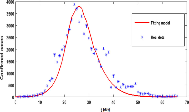
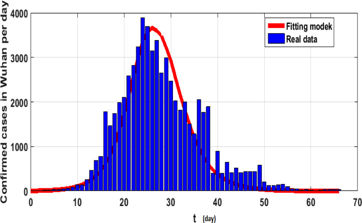
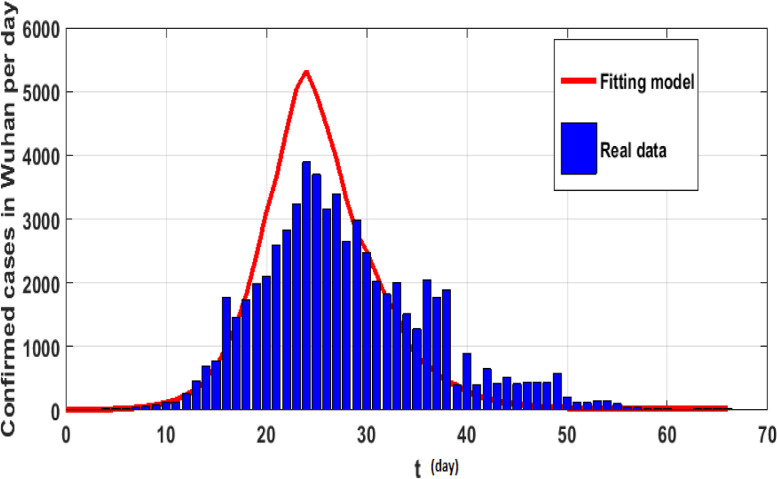
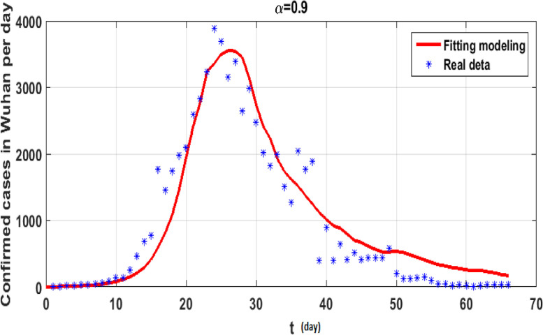
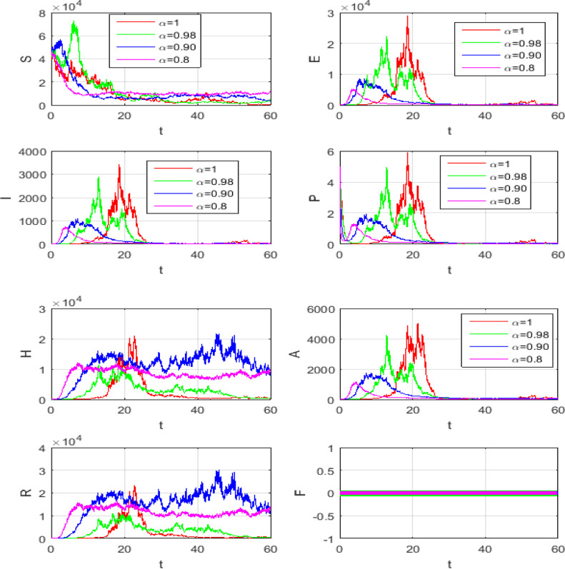
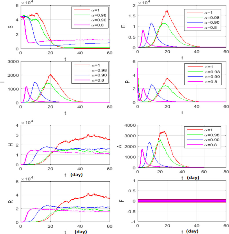
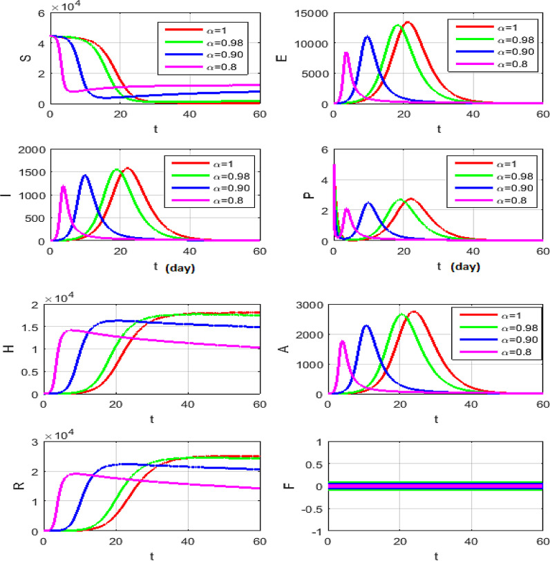
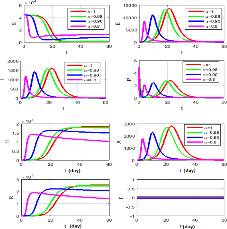
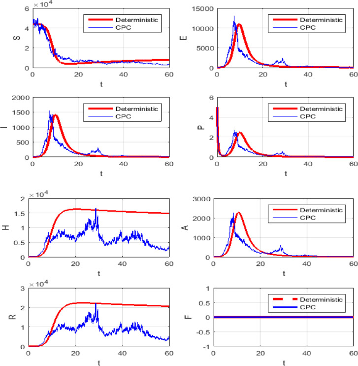
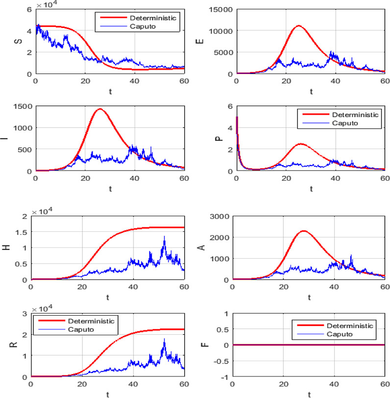
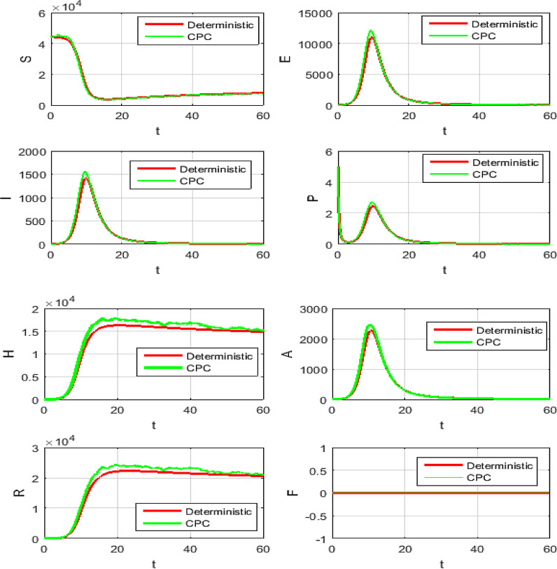
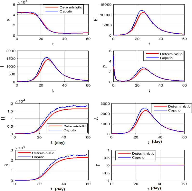
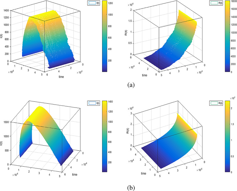
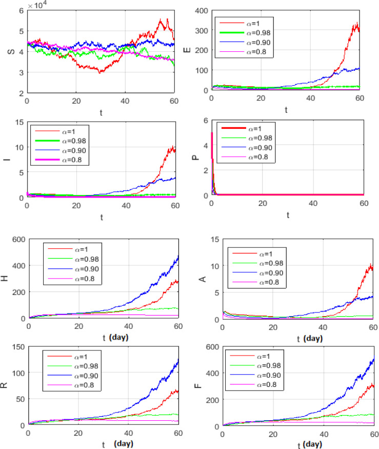
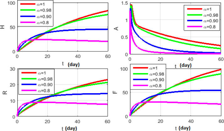
The simulations will be run 100,000 iterations in order to examine the inclusion of stochastic effects into deterministic model. Fig. 1 shows the comparison between real data from WHO verses present considered model at $\sigma =0,$ $\alpha =1$. From this figure, it can be noticed that our model shows a strong agreement with real data collected by WHO during the two months outbreak (66 days to be precise, from January 4 to March 9, 2020)[18]. Also, Fig. (2) -(3 ) show the comparison between real data from WHO verses present considered model at different values of $\sigma .$ Moreover, Fig. 4 shows the comparison between real data from WHO verses present considered model at $\sigma =0.1,$ $\alpha =0.9$. From Fig. 5, Fig. 6, Fig. 7, Fig. 8, Fig. 9, Fig. 10, Fig. 11, Fig. 12, Fig. 13 , we consider ${\delta }_i={\delta }_h={\delta }_p=0,$ with different values of $\sigma$. Fig. 5, Fig. 6, Fig. 7, Fig. 8, show how the solutions are changed with different values of the order $\alpha$.

Fig. 1.

Real data verses model (7) fitting at $\alpha =1,$ and $\sigma =0.0$.

Fig. 2.

Real data verses model (7) fitting at $\alpha =1,$ and $\sigma =0.05$.

Fig. 3.

Real data verses model (7) fitting at $\alpha =1,$ and $\sigma =0.1$.

Fig. 4.

Real data verses model (7) fitting and $\sigma =0.1$.

Fig. 5.

Mean solution for the model (7) at different $\alpha ,$$T_f=60,$${\delta }_i={\delta }_h={\delta }_p=0$ and $\sigma =0.5$.

Fig. 6.

Mean solution for the model (7) at different $\alpha ,$$T_f=60,$${\delta }_i={\delta }_h={\delta }_p=0$ and $\sigma =0.1$.

Fig. 7.

Mean solution for the model (7) at different $\alpha ,$$T_f=60,$${\delta }_i={\delta }_h={\delta }_p=0$ and $\sigma =0.005$.

Fig. 8.

Mean solution for the model (7) at different $\alpha ,$$T_f=60,$${\delta }_i={\delta }_h={\delta }_p=0$ and $\sigma =0$.

Fig. 9.

Mean solution for the model (7) at $\alpha =0.9,$$T_f=60,$${\delta }_i={\delta }_h={\delta }_p=0$ and $\sigma =0.6$.

Fig. 10.

Mean solution for the model (7) at $\alpha =0.9,$$T_f=60,$${\delta }_i={\delta }_h={\delta }_p=0$ and $\sigma =0.6$.

Fig. 11.

Mean solution for the model (7) at $\alpha =0.9,$$T_f=60,$${\delta }_i={\delta }_h={\delta }_p=0$ and $\sigma =0.06$.

Fig. 12.

Mean solution for the model (7) at $\alpha =0.9,$$T_f=60,$${\delta }_i={\delta }_h={\delta }_p=0$ and $\sigma =0.06$.

Fig. 13.

Mean solution for the model (7) at $\alpha =0.9,$$T_f=60,$${\delta }_i={\delta }_h={\delta }_p=0$ at $\sigma =0.09$ in (a) and $\sigma =0.009$ in (b).

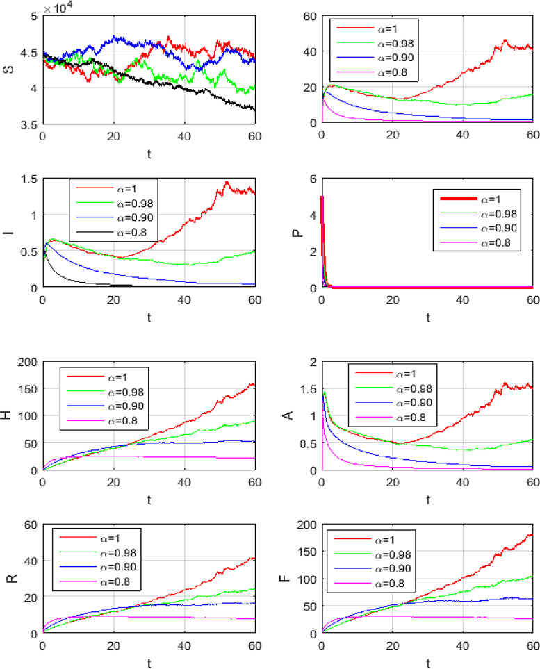
Figs. (9) to (12) show the level of noises at different values of $\sigma$ and $\alpha =0.9$ by using (10) and (11). Comparing the results obtained from Fig. 11 with Fig. 12 at the same data, we can claim that the results which obtained by Fig. 11 is the best, because these result is more convergent to the deterministic case than the results which obtained with Caputo operator. Fig. 13 shows the numerical simulations in 3 dimensions of the mean solutions for $I$ and $R$ at $\sigma =0.09,$ $\alpha =0.9$ in Fig. 13 (a) and $\sigma =0.009,$ $\alpha =0.9$ in Fig. 13 (b). In Fig. 14, Fig. 15, Fig. 16 , we considered ${\delta }_i,$ ${\delta }_h$ and ${\delta }_p,$ not equal zero as in Table 2. These figures, show how the level of noises change at different values of $\sigma$ and $\alpha$. All computations are done using MATLAB.

Fig. 14.

Mean solution for the model (7) at different $\alpha ,$$T_f=60$ and $\sigma =0.1$.

Fig. 15.

Mean solution for the model (7) at different $\alpha ,$$T_f=60$ and $\sigma =0.05$.

Fig. 16.

Mean solution for the model (7) at different $\alpha ,$$T_f=60$ and $\sigma =0$.

6. Conclusions

In this work, the HFSCM is presented, where the new CPC operator which given in [9] is successfully used to constructed the proposed Coronavirus model. The proposed stochastic COVID-19 model describes well the real data of daily confirmed cases in Wuhan. This model shows a strong agreement with real data collected by WHO [18]. The model provides new insights into epidemic-logical situations when the environmental noise (perturbations) and fractional calculus are considered in the COVID-19 model. The combination of white noise and fractional order in the epidemic model, has a considerable impact on the persistence and extinction of the infection and enriches the dynamics of the model.

Milstein’s method is constructed with the new operator to simulate the model problem. The mean-square stability is given. Numerical simulations in this article are implemented for different $\sigma$ and $\alpha$. We concluded that the level of noise reduced when the value of $\sigma$ convergent to zero. From our results which obtain in this article we concluded that the proposed hybrid operator derivative is more general and suitable to study the Coronavirus model than the Caputo’s derivative. Some simulations are presented to support our theoretical findings. Finally, we suggest that the CPC derivative could be useful for the scientists and researchers.

Credit authorship contribution statement

This is a joint paper. All the manuscript works are done in an equal percentage of participation. The author(s) read and approved the final manuscript.

Declaration of Competing Interest

The authors have declared no conflict of interest.

References

- 1.Baleanu D., Mohammadi H., Rezapour S. A fractional differential equation model for the COVID-19 transmission by using the caputo fabrizio derivative. Advances in Difference Equations. 2020;299 doi: 10.1186/s13662-020-02762-2. [DOI] [PMC free article] [PubMed] [Google Scholar]; 10.1186/s13662-020-02762-2
- 2.Podlubny I. Fractional differential equations. Academic Press, New York, 1999 [Google Scholar]
- 3.Carvalho A.R.M., Pinto C.M.A. Non-integer order analysis of the impact of diabetes and resistant strains in a model for TB infection. Commun Nonlinear Sci Numer Simulat, 2018;61:104–126. [Google Scholar]
- 4.Sweilam N.H., AL-Mekhlafi S.M., Hassan A.N. Numerical treatment for solving the fractional two-group influenza model. Progr Fract Differ Appl, 2018;4 [Google Scholar]; 15–1
- 5.Kumar S., Ghosh S., Lotayif M.S.M., Samet B. A model for describing the velocity of a particle in brownian motion by robotnov function based fractional operator. Alexandria Eng J. 2020 [Google Scholar]; https://doi.org/10.1016/j.aej.2020.04.019
- 6.Rihan F.A., Baleanu D., Lakshmanan S., Rakkiyappan R. On fractional SIRC model with salmonella bacterial infection. Abstract and Applied Analysis. 2014:1–9. [Google Scholar]
- 7.Machado J.A.T. Fractional-order derivative approximations in discrete-time control systems. Syst Anal Model Simul. 1999;34:419–434. [Google Scholar]
- 8.Dehghan M., Hamedi E., Khosravian-Arab H. A numerical scheme for the solution of a class of fractional variational and optimal control problems using the modified jacobi polynomials. Journal of Vibration and Control. 2016;22:1547–1559. [Google Scholar]
- 9.Baleanu D., Fernandez A., Akgül A. On a fractional operator combining proportional and classical differintegrals. mathematics. 2020;8(3) doi: 10.3390/math8030360. [DOI] [Google Scholar]
- 10.Brauer F., Driessche P., Wu J. Springer; 2008. Mathematical epidemiology. [Google Scholar]
- 11.World health organization. 2020a. Available: https://www.who.int/health-topics/coronavirus.Coronavirus. World Health Organization, cited January 19.
- 12.Ndärou F., Area I., Nieto J.J., Torres D.F.M. Mathematical modeling of COVID-19 transmission dynamics with a case study of wuhan. Chaos, Solitons and Fractals. 2020 doi: 10.1016/j.chaos.2020.109846. [DOI] [PMC free article] [PubMed] [Google Scholar]
- 13.H. Sweilam N., AL-Mekhlafi S.M., Baleanu D. A hybrid fractional optimal control for a novel coronavirus (2019-ncov) mathematical model. Journal of Advanced Research, 2020 doi: 10.1016/j.jare.2020.08.006. [DOI] [PMC free article] [PubMed] [Google Scholar]
- 14.Khan M.A., Atangana A. Modeling the dynamics of novel coronavirus (2019-ncov) with fractional derivative. Alexandria Engineering Journal, 2020 doi: 10.1016/j.aej.2020.02.033. [DOI] [Google Scholar]
- 15.Chen T.-M., Rui J., Wang Q.-P., Zhao Z.-Y., Cui J.-. A., Yin L.. A mathematical model for simulating the phase-based transmissibility of a novel coronavirus. 2020. 9–24, 10.1186/s40249-020-00640-3 [DOI] [PMC free article] [PubMed]
- 16.Ivorra B., Ferrández M.R., Vela-Pérez M., Ramos A.M. Mathematical modeling of the spread of the corona virus disease 2019 (COVID-19) taking into account the undetected infections. The case of China. 2020 doi: 10.13140/RG.2.2.21543.29604. [DOI] [PMC free article] [PubMed] [Google Scholar]
- 17.Scherer R., Kalla S., Tang Y., Huang J. The grünwald-letnikov method for fractional differential equations. Comput Math Appl, 2011;62:902–917. [Google Scholar]
- 18.COVID-19 coronavirus pandemic. 2020b. https://www.worldometers.info/coronavirus/repro, Accessed March 26.
- 19.Sweilam N.H., Hasan M.M.A., Baleanu D. New studies for general fractional financial models of awareness and trial advertising decisions. Chaos, Solitons and Fractals. 2017;104:772–784. [Google Scholar]
- 20.Aguila-Camacho N., Duarte-Mermoud M.A., Gallegos J.A. Lyapunov functions for fractional order systems. Commun Nonlinear Sci Numer Simul. 2014;19 [Google Scholar]; 2951?2957
- 21.Talay D., Tubaro L. Expansion of the global error for numerical schemes solving stochastic differential equations. Stoc Anal Appl, 1990;8:483–509. [Google Scholar]
- 22.He S., Tang S., Rong L. discrete stochastic model of the COVID-19 outbreak: Forecast and control. MBE. 2020;17(4):2792–2804. doi: 10.3934/mbe.2020153. [DOI] [PubMed] [Google Scholar]
- 23.Chatterjee K., Chatterjee K., Kumar A., Shankar S. Healthcare impact of COVID-19 epidemic in india: A stochastic mathematical model. MJFAI. 2020;76:147-155. doi: 10.1016/j.mjafi.2020.03.022. [DOI] [PMC free article] [PubMed] [Google Scholar]
- 24.Karako K., Song P., Chen Y., Tang W. Analysis of COVID-19 infection spread in japan based on stochastic transition model. BioScience Trends Advance Publication. 2020 doi: 10.5582/bst.2020.01482. [DOI] [PubMed] [Google Scholar]
- 25.Watmough P., Driessche P. Reproduction numbers and sub-threshold endemic equilibria for compartmental models of disease transmission. Math Biosci. 2002;180:29–48. doi: 10.1016/s0025-5564(02)00108-6. [DOI] [PubMed] [Google Scholar]
- 26.Hasminskii R.Z. Springer; Berlin: 1980. Stochastic stability of differential equations. [Google Scholar]
- 27.Atangana A., Araz S.I. Nonlinear equations with global differential and integral operators: Existence, uniqueness with application to epidemiology. Results in Physics. 2021;20 doi: 10.1016/j.rinp.2020.103593. [DOI] [PMC free article] [PubMed] [Google Scholar]
- 28.Atangana A., Araz S.I. Mathematical model of COVID-19 spread in turkey and south africa: Theory, methods and applications. Advances in Difference Equations. 2020;659 doi: 10.1101/2020.05.08.20095588. [DOI] [PMC free article] [PubMed] [Google Scholar]
- 29.Atangana A. Modelling the spread of COVID-19 with new fractal-fractional operators: Can the lock down save mankind before vaccination. Chaos, Solitons & Fractals. 2020;136:109860. doi: 10.1016/j.chaos.2020.109860. [DOI] [PMC free article] [PubMed] [Google Scholar]