Polygenic Selection within a Single Generation Leads to Subtle Divergence among Ecological Niches

Abstract

Selection on standing genetic variation may be effective enough to allow for adaptation to distinct niche environments within a single generation. Minor allele frequency changes at multiple, redundant loci of small effect can produce remarkable phenotypic shifts. Yet, demonstrating rapid adaptation via polygenic selection in the wild remains challenging. Here we harness natural replicate populations that experience similar selection pressures and harbor high within-, yet negligible among-population genetic variation. Such populations can be found among the teleost Fundulus heteroclitus that inhabits marine estuaries characterized by high environmental heterogeneity. We identify 10,861 single nucleotide polymorphisms in F. heteroclitus that belong to a single, panmictic population yet reside in environmentally distinct niches (one coastal basin and three replicate tidal ponds). By sampling at two time points within a single generation, we quantify both allele frequency change within as well as spatial divergence among niche subpopulations. We observe few individually significant allele frequency changes yet find that the “number” of moderate changes exceeds the neutral expectation by 10–100%. We find allele frequency changes to be significantly concordant in both direction and magnitude among all niche subpopulations, suggestive of parallel selection. In addition, within-generation allele frequency changes generate subtle but significant divergence among niches, indicative of local adaptation. Although we cannot distinguish between selection and genotype-dependent migration as drivers of within-generation allele frequency changes, the trait/s determining fitness and/or migration likelihood appear to be polygenic. In heterogeneous environments, polygenic selection and polygenic, genotype-dependent migration offer conceivable mechanisms for within-generation, local adaptation to distinct niches.

Significance

Natural selection allows organisms to adapt to novel environmental conditions over just a few generations, yet the underlying mechanisms allowing for rapid and repeated adaptation remain elusive. One possible explanation is that selection acts, not by removing a deleterious allele at a single gene of large effect but by subtle changes at many genes, each with a minor effect on an adaptively important trait. Here we show that populations inhabiting distinct environmental niches exhibit subtle, yet significant changes at many positions in the genome within a single generation, and that these changes lead to genetic differentiation among niches. Subtle changes at multiple genes of small effect may allow organisms to adapt to specific niches over just a single generation.

Introduction

Can natural selection lead to adaptation on ecological timescales? Can populations respond to environmental challenges within generations or among well-connected demes, allowing them to adapt to their local, heterogeneous, and unstable environments (Hairston et al. 2005; Hendry et al. 2007; Richardson et al. 2014; Messer et al. 2016)? For decades, the consensus among evolutionary biologists was “No.” Evolutionary adaptation on ecological scales is unlikely due to fundamental limits on the extent of selectively important allelic variation and the rate of adaptive change (Haldane 1957; Kimura 1968; Lewontin 1974; Orr 2005). Yet, an ever increasing number of studies demonstrate adaptation on both short temporal (Bergland et al. 2014; Gompert et al. 2014; Stuart et al. 2014; Paccard et al. 2018; Barrett et al. 2019; Dayan et al. 2019) and small spatial scales (Williams and Oleksiak 2011; Fraser et al. 2015; Reid et al. 2016; Wagner et al. 2017). These observations conflict with the predictions of classic, mutation-limited adaptation. Fortunately, adaptation via selection on standing genetic variation offers a tangible solution to this problem (Barrett and Schluter 2008). Selection on alleles already segregating in a population can readily effect phenotypic change, however, their importance and prevalence is hotly debated (Kreitman 1996; Harris et al. 2018; Kern and Hahn 2018; Jensen et al. 2019). For instance, selective sweeps rapidly erode genetic variation, especially when the selected trait has a nonredundant, mono- or oligogenic architecture (Hermisson and Pennings 2005; Przeworski et al. 2005). In highly heterogeneous environments with alternating selection pressures, successive sweeps will therefore erode the genetic variation upon which they act, making adaptation from standing genetic variation unsustainable in the long term (Rockman 2012).

Under a polygenic framework, in which redundancy allows for multiple genetic solutions to effect a phenotypic change, adaptation only requires slight allele frequency changes at a subset of potentially adaptive loci that are already segregating in the population (Pritchard and Di Rienzo 2010; Pritchard et al. 2010; Yeaman 2015; Sella and Barton 2019). The advantages of redundant, polygenic adaptation are manifold as follows: 1) selection on standing genetic variation is highly effective and can occur within a single generation, 2) polymorphism and therefore future adaptive potential is largely maintained, and 3) adaptation is less sensitive to migration because gene flow promotes genetic variation upon which polygenic selection can act (Przeworski et al. 2005; Pritchard and Di Rienzo 2010; Pritchard et al. 2010; Yeaman 2015; Barton et al. 2017; Wittmann et al. 2017; Barton and Etheridge 2018; Sella and Barton 2019).

However, demonstrating redundant, polygenic adaptation in a natural setting is inherently challenging (Latta 1998; Le Corre and Kremer 2003, 2012; Yeaman 2015). First, phenotypic variance is split among multiple loci, thereby reducing per-locus effect size. This implies allele frequency changes in response to selection will also be minor and difficult to identify and distinguish from neutral drift or demographic effects (Harris et al. 2018; Barton et al. 2019; Berg et al. 2019; Sohail et al. 2019; Johri et al. 2020; Whiting and Fraser 2020). Second, genetic redundancy implies that the number of allelic variants required to reach a local phenotypic optimum (n_opt) is much lower than the total number of variants affecting a trait (n_tot), that is, n_opt ≪ n_tot (Nowak et al. 1997; Yeaman 2015). Hence, unique subsets of redundant alleles may equally lead to local adaptation in replicate populations (Latta 1998; Le Corre and Kremer 2003, 2012; Yeaman 2015; Reid et al. 2016). Third, as per-locus, additive effect sizes decrease, gene-by-gene interactions must be increasingly responsible for any phenotypic effect (Latta 1998; Le Corre and Kremer 2003, 2012). Consequently, it is unlikely that natural selection will alter the same loci among replicate populations or in replicate experiments exposed to the same selection pressures (Yeaman 2015). Distinguishing adaptive allele frequency changes from stochastic changes due to, for example, drift is therefore extremely challenging, especially given the countless theoretical models in which certain parameterizations of demography, mutation rates, and background selection are shown to create genomic patterns typically associated with selection on standing genetic variation (Harris et al. 2018; Sella and Barton 2019; Johri et al. 2020).

We are beginning to explore polygenic selection and redundancy in laboratory settings by employing massively parallel, experimental selection (Barghi et al. 2019); however, studies pursuing redundant, polygenic adaptation in nature are rare and mostly human focused (Pritchard et al. 2010; Berg and Coop 2014). Here, we harness the Fundulus heteroclitus model system to demonstrate redundant, polygenic adaptation occurring at extremely small temporal and spatial scales in the wild. Fundulus heteroclitus, a small, marine teleost, native to the eastern coast of the United States, primarily inhabits tidal estuaries and demonstrates extremely high site fidelity to a single watershed (Lotrich 1975; Skinner et al. 2005, 2012; Able et al. 2012). Within these estuaries exist several, unique niches (or microhabitats), each characterized by distinct biotic and abiotic factors such as temperature, dissolved oxygen, or predator abundance (Able 1984; Able and Felley 1986; Smith and Able 2003; Hunter et al. 2007, 2009; Kimball and Able 2012). Fundulus heteroclitus inhabit the entire estuary and demonstrate some degree of site fidelity to specific niches, thus forming multiple subpopulations within the larger population. Nevertheless, fish from across the estuary reproduce at a common location on a yearly basis (Taylor et al. 1979), essentially homogenizing allele frequencies and maintaining panmixia.

Contrary to the prediction that panmictic breeding inhibits local adaptation, previous work identified significant genetic divergence among F. heteroclitus inhabiting distinct niches <100 m apart in three replicate estuaries/populations (Wagner et al. 2017). The authors identified single nucleotide polymorphisms (SNPs) displaying significant spatial differentiation among well-connected niches in each of three isolated estuaries and supported by three different selection tests. Although none of the outlier loci were shared among all three replicate populations, many SNPs occur either 1) within the same gene at a different position, 2) in a duplicate gene or paralog, or 3) among genes that share narrow, well-defined Gene Ontology (GO) terms (Wagner et al. 2017). That is, although no outlier SNPs were shared among the three replicate populations, there were signals of selection in the same gene or genes of similar function, a hallmark of redundancy. The authors concluded that redundant, polygenic selection was surprisingly effective in altering allele frequencies among multiple, distinct SNPs that likely share similar biological functions in response to environmental and ecological differences over very small geographic distances. Yet, it remains difficult to believe that significant genetic divergence among well-connected niches results from repeated, within-generation selection rather than assortative mating or active, phenotype-dependent niche sorting.

Our study builds on prior work and tests for within-generation local adaptation in a single, panmictic F. heteroclitus population by harnessing both spatial and temporal data. We specifically examine subpopulations residing in distinct niches and quantify temporal allele frequency changes within a single generation from spring to fall, when natural mortality is highest (Kneib 1993). We find both the number and magnitude of within-generation allele frequency changes to be beyond what is expected by neutral drift. Analyses are strengthened further by detecting significant concordance in both the magnitude and direction of allele frequency changes among subpopulations. Finally, we show that within-generation allele frequency changes generate subtle, yet significant, divergence among subpopulations, suggestive of fine scale, local adaptation to distinct niche environments within a single generation. On a “per-locus” basis we find only few individually significant loci, yet the “total number” of loci demonstrating substantial allele frequency change in time and divergence among niches is significantly elevated, suggestive of a polygenic architecture. Hence, although the signal is moderate, as is expected given the limitations of testing for polygenic selection, the data presented here support the hypothesis of local adaptation within a single generation.

Materials and Methods

Tagging and Sample Collection

Initial tagging and tissue collection took place in late spring 2016 (22 May–5 June) at the Rutgers University Marine Field Station (RUMFS), NJ. Over a 10-day period, 2,200 F. heteroclitus were caught using minnow wire traps at four sampling sites (550 fish per site) throughout a single saltmarsh estuary (fig. 1). The collection sites included a coastal basin and three permanent, intertidal ponds, all part of the same watershed and interconnected during spring tides occurring ∼5–15 times per month (Hunter et al. 2007, 2009).

Fig. 1.

Location of the four sampling sites within the watershed around the Rutgers University Marine Field Station (RUMFS). Inset shows the location of the RUMFS on the coast of New Jersey, USA.

Five hundred fish from each sampling site were weighed, measured (total length), sexed, and uniquely tagged using sequential coded wire tags (Northwest Marine Technology Inc., Shaw Island, WA). Caudal fin clips were taken from the remaining 50 fish and stored in guanidinium hydrochloride (GuHCl) buffer solution. After tagging/clipping, fish were released at their respective capture location. Tagged fish were recaptured in early fall 2016 (30 August–10 September) by trapping at the same four collection sites. Trapping efforts were continued until 50 tagged fish had been recaptured at each location (only 45 were recaptured in the basin). Recaptured, tagged fish were weighed, measured (total length), and sexed. Caudal fin clips were taken from all 195 recaptured fish and stored in GuHCl buffer solution. Coded wire tags were dissected from each individual and cross-referenced with spring tagging data. Only residents, that is, fish that were tagged and recaptured at the same location, were included in further analysis. This sampling scheme allowed for spatial comparisons among sampling sites as well as assessment of temporal change from spring to fall. Although summer residency does not implicate genetic, ecological, or reproductive substructure, for the purpose of this analysis, resident individuals from a single collection site are henceforth collectively referred to as a subpopulation. Differences in length and growth rate among subpopulations were assessed using Kruskal–Wallis tests followed by post hoc, Mann–Whitney U tests in R v3.6.1. Weight data were excluded due to the high abundance of gravid females during spring collection that may have confounded results.

DNA Isolation and Library Preparation

Genomic DNA was isolated from 30 individuals from each resident subpopulation and time point (spring and fall) using a custom SPRI magnetic bead protocol, yielding a total of 240 isolates. Genotyping-by-sequencing (GBS) libraries were prepared using a modified protocol after Elshire et al. (2011). Briefly, high molecular weight genomic DNA was aliquoted and digested using AseI restriction enzyme. Digests from each sample were uniquely barcoded, pooled, and size selected to yield insert sizes between 350 and 550 bp. Pooled libraries were amplified using custom primers that extend into the insert by one base (cytosine). This approach systematically reduces the number of sequenced GBS tags, ensuring sufficient sequencing depth.

Sequencing and SNP Calling

Pooled libraries were sequenced on one lane of the Illumina HiSeq 4000 in 2 × 150 bp paired-end mode yielding ∼467 million paired-end reads (>140 Gb). Reads were aligned to the Fundulus_heteroclitus-3.0.2 reference genome (NCBI RefSeq accession number: GCF_000826765.1), and single nucleotide polymorphisms (SNPs) were called using the GBeaSy analysis pipeline (Wickland et al. 2017) with the following filter settings: minimum read length of 30 bp after barcode and adapter trimming, minimum phred-scaled variant quality of 30, and minimum read depth of 5 at the sample level. This yielded a total of 2,393,661 SNPs that were further filtered using VCFtools 0.1.13. Specifically, only biallelic SNPs without extreme heterozygote excess (q value > 0.01) were included. Although within-generation selection may cause departures from Hardy–Weinberg equilibrium (HWE), removing loci with extreme heterozygote excess excludes artifacts resulting from the alignment of paralogous sequences. While this conservative filter may have excluded potentially interesting loci, it effectively removed only 6.4% of SNPs (supplementary table S1, Supplementary Material online). SNPs were further filtered to a maximum of 10% missing data and a minimum minor allele frequency of 5%. Filtering was also applied at the sample level to only include individuals with more than 60% completeness, that is, <40% missing genotypes per sample. To minimize the confounding effect of linkage disequilibrium (LD), the variant set was thinned to a minimum of 300 bp between SNPs (see supplementary fig. S2, Supplementary Material online). The final, filtered set contained 193 individuals genotyped at 10,861 SNPs. Sample sizes by location and season remained relatively balanced following filtering (spring:fall = 86:107; Basin:Pond 1:Pond 2:Pond 3 = 51:46: 49:47). Here, “allele frequency” refers to the frequency of the F. heteroclitus reference genome allele. Because only biallelic SNPs were used in the analysis, the alternate allele frequency is implied.

Within-generation Allele Frequency Change and Niche Divergence

Global and pairwise F_ST statistics were calculated using VCFtools v0.1.13. Principal component analysis (PCA) was performed in R v3.6.1 using SNPRelate v1.18.1. p values quantifying the significance of spatial (i.e., among sites) and temporal (i.e., between seasons) allele frequency differences/changes were attained via three distinct tests. These were as follows: 1) a permutation analysis, 2) a simulation approach, modeling neutral drift and sampling variance, and 3) a Barnard’s exact test.

Permutations were performed using a custom, parallelized bash script. Briefly, p values were generated by comparing empirical F_ST values, either between sites in fall (spatial) or between seasons (temporal), to permuted values conditioned on heterozygosity as in FDIST2 (Beaumont and Nichols 1996), that is, only SNPs of similar heterozygosity (H_E ± 0.0025) were compared. Samples from all locations and both time points were permuted in order to increase permutation space and decrease the likelihood of generating sets that match empirical data.

Simulations of neutral drift and sampling variance were generated to test for significant allele frequency changes from spring to fall (R v3.6.1). Specifically, for every subpopulation, spring and fall empirical data were considered two samples of a temporally invariant population. For every SNP, the weighted mean allele frequency of spring and fall samples was used to simulate a subpopulation in HWE. Simulated subpopulations were then randomly sampled n_i times without replacement, where n is the empirical sample size at each SNP at time point i. Random sampling of the simulated subpopulations is representative both of random death in the wild as well as experimental sampling effects in the field and during sequencing. This yielded a simulated “spring” and “fall” sample from which apparent temporal allele frequency change was calculated. Ten thousand Monte Carlo iterations were performed per SNP, generating SNP-specific distributions of apparent allele frequency change under the null hypothesis of neutral drift. By conducting SNP-specific simulations, the empirical allele frequency, which conditions the magnitude of allele frequency change, is accounted for. Empirical allele frequency changes were then compared with the simulated distributions and p values generated according to rank. Independent simulations were produced for every subpopulation in order to account for potential genetic structure. Simulated subpopulation sizes were 1,300 and 400 for the basin and ponds, respectively. These estimates are based on the observed F. heteroclitus abundance in the wild, determined by exhaustively trapping at each collection site until no further fish were captured for two consecutive trapping periods of 4 h each.

Simulations testing significant spatial allele frequency differences were conducted in a similar fashion. Here, SNP-specific populations were generated under the null hypothesis of spatial homogeneity. Subpopulations were considered samples of a single, panmictic, population and their weighted mean allele frequency used to simulate a metapopulation in HWE. Distributions of apparent allele frequency differences in the absence of spatial structure were generated by repeatedly sampling (10,000 Monte Carlo iterations) the simulated metapopulation with sample sizes n_j, where j indicates the specific subpopulation. Empirical allele frequency differences among subpopulations were compared with the distribution of apparent allele frequency differences under panmixia and p values generated as above. Spatial simulations were only conducted on fall data in order to remain agnostic to potential temporal change.

Barnard’s exact test was performed on contingency tables of allele counts comparing either temporal changes (within each subpopulation) or pairwise spatial differences (fall only). Barnard’s test is statistically similar to Fisher’s exact test and, while computationally more demanding, better suited to genetic data because it does not condition on margin totals. Tests were performed using the Exact package in R v3.6.1.

To facilitate further analysis, p values from the permutation approach, simulation analysis, and Barnard’s tests were combined by taking their geometric mean. The geometric mean is a conservative aggregation method, appropriate for combining highly correlated p values, where Spearman’s ρ > 0.9 (Vovk and Wang 2020) (supplementary fig. S3, Supplementary Material online). This resulted in a single p value per SNP and subpopulation, quantifying the significance of temporal allele frequency change, as well as a single p value per SNP and pairwise comparison, quantifying the significance of spatial differentiation in fall. Multiple test correction was performed using the p.adjust function in R v3.6.1 by applying both the false discovery rate (FDR = 10%) and nonsequential Bonferroni methods.

Temporal Concordance

A Cochran–Mantel–Haenszel (CMH) test was applied to temporal data in order to determine whether allele frequency changes were significantly concordant among niches, specifically ponds, and hence likely due to selection. The CMH test assesses the degree of concordance with respect to both magnitude and direction of allele frequency change. Concordance was tested as follows: 1) among all four subpopulations, 2) among the three ponds only, and 3) among every other three-way combination, for example, Basin:Pond 1:Pond 2. To assess the degree of spurious concordance, CMH tests were also performed on 1,000 simulations of temporally invariant subpopulations (see above for details). Tests were performed on contingency tables of allele counts using the mantel.haenszel function in R v3.6.1.

Results

Phenotypic Divergence yet Negligible Population Structure

Of the 2,000 fish tagged in spring 2016, 195 (9.8%) were successfully recaptured in the fall of the same year. Recaptured F. heteroclitus demonstrated high site fidelity with 186 (95.4%) individuals recaptured at their respective tagging site. Nine migrant fish were excluded from further analysis.

Fundulus heteroclitus subpopulations displayed significant body length differences in spring (Kruskal–Wallis, P ≪ 0.05) (fig. 2A), with Basin individuals exhibiting the highest mean total length. The bimodal length distribution of all subpopulations suggests the presence of two cohorts of different ages (supplementary fig. S4, Supplementary Material online). In the Basin subpopulation, the proportion of larger and likely older fish is substantially higher than in the ponds. The reason for this asymmetric age structure is unclear but could potentially be due to increased mortality of larger (i.e., older) fish in the ponds. Growth rates, calculated for recaptured individuals only, were also significantly different among locations (Kruskal–Wallis, P ≪ 0.05) (fig. 2B). Notably, although Basin residents show marginally higher growth rates when grouping individuals from all ponds (Mann–Whitney U, P = 0.058), this result is driven by significant variation among distinct ponds (Mann–Whitney U, P < 0.05). In fact, Pond 1 residents exhibit the same growth rate as Basin residents (Mann–Whitney U, P = 0.52), suggesting each pond may present unique environmental conditions leading to distinct growth profiles (Stuart et al. 2017).

Fig. 2.

Significant phenotypic differences among subpopulations. Box plots showing total length of tagged fish in spring (A) and growth rate of recaptured individuals as a percentage of spring total length. (B) Global Kruskal–Wallis tests are highly significant for both spring length and growth. Post hoc, pairwise comparisons are displayed as lowercase letters; subpopulations with the same letter are not significantly different (Wilcoxon, P > 0.05).

Despite high site fidelity, F. heteroclitus show negligible population structure based on all 10,861 SNPs, with a global, mean weighted F_ST among all subpopulations and time points of 8.5 × 10⁻⁴. A PCA biplot using all 10,861 SNPs (supplementary fig. S5, Supplementary Material online) shows negligible structure in both space (i.e., among sampling sites) and time (i.e., between seasons). The absence of spatial structure is expected in a highly connected population with yearly panmictic breeding. Likewise, the lack of a temporal signal between spring and fall collections suggests no major allele frequency shifts, expected for populations near equilibrium. Consequently, any signal is likely to be moderate and limited to a minor subset of alleles.

Significant Within-generation Allele Frequency Changes

Resident fish are assumed to have been exposed to their niche-specific environments and associated selection pressures during summer. Selective death or genotype-dependent emigration will therefore be reflected in significant allele frequency changes relative to the spring sample.

The significance of temporal allele frequency change was quantified by the geometric mean p value, summarizing three separate significance tests (Barnard’s test, permutation, and simulation analyses) (fig. 3). This approach yielded 611 significant allele frequency changes in the Basin, 664 in Pond 1, 571 in Pond 2, and 625 in Pond 3 (geometric mean p < 0.05), unlikely due to sampling error, random death, or random emigration. However, these totals narrowly exceed the expected number of false positives under a uniform p value distribution (5% of 10,861 = 543). In fact, only two SNPs within Pond 1 remain significant after multiple test correction (red points, fig. 3). SNPs that were significant at an FDR of 10% are also significant at the Bonferroni level and are hence displayed as the latter. The absence of major, temporal allele frequency changes paired with a moderately elevated “number” of significant SNPs is suggestive of widespread allele frequency changes of small effect, a pattern associated with polygenic selection (Latta 1998; Le Corre and Kremer 2003, 2012).

Fig. 3.

Significant within-generation allele frequency changes in each subpopulation. Temporal change in the reference allele frequency and associated p value for all 10,861 SNPs. p values shown are the geometric mean of p values generated from three separate significance tests (Barnard’s test, permutation, and simulation). SNPs with a significant allele frequency change are shown in color (blue, p < 0.05; red, Bonferroni corrected). Gray contour lines show the high density of loci with insignificant allele frequency changes.

To further investigate this idea, the observed number of significant allele frequency changes was compared with the expected number of significant allele frequency changes under neutral drift (see Gompert et al. 2014; Barrett et al. 2019 for a similar approach). Figure 4 shows the observed to expected (O:E) ratio of significant allele frequency changes evaluated across a spectrum of alpha levels to determine the excess of significant allele frequency changes at both moderate and strict significance thresholds. Whereas Pond 2 predominantly falls within the 95% confidence interval of neutral drift, the observed number of significant allele frequency changes in Basin, Pond 1, and Pond 3 exceeds the neutral expectation at intermediate alpha levels between 10⁻¹ and 10^−2.5. In these subpopulations, we observe 1.1 to 2-fold more SNPs showing significant, temporal allele frequency changes than expected due to random drift and sampling error. However, at lower alpha levels around 10⁻³, only Pond 1 shows a significant O:E ratio. This pattern is indicative of an elevated number of moderate allele frequency changes in the absence of any major shifts as would be expected under polygenic selection (Latta 1998; Le Corre and Kremer 2003, 2012).

Fig. 4.

Number of significant, within-generation allele frequency changes exceeds the neutral expectation. Observed to expected ratio of the number of significant allele frequency changes, evaluated across significance thresholds (alpha levels). The black, solid line marks the expected ratio of 1 under neutral drift. The black, dashed line and gray shading mark the one-tailed 95% confidence interval.

Concordant Allele Frequency Change among Niches

To further test the hypothesis of within-generation, polygenic selection, we assessed the concordance of allele frequency changes in both direction and magnitude, specifically among pond subpopulations that are exposed to similar environmental conditions.

Of the 10,861 SNPs tested, we find three that show significantly concordant allele frequency changes among pond residents at an FDR of 10% with one SNP showing significance at the Bonferroni level. Although this is not overwhelming, pond subpopulations (red line, fig. 5) also display a significantly elevated number of concordant allele frequency changes. The empirical data exceed both the expected number of false positives at any given alpha level as well as 1,000 simulations under neutrality for which concordance is spurious by design (gray lines, fig. 5). The median O:E ratio of neutral simulations falls below the null expectation of 1. This confirms that the CMH test is in fact conservative, strictly controlling Type I error at the expense of Type II error. Nevertheless, the O:E ratio for the number of concordant allele frequency changes among ponds lies well above 1. For instance, at an alpha level of 10⁻² an O:E ratio of 1.6 suggests 60% more SNPs than expected exhibit concordant allele frequency changes among the three ponds over summer.

Fig. 5.

Significant concordance in within-generation allele frequency changes among subpopulations. Observed to expected ratio of the number of significantly concordant allele frequency changes among different combinations of subpopulations (Cochran–Mantel–Haenszel test). Gray lines show 1,000 simulations of concordance among three simulated subpopulations under the null hypothesis of neutral change and no spatial differentiation. The solid, black line shows the median O:E ratio of the neutral simulations, dashed lines encompass 95% of simulations.

Although the unexpectedly large number of concordant SNPs among pond subpopulations is suggestive of niche-specific allele frequency changes resulting from parallel selection, other three-way combinations, which include the basin subpopulation, show similarly elevated O:E ratios (blue shaded lines, fig. 5). In fact, the number of concordant SNPs among all subpopulations (green line, fig. 5) is up to 3-fold higher than expected and exceeds 1,000 neutral simulations, indicative of parallel, ecosystem-wide allele frequency shifts. Of these, two SNPs remain significant after multiple test correction at an FDR of 10% with one showing significance at the Bonferroni level. Significant, concordant allele frequency changes at these loci seem to be unrelated to niche environment and are potentially due to a common selection pressure experienced by all subpopulations.

Fine Spatial Structure among Niche Populations

Although there is negligible spatial structure when utilizing all 10,861 SNPs (supplementary fig. S5, Supplementary Material online), pairwise comparisons among subpopulations in fall yield individual loci with exceptional F_ST values (supplementary fig. S6, Supplementary Material online), often exceeding 0.2 and ranging as high as 0.43. Nevertheless, only two pairwise comparisons yield SNPs that remain significant after multiple test correction; Basin:Pond 2 (two SNPs) and Pond 1:Pond 2 (one SNP) (Bonferroni corrected). Further, Pond:Pond pairwise comparisons yield SNP-specific F_ST values of similar magnitude and significance as Basin:Pond comparisons (supplementary fig. S6, Supplementary Material online), contrary to the prior expectation of genetic divergence among environmentally distinct niches (Wagner et al. 2017).

The results presented here partially corroborate the findings of Wagner et al. (2017) who also found significant spatial outlier SNPs among niches in this and other salt marsh estuaries. However, the authors did not compare within niche type, making it difficult to attribute spatial divergence to a niche effect as opposed to divergence among subpopulations distributed in space. Of the 4,741 SNPs assayed by Wagner et al. (2017), only 115 are successfully genotyped here. The low overlap can be mostly attributed to the filtering required to minimize missing data as well as the thinning approach employed by both studies to avoid inflating outlier numbers due to LD (supplementary table S1 and fig. S2, Supplementary Material online). Nevertheless, of the 63 spatial outlier SNPs identified by Wagner et al. (2017) in 2013, four are present in the current data set of which one shows significant spatial divergence (Basin:Pond 1, p < 0.05).

Perhaps more important than the presence of singular, spatial outlier SNPs is the proportion of SNPs exhibiting significant spatial differentiation compared with the expectation under complete panmixia and neutral drift. Figure 6 shows the ratio of the observed to expected number of significantly differentiated SNPs, evaluated across alpha levels. For every pairwise comparison, the O:E ratio of spatially significant SNPs falls above the neutral expectation for moderate alpha levels between 10⁻¹ and 10⁻². However, at lower alpha levels of 10⁻³ pairwise comparisons yield no more significant, spatial outlier SNPs than expected by the Type I error rate. Hence, although the number of SNPs exhibiting moderate spatial differentiation is elevated beyond what is expected due to neutral processes alone, only few SNPs are individually significantly differentiated. This is indicative of fine, spatial structure among subpopulations, potentially due to weak, polygenic selection. Contrary to prior expectations (Wagner et al. 2017) but consistent with temporal data, Pond:Pond pairwise comparisons yield similar, significantly elevated numbers of spatially diverged SNPs (mean of 635 significant SNPs per pairwise comparison, p < 0.05) as opposed to Basin:Pond comparisons (mean of 638 spatially significant SNPs per pairwise comparison, p < 0.05). Fine, spatial structure within the estuary is therefore likely to be more complex than binary differentiation between two broadly defined niche types (basin vs. pond environments).

Fig. 6.

Number of spatially differentiated SNPs exceeds the neutral expectation. Observed to expected ratio of the number of SNPs showing significant spatial differentiation, evaluated across alpha levels for each pairwise comparison among subpopulations in fall. Basin:Pond pairwise comparisons are displayed on the left, Pond:Pond comparisons on the right. Black solid lines mark the expected ratio of 1 under the null hypothesis of no spatial differentiation. Black, dashed lines and gray shading mark the one-tailed 95% confidence intervals.

Within-generation Allele Frequency Changes Generate Fine Spatial Structure

Both the number of loci exhibiting significant within-generation allele frequency changes, as well as those displaying significant spatial divergence, exceed the neutral expectation. In order to elucidate the spatiotemporal relationship of these non-neutral patterns, we examined the intersection of temporally and spatially significant SNPs. We found a significant enrichment of SNPs that show both a significant allele frequency change over time as well as spatial differentiation (χ² test, p ≪ 0.01). This holds true upon evaluating all temporally significant SNPs, regardless of subpopulation, and all spatially significant SNPs, regardless of pairwise comparison. Significant enrichment also occurs within any given pairwise comparison, that is, when only temporally and spatially significant SNPs pertaining to the subpopulations in a specific pair are taken into account (χ² test, p ≪ 0.01 for all pairwise comparisons). This suggests that within-generation allele frequency changes during summer generate fine spatial structure among subpopulations.

Figure 7 displays the within-generation allele frequency changes of 788 SNPs that exhibit significant spatial divergence in fall (geometric mean p < 0.01). To simplify visualization, data from all six pairwise comparisons were collapsed into a single graphic. The x and y axes display temporal allele frequency change for any arbitrary pair of subpopulations. The coloration indicates the spatial differentiation among these subpopulations in fall (see supplementary fig. S7, Supplementary Material online, for specific pairwise comparisons). Spatially diverged SNPs have a bimodal distribution and are largely found in the upper left and lower right quadrants. This suggests that the majority of significantly diverged SNPs has experienced minor, antagonistic allele frequency changes during summer. The relatively low density of SNPs around the origin indicates that only few loci exhibit significant spatial divergence without having undergone recent allele frequency changes. In fact, spatially diverged SNPs exhibit significantly larger temporal allele frequency changes than non-diverged SNPs (one-tailed Wilcoxon rank sum test, p ≪ 0.05). This is further highlighted by the observation that SNPs with the greatest spatial divergence (warmer colors, fig. 7) demonstrate the largest antagonistic allele frequency changes. Taken together, this suggests that fine spatial structure is predominantly the result of within-generation allele frequency changes and not due to niche sorting at an earlier point in time.

Fig. 7.

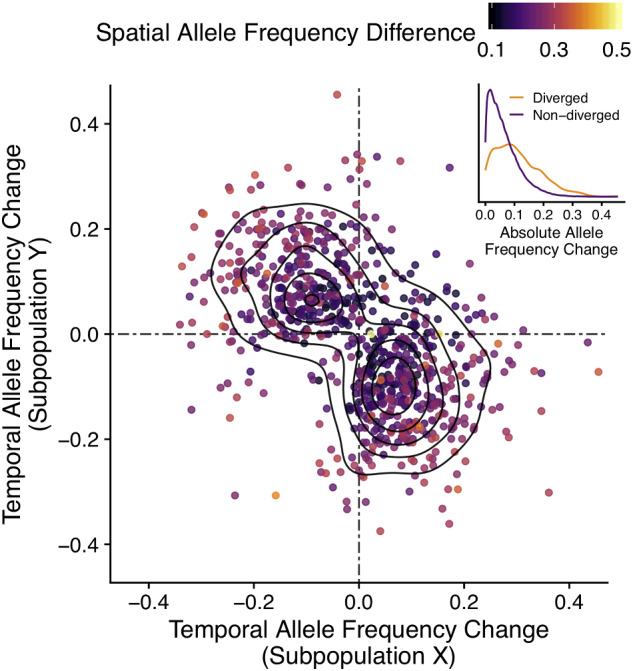
Within-generation allele frequency changes generate fine, spatial structure. Temporal allele frequency changes of 788 SNPs exhibiting significant spatial divergence in fall (geometric mean p < 0.01). x and y axes show the allele frequency change in two of the four subpopulations, with all six pairwise comparisons overlaid. Dashed lines mark the origin; solid contour lines the density distribution of SNPs. Coloration indicates the spatial allele frequency difference in fall. Inset shows the distribution of absolute allele frequency changes for non-diverged SNPs (purple) and for SNPs showing significant divergence in fall (orange).

Discussion

 

High site fidelity at small spatial scales (Lotrich 1975; Skinner et al. 2005, 2012; Able et al. 2012) combined with a large tag and recapture effort allowed for in situin situ monitoring of selective processes in this F. heteroclitus population. We find significant morphological differences among individuals inhabiting distinct niche environments (fig. 2). Although morphological divergence could be purely environment driven, that is, plastic, it is indicative of significant environmental differences among niches that could potentially be driving selection. For instance, the disparate temperature and dissolved oxygen regimes (Smith and Able 2003; Hunter et al. 2007) experienced by tidal pond and coastal basin residents are plausible drivers of selection given their direct effect on fitness related life history traits in ectotherms (Huey and Berrigan 2001; Stierhoff et al. 2003; Hunter et al. 2007; Kingsolver and Huey 2008; Dibble and Meyerson 2012; Hochachka and Somero 2014; Flatt 2020). Minimal spatial structure (supplementary fig. S5, Supplementary Material online) resulting from synchronous breeding in a common location provides a homogeneous genetic baseline upon which selection may act in any single environmental niche. In fact, GBS data of larval fish, caught throughout the estuary 2–4 weeks postspawning, do not show any population structure nor increased kinship among larvae caught at the same location (unpublished).

Within a single generation we find an elevated number of significant allele frequency changes that are unlikely caused by random mortality, sampling effects, linkage, or other neutral processes alone (fig. 4). In addition, we find an unexpectedly high proportion of allele frequency changes to be concordant among subpopulations in both magnitude and direction (fig. 5). Spatial data corroborate previous findings by Wagner et al. (2017), showing an elevated number of significantly differentiated SNPs among interbreeding, resident subpopulations within the same estuary (fig. 6). Finally, we show that spatially differentiated loci have undergone larger temporal allele frequency changes than undifferentiated loci (fig. 7). This suggest that fine spatial structure among niche subpopulations is primarily the result of within-generation allele frequency changes, not prior spatial structure.

Within-Generation, Local Adaptation by Polygenic Selection

Given its prolonged presence in New Jersey salt marshes (∼15,000 years) (Ropson et al. 1990), large effective population sizes on the order of 10⁴–10⁵ (Valiela et al. 1977; Duvernell et al. 2008), and a short generation time of 1 year (Kneib and Stiven 1978), one might expect F. heteroclitus to have successfully adapted to its habitat and reached equilibrium. Instead, we find an unexpectedly high number of minor allele frequency changes that shape spatial divergence among subpopulations, suggestive of local adaptation to niche environments. These observations are hard to reconcile, especially when selection is strong enough to produce detectable allele frequency changes within a single generation.

Polygenic selection leading to fine scale adaptation to niche environments offers a plausible explanation for the observed patterns. Given sufficient standing genetic variation and moderate redundancy in the alleles underlying a polygenic, fitness-related trait, subpopulations could potentially respond to niche-specific selection every generation following panmictic breeding (Goldstein and Holsinger 1992; Yeaman 2015). Assuming numerous combinations of redundant alleles can equally confer higher fitness, local adaptation is readily achieved with just minor allele frequency changes at multiple loci of small effect (Latta 1998; Le Corre and Kremer 2003, 2012). This makes quantitative traits with redundant, polygenic architectures and high levels of genetic variance the most likely candidates for this type of within-generation selection (Houle 1992; Yeaman 2015). In fact, several higher-order, fitness-related traits have been shown to be under redundant, polygenic control (Boyle et al. 2017; Zhang et al. 2018; Barghi et al. 2019; Flatt 2020).

Repeated, within-generation selection can be viewed as a particular case of local adaptation that does not result in evolutionary change across generations. However, it still generates subtle phenotypic divergence among niche residents that raises the niche-specific fitness of each subpopulation. In a heterogeneous landscape, within-generation selection may then create microgeographic patterns of local adaptation that are continuously generated and eroded (Richardson et al. 2014). Such genetic and phenotypic patterning at both short temporal and small spatial scales may then not only be of evolutionary interest but also have far-reaching ecological consequences (Hairston et al. 2005; Urban et al. 2020).

An essential requirement of adaptation via polygenic selection is high standing genetic variation which is however rapidly depleted by successive bouts of selection (Yeaman 2015; Jain and Stephan 2017). Sustained within-generation selection therefore requires genetic variance to be maintained across generations. However, the mechanisms underlying the maintenance of genetic variance remain poorly understood, especially in the case of polygenic traits with a redundant architecture. Nevertheless, several factors may facilitate the maintenance of polymorphism in F. heteroclitus. For instance, spatially heterogeneous environments have been shown to promote and maintain high standing genetic variation (Gillespie 1974; Gulisija and Kim 2015; Svardal et al. 2015). Density-dependent, soft selection (Wallace 1975) in resource-limited patches, such as the tidal ponds inhabited by F. heteroclitus (Kneib 1993; Hunter et al. 2007, 2009; Dibble and Meyerson 2012), has been shown to maintain polymorphism experimentally (Gallet et al. 2018).

Likewise, temporally heterogeneous environments can also maintain polymorphism in a population (Gillespie 1973; Bergland et al. 2014; Svardal et al. 2015; Wittmann et al. 2017; Bertram and Masel 2019). Fluctuations in biotic or abiotic factors, such as predator abundance or temperature (Yoshida et al. 2003; Paccard et al. 2018), can result in cyclic selection pressures that restrict fixation of temporarily beneficial alleles (Bergland et al. 2014; Gulisija and Kim 2015; Bertram and Masel 2019). In addition, age-dependent selection and overlapping generations can further stabilize polymorphism via the storage effect (Ellner and Hairston 1994; Gulisija and Kim 2015). For example, if selection predominantly occurs during the larval stage as it does for most teleosts like F. heteroclitus (Kneib and Stiven 1978; Kneib 1993), adult fish may “store” momentarily deleterious alleles until the environment reverts to conditions under which these become beneficial again. Stored alleles can then rise in frequency, possibly explaining the concordant, ecosystem-wide allele frequency changes observed here.

Finally, a continuous supply of new mutations is likely to be critical for sustained selection on standing genetic variation. Fortunately, this is discernibly higher for redundant, polygenic traits due to their larger mutational target, that is, the number of loci at which a new mutation will have an effect (Yeaman 2015; Hermisson and Pennings 2017; Höllinger et al. 2019). In addition, its large effective population size (Valiela et al. 1977; Duvernell et al. 2008) allows F. heteroclitus to attain one of the highest nucleotide diversities among vertebrates of 1.6% (Reid et al. 2016). Such genetic diversity, demonstrative of an elevated population-scaled mutation rate, may form the required basis for repeated within-generation local adaptation in F. heteroclitus.

Genetic Divergence among Replicate Niches

We did not observe a clear signal of pond subpopulations diverging in parallel from the basin subpopulation. Although significantly elevated, concordance among the three ponds is not higher than among any other three-way combination that includes the Basin, for example, Basin:Pond 1:Pond 3. Nevertheless, we observe within-generation allele frequency changes that result in an unexpected number of significantly differentiated loci among resident subpopulations, regardless of niche type. This result, previously demonstrated by Wagner et al. (2017), suggests environmental heterogeneity does not present as discrete partitioning into binary pond/basin niche types, but rather as a continuum of multiple, possibly obscure, environmental factors. Stuart et al. (2017) have shown that cryptic environmental differences among lake and stream habitats can explain the apparent lack of parallelism among paired stickleback populations. Likewise, cryptic environmental variables among ponds may be of similar, or higher, importance as the documented temperature and dissolved oxygen differences to the basin. For example, Hunter et al. (2007, 2009) demonstrated that tidal pond flooding frequency is positively correlated with female F. heteroclitus gonadosomatic index. The authors suggest that increased nutrient availability, introduced by frequent tidal flooding, may allow for higher reproductive allocation, a key life history and fitness-related trait. Hence, quasi-isolated, resident subpopulations are likely exposed to a multidimensional, heterogeneous fitness landscape with distinct selection pressures resulting in unique pheno- and genotypic responses.

An alternative explanation for the relative lack of parallelism among ponds is redundancy in the genetic architecture of traits under selection (Yeaman et al. 2018; Láruson et al. 2020). If distinct combinations of redundant alleles can induce the same phenotype, then replicate populations experiencing similar selection pressures may not necessarily share the same adaptive alleles (Fraser et al. 2015; Barghi et al. 2019). Under redundant, polygenic selection pond subpopulations may therefore show parallel, phenotypic divergence from the basin without exhibiting molecular parallelism. In fact, this mode of selection would present as mild divergence at redundant, adaptive loci among replicate niches as was observed here. Which loci ultimately effect an adaptive trait shift in any given niche may then simply depend on stochastic effects (Hermisson and Pennings 2017; Höllinger et al. 2019). For example, random dispersal of larvae across the estuary generates mild heterogeneity in standing genetic variation among ponds. Assuming similar effect sizes among redundant alleles, those at intermediate frequencies will be more responsive to selection (Hermisson and Pennings 2005; Barrett and Schluter 2008), resulting in unique adaptive outcomes within each pond. Nevertheless, distinguishing genetic redundancy from cryptic environmental differences among replicate niches is complex, especially in an uncontrolled, natural setting.

Matching Habitat Choice

The majority of F. heteroclitus exhibit limited dispersal (>60% stay within 20 m over several months), yet a significant proportion readily travels between niches during spring tides when the estuary floods (Skinner et al. 2005, 2012; Able et al. 2012). During early summer, monthly pond emigration rates can reach 30% compared with mortality rates of 20% (Hunter et al. 2009). Similar migration rates have also been reported in the basin, suggesting niches are in fact highly connected (Able et al. 2012). Here, the absence of tagged individuals in fall may therefore be due to either mortality or emigration. Although only a small proportion of tagged individuals migrated among sampling sites (4.6%), we cannot exclude the possibility of emigration into unsampled locations. Hence, the significant temporal allele frequency changes and resulting spatial structure observed here can be both the consequence of selection and/or non-random, genotype-dependent emigration. Note that immigration cannot have caused the observed allele frequency changes because immigrant fish, which carried either no tag or a “foreign” tag, were excluded from the analysis.

Genotype-dependent migration, or matching habitat choice, describes the process of organisms sensing their surroundings and actively seeking environments in which their fitness is maximized (Edelaar and Bolnick 2012; Nicolaus and Edelaar 2018). This can lead to adaptive, genetic divergence even when migration rates are prohibitively high for local adaptation under migration-selection balance (Edelaar and Bolnick 2012; Richardson et al. 2014). Further, matching habitat choice significantly reduces genetic load in outbred populations and can allow for the maintenance of standing genetic variation because alleles are not removed by selection but rather redistributed in space (Nicolaus and Edelaar 2018). Although several studies have demonstrated matching habitat choice in the wild (Jones and Probert 1980; Bolnick et al. 2009; Karpestam et al. 2012), it is a costlier strategy than evolving locally adapted genotypes or phenotypic plasticity (Nicolaus and Edelaar 2018). In fact, matching habitat choice is only favorable in 1) an actively dispersing species (Jacob et al. 2015) that 2) breeds panmictically, where 3) offspring distribute randomly throughout a habitat that is 4) highly heterogeneous both in space and time yet 5) offers minimal barriers to dispersal (Nicolaus and Edelaar 2018). Fundulus heteroclitus inhabiting New Jersey salt marshes evidently meet these criteria, making matching habitat choice a plausible, alternative explanation for the observed within-generation allele frequency changes.

Linkage Disequilibrium

The GBS approach only allowed for querying ∼0.3% of the ∼1 Gb F. heteroclitus genome. It is therefore plausible that large allele frequency changes in unsequenced regions of the genome were not identified. Hence, we cannot exclude the possibility that within-generation selection in F. heteroclitus is driven by large-effect loci. Linkage to unobserved loci under strong selection could also lead to an elevated number of minor, yet significant, allele frequency changes via “hitchhiking” (Barton 2000; Maynard Smith and Haigh 2007). Still, although we cannot exclude the presence of large-effect loci, it is unlikely that our observations are the result of hitchhiking alone. First, LD decays rapidly (within ∼500 bp, supplementary fig. S2, Supplementary Material online), indicating that the F. heteroclitus population is large and outbred. As a result, the extent of hitchhiking is reduced and the size of genomic islands around potential loci under strong selection are small (Barton 2000). The likelihood that the small proportion of loci assayed via GBS happen to be in linkage with and hitchhiking alongside unobserved, large-effect loci is therefore low. Second, if the elevated number of significant allele frequency changes would be caused by hitchhiking alone, significant SNPs should cluster around loci under strong selection. Instead, we find both loci with significant temporal allele frequency changes as well as significant spatial differentiation are evenly distributed throughout the genome (supplementary fig. S8, Supplementary Material online). Finally, the number of significant SNPs per scaffold is highly correlated to its length (Pearson’s r = 0.75, p ≪ 0.05) (supplementary fig. S9, Supplementary Material online), further supporting the conclusion that allele frequency changes are pervasive and evenly distributed, a pattern typical of polygenic architectures (Visscher et al. 2006).

Although linkage to unsampled, large-effect loci cannot explain our observations, linkage among the assayed loci could potentially be influencing our results. Within local recombination “cold spots,” for instance, tight linkage can inflate the observed number of significant loci relative to the expectation, leading to an overestimated O:E ratio. We reduced this bias by pruning the SNP set to only include loci separated by at least 300 bp which, in this naturally outbred population, significantly reduces mean linkage among loci (supplementary fig. S2, Supplementary Material online). Although our pruning approach does not exclude more distant linkage interactions, the results suggest that it sufficiently controls for linkage bias. Specifically, the permutation approach implicitly accounted for linkage because individuals rather than specific SNPs were permuted. p values generated by the permutations are highly correlated and near identical to those resulting from the simulation analyses and Barnard’s tests (supplementary fig. S3, Supplementary Material online). If results were primarily driven by linkage bias, permutation analyses would detect markedly fewer significant loci than the methods assuming independence among loci. Since this is not the case, linkage among assayed loci is unlikely to have caused elevated O:E ratios and within-generation, polygenic selection at multiple loci of small effect remains the most plausible explanation.

Conclusion and Future Directions

We have discovered significant, concordant allele frequency changes within a single generation among independent subpopulations of a well-mixed, larger population. Although only few loci are individually significant, we find an excess of allele frequency changes that are unexpected in a finite, closed population evolving under neutrality. Further, these allele frequency changes generate subtle, yet significant, divergence among subpopulations, suggestive of fine scale, local adaptation to distinct niche environments within a single generation. Although we cannot distinguish between selection and genotype-dependent emigration as drivers of significant allele frequency changes, the underlying genetic architecture seems to be polygenic. That is, the unknown trait involved in trait-dependent mortality (selection) and/or trait-dependent emigration likely has a polygenic basis. Although some ambiguities remain, redundant, polygenic selection, and/or trait-dependent emigration offer conceivable mechanisms for within-generation, local adaptation and polymorphism maintenance in the F. heteroclitus system.

Still, further work is necessary to validate this interpretation. First, comprehensive phenotyping of individuals is required to confirm selection and/or trait-dependent emigration effects a shift in trait means among niche residents. Given the stark differences both in temperature and dissolved oxygen between pond and basin habitats (Smith and Able 2003), traits known to be impacted by these abiotic factors are the most promising targets (Huey and Berrigan 2001; Stierhoff et al. 2003; Hunter et al. 2007; Kingsolver and Huey 2008; Dibble and Meyerson 2012; Hochachka and Somero 2014; Flatt 2020). In addition, differential survivorship in caged, reciprocal transplants of basin and pond residents could confirm selection on niche conditions and eliminate matching habitat choice as a potential mechanism.

Comprehensive whole-genome sequencing is required to determine the effect size distribution and confirm that polygenic architectures govern within-generation niche adaptation. A repeat of this experimental design would allow for assessing the consistency of allele frequency changes between generations and give a measure of genetic redundancy (Yeaman et al. 2018; Láruson et al. 2020). Finally, by combining phenotypic and genetic data, associations can be drawn between niche-specific allele frequency changes and the phenotypes under selection.

Detecting subtle signatures of redundant, polygenic selection on complex traits remains elusive. We acknowledge the limitations of the data presented here but encourage further work addressing repeated within-generation, polygenic selection not only in a laboratory setting but also in natural populations.

Ethics Statement

Fieldwork was completed within publicly available lands, and no permission was required for access. Fundulus heteroclitus does not have endangered or protected status, and small marine minnows do not require collection permits for noncommercial purposes. Adult F. heteroclitus was captured in minnow traps with minimal stress and removed in <1 h. Tag and recapture and nonsurgical tissue sampling protocols were in compliance with and approved by the University of Miami Institutional Animal Care and Use Committee (IACUC, protocols 16-124 and 19-119).

Supplementary Material

Supplementary data are available at Genome Biology and Evolution online.

Literature Cited

- Able KW. 1984. Variation in spawning site selection of the mummichog, Fundulus heteroclitus. Copeia 1984(2):522. [Google Scholar]
- Able KW, Felley JD. 1986. Geographical variation in Fundulus heteroclitus: tests for concordance between egg and adult morphologies. Am Zool. 26(1):145–157. [Google Scholar]
- Able KW, Vivian DN, Petruzzelli G, Hagan SM. 2012. Connectivity among salt marsh subhabitats: residency and movements of the mummichog (Fundulus heteroclitus). Estuaries Coasts. 35(3):743–753. [Google Scholar]
- Barghi N, et al. 2019. Genetic redundancy fuels polygenic adaptation in Drosophila. PLoS Biol. 17(2):e3000128. [DOI] [PMC free article] [PubMed] [Google Scholar]
- Barrett RDH, et al. 2019. Linking a mutation to survival in wild mice. Science 363(6426):499–504. [DOI] [PubMed] [Google Scholar]
- Barrett RDH, Schluter D. 2008. Adaptation from standing genetic variation. Trends Ecol Evol. 23(1):38–44. [DOI] [PubMed] [Google Scholar]
- Barton N, Hermisson J, Nordborg M. 2019. Why structure matters: great care is needed when interpreting claims about the genetic basis of human variation based on data from genome-wide association studies. Elife 8. doi: 10.7554/eLife.45380. [Google Scholar]
- Barton NH. 2000. Genetic hitchhiking. Philos Trans R Soc Lond B. 355(1403):1553–1562. [DOI] [PMC free article] [PubMed] [Google Scholar]
- Barton NH, Etheridge AM. 2018. Establishment in a new habitat by polygenic adaptation. Theor Popul Biol. 122:110–127. [DOI] [PubMed] [Google Scholar]
- Barton NH, Etheridge AM, Véber A. 2017. The infinitesimal model: definition, derivation, and implications. Theor Popul Biol. 118:50–73. [DOI] [PubMed] [Google Scholar]
- Beaumont MA, Nichols RA. 1996. Evaluating loci for use in the genetic analysis of population structure. Proc R Soc B Biol Sci. 263:1619–1626. [Google Scholar]
- Berg JJ, et al. 2019. Reduced signal for polygenic adaptation of height in UK Biobank. Elife. 8. doi: 10.7554/eLife.39725. [DOI] [PMC free article] [PubMed] [Google Scholar]
- Berg JJ, Coop G. 2014. A population genetic signal of polygenic adaptation. PLoS Genet. 10(8):e1004412. [DOI] [PMC free article] [PubMed] [Google Scholar]
- Bergland AO, Behrman EL, O’Brien KR, Schmidt PS, Petrov DA. 2014. Genomic evidence of rapid and stable adaptive oscillations over seasonal time scales in Drosophila. PLoS Genet. 10(11):e1004775. [DOI] [PMC free article] [PubMed] [Google Scholar]
- Bertram J, Masel J. 2019. Different mechanisms drive the maintenance of polymorphism at loci subject to strong versus weak fluctuating selection. Evolution (N. Y.) 73(5):883–896. [DOI] [PubMed] [Google Scholar]
- Bolnick DI, et al. 2009. Phenotype-dependent native habitat preference facilitates divergence between parapatric lake and stream stickleback. Evolution (N. Y.) 63(8):2004–2016. [DOI] [PubMed] [Google Scholar]
- Boyle EA, Li YI, Pritchard JK. 2017. An expanded view of complex traits: from polygenic to omnigenic. Cell 169(7):1177–1186. [DOI] [PMC free article] [PubMed] [Google Scholar]
- Dayan DI, et al. 2019. Population genomics of rapid evolution in natural populations: polygenic selection in response to power station thermal effluents. BMC Evol Biol. 19:1–20. [DOI] [PMC free article] [PubMed] [Google Scholar]
- Dibble KL, Meyerson LA. 2012. Tidal flushing restores the physiological condition of fish residing in degraded salt marshes. PLoS One 7(9):e46161. [DOI] [PMC free article] [PubMed] [Google Scholar]
- Duvernell DD, Lindmeier JB, Faust KE, Whitehead A. 2008. Relative influences of historical and contemporary forces shaping the distribution of genetic variation in the Atlantic killifish, Fundulus heteroclitus. Mol Ecol. 17(5):1344–1360. [DOI] [PubMed] [Google Scholar]
- Edelaar P, Bolnick DI. 2012. Non-random gene flow: an underappreciated force in evolution and ecology. Trends Ecol Evol. 27(12):659–665. [DOI] [PubMed] [Google Scholar]
- Ellner S, Hairston NG. 1994. Role of overlapping generations in maintaining genetic variation in a fluctuating environment. Am Nat. 143(3):403–417. [Google Scholar]
- Elshire RJ, et al. 2011. A robust, simple genotyping-by-sequencing (GBS) approach for high diversity species. PLoS One 6(5):e19379-10. [DOI] [PMC free article] [PubMed] [Google Scholar]
- Flatt T. 2020. Life-history evolution and the genetics of fitness components in Drosophila melanogaster. Genetics 214(1):3–48. [DOI] [PMC free article] [PubMed] [Google Scholar]
- Fraser BA, Künstner A, Reznick DN, Dreyer C, Weigel D. 2015. Population genomics of natural and experimental populations of guppies (Poecilia reticulata). Mol Ecol. 24(2):389–408. [DOI] [PubMed] [Google Scholar]
- Gallet R, Froissart R, Ravigné V. 2018. Experimental demonstration of the impact of hard and soft selection regimes on polymorphism maintenance in spatially heterogeneous environments. Evolution (N. Y.) 72(8):1677–1688. [DOI] [PubMed] [Google Scholar]
- Gillespie J. 1973. Polymorphism in random environments. Theor Popul Biol. 4(2):193–195. [Google Scholar]
- Gillespie J. 1974. Polymorphism in patchy environments. Am Nat. 108(960):145–151. [Google Scholar]
- Goldstein DB, Holsinger KE. 1992. Maintenance of polygenic variation in spatially structured populations: roles for local mating and genetic redundancy. Evolution (N. Y.) 46(2):412. [DOI] [PubMed] [Google Scholar]
- Gompert Z, et al. 2014. Experimental evidence for ecological selection on genome variation in the wild. Ecol Lett. 17(3):369–379. [DOI] [PMC free article] [PubMed] [Google Scholar]
- Gulisija D, Kim Y. 2015. Emergence of long-term balanced polymorphism under cyclic selection of spatially variable magnitude. Evolution (NY) 69(4):979–992. [DOI] [PubMed] [Google Scholar]
- Hairston NG, Ellner SP, Geber MA, Yoshida T, Fox JA. 2005. Rapid evolution and the convergence of ecological and evolutionary time. Ecol. Lett. 8(10):1114–1127. [Google Scholar]
- Haldane JBS. 1957. The cost of natural selection. J Genet. 55(3):511–524. [Google Scholar]
- Harris RB, Sackman A, Jensen JD. 2018. On the unfounded enthusiasm for soft selective sweeps II: examining recent evidence from humans, flies, and viruses. PLoS Genet. 14(12):e1007859-21. [DOI] [PMC free article] [PubMed] [Google Scholar]
- Hendry AP, Nosil P, Rieseberg LH. 2007. The speed of ecological speciation. Funct Ecol. 21(3):455–464. [DOI] [PMC free article] [PubMed] [Google Scholar]
- Hermisson J, Pennings PS. 2005. Soft sweeps: molecular population genetics of adaptation from standing genetic variation. Genetics 169(4):2335–2352. [DOI] [PMC free article] [PubMed] [Google Scholar]
- Hermisson J, Pennings PS. 2017. Soft sweeps and beyond: understanding the patterns and probabilities of selection footprints under rapid adaptation. Methods Ecol Evol. 8(6):700–716. [Google Scholar]
- Hochachka PW, Somero GN. 2014. Biochemical adaptation. Princeton (NJ): Princeton University Press. [Google Scholar]
- Höllinger I, Pennings PS, Hermisson J. 2019. Polygenic adaptation: from sweeps to subtle frequency shifts. PLoS Genet. 15(3):e1008035. [DOI] [PMC free article] [PubMed] [Google Scholar]
- Houle D. 1992. Comparing evolvability and variability of quantitative traits. Genetics 130(1):195–204. [DOI] [PMC free article] [PubMed] [Google Scholar]
- Huey RB, Berrigan D. 2001. Temperature, demography, and ectotherm fitness. Am Nat. 158(2):204–210. [DOI] [PubMed] [Google Scholar]
- Hunter KL, Fox MG, Able KW. 2007. Habitat influences on reproductive allocation and growth of the mummichog (Fundulus heteroclitus) in a coastal salt marsh. Mar Biol. 151(2):617–627. [Google Scholar]
- Hunter KL, Fox MG, Able KW. 2009. Influence of flood frequency, temperature and population density on migration of Fundulus heteroclitus in semi-isolated marsh pond habitats. Mar Ecol Prog Ser. 391:85–96. [Google Scholar]
- Jacob S, Bestion E, Legrand D, Clobert J, Cote J. 2015. Habitat matching and spatial heterogeneity of phenotypes: implications for metapopulation and metacommunity functioning. Evol Ecol. 29(6):851–871. [Google Scholar]
- Jain K, Stephan W. 2017. Modes of rapid polygenic adaptation. Mol Biol Evol. 34(12):3169–3175. [DOI] [PubMed] [Google Scholar]
- Jensen JD, et al. 2019. The importance of the neutral theory in 1968 and 50 years on: a response to Kern and Hahn 2018. Evolution (N. Y.) 73(1):111–114. [DOI] [PMC free article] [PubMed] [Google Scholar]
- Johri P, Charlesworth B, Jensen JD. 2020. Toward an evolutionarily appropriate null model: jointly inferring demography and purifying selection. Genetics 215(1):173–192. [DOI] [PMC free article] [PubMed] [Google Scholar]
- Jones JS, Probert RF. 1980. Habitat selection maintains a deleterious allele in a heterogeneous environment. Nature 287(5783):632–633. [Google Scholar]
- Karpestam E, Wennersten L, Forsman A. 2012. Matching habitat choice by experimentally mismatched phenotypes. Evol Ecol. 26(4):893–907. [Google Scholar]
- Kern AD, Hahn MW. 2018. The neutral theory in light of natural selection. Mol Biol Evol. 35(6):1366–1371. [DOI] [PMC free article] [PubMed] [Google Scholar]
- Kimball ME, Able KW. 2012. Tidal migrations of intertidal salt marsh creek nekton examined with underwater video. Northeast Nat. 19(3):475–486. [Google Scholar]
- Kimura M. 1968. Evolutionary rate at the molecular level. Nature 217(5129):624–626. [DOI] [PubMed] [Google Scholar]
- Kingsolver JG, Huey RB. 2008. Size, temperature, and fitness: three rules. Evol Ecol Res. 10:251–268. [Google Scholar]
- Kneib RT. 1993. Growth and mortality in successive cohorts of fish larvae within an estuarine nursery. Mar Ecol Prog Ser. 94:115–127. [Google Scholar]
- Kneib RT, Stiven A. 1978. Growth, reproduction, and feeding of Fundulus heteroclitus(L.) on a North Carolina salt marsh. J Exp Mar Biol Ecol. 31(2):121–140. [Google Scholar]
- Kreitman M. 1996. The neutral theory is dead. Long live the neutral theory. Bioessays 18(8):678–683. [DOI] [PubMed] [Google Scholar]
- Láruson ÁJ, Yeaman S, Lotterhos KE. 2020. The importance of genetic redundancy in evolution. Trends Ecol Evol. 35(9):809–822. [DOI] [PubMed] [Google Scholar]
- Latta RG. 1998. Differentiation of allelic frequencies at quantitative trait loci affecting locally adaptive traits. Am Nat. 151(3):283–292. [DOI] [PubMed] [Google Scholar]
- Le Corre V, Kremer A. 2003. Genetic variability at neutral markers, quantitative trait loci and trait in a subdivided population under selection. Genetics 164:1205–1219. [DOI] [PMC free article] [PubMed] [Google Scholar]
- Le Corre V, Kremer A. 2012. The genetic differentiation at quantitative trait loci under local adaptation. Mol Ecol. 21(7):1548–1566. [DOI] [PubMed] [Google Scholar]
- Lewontin RC. 1974. The paradox of variation In: Ridley M, editor. The genetic basis of evolutionary change. Oxford (UK): Oxford University Press, p. 189–271. [Google Scholar]
- Lotrich VA. 1975. Summer home range and movements of Fundulus Heteroclitus (Pisces: Cyprinodontidae) in a Tidal Creek. Ecology 56(1):191–198. [Google Scholar]
- Maynard Smith J, Haigh J. 2007. The hitch-hiking effect of a favourable gene. Genet Res. 89(5–6):391–403. [DOI] [PubMed] [Google Scholar]
- Messer PW, Ellner SP, Hairston NG. 2016. Can population genetics adapt to rapid evolution? Trends Genet. 32(7):408–418. [DOI] [PubMed] [Google Scholar]
- Nicolaus M, Edelaar P. 2018. Comparing the consequences of natural selection, adaptive phenotypic plasticity, and matching habitat choice for phenotype–environment matching, population genetic structure, and reproductive isolation in meta-populations. Ecol Evol. 8(8):3815–3827. [DOI] [PMC free article] [PubMed] [Google Scholar]
- Nowak MA, Boerlijst MC, Cooke J, Smith JM. 1997. Evolution of genetic redundancy. Nature 388(6638):167–170. [DOI] [PubMed] [Google Scholar]
- Orr HA. 2005. The genetic theory of adaptation: a brief history. Nat Rev Genet. 6(2):119–127. [DOI] [PubMed] [Google Scholar]
- Paccard A, et al. 2018. Adaptation in temporally variable environments: stickleback armor in periodically breaching bar-built estuaries. J Evol Biol. 31(5):735–752. [DOI] [PubMed] [Google Scholar]
- Pritchard JK, Di Rienzo A. 2010. Adaptation—not by sweeps alone. Nat Rev Genet. 11(10):665–667. [DOI] [PMC free article] [PubMed] [Google Scholar]
- Pritchard JK, Pickrell JK, Coop G. 2010. The genetics of human adaptation: hard sweeps, soft sweeps, and polygenic adaptation. Curr Biol. 20(4):R208–R215. [DOI] [PMC free article] [PubMed] [Google Scholar]
- Przeworski M, Coop G, Wall JD. 2005. The signature of positive selection on standing genetic variation. Evolution 59(11):2312–2323. [PubMed] [Google Scholar]
- Reid NM, et al. 2016. The genomic landscape of rapid repeated evolutionary adaptation to toxic pollution in wild fish. Science 354(6317):1305–1308. [DOI] [PMC free article] [PubMed] [Google Scholar]
- Richardson JL, Urban MC, Bolnick DI, Skelly DK. 2014. Microgeographic adaptation and the spatial scale of evolution. Trends Ecol Evol. 29(3):165–176. [DOI] [PubMed] [Google Scholar]
- Rockman MV. 2012. The QTN program and the alleles that matter for evolution: all that’s gold does not glitter. Evolution (N. Y.) 66(1):1–17. [DOI] [PMC free article] [PubMed] [Google Scholar]
- Ropson IJ, Brown DC, Powers DA. 1990. Biochemical genetics of Fundulus heteroclitus (L.). VI. Geographical variation in the gene frequencies of 15 loci. Evolution (N. Y.) 44(1):16. [DOI] [PubMed] [Google Scholar]
- Sella G, Barton NH. 2019. Thinking about the evolution of complex traits in the era of genome-wide association studies. Annu Rev Genomics Hum Genet. 20:461–493. [DOI] [PubMed] [Google Scholar]
- Skinner MA, Courtenay SC, Parker WR, Curry RA. 2005. Site fidelity of mummichogs (Fundulus heteroclitus) in an Atlantic Canadian Estuary. Water Qual Res J Canada. 40(3):288–298. [Google Scholar]
- Skinner MA, Courtenay SC, Parker WR, Curry RA. 2012. Stable isotopic assessment of site fidelity of mummichogs, Fundulus heteroclitus, exposed to multiple anthropogenic inputs. Environ Biol Fish. 94(4):695–706. [Google Scholar]
- Smith KJ, Able KW. 2003. Dissolved oxygen dynamics in salt marsh pools and its potential impacts on fish assemblages. Mar Ecol Prog Ser. 258:223–232. [Google Scholar]
- Sohail M, et al. 2019. Polygenic adaptation on height is overestimated due to uncorrected stratification in genome-wide association studies. Elife 8:e39702. [DOI] [PMC free article] [PubMed] [Google Scholar]
- Stierhoff KL, Targett TE, Grecay PA. 2003. Hypoxia tolerance of the mummichog: the role of access to the water surface. J Fish Biol. 63(3):580–592. [Google Scholar]
- Stuart YE, et al. 2014. Rapid evolution of a native species following invasion by a congener. Science 346(6208):463–466. [DOI] [PubMed] [Google Scholar]
- Stuart YE, et al. 2017. Contrasting effects of environment and genetics generate a continuum of parallel evolution. Nat Ecol Evol. 1:1–7. [DOI] [PubMed] [Google Scholar]
- Svardal H, Rueffler C, Hermisson J. 2015. A general condition for adaptive genetic polymorphism in temporally and spatially heterogeneous environments. Theor Popul Biol. 99:76–97. [DOI] [PubMed] [Google Scholar]
- Taylor MH, Leach GJ, DiMichele L, Levitan WM, Jacob WF. 1979. Lunar spawning cycle in the mummichog, Fundulus heteroclitus (Pisces: cyprinodontidae). Copeia. 1979(2):291. [Google Scholar]
- Urban MC, et al. 2020. Evolutionary origins for ecological patterns in space. Proc Natl Acad Sci U S A. 117(30):17482–17490. [DOI] [PMC free article] [PubMed] [Google Scholar]
- Valiela I, Wright JE, Teal JM, Volkmann SB. 1977. Growth, production and energy transformations in the salt-marsh killifish Fundulus heteroclitus. Mar Biol. 40(2):135–144. [Google Scholar]
- Visscher PM, et al. 2006. Assumption-free estimation of heritability from genome-wide identity-by-descent sharing between full siblings. PLoS Genet. 2(3):e41. [DOI] [PMC free article] [PubMed] [Google Scholar]
- Vovk V, Wang R. 2020. Combining p-values via averaging. Biometrika 107(4):791–808. [Google Scholar]
- Wagner DN, et al. 2017. Fine-scale genetic structure due to adaptive divergence among microhabitats. Heredity (Edinb) 118(6):594–604. [DOI] [PMC free article] [PubMed] [Google Scholar]
- Wallace B. 1975. Hard and soft selection revisited. Evolution (N. Y.) 29(3):465. [DOI] [PubMed] [Google Scholar]
- Whiting JR, Fraser BA. 2020. Contingent convergence: the ability to detect convergent genomic evolution is dependent on population size and migration. G3 Genes, Genomes, Genet 10:677–693. [DOI] [PMC free article] [PubMed] [Google Scholar]
- Wickland DP, Battu G, Hudson KA, Diers BW, Hudson ME. 2017. A comparison of genotyping-by-sequencing analysis methods on low-coverage crop datasets shows advantages of a new workflow, GB-eaSy. BMC Bioinformatics 18(1):1–12. [DOI] [PMC free article] [PubMed] [Google Scholar]
- Williams LM, Oleksiak MF. 2011. Ecologically and evolutionarily important SNPs identified in natural populations. Mol Biol Evol. 28(6):1817–1826. [DOI] [PMC free article] [PubMed] [Google Scholar]
- Wittmann MJ, Bergland AO, Feldman MW, Schmidt PS, Petrov DA. 2017. Seasonally fluctuating selection can maintain polymorphism at many loci via segregation lift. Proc Natl Acad Sci U S A. 114(46):E9932–E9941. [DOI] [PMC free article] [PubMed] [Google Scholar]
- Yeaman S. 2015. Local adaptation by alleles of small effect. Am Nat. 186(S1):S74–S89. [DOI] [PubMed] [Google Scholar]
- Yeaman S, Gerstein AC, Hodgins KA, Whitlock MC. 2018. Quantifying how constraints limit the diversity of viable routes to adaptation. PLoS Genet. 14(10):e1007717. [DOI] [PMC free article] [PubMed] [Google Scholar]
- Yoshida T, Jones LE, Ellner SP, Fussmann GF, Hairston NG. 2003. Rapid evolution drives ecological dynamics in a predator-prey system. Nature 424(6946):303–306. [DOI] [PubMed] [Google Scholar]
- Zhang Y, Qi G, Park JH, Chatterjee N. 2018. Estimation of complex effect-size distributions using summary-level statistics from genome-wide association studies across 32 complex traits. Nat Genet. 50(9):1318–1326. [DOI] [PubMed] [Google Scholar]
Associated Data
This section collects any data citations, data availability statements, or supplementary materials included in this article.
Supplementary Materials
Data Availability Statement
Raw and filtered variant sets as well as tag & recapture and morphological data are available on Dryad (doi:10.5061/dryad.0gb5mkm0c). Demultiplexed read data has been submitted to NCBI SRA under the BioProject ID: PRJNA688582.