Efficient neural spike sorting using data subdivision and unification

Abstract

Neural spike sorting is prerequisite to deciphering useful information from electrophysiological data recorded from the brain, in vitro and/or in vivo. Significant advancements in nanotechnology and nanofabrication has enabled neuroscientists and engineers to capture the electrophysiological activities of the brain at very high resolution, data rate and fidelity. However, the evolution in spike sorting algorithms to deal with the aforementioned technological advancement and capability to quantify higher density data sets is somewhat limited. Both supervised and unsupervised clustering algorithms do perform well when the data to quantify is small, however, their efficiency degrades with the increase in the data size in terms of processing time and quality of spike clusters being formed. This makes neural spike sorting an inefficient process to deal with large and dense electrophysiological data recorded from brain. The presented work aims to address this challenge by providing a novel data pre-processing framework, which can enhance the efficiency of the conventional spike sorting algorithms significantly. The proposed framework is validated by applying on ten widely used algorithms and six large feature sets. Feature sets are calculated by employing PCA and Haar wavelet features on three widely adopted large electrophysiological datasets for consistency during the clustering process. A MATLAB software of the proposed mechanism is also developed and provided to assist the researchers, active in this domain.

Introduction

Neuro-engineering is an interdisciplinary research domain that provides a collaborative platform for engineers, scientists, neurologists and clinicians to grow a robust and reliable communication network between human brain and computers using advanced engineering procedures, methods, tools and algorithms [1–3]. It is largely accepted hypothesis that the brain passes information in terms of neurons’ firings i.e. action potential or spikes over specific interval of time, known as neuron firing rate. Neurophysiological study of these hefty action potentials or spikes emanating from the neural network of the brain is essential to reveal the underlying behaviours and properties of neurons. A good understanding of the human brain neuronal network or nervous system is critically important in developing brain machine interfaces (BMIs), neuro-prosthetics and comprehensive brain-computer communication networks [4].

Electrophysiological analysis has attracted paramount importance, in recent years, in deciphering useful information about the underlying functional behaviour of the brain both in spontaneous and stimulated environments [5, 6]. This has paved the way of new discoveries in understanding the impact of external stimuli such as pharmaceuticals [7] and infections on the brain functionality [8]. Researchers have successfully developed the neural decoders from the neurophysiological study of intra neural recordings of human primary motor cortex to drive the artificial prostheses [9]. Electrophysiological studies also find significant importance in treating patients having neurological diseases or mental disorders especially in the case of epileptic disease. In addition, these studies have played vital role in understanding the gamma-protocadherine influences in regulating the neural network endurance and generating new neural synapses [10].

The significance of electrophysiological study of human brain lies in intercepting the neuronal signals with negligible interference in brain’s natural functionality. Numerous electrophysiological methods are found in the literature to monitor the action potentials or spikes from neurons, such as intracellular glass pipette electrodes [11], patch clamp electrodes [12, 13], extracellular single or multi-site electrodes [14], and optical imaging devices [15, 16]. Among all, extracellular recordings using micro fabricated electrode arrays [17–19] are largely preferable in research because of its relatively less impact on the normal working behaviour of neurons [20]. Extracellular recordings are further categorised into invasive (in-vivo) and non-invasive (in-vitro) approaches [21]. In in-vivo approach, microelectrodes such as a probe or tetrode (probe with four electrodes) is surgically implanted in the understudy region of the brain. Whereas, in in-vitro approach, neurons are cultured on the separate dishes integrated with microelectrodes [22]. The neurophysiological technology implemented to record neural action potentials is very advanced, but still it is very immature to record the action potentials emanating from a single neuron. Brain consists of closely packed neurons that mostly excites simultaneously to encode information consisting of synchronised and correlated action potentials [23, 24]. Neurons present in the surrounding or neighbourhood of the understudy region, when excited, introduce noise in the neural recordings [25, 26]. Therefore, to study and analyse the behaviour of individual neurons and to group the action potentials having similar features into specific clusters, the concept of ‘Spike Sorting’ is implemented [27, 28].

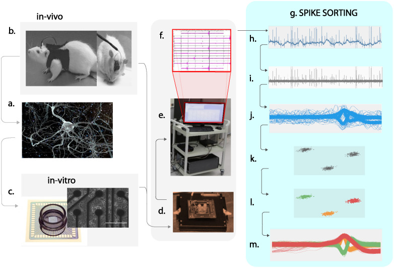
An overview of in-vivo and in-vitro recordings and complete description of the steps involved in the spike sorting process is illustrated in Fig 1. Spike sorting consists of four main steps. First, raw data is filtered to minimise the effect of noise. The work of Choi et al. in [29] has significance importance in reducing the effect of background noise and detecting useful spikes trains from neural recordings at low signal to noise ratio (SNR) using multi resolution Teager energy operator (MTEO). Paralikar et al. in [30] proposed the virtual referencing (VR) method based on average functional electrode signal and inter-electrode correlation (IEC) method based on correlation coefficient between threshold exceeding spikes segments for common noise reduction. Common noise is generally produced by electromyographic activity, motion artifacts, and electric field pickup, especially in awake/behaving subjects. Pillow et al. in [30] proposed binary pursuit algorithm to significantly reduce the effect of stochastic background component of correlated Gaussian noise from the neural recordings. Takekawa et. al in [31] worked on filtering the biological noise from the neural recording using peak band pass filtering technique. Band pass filtering is a common practice among neural scientists for reducing the effect of background noise. This followed by spike extraction [32]. Abeles and Golstein in [33], elaborated extensively about multi-unit spikes detection. Threshold and inter-spike interval based detection methods are frequent and popular among researchers [34]. However, in the proposed algorithm the focus is on the computation efficiency of spike sorting algorithms rather than the spike estimation. For the proposed research work, spikes are extracted using labels provided with the data to make comparison of performance between different algorithms unbiased due to noise effects. The third step in spike sorting is the feature extraction of detected spikes [35]. The latest feature extraction technique is proposed by Zamani and Demosthenous in [36], however, feature extraction techniques that are largely practised by researchers are Principal Component Analysis (PCA) [37–39], Wavelet Transform [40–42] and Wavelet Packet Decomposition [43]. The last step in this process is the clustering of spikes into specific action potential groups having similar features [44]. For clustering, scientists have proposed numerous clustering algorithms in the literature [45–48] that are mainly classified into two main categories; Supervised [49] and Un-Supervised [50]. In supervised clustering, the number of clusters are predefined and the algorithms forced the spikes to fit into desired number of predefined clusters [51]. Whereas, in unsupervised clustering, algorithms, without having prior clustering information, automatically estimate the total cluster numbers and based on similarity in spike features, label the spikes into their respective groups [52]. The unsupervised clustering is more reliable and useful when there is no prior knowledge about clusters [53]. The spike sorting algorithms are mainly used offline and are implemented for behavioural quantification on pre-recorded neural datasets [54]. However, researchers have developed online spike sorting algorithms that can quantify spike-clusters on live neural recordings [55]. The latest state of art in spike sorting process is presented in [56].

Fig 1. An overview of spike sorting process with in-vivo and in-vitro recordings.

(a) Microscopic image of neural network in the brain. (b) Brains cells cultured on the Micro-Electrode Arrays (MEAs). (c) Implanted probe in the rat brain for in vivo recordings. (d) Data acquisition system to interface with MEAs (e) Computing machine for data processing and spike sorting. (f) Multichannel data acquisition and recording (g) Visualisation of complete spike sorting process. (h) Raw data after sampling and amplification. (i) Noise filtering of data using band pass filters. (j) Spikes detected using the threshold or inter-spike interval methods. (k) Feature extraction of the detected spikes to reduce the dimensionality of the data. (l) Clustered features after applying clustering algorithms extracted spike features. (m) Clustered spikes.

Problem statement

Advancements in nanotechnology and nanofabrication has enabled neuroscientists and engineers to capture the electrophysiological activities of the brain at very high resolution, data rate and fidelity. However, to decipher useful information from these high dense electrode data, performance in terms of computational speed and accuracy of these spike-sorting algorithms, independent of their online and offline nature, plays an important role.

Stevenson and Kording in [57], presented data analysis issues due to progressive technological advancements of neural recordings. Progress in neural recording techniques enabling simultaneous multi channels recording is projected to double every 7 years resulting in high density and large size data. It is estimated that recording from 1000 neurons simultaneously could be achieved by 2025. The most recent automated spike sorting algorithm proposed by Chung et al. in [58] also highlighted the issue of low computational speed of spike sorting algorithms. Although they have proposed an efficient method for spike sorting, it lacks the speed researchers require for optimal results when sorting larger and high dense datasets. Wild et al. in [59] studied the performance evaluation on widely used clustering algorithms. His research outcomes highlighted the dependency of computational speed on data size or number of spikes to be clustered.

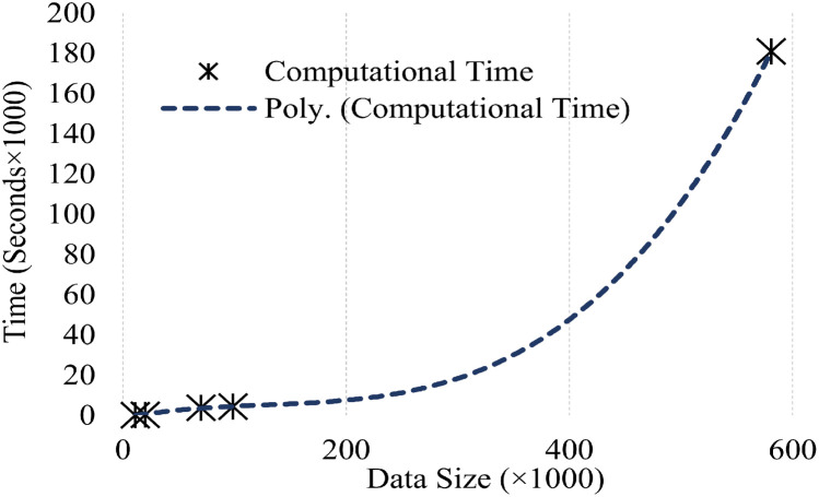
Chen and Cai in [60] investigated the issue and proposed that this behaviour is due to complexity of operations involved in the algorithms. They reported, for n size of data, spectral clustering requires O(n²) (second order equation) operations in graph construction and O(n³) (third order equation) operations in Eigen-decomposition. These second order and third order equations prove the non-linear behaviour of spectral clustering. To motivate our analysis, spectral clustering was applied on five datasets of variable length and calculated the corresponding computational time as in Table 1. The plot in Fig 2, clearly depicts the non-linear behaviour in computational time required by spectral clustering to complete its operations with respect to data size.

Table 1. Computational times of five datasets for spectral clustering.

Data Name	Data Size	# of classes	Computational Time
MNIST [61]	70000	10	3654.90
LetterRec [62]	20000	26	195.63
PenDigits [62]	10992	10	60.48
Seismic [63]	98528	3	4328.35
Covtype [62]	581012	7	181006.17

Fig 2. Computational time versus data size plot.

The dependency of speed and computational time on data size in spike-sorting has made it very difficult to efficiently and accurately identify the total number of neurons in large and dense electrophysiological data. Furthermore, based on the work of Napoleon and Pavalakodi on large, dense and high dimensional breast cancer cell data [64], the accuracy of clustering algorithms is also somehow contingent to the data size. With the increase in data size the occurrence of false positives and negatives in spike sorting increases significantly, which reduces the overall efficiency and performance of the algorithms involved in the process.

Despite these challenges, in literature, researchers have developed numerous spike sorting algorithms to address the challenge of handling large and dense electrophysiological data. However, limited work has considered enhancing computational speed and efficiency by changing the way we input data into spike sorting algorithms. The proposed algorithm pre-processes data to significantly reduce computational time and to enhance speed and efficiency of a wide range of existing spike sorting algorithms. The proposed algorithm has great potential to be adopted by parallel computing approaches to further enhance spike sorting algorithms’ efficiency for real-time online spike analysis.

Proposed mechanism

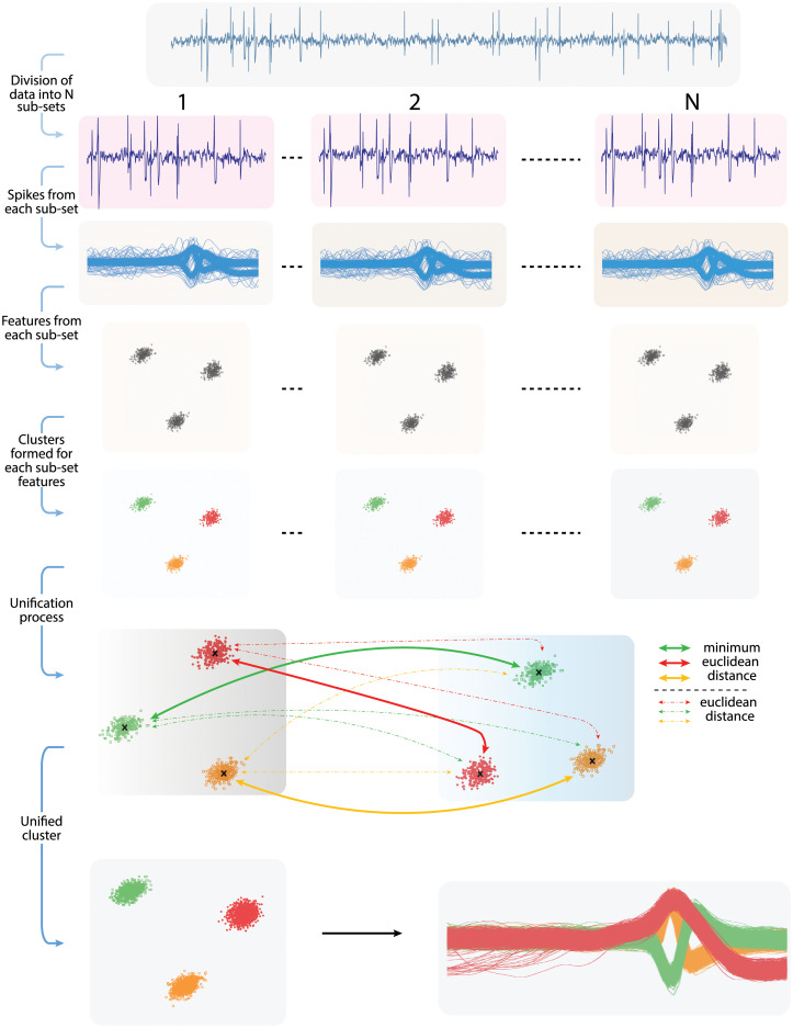
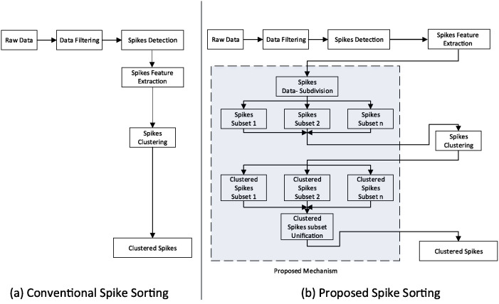
The novelty of the proposed mechanism lies in its capability to operate the existing spike sorting algorithms at their peak efficiency by introducing the optimal length subsets of large electrophysiological data at clustering stage. The overall mechanism consists of three major steps as illustrated in Fig 3. 1) The first step involves subdivision of data into data-subsets of optimal length. The procedure to identify optimal length is discussed in next section. 2) The second step involves clustering spikes in data-subsets using conventional spike sorting algorithms. 3) The last step involves unification of the clustered subsets. The final unified clusters are then used to label the detected spikes representing complete large electrophysiological data into their respective neural classes. The comparison of conventional spike sorting and proposed algorithm is depicted in Fig 4. It is worth mentioning that the proposed mechanism deals with data- subdivision and unification to felicitate and enhance the performance of existing clustering algorithms and does not modify the internal workings of the algorithms employed in this study. A recently developed clustering algorithm “Mountainsort” by Chung et al. [58] uses a density based approach to cluster spikes can also be used with this mechanism for efficient spike sorting.

Fig 3. Illustration of complete proposed mechanism.

The first step is to divide the large electrophysiological data into smaller groups. Second step involves the clustering of data-subsets using the conventional spike sorting algorithms. Last step involves the unification or merging of clustered data-subsets to get optimal clustering of complete large electrophysiological data.

Fig 4. Comparison of conventional and proposed spike sorting process.

A similar approach of data subdivision is used by Pachitariu et al. in [65] for KiloSort algorithm. The algorithm divides the high dense neural data into small batches and uses them for mean-time processing of data filtering in the GPU that reduces the overall time of the spike sorting process. However, clustering of spikes is still deployed at complete large neural datasets, which resulted into the slower computational speed of spike sorting at clustering stage. In addition, as opposed to proposed mechanism, the data-subdivision mechanism is limited to KiloSort and may not be applicable for other spike sorting algorithms. Furthermore, this algorithm failed to introduce the concept of optimal length for data-subdivision which is an important parameter to consider in enhancing the computational speed and operational cost of spike sorting process.

The detailed description of the steps involved in the proposed mechanism is provided in the following sections:

Data subdivision

Subdividing large electrophysiological data into optimal length subsets is the most critical component of proposed mechanism. To form data subsets, let D represents the electrophysiological data recorded at a single acquisition channel. The total number N of optimal subdivisions is estimated as in Eq (1)

$$\begin{array}{c}\hfill N=\frac{L}{O_L}\end{array}$$ (1)

where L is the length of data D and O_L is the optimal length for data-subsets. The procedure to calculate O_L is presented in the next section.

The data-subsets are then estimated as in Eq (2).

$$\begin{array}{c}\hfill S_d\left(n\right)=\left\{\begin{array}{c}D(1+(n-1)*N):D(n*N)n*N<D_t\\ D(1+(n-1):D(D_t)n*N\ge D_t\end{array}\right\}\\ \forall n=1,2,3,4\dots N\end{array}$$ (2)

where S_d(n) represents n number of subdivided data-subsets of the large data D.

Identification of optimal length (O_L) for data-subsets

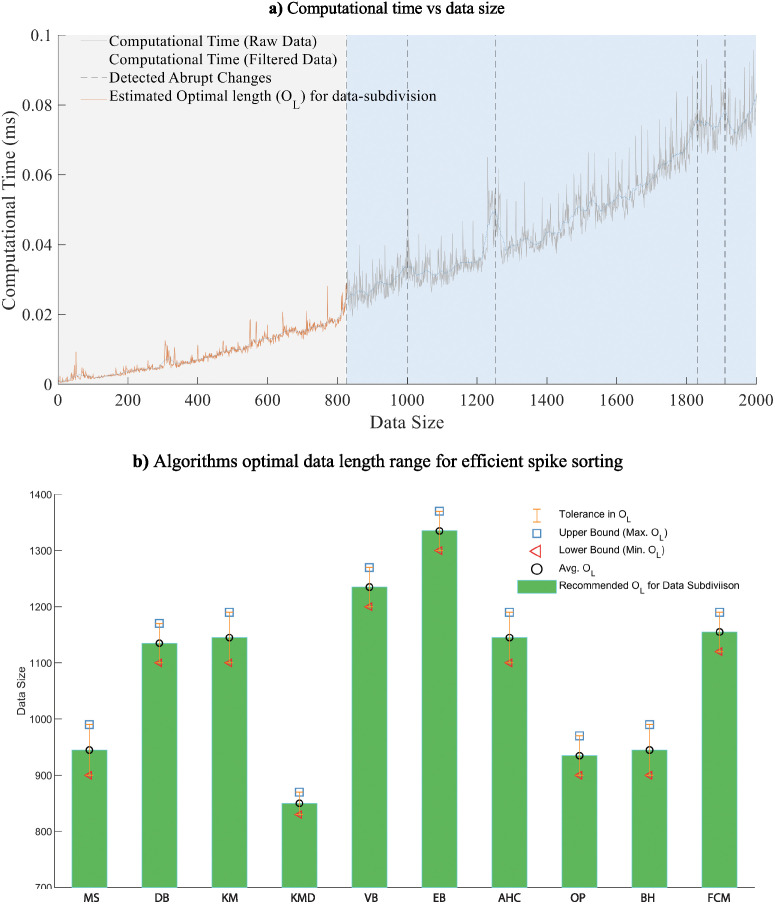
O_L is the range of values from which if the data size is selected to perform clustering, the clustering quality and computational efficiency of the conventional algorithms improve significantly. O_L parameter is dependent on the algorithm type rather than on the data dynamics. Therefore it needs to be estimated only once for each algorithm. The O_L parameter for ten commonly used clustering algorithms employed in this study, is estimated and shown in Fig 5b.

Fig 5. Identification of optimal length O_L.

(a) Illustrates the description of steps involved in identifying the O_L for spike sorting algorithms. Computational time versus data size plot. The X-axis shows the length of the data increasing from zero to 2000 while the Y-axis shows the corresponding time taken by the clustering algorithm to perform clustering process, in milliseconds. The computational time is the processing time after movmean filter(20 datapoints length) filtered the unwanted ripples in the plot and returned smooth curves. Detected abrupt changes in the plot taking 0.1 of the maximum rate of change in computational time as threshold (d) Identified optimal length O_L of data subsets used for data subdivision. b) Optimal Length (O_L) for ten commonly used clustering algorithms. The average value over ten repetitive analyses is given as robustness of the measure in optimal length for data subdivision.

To understand the computational time vs data size behaviour, clustering is performed in an incremental manner. At every increment, the size or length of the data increases and the computational time is plotted with respect to data size as shown in Fig 5a. The size of data for which the clustering algorithm shows smoother behaviour is termed as O_L, that needs to be estimated for optimal clustering results.

In this research work O_L is estimated by employing the work of Killick [66]. A threshold of 0.1 of the maximum rate of change of the computational time is used. The first change in computational time above the threshold is estimated to be the optimal length of the data-subset.

The procedure proposed in this research work to calculate O_L is implemented on ten aforementioned commonly used clustering algorithms. The procedure is repeated hundred times to get an average O_L value as an efficient measure for robustness in results. The calculated $O_L^{\prime }s$ are depicted in Fig 5b. It is observed that the performance of clustering algorithms is independent of the data dynamics and feature extraction techniques. O_L for all the algorithms adopted in this study, lies approximately in the same range for all three data and six feature sets, employed. Therefore, the computational performance of the algorithms depends on the length of the data set and not on the data dynamics.

Deviation of (O_L) from the estimated optimal point could lead to inefficient spike sorting performance. Data subdivision using optimal length is a compromise between computations involved in clustering process and unification process. (O_L) forms a direct relationship with clustering computations and an inverse relationship with computations involved in the unification process.

Clustering of data

Data subdivision is followed by clustering of data-subsets employing conventional spike sorting algorithms. Ten algorithms, as illustrated in Fig 5, are employed in this study due to their wide adaptability in spike sorting research. The algorithm proposed is independent of the clustering procedure; therefore, any other clustering technique could be adopted in this mechanism.

Unification of subclusters

After the clustering is performed on each data-subset, the unification of the sub clusters is performed. Sub-clusters are unified by identifying the overlap between the bounded regions of sub-clusters. The bounded region (BR) is a ‘m’ dimensional set which consist of minimum and maximum variations of ‘m’ dimensional spike feature waveforms in each dimension for a corresponding sub cluster. The bounded region for j^th sub cluster is given by relationship in Eq (3).

$$\begin{array}{c}\hfill B{R}_{j,i}=\left\{\begin{array}{c}{\left[\begin{array}{c}min\\ max\end{array}\right]}_{j,1}{\left[\begin{array}{c}min\\ max\end{array}\right]}_{j,2}{\left[\begin{array}{c}min\\ max\end{array}\right]}_{j,3}\cdots {\left[\begin{array}{c}min\\ max\end{array}\right]}_{j,m}\end{array}\right\}\end{array}$$ (3)

Where BR_j,i is the ‘m’ dimensional bounded region for j^th sub cluster with j ∈ [1, 2, 3,.., k] and ‘k’ is the total number of sub clusters participated in the unification process. ${\left[\begin{array}{c}min\\ max\end{array}\right]}_{j,i}$ are the minimum and maximum variations of spike feature waveforms for j^th sub cluster and in i^th dimension and i ∈ [1, 2, 3, …, m].

In this study, since 10 PCA or 10 Wavelet features are used to transform the spike waveform into spike feature waveform. So ‘m’ is 10 in this particular case and BR is a 10 dimensional set with minimum and maximum values providing variation of spike feature waveforms in each dimension for a particular sub cluster.

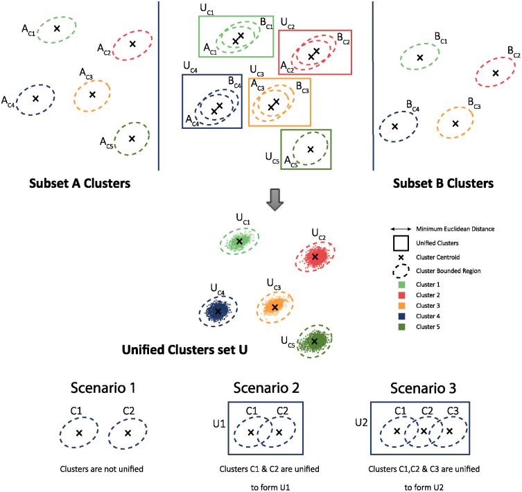
The bounded region is calculated for all ‘k’ sub clusters participated in the unification process. The sub clusters, having overlapping bounded regions in all dimensions, are unified together. The unification process for a 2 dimensional sub clusters is shown in Fig 6. In the Fig 6, it is also illustrated how sub clusters unify in three different scenarios i.e. 1) no overlapping region between sub clusters 2) overlap between two distinct sub clusters and 3) multiple overlapping sub clusters.

Fig 6. Mechanisim to unify or merge clusters.

To eliminate the impact of outliers in deciding the bounded region for unification process, the spike feature waveforms are filtered in each sub clusters. The filter proposed in this study is based on Euclidean distance. A sub cluster having ‘m’ dimensional spike feature waveforms, should have an ‘m’ dimensional centroid ‘C’. It is important to note that, the complete ‘m’ dimensional spike feature waveform is considered as a single point in ‘m’ dimensional space in calculating the Euclidean distance. Therefore, for each spike feature waveform, an Euclidean distance from spike feature waveform to its sub cluster centroid is calculated. The relationship to calculate the Euclidean distances is given in Eq (4).

$$\begin{array}{c}\hfill E{D}_l(C_i,S_{l,i})=\sqrt{{(C_1-S_{l,1})}^2+{(C_2-S_{l,2})}^2+{(C_3-S_{l,3})}^2+\cdots +{(C_m-S_{l,m})}^2}\end{array}$$ (4)

ED_l(C_i, S_l,i) is the Euclidean distance calculated for the l^th spike feature waveform S_l,i and sub cluster centroid C_i. l ∈ [1, 2, 3, 4 …, n] and i ∈ [1, 2, 3, …, m] where ‘n’ is the total number of spikes in a sub cluster and ‘m’ is the spike feature waveform dimension.

Since, the Euclidean distance is calculated based on Eq (4), a n × 1 Euclidean distance matrix (EDM) is generated, as in Eq (5).

$$\begin{array}{c}\hfill EDM=\left[\begin{array}{c}E{D}_1\\ E{D}_2\\ E{D}_3\\ ⋮\\ E{D}_n\end{array}\right]\end{array}$$ (5)

This EDM matrix is used to identify outliers in spike feature waveforms. From EDM, a Mean ‘μ’ and Standard Deviation ‘σ’ is calculated by using Eqs (6) and (7).

$$\begin{array}{c}\hfill \mu =\frac{{\sum }_{t=1}^{n}E{D}_t}{n}\end{array}$$ (6)

$$\begin{array}{c}\hfill \sigma =\sqrt{\frac{1}{n}\sum _{t=1}^n{(E{D}_t-\mu )}^2}\end{array}$$ (7)

Using the mean and standard deviation of a normal distribution curve, the Euclidean distance values are converted into Z scores using the Eq (8).

$$\begin{array}{c}\hfill Z_l=(E{D}_l-\mu )/\sigma \end{array}$$ (8)

The Z score distribution determined by Eq (8) is then used to identify the data outliers in the EDM matrix given by Eq (5). To this aim, we considered two scenarios; 1) when the Z score distribution of the EDM matrix is normal and 2) when the Z score distribution of the EDM matrix is skewed. There are numerous methods that can determine the normality of the data distribution as in [67–69]. However, in this study, the normality of the Z score distribution of EDM matrix is determined using the Interquartile Range IQR method [70].

The quartiles are three points that divide the data set into four equal groups, each group comprising a quarter of the data, for a set of data values which are arranged in either ascending or descending order. Q1, Q2, and Q3 are represent the first, second, and third quartile’s value. The Interquartile Range (IQR) is basically a difference between the first quartile (Q1) and third quartile (Q3). The IQR of the Euclidean distance matrix sorted in ascending order can be determined using relation given in Eq (9).

$$\begin{array}{c}\hfill IQR=Q3-Q1\end{array}$$ (9)

Where Q1 is first quartile and it is the median of lower half of the euclidean distances sorted in ascending order and Q3 is the third quartile and it is the median of upper half of the euclidean distances sorted in ascending order.

If the distance of the Q1 and Q3 from the median of the complete dataset containing Euclidean distances is equal, the data is normally distributed and the bell shaped curve is symmetric. If the distance from data mid-point to Q1 is bigger than Q3, the data distribution is skewed towards left, and if Q3 is bigger than Q1, the data distribution is skewed towards right.

For a normal distribution of the data, when bell shaped curve is symmetric, Empirical rule is valid and the outlier filter (OF) is is defined as a range between μ±2σ and its is given by Eq (10).

$$\begin{array}{c}\hfill OF=\left[\begin{array}{cc}min& max\end{array}\right]=\left[\begin{array}{cc}\mu -2\sigma & \mu +2\sigma \end{array}\right]=\left[\begin{array}{cc}-2Z& 2Z\end{array}\right]\end{array}$$ (10)

For a nonsymmetric or left and right skewed distributions, 1.5 Interquartile Range (1.5 IQR) filter is used to identify the sub cluster outliers. The factor 1.5 is empirically derived and being used by novel researchers in statistics for skewed data to identify outliers [71, 72]. Therefore, in this study 1.5 IQR based outlier filter (OF) is designed to remove data outliers in skewed distribution and it is given by Eq (11).

$$\begin{array}{c}\hfill OF=\left[\begin{array}{cc}min& max\end{array}\right]=\left[\begin{array}{cc}Q1-1.5\times IQR& Q3+1.5\times IQR\end{array}\right]\end{array}$$ (11)

All the featured spikes, having the Euclidean distance lies within the OF range, are considered in estimating the bounded region in Eq (3) for unification of sub clusters.

A similar approach is adopted by Aksenova et al. in [73] to perform training of online spike sorting algorithm employing phase space. Their algorithm is focused on efficient noise reduction rather than optimisation of computational efficiency.

Performance evaluation of the proposed algorithm

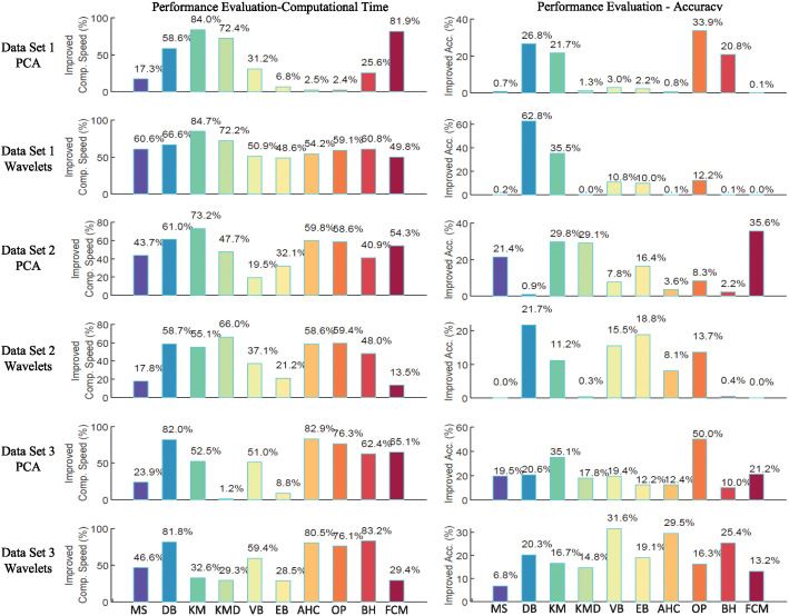
In this research work, the performance of the proposed algorithm is evaluated using two indicators, computational time and clustering quality. A comparative performance of the proposed algorithm with respect to the conventional algorithm is presented in Fig 7(a) and 7(b).

Fig 7. Illustration of improved computational speed and clustering accuracy.

(a) Improved computational speed in percentage of understudy ten algorithms across six large neural feature sets. (b) Improved clustering accuracy in percentage of understudy ten algorithms across six large neural feature sets. The proposed data-subdivision and unification method has shown a positive trend in improving the performance of spike sorting algorithms. The improvement in reducing computational time is significantly high, while due to maturity of spike of sorting algorithms, accuracy improvement is relatively lower in some of spike sorting algorithms. The average results for 10 repetitive analysis has been presented and it is worth noting that proposed mechanism has shown promising improvement results around all data types and spike sorting algorithms.

For validation, ten most widely adopted clustering algorithms are employed in the proposed research work. The algorithms include MeanShift (MS) [74], Density-based spatial clustering of applications with noise (DBSCAN) [75], Kmeans (KM) [76], Kmedoids (KMD) [77], Fuzzy C means (FCM) [78], Variational Bayesian Gaussian Mixture Model (VBGMM) [79], Expectation Maximization Gaussian Mixture Model (EMGMM) [80], Agglomerative Hierarchical Clustering (AHC) [81], Birch (BH) [82] and Ordering Points to Identify the Clustering Structure (OPTICS) [83].

To quantify computational efficiency of the proposed algorithm, three data sets are used, reported by Quiroga [84], because of their wider adoptability and ground truth availability. These datasets includes two (2) simulated Dataset 1 (D1) and Dataset 2 (D2) and one human Dataset 3 (D3). Human data is originated from multiunit recording in the temporal lobe of an epileptic patient from Itzhak Fried’s lab at UCLA [84]. The information regarding spatio-temporally overlapping spikes as a result of multi-unit recordings can be identified using “Matching Persuit” algorithm [85]. However in this study, the multi-unit spikes are already detected and labeled in the ground truth. Labels for three distinguished clusters are provided for each of dataset D1, D2 and D3 in their respective ground truth.

Each spike waveform consists of 64 samples. Haar Wavelets and PCA features are employed to reduce the data dimensionality while preserving the variance of the data and spike information. In case of Haar wavelets transform, optimal wavelet features were selected following the study of Quiroga [79], which implemented the four-level multi resolution decomposition. The 64 wavelet coefficients generated provides unique spike characteristic at different scales and times. As each spike class has different multimodal distribution, the Lilliefors modification of Kolmogorov-Smirnov (KS) test for normality [81] was used to select the optimal wavelet features. The maximum deviation of multimodal distribution features from normality defines the optimal features. We refer the readers to Quiroga [79] for further explanation. In this context, 10 wavelet features with largest deviation of normality is regarded as optimal wavelet features.

Similarly, 10 PCA features were selected in this study to validate the computational and performance efficiency of the proposed vs conventional algorithms. The PCA components are not scaled to match their explained variances. The individual variances of PCA components are accumulated and the optimal number of PCA components that gives at least 85% of cumulative explained variance are chosen for the analysis. 10 PCA features are required to get at least 85% cumulative explained variance of the 64 dimensional spikes data used in this study.

It is important to note that, the accuracy of clustering algorithms may be affected by the data dimensionality and number of optimal feature sets used. However, in this study the same 10-dimensional features are used for all the algorithms to maintain the consistency while validating the performance outcomes.

The research work is carried out on a personal computer (PC) consisting of Intel (R) Pentium (R) CPU G4560 @3.5GHz, 8 GB of RAM and 64 Bit windows 10 operating system.

Performance on computational time or speed

To explore and validate the performance of the proposed algorithm, in terms of computational time, as tabulated in Table 2, is estimated using the expression (12).

$$\begin{array}{c}\hfill T_s(\%)=\frac{(C_t-P_t)}{C_t}\times 100\end{array}$$ (12)

Table 2. Computational times and time based performance improvement for ten clustering algorithms.

Algorithm	Method	Computational Time (Seconds)
		D1, PCA	D1, WAV	D2, PCA	D2, WAV	D3, PCA	D3, WAV
Meanshift	Proposed	0.3	0.02	0.43	0.13	0.11	0.03
	Conventional	0.36	0.04	0.76	0.16	0.15	0.06
	Time Saved (%)	17.25	60.59	43.69	17.81	23.88	46.63
DBSCAN	Proposed	0.75	1.6	3.26	0.54	8.76	3.84
	Conventional	1.82	4.81	8.37	1.3	48.63	21.09
	Time Saved (%)	58.6	66.64	61.02	58.71	81.98	81.77
Kmeans	Proposed	0.04	0	0.01	0	0.04	0.03
	Conventional	0.28	0.03	0.03	0.01	0.09	0.05
	Time Saved (%)	84	84.7	73.2	55.14	52.55	32.59
Kmedoids	Proposed	0.32	0.1	0.17	0.14	1.37	1.31
	Conventional	1.14	0.36	0.33	0.41	1.38	1.85
	Time Saved (%)	72.39	72.2	47.67	65.99	1.19	29.26
VBGMM	Proposed	0.3	0.25	0.6	0.4	1.91	1.05
	Conventional	0.44	0.51	0.75	0.63	3.9	2.57
	Time Saved (%)	31.17	50.85	19.46	37.15	51.02	59.35
EMGMM	Proposed	0.43	0.32	1.2	0.46	3.39	3.07
	Conventional	0.46	0.62	1.76	0.58	3.71	4.29
	Time Saved (%)	6.83	48.56	32.06	21.17	8.78	28.5
Agglomerative	Proposed	0.18	0.07	0.06	0.06	0.2	0.2
	Conventional	0.18	0.15	0.15	0.14	1.14	1.04
	Time Saved (%)	2.55	54.23	59.75	58.61	82.92	80.46
OPTICS	Proposed	1.11	0.44	0.42	0.43	1.72	1.72
	Conventional	1.14	1.08	1.02	1.05	7.27	7.18
	Time Saved (%)	2.35	59.15	58.56	59.37	76.34	76.07
BIRCH	Proposed	1.25	1.61	1.39	1.94	2.22	5.32
	Conventional	1.68	4.11	2.35	3.73	5.9	31.56
	Time Saved (%)	25.65	60.77	40.94	47.99	62.4	83.15
FCM	Proposed	0.01	0.03	0.01	0.05	0.02	0.41
	Conventional	0.08	0.05	0.02	0.06	0.05	0.59
	Time Saved (%)	81.92	49.8	54.26	13.51	65.12	29.43

Where C_t and P_t are computational times of clustering using conventional and proposed algorithms, respectively.

Performance on clustering accuracy

The clustered spikes from spike sorting algorithms are generally evaluated using the validation indices [46]. In this work clustering accuracy, as is described in [86] and (13), is adopted as a validation index and is calculated using the confusion matrix [87] as in (14).

$$\begin{array}{c}\hfill A=\frac{\#ofaccuratelyclusteredspikes}{Total\#ofSpikes}\%=\frac{SumofConf.MatrixDiagonals}{Total\#ofSpikes}\%\end{array}$$ (13)

$$\begin{array}{c}\hfill C=\left[\begin{array}{ccc}{C}_{e_1{g}_1}& C_{e_1{g}_2}\dots & C_{e_1{g}_q}\\ C_{e_2{g}_1}& C_{e_2{g}_2}\dots & C_{e_2{g}_q}\\ \begin{array}{c}.\\ .\\ .\end{array}& \begin{array}{c}.\\ .\\ .\end{array}& \begin{array}{c}.\\ .\\ .\end{array}\\ C_{e_m{g}_1}& C_{e_m{g}_2}\dots & C_{e_m{g}_q}\end{array}\right]\end{array}$$ (14)

Where A and C are accuracy index and confusion matrix, respectively. m is total number of estimated clusters and q is total number of clusters in ground truth. $C_{e_i,g_i}$ represents the number of spikes estimated and clustered accurately relative to the labels provided with the spikes data ground truth. Where e_i refers to estimated cluster index and g_i ground truth. The accuracy index highlights the percentage of spikes accurately labelled to the clusters described in the ground truth. There are two scenarios taken into account while calculating accuracies.

m = q: when number of clusters estimated are equal to number of clusters in the ground truth. This leads to the square confusion matrix of size m|_m=q and the sum of confusion matrix diagonals divided by total number of spikes provides the percentage of accuracy as in Eq (13).

m ≠ q: when the number of clusters estimated m are not equal to the number of clusters in ground truth q, the confusion matrix is generated by taking only the dominant estimated clusters m equal to the total number of clusters q in the ground truth. In case of estimated clusters less than the ground truth clusters, i.e. m < q, the confusion matrix is zero padded. The accuracy is calculated by using the expression (13).

The percentage of accuracy enhancement is estimated using the accuracy difference between proposed and conventional methods, which is tabulated in Table 3.

Table 3. Clustering accuracy and accuracy based performance improvement for ten clustering algorithms.

Algorithm	Method	Accuracy (%)
		D1, PCA	D1, WAV	D2, PCA	D2, WAV	D3, PCA	D3, WAV
Meanshift	Proposed	89.89	97.81	83.76	94.03	72.18	81.82
	Conventional	89.18	97.59	62.36	94	52.72	75.05
	Improved Acc. (%)	0.71	0.23	21.4	0.03	19.46	6.76
DBSCAN	Proposed	87.85	92.16	34.72	84.02	72.18	72.19
	Conventional	61.07	35.29	33.79	62.3	51.55	51.88
	Improved Acc. (%)	26.77	56.87	0.93	21.72	20.63	20.32
Kmeans	Proposed	66.35	99.38	95.21	92.78	71.63	78.87
	Conventional	44.69	63.86	65.46	81.58	36.56	62.21
	Improved Acc. (%)	21.66	35.52	29.76	11.19	35.06	16.66
Kmedoids	Proposed	98.07	99.38	77.52	93.1	61.31	83.92
	Conventional	96.79	99.38	48.46	92.78	43.48	69.14
	Improved Acc. (%)	1.28	0	29.06	0.32	17.82	14.78
VBGMM	Proposed	88.25	77.31	62.3	84.34	70.08	63.51
	Conventional	85.26	66.47	54.52	68.85	50.66	31.93
	Improved Acc. (%)	2.98	10.85	7.77	15.49	19.42	31.58
EMGMM	Proposed	91.31	90.37	72.97	84.66	74.15	57.21
	Conventional	89.15	80.41	56.61	65.84	61.95	38.15
	Improved Acc. (%)	2.16	9.97	16.36	18.82	12.2	19.05
Agglomerative	Proposed	94.55	99.26	88.46	96	56.15	80.88
	Conventional	93.7	99.21	84.86	87.91	43.75	51.4
	Improved Acc. (%)	0.85	0.06	3.6	8.09	12.4	29.48
OPTICS	Proposed	76.58	29.42	31	26.04	62.33	20.58
	Conventional	42.67	17.18	22.71	12.38	12.34	4.28
	Improved Acc. (%)	33.9	12.24	8.29	13.66	49.99	16.29
BIRCH	Proposed	93.19	99.26	86.83	93.33	54.73	80.88
	Conventional	72.43	99.18	84.66	92.89	44.76	55.53
	Improved Acc. (%)	20.76	0.09	2.18	0.44	9.96	25.35
FCM	Proposed	71.78	99.38	84.98	92.63	60.99	77.15
	Conventional	71.72	99.38	49.42	92.6	39.77	63.97
	Improved Acc. (%)	0.06	0	35.56	0.03	21.22	13.18

Clustering results

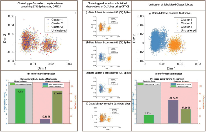
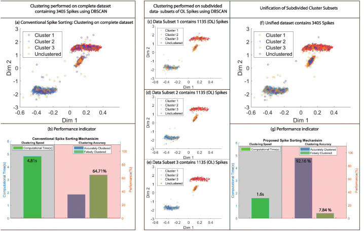
To highlight enhancement in clustering quality, visual representation of clusters estimated using proposed and conventional methods employing OPTICS on dataset 3 with PCA features and DBSCAN on dataset 1 with Wavelet features, gives 49.99 and 56.87 percent accuracy improvement in the clustering results with respect to the ground truth as in Table 3. The illustration of clustering results for aforementioned examples is shown in Figs 8 and 9 respectively. It is clear from the results that proposed methodology generates significantly superior results in contrast to conventional methods.

Fig 8. Comparison of clustering results obtained using conventional and proposed mechanism employing OPTICS with dataset 3 and PCA features.

(a) Clustering results using conventional spike sorting method applied on complete dataset containing 3740 Spikes. (b) Performance indication of clustering results based on computational time/speed and clustering accuracy. (c)-(f) Clustering results using proposed spike sorting mechanism applied on data-subdivision of optimal length i.e 935 for OPTICS. (g) Unification of subdivided cluster subsets. (h) Performance indication of clustering results using proposed spike sorting method.

Fig 9. Comparison of clustering results obtained using conventional and proposed mechanism employing DBSCAN with dataset 1 and Wavelet features.

(a) Clustering results using conventional spike sorting method applied on complete dataset containing 3405 Spikes. (b) Performance indication of clustering results based on computational time/speed and clustering accuracy. (c)-(f) Clustering results using proposed spike sorting mechanism applied on data-subdivision of optimal length i.e 1135 for DBSCAN. (g) Unification of subdivided cluster subsets. (h) Performance indication of clustering results using proposed spike sorting method.

Discussion

It is largely observed from the results and performance evaluation that the proposed algorithm shows continuous improvement around all algorithms and datasets. The accuracy is improved up to 56.87% while computational time is reduced up to 84.7%. Hence, proposed mechanism has significant impact on enhancing the speed and accuracy of the spike sorting process. In term of clustering accuracy, DBSCAN demonstrates high accuracy improvement of 56.87 percent followed by OPTICS at 49.99 percent. In terms of computational time, Kmeans shows highest computational speed enhancement of 84.7 percent followed by BIRCH with computational speed enhancement of 83.15 percent. In terms of parameter tuning complexity, MeanShift, FCM and Gaussian Mixture models require one parameter to tune, DBSCAN and OPTICS require two and BIRCH requires three parameters to tune to perform their operations. All the supervised clustering algorithms including Kmeans, Kmedoids and Agglomerative require single parameter to tune. In terms of robustness, Kmeans, Kmedoids,FCM gives different results at every iteration, however, Meanshift, EMGMM, VMGMM, Agglomerative, DBSCAN, OPTICS, BIRCH converged to same results after each iteration. For simplicity of the presentation, the presented results are averaged over 10 repetitions.

Software implementation

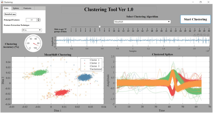
The software for proposed mechanism is implemented using MATLAB as shown in Fig 10. The free access to open source software for academic purpose is provided with detailed user instructions online at: https://github.com/ermasood/Handling-Larger-Data-Sets-for-Clustering. The software yields the clustering labels with high accuracy and in a fast and efficient way. The first graph in the software window shows the clustered spikes and the second graph illustrates the clustered features of the inputted data. MATLAB codes provided are tested on 2019b and 2018b MATLAB versions. Additionally,’Linspecer.m’ file [88] from MathWorks is required to generate attractive colour combinations and shades for beautiful visualisations.

Fig 10. Software for proposed clustering mechanism.

Conclusion

Neural spike sorting is prerequisite to deciphering useful information from electrophysiological data recorded from the brain, in vitro and/or in vivo. Significant advancements in nanotechnology and nano fabrication has enabled neuroscientists and engineers to capture the electrophysiological activities of the brain at very high resolution, data rate and fidelity. However, the evolution in spike sorting algorithms to deal with the aforementioned technological advancement and capability to quantify higher density data sets is somewhat limited. It is observed from the experiments that larger datasets highly effect the computational time required to perform clustering. To address this challenge, a novel clustering mechanism is proposed to handle large datasets efficiently and with higher accuracy. The proposed mechanism resolves the issue of high computational time and reduced accuracy in conventional method. The proposed algorithms has demonstrated up to 84% and 56% improvement in terms of computational time and clustering accuracy, respectively. The proposed framework is validated by applying on ten widely used clustering algorithms and six large data sets. PCA and Haar wavelets features are employed for consistency during the clustering process. A MATLAB software of the proposed mechanism is also developed and provided to assist the researchers, active in this domain.

Supporting information

S1 Data

(ZIP)

Data Availability

All relevant data are within the manuscript and its Supporting information files.

Funding Statement

The research work is fully supported by Neural and Cognitive Systems Lab at Institute for Intelligent Systems Research and Innovation, Deakin University". Although we do not have any explicit external funding grant linked to this work however the work is internally funded by the lab.

References

- 1. Dominique MD. What is Neural Engineering? Journal of Neural Engineering. 2006;4(4). [Google Scholar]
- 2. Bhatti A, Lee KH, Garmestani H, Lim CP. Emerging Trends in Neuro Engineering and Neural Computation. Springer; 2017. [Google Scholar]
- 3. He B. Neural engineering. Springer Science & Business Media; 2007. [Google Scholar]
- 4. Eliasmith C, Anderson CH. Neural engineering. Massachusetts Institue of Technology; 2003;. [Google Scholar]
- 5. Gaburro J, Bhatti A, Harper J, Jeanne I, Dearnley M, Green D, et al. Neurotropism and behavioral changes associated with Zika infection in the vector Aedes aegypti. 2018;7(1):1–11. [DOI] [PMC free article] [PubMed] [Google Scholar]
- 6. Gaburro J, Duchemin JB, Paradkar PN, Nahavandi S, Bhatti AJSr. Electrophysiological evidence of RML12 mosquito cell line towards neuronal differentiation by 20-hydroxyecdysdone. 2018;8(1):10109. [DOI] [PMC free article] [PubMed] [Google Scholar]
- 7. Bari MAU, Gaburro J, Michalczyk A, Ackland ML, Williams C, Bhatti A. In: Mechanism of Docosahexaenoic Acid in the Enhancement of Neuronal Signalling. Springer; 2017. p. 99–117. [Google Scholar]
- 8. Gaburro J, Bhatti A, Sundaramoorthy V, Dearnley M, Green D, Nahavandi S, et al. Zika virus-induced hyper excitation precedes death of mouse primary neuron. 2018;15(1):79. [DOI] [PMC free article] [PubMed] [Google Scholar]
- 9. Mussa-Ivaldi FA, Miller LE. Brain–machine interfaces: computational demands and clinical needs meet basic neuroscience. TRENDS in Neurosciences. 2003;26(6):329–334. 10.1016/S0166-2236(03)00121-8 [DOI] [PubMed] [Google Scholar]
- 10. Lefebvre JL, Zhang Y, Meister M, Wang X, Sanes JR. Y-Protocadherins regulate neuronal survival but are dispensable for circuit formation in retina. Development. 2008;135(24):4141–4151. 10.1242/dev.027912 [DOI] [PMC free article] [PubMed] [Google Scholar]
- 11. Lee AK, Manns ID, Sakmann B, Brecht M. Whole-Cell Recordings in Freely Moving Rats. Neuron. 2006;51(4):399–407. 10.1016/j.neuron.2006.07.004 [DOI] [PubMed] [Google Scholar]
- 12. Spira ME, Hai A. Multi-electrode array technologies for neuroscience and cardiology. Nature nanotechnology. 2013;8(2):83 10.1038/nnano.2012.265 [DOI] [PubMed] [Google Scholar]
- 13. Stuart G, Dodt H, Sakmann B. Patch-clamp recordings from the soma and dendrites of neurons in brain slices using infrared video microscopy. Pflügers Archiv. 1993;423(5-6):511–518. [DOI] [PubMed] [Google Scholar]
- 14. Zhang J, Laiwalla F, Kim JA, Urabe H, Van Wagenen R, Song YK, et al. Integrated device for optical stimulation and spatiotemporal electrical recording of neural activity in light-sensitized brain tissue. Journal of neural engineering. 2009;6(5):055007 10.1088/1741-2560/6/5/055007 [DOI] [PMC free article] [PubMed] [Google Scholar]
- 15. Cui X, Lee VA, Raphael Y, Wiler JA, Hetke JF, Anderson DJ, et al. Surface modification of neural recording electrodes with conducting polymer/biomolecule blends. Journal of Biomedical Materials Research. 2001;56(2):261–272. [DOI] [PubMed] [Google Scholar]
- 16. Buzsáki G. Large-scale recording of neuronal ensembles. Nature neuroscience. 2004;7(5):446 10.1038/nn1233 [DOI] [PubMed] [Google Scholar]
- 17. Wise KD, Najafi K. Microfabrication techniques for integrated sensors and microsystems. Science. 1991;254(5036):1335–1342. 10.1126/science.1962192 [DOI] [PubMed] [Google Scholar]
- 18. Csicsvari J, Henze DA, Jamieson B, Harris KD, Sirota A, Barthó P, et al. Massively parallel recording of unit and local field potentials with silicon-based electrodes. Journal of neurophysiology. 2003;90(2):1314–1323. 10.1152/jn.00116.2003 [DOI] [PubMed] [Google Scholar]
- 19. Zhang J, Nguyen T, Cogill S, Bhatti A, Luo L, Yang S, et al. A review on cluster estimation methods and their application to neural spike data. Journal of neural engineering. 2018;15(3). 10.1088/1741-2552/aab385 [DOI] [PubMed] [Google Scholar]
- 20. Veerabhadrappa R, Lim C, Nguyen T, Berk M, Tye S, Monaghan P, et al. Unified selective sorting approach to analyse multi-electrode extracellular data. Scientific reports. 2016;6:28533 10.1038/srep28533 [DOI] [PMC free article] [PubMed] [Google Scholar]
- 21. Khudhair D, Nahavandi S, Garmestani H, Bhatti A. In: Microelectrode Arrays: Architecture, Challenges and Engineering Solutions. Springer; 2017. p. 41–59. [Google Scholar]
- 22. Veerabhadrappa R, Bhatti A, Berk M, Tye SJ, Nahavandi S. Hierarchical estimation of neural activity through explicit identification of temporally synchronous spikes. Neurocomputing. 2017;249:299–313. 10.1016/j.neucom.2016.09.135 [DOI] [Google Scholar]
- 23. Hettiarachchi IT, Lakshmanan S, Bhatti A, Lim C, Prakash M, Balasubramaniam P, et al. Chaotic synchronization of time-delay coupled Hindmarsh–Rose neurons via nonlinear control. Nonlinear dynamics. 2016;86(2):1249–1262. 10.1007/s11071-016-2961-4 [DOI] [Google Scholar]
- 24. Rey HG, Pedreira C, Quiroga RQ. Past, present and future of spike sorting techniques. Brain research bulletin. 2015;119:106–117. 10.1016/j.brainresbull.2015.04.007 [DOI] [PMC free article] [PubMed] [Google Scholar]
- 25. Kreuz T, Chicharro D, Houghton C, Andrzejak RG, Mormann F. Monitoring spike train synchrony. Journal of neurophysiology. 2012;109(5):1457–1472. 10.1152/jn.00873.2012 [DOI] [PubMed] [Google Scholar]
- 26. Brown EN, Kass RE, Mitra PP. Multiple neural spike train data analysis: state-of-the-art and future challenges. Nature neuroscience. 2004;7(5):456 10.1038/nn1228 [DOI] [PubMed] [Google Scholar]
- 27. Einevoll GT, Franke F, Hagen E, Pouzat C, Harris KD. Towards reliable spike-train recordings from thousands of neurons with multielectrodes. Current opinion in neurobiology. 2012;22(1):11–17. 10.1016/j.conb.2011.10.001 [DOI] [PMC free article] [PubMed] [Google Scholar]
- 28.Zhou H, Mohamed S, Bhatti A, Lim CP, Gu N, Haggag S, et al. Spike sorting using hidden markov models. In: International Conference on Neural Information Processing. Springer;. p. 553–560.
- 29. Choi JH, Jung HK, Kim T. A new action potential detector using the MTEO and its effects on spike sorting systems at low signal-to-noise ratios. IEEE Transactions on Biomedical Engineering. 2006;53(4):738–746. 10.1109/TBME.2006.870239 [DOI] [PubMed] [Google Scholar]
- 30. Paralikar KJ, Rao CR, Clement RS. New approaches to eliminating common-noise artifacts in recordings from intracortical microelectrode arrays: Inter-electrode correlation and virtual referencing. Journal of neuroscience methods. 2009;181(1):27–35. 10.1016/j.jneumeth.2009.04.014 [DOI] [PMC free article] [PubMed] [Google Scholar]
- 31. Takekawa T, Ota K, Murayama M, Fukai T. Spike detection from noisy neural data in linear-probe recordings. European Journal of Neuroscience. 2014;39(11):1943–1950. 10.1111/ejn.12614 [DOI] [PubMed] [Google Scholar]
- 32. Gibson S, Judy JW, Marković D. Spike sorting: The first step in decoding the brain: The first step in decoding the brain. IEEE Signal processing magazine. 2012;29(1):124–143. 10.1109/MSP.2011.941880 [DOI] [Google Scholar]
- 33. Abeles M, Goldstein MH. Multispike train analysis. Proceedings of the IEEE. 1977;65(5):762–773. 10.1109/PROC.1977.10559 [DOI] [Google Scholar]
- 34. Abe S. In: Feature selection and extraction. Springer; 2010. p. 331–341. [Google Scholar]
- 35. Adamos DA, Kosmidis EK, Theophilidis G. Performance evaluation of PCA-based spike sorting algorithms. Computer methods and programs in biomedicine. 2008;91(3):232–244. 10.1016/j.cmpb.2008.04.011 [DOI] [PubMed] [Google Scholar]
- 36. Zamani M, Demosthenous A. Feature extraction using extrema sampling of discrete derivatives for spike sorting in implantable upper-limb neural prostheses. IEEE Transactions on Neural Systems and Rehabilitation Engineering. 2014;22(4):716–726. 10.1109/TNSRE.2014.2309678 [DOI] [PubMed] [Google Scholar]
- 37. Shoham S, Fellows MR, Normann RA. Robust, automatic spike sorting using mixtures of multivariate t-distributions. Journal of neuroscience methods. 2003;127(2):111–122. 10.1016/S0165-0270(03)00120-1 [DOI] [PubMed] [Google Scholar]
- 38. Lagerlund TD, Sharbrough FW, Busacker NE. Spatial filtering of multichannel electroencephalographic recordings through principal component analysis by singular value decomposition. Journal of clinical neurophysiology. 1997;14(1):73–82. 10.1097/00004691-199701000-00007 [DOI] [PubMed] [Google Scholar]
- 39. Takekawa T, Isomura Y, Fukai T. Accurate spike sorting for multi-unit recordings. European Journal of Neuroscience. 2010;31(2):263–272. 10.1111/j.1460-9568.2009.07068.x [DOI] [PubMed] [Google Scholar]
- 40. Özkaramanli H, Bhatti A, Bilgehan B. Multi-wavelets from B-spline super-functions with approximation order. Signal processing. 2002;82(8):1029–1046. 10.1016/S0165-1684(02)00212-8 [DOI] [Google Scholar]
- 41.Bhatti A, Ozkaramanli H. M-band multi-wavelets from spline super functions with approximation order. In: Acoustics, Speech, and Signal Processing (ICASSP), 2002 IEEE International Conference on. vol. 4. IEEE;. p. IV–4172–IV–4172.
- 42. Hulata E, Segev R, Ben-Jacob E. A method for spike sorting and detection based on wavelet packets and Shannon’s mutual information. Journal of neuroscience methods. 2002;117(1):1–12. 10.1016/S0165-0270(02)00032-8 [DOI] [PubMed] [Google Scholar]
- 43. Hulata E, Segev R, Shapira Y, Benveniste M, Ben-Jacob E. Detection and sorting of neural spikes using wavelet packets. Physical review letters. 2000;85(21):4637 10.1103/PhysRevLett.85.4637 [DOI] [PubMed] [Google Scholar]
- 44.Hartigan JA. Clustering algorithms. 1975;.
- 45.Steinbach M, Karypis G, Kumar V. A comparison of document clustering techniques. In: KDD workshop on text mining. vol. 400. Boston;. p. 525–526.
- 46. Lewicki MS. A review of methods for spike sorting: the detection and classification of neural action potentials. Network: Computation in Neural Systems. 1998;9(4):R53–R78. 10.1088/0954-898X_9_4_001 [DOI] [PubMed] [Google Scholar]
- 47.Wehr M, Pezarisl J, Sahani M. Spike Sorting Algorithms;.
- 48.Eick CF, Zeidat N, Zhao Z. Supervised clustering-algorithms and benefits. In: Tools with Artificial Intelligence, 2004. ICTAI 2004. 16th IEEE International Conference on. IEEE;. p. 774–776.
- 49.Jain AK, Dubes RC. Algorithms for clustering data. 1988;.
- 50.Zhao Z. Evolutionary Computing and Splitting Algorithms for Supervised Clustering [Thesis]; 2004.
- 51.Gibson S, Judy JW, Markovic D. Comparison of spike-sorting algorithms for future hardware implementation. In: Engineering in Medicine and Biology Society, 2008. EMBS 2008. 30th Annual International Conference of the IEEE. IEEE;. p. 5015–5020. [DOI] [PubMed]
- 52. Stevenson IH, Kording KPJNn. How advances in neural recording affect data analysis. 2011;14(2):139. [DOI] [PMC free article] [PubMed] [Google Scholar]
- 53.Hassan MU, Veerabhadrappa R, Zhang J, Bhatti A. Robust Optimal Parameter Estimation (OPE) for Unsupervised Clustering of Spikes Using Neural Networks. In: 2020 IEEE International Conference on Systems, Man, and Cybernetics (SMC). IEEE; 2020. p. 1286–1291.
- 54. Veerabhadrappa R, Ul Hassan M, Zhang J, Bhatti A. Compatibility evaluation of clustering algorithms for contemporary extracellular neural spike sorting. Frontiers in systems neuroscience. 2020;14:34 10.3389/fnsys.2020.00034 [DOI] [PMC free article] [PubMed] [Google Scholar]
- 55. Wouters J, Kloosterman F, Bertrand A. Towards online spike sorting for high-density neural probes using discriminative template matching with suppression of interfering spikes. Journal of neural engineering. 2018;15(5):056005 10.1088/1741-2552/aace8a [DOI] [PubMed] [Google Scholar]
- 56.Rakesh Veerabhadrappa JZAB Masood Ul Hassan. Compliance Assessment of Clustering Algorithms for Future Contemporary Extracellular Neural Spike Sorting. Frontiers in Systems Neuroscience. 2020;. [DOI] [PMC free article] [PubMed]
- 57. Wild J, Prekopcsak Z, Sieger T, Novak D, Jech RJJonm. Performance comparison of extracellular spike sorting algorithms for single-channel recordings. 2012;203(2):369–376. [DOI] [PubMed] [Google Scholar]
- 58. Chung JE, Magland JF, Barnett AH, Tolosa VM, Tooker AC, Lee KY, et al. A fully automated approach to spike sorting. Neuron. 2017;95(6):1381–1394. 10.1016/j.neuron.2017.08.030 [DOI] [PMC free article] [PubMed] [Google Scholar]
- 59.Chen X, Cai D. Large scale spectral clustering with landmark-based representation. In: Twenty-Fifth AAAI Conference on Artificial Intelligence;.
- 60.LeCun Y. The MNIST database of handwritten digits. http://yann.lecun.com/exdb/mnist/;.
- 61. Bache K, Lichman M. UCI Machine Learning Repository [http://archive.ics.uci.edu/ml]. Irvine, CA: University of California; School of information and computer science. 2013;28. [Google Scholar]
- 62. Duarte MF, Hu YH. Vehicle classification in distributed sensor networks. Journal of Parallel and Distributed Computing. 2004;64(7):826–838. 10.1016/j.jpdc.2004.03.020 [DOI] [Google Scholar]
- 63. Napoleon D, Pavalakodi SJIJoCA. A new method for dimensionality reduction using k-means clustering algorithm for high dimensional data set. 2011;13(7):41–46. [Google Scholar]
- 64. Killick R, Fearnhead P, Eckley IAJJotASA. Optimal detection of changepoints with a linear computational cost. 2012;107(500):1590–1598. [Google Scholar]
- 65. Pachitariu M, Steinmetz N, Kadir S, Carandini M, Harris KD. Kilosort: realtime spike-sorting for extracellular electrophysiology with hundreds of channels. BioRxiv. 2016; p. 061481. [Google Scholar]
- 66. Dokmanic I, Parhizkar R, Ranieri J, Vetterli MJISPM. Euclidean distance matrices: essential theory, algorithms, and applications. 2015;32(6):12–30. [Google Scholar]
- 67. Drezner Z, Turel O, Zerom D. A modified Kolmogorov–Smirnov test for normality. Communications in Statistics—Simulation and Computation®. 2010;39(4):693–704. 10.1080/03610911003615816 [DOI] [Google Scholar]
- 68. Mbah AK, Paothong A. Shapiro–Francia test compared to other normality test using expected p-value. Journal of Statistical Computation and Simulation. 2015;85(15):3002–3016. 10.1080/00949655.2014.947986 [DOI] [Google Scholar]
- 69. Yazici B, Yolacan S. A comparison of various tests of normality. Journal of Statistical Computation and Simulation. 2007;77(2):175–183. 10.1080/10629360600678310 [DOI] [Google Scholar]
- 70. Mishra P, Pandey CM, Singh U, Gupta A, Sahu C, Keshri A. Descriptive statistics and normality tests for statistical data. Annals of cardiac anaesthesia. 2019;22(1):67 10.4103/aca.ACA_157_18 [DOI] [PMC free article] [PubMed] [Google Scholar]
- 71. Hubert M, Van der Veeken S. Outlier detection for skewed data. Journal of Chemometrics: A Journal of the Chemometrics Society. 2008;22(3-4):235–246. 10.1002/cem.1123 [DOI] [Google Scholar]
- 72. Rousseeuw PJ, Hubert M. Robust statistics for outlier detection. Wiley Interdisciplinary Reviews: Data Mining and Knowledge Discovery. 2011;1(1):73–79. [Google Scholar]
- 73. Aksenova TI, Chibirova OK, Dryga OA, Tetko IV, Benabid AL, Villa AE. An unsupervised automatic method for sorting neuronal spike waveforms in awake and freely moving animals. Methods. 2003;30(2):178–187. 10.1016/S1046-2023(03)00079-3 [DOI] [PubMed] [Google Scholar]
- 74.Ester M, Kriegel HP, Sander J, Xu X. A density-based algorithm for discovering clusters in large spatial databases with noise. In: Kdd. vol. 96;. p. 226–231.
- 75. Lloyd S. Least squares quantization in PCM. IEEE transactions on information theory. 1982;28(2):129–137. 10.1109/TIT.1982.1056489 [DOI] [Google Scholar]
- 76. Park HS, Jun CH. A simple and fast algorithm for K-medoids clustering. Expert systems with applications. 2009;36(2):3336–3341. 10.1016/j.eswa.2008.01.039 [DOI] [Google Scholar]
- 77. Bezdek JC, Ehrlich R, Full W. FCM: The fuzzy c-means clustering algorithm. Computers & Geosciences. 1984;10(2-3):191–203. 10.1016/0098-3004(84)90020-7 [DOI] [Google Scholar]
- 78. Corduneanu A, Bishop CM. Variational Bayesian model selection for mixture distributions In: Artificial intelligence and Statistics. vol. 2001 Morgan Kaufmann; Waltham, MA;. p. 27–34. [Google Scholar]
- 79. Law MH, Figueiredo MA, Jain AK. Simultaneous feature selection and clustering using mixture models. IEEE transactions on pattern analysis and machine intelligence. 2004;26(9):1154–1166. 10.1109/TPAMI.2004.71 [DOI] [PubMed] [Google Scholar]
- 80.Davidson I, Ravi S. Agglomerative hierarchical clustering with constraints: Theoretical and empirical results. In: European Conference on Principles of Data Mining and Knowledge Discovery. Springer;. p. 59–70.
- 81.Zhang T, Ramakrishnan R, Livny M. BIRCH: an efficient data clustering method for very large databases. In: ACM Sigmod Record. vol. 25. ACM;. p. 103–114.
- 82.Ankerst M, Breunig MM, Kriegel HP, Sander J. OPTICS: ordering points to identify the clustering structure. In: ACM Sigmod record. vol. 28. ACM;. p. 49–60.
- 83. Quiroga RQ. Concept cells: the building blocks of declarative memory functions. Nature Reviews Neuroscience. 2012;13(8):587 10.1038/nrn3251 [DOI] [PubMed] [Google Scholar]
- 84. Story M, Congalton RG. Accuracy assessment: a user’s perspective. Photogrammetric Engineering and remote sensing. 1986;52(3):397–399. [Google Scholar]
- 85.Do TT, Gan L, Nguyen N, Tran TD. Sparsity adaptive matching pursuit algorithm for practical compressed sensing. In: 2008 42nd Asilomar Conference on Signals, Systems and Computers. IEEE; 2008. p. 581–587.
- 86. Ben-David A. A lot of randomness is hiding in accuracy. Engineering Applications of Artificial Intelligence. 2007;20(7):875–885. 10.1016/j.engappai.2007.01.001 [DOI] [Google Scholar]
- 87. Dunham MH. Data mining: Introductory and advanced topics. Pearson Education; India; 2006. [Google Scholar]
- 88.Lansey JC. Beautiful and distinguishable line colors colormap—File Exchange - MATLAB Central;. Available from: https://au.mathworks.com/matlabcentral/fileexchange/42673-beautiful-and-distinguishable-line-colors-colormap.