Relaxed Random Walks at Scale

Abstract

Relaxed random walk (RRW) models of trait evolution introduce branch-specific rate multipliers to modulate the variance of a standard Brownian diffusion process along a phylogeny and more accurately model overdispersed biological data. Increased taxonomic sampling challenges inference under RRWs as the number of unknown parameters grows with the number of taxa. To solve this problem, we present a scalable method to efficiently fit RRWs and infer this branch-specific variation in a Bayesian framework. We develop a Hamiltonian Monte Carlo (HMC) sampler to approximate the high-dimensional, correlated posterior that exploits a closed-form evaluation of the gradient of the trait data log-likelihood with respect to all branch-rate multipliers simultaneously. Our gradient calculation achieves computational complexity that scales only linearly with the number of taxa under study. We compare the efficiency of our HMC sampler to the previously standard univariable Metropolis–Hastings approach while studying the spatial emergence of the West Nile virus in North America in the early 2000s. Our method achieves at least a 6-fold speed increase over the univariable approach. Additionally, we demonstrate the scalability of our method by applying the RRW to study the correlation between five mammalian life history traits in a phylogenetic tree with tips.[Bayesian inference; BEAST; Hamiltonian Monte Carlo; life history; phylodynamics, relaxed random walk.]

Phylogenetic comparative methods are an indispensable tool to study the evolution of biological traits across taxa while controlling for their shared evolutionary history that confounds the inference of trait correlation (Felsenstein 1985). Modern comparative methods usually entertain continuous, multivariate traits, although extensions to mixed discrete and continuous outcomes are readily available (Ives and Garland Jr 2009; Cybis et al. 2015). Approaches typically model trait evolution as a Brownian diffusion or “random walk” process that acts conditionally independently along the branches of a known or random phylogeny. Specifically, the observed or unobserved (latent) trait value of a node in a phylogeny arises from a multivariate normal distribution centered on the latent trait value of its ancestral node with variance proportional to the units of time between nodes. A strict Brownian diffusion model, however, is unable to accommodate the overdispersion in trait data that often emerges from real biological processes (Schluter et al. 1997). One such example arises when examining the dispersal rate of measurably evolving viral pathogens (Biek et al. 2007). For example, if birds serve as the viral host, migratory patterns may induce inhomogeneous dispersal rates over time (Pybus et al. 2012). In such cases, a strict Brownian diffusion model fails to capture, and therefore can also fail to predict, the spatial dynamics of an emerging epidemic. Lemey et al. (2010) relax the strict Brownian diffusion assumption by introducing branch-rate multipliers that scale the variance of the Brownian diffusion process along each branch of the phylogeny. This “relaxed random walk” (RRW) model requires estimating correlated branch-rate multipliers, where is the number of taxa in the phylogeny. Lemey et al. (2010) take a Bayesian approach to parameter estimation where they infer the posterior distribution of the branch-rate multipliers via Markov chain Monte Carlo (MCMC) employing a simple univariable Metropolis–Hastings (UMH) proposal distribution (Hastings 1970). Since the rates remain correlated in the posterior, a random-scan (Liu 2008) of UMH proposals inefficiently explores branch-rate space. Specifically, univariable samplers force accepted proposals to be very close together to avoid a large number of rejection steps in the Markov chain simulation. This results in high correlation between MCMC samples from the posterior, making point estimates of the branch-rate multipliers unreliable and slow to converge. In our study of the West Nile virus herein, the branch-rate multipliers are the slowest parameters to achieve sufficient effective sample sizes and therefore extend total run-time when jointly inferring the phylogeny structure. Furthermore, in our mammalian life history example, a UMH sampler fails to provide reasonable posterior estimates of branch-rate multipliers on a fixed phylogeny after 10 days of run-time. Despite this present drawback, RRWs find many impactful applications, for example, in phylodynamics and phylogeography (Bedford et al. 2014; Faria et al. 2014).

To ameliorate the difficulties that high-dimensional MCMC sampling presents, we propose adopting a geometry-informed sampling approach using Hamiltonian Monte Carlo (HMC). HMC equates sampling from a probability distribution with simulating the trajectory of a puck sliding across a frictionless surface warped by the shape of the distribution (Neal 2011). To map from this statistical problem to the physical one, we view the MCMC samples of our branch-rate multipliers as the “position” of the puck and, then, for each positional dimension we introduce an associated momentum variable. In this way, we extend a D-dimensional parameter space to 2D-dimensional phase space and traverse the 2D phase space via differentiating the Hamiltonian and using a numerical integration method to offer proposal states for our MCMC chain. This numerical integration may introduce small error, so we then accept or reject proposals according to the traditional Metropolis–Hastings algorithm (Hastings 1970) with high acceptance rates. The major limitation to HMC is calculating the gradient of the log-posterior with respect to all position parameters simultaneously. Previous approaches for calculating gradients on phylogenies have employed “pruning”-type algorithms (Felsenstein 1981) that scale quadratically with the number of taxa in the tree (Bryant et al. 2005). Likewise, numerical approaches also scale quadratically.

In this article, we derive a method to calculate the gradient with computational complexity that scales only linearly with the number of taxa. We implement our method in the BEAST software package (Suchard et al. 2018), a popular tool for the study and reconstruction of rooted, time-measured phylogenies. We demonstrate the speed and accuracy of our linear-order gradient HMC versus previous best practices by examining the spread of the West Nile virus across the Americas in the early 2000s. Finally, we use our technique to apply the RRW model to study the sensitivity of correlation estimates to model misspecification between mammalian adult body mass, litter size, gestation length, weaning age, and litter frequency across mammals, thereby demonstrating the scalability of our HMC implementation on a previously intractable problem.

Materials and Methods

Model and Inference

Consider a known or random phylogeny with sampled tip nodes and internal and root nodes, each with an observed or latent continuous trait value . To traverse the phylogeny , let node index the parent of node with branch length connecting the two nodes. Then under the RRW model,

(1)

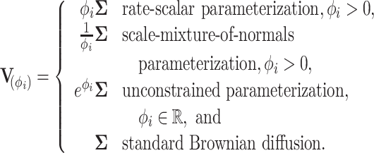
where the matrix-valued function characterizes the branch-specific multivariate normal (MVN) increment that defines the diffusion process. We parameterize this function in terms of an unknown positive-definite matrix that describes the covariation between trait dimensions after controlling for shared evolutionary history and an unknown branch-rate multiplier . Typical choices include

(2)

To complete the RRW model specification, we adopt a prior density on the unobserved trait at the parentless root node,

(3)

with prior mean and sample size .

Letting and the observed data at the tips, we are interested in learning about the posterior

(4)

where is an unknown parameter characterizing our prior on and represents parameters of a molecular sequence substitution model for the evolution of aligned molecular sequence data . Note that we follow usual convention (Cybis et al. 2015) and assume that and are conditionally independent given . We follow the example of Lemey et al. (2010) and place a log-normal prior distribution on with mean and standard deviation . We further assume an exponential prior on with mean . In the examples that follow, we place one of two priors on the covariance structure . In our first example, we study the West Nile virus and follow the original modeling assumptions of Pybus et al. (2012). We assign a Wishart conjugate prior with scale matrix and degrees of freedom to . In our second example, we study correlation between mammalian life history traits and employ a more general “separation strategy” whereby is separated into a correlation matrix and diagonal variance matrix (Barnard et al. 2000; Zhang et al. 2006; Caetano and Harmon 2019). We specify the eponymous “LKJ” prior (Lewandowski et al. 2009) on the correlation matrix and assign the diagonal of marginal variances a log-normal distribution with mean and standard deviation of . The LKJ prior is uniform over the space of positive-definite correlation matrices, and this is favorable for our purpose of comparing correlation estimates under contrasting models. Efficient application of the LKJ prior in phylogenetics is well described by Zhang et al. (2019).

We use MCMC integration to approximate this posterior using a random-scan Metropolis-within-Gibbs approach (Levine and Casella 2006; Liu 2008). One cycle of this scheme consists of sampling and then via

(5a)

(5b)

(5c)

(5d)

where update (5d) is unnecessary when is fixed, otherwise efficient sampling from the density is well described elsewhere, see for example Suchard et al. (2018). Updates (5b) and (5c) are straightforward due to the conjugate priors chosen in our model. We turn our focus to the remaining component of our scheme, namely sampling from .

Hamiltonian Monte Carlo

We wish to sample jointly to avoid potentially high autocorrelation in the resulting MCMC chain. To this end, we propose using HMC and begin with a brief description of how HMC maps sampling from a probability distribution to simulating a physical system. In classical mechanics, the Hamiltonian is the sum of the kinetic and potential energy in a closed system. To build the connection, we introduce auxiliary momentum variable and write our Hamiltonian,

(6)

where the mass matrix weights our momentum variables. The canonical distribution from statistical mechanics relates the joint density of state variables and to the energy in a system via the relationship,

(7)

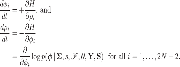
Substituting our Hamiltonian into (7), we observe that and are independent and recognize the marginal density of to be MVN. To start the HMC algorithm, we first sample from this marginal density. Then by differentiating , we generate Hamilton’s equations of motion,

(8)

We can use the resulting vector field in conjunction with a variety of numerical integration techniques to propose new states of for our MCMC chain. Consistent with typical construction (Neal 2011), we use the leapfrog method for numerical integration, where we follow the trajectory of for a half-step before updating . For a full discussion of HMC, see Neal (2011). Importantly, Hamilton’s equations elicit a need to calculate the gradient at each chain step to traverse phase space and gradient computation can be costly.

Gradient of Trait Data Log-likelihood

A practical HMC sampler demands efficient calculation of . Differentiating the logarithm of (5a), we obtain

(9)

Our log-normal prior choice for renders evaluating the second term in Equation (9) trivial. Here, we develop a general recursive algorithm for calculating . To facilitate this development, consider splitting into two disjoint sets relative to any node in . We define as the observed data descendant of node and as the observed data “above” (or not descendent of) node . For clarity, see Figure 1.

Figure 1.

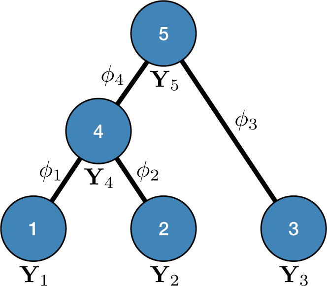
Example tree with tips. Assume trait data are fully observed for . We write and to denote the observed data below and above node respectively. Specifically, while . Partial likelihoods and .

In the following, we drop the dependence of the log-likelihood on , and for notational convenience. To begin,

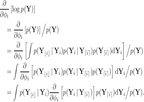(10)

The last equality above follows from the fact that is associated only with the branch above node . Therefore, when we condition on , is independent of . Similarly, evolves independent of . To proceed with the differential above, we use the fact that follows a MVN distribution with as of yet undetermined mean and precision (see Section 6.1 for a detailed derivation). We extract the middle term from Equation (10) and find

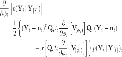(11)

using the differential properties

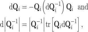(12)

found in, for example, Petersen and Pedersen (2012).

To simplify notation, we let function

(13)

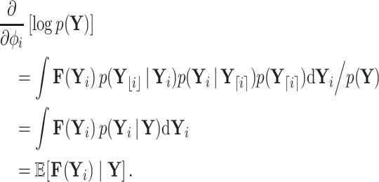
where and . Substituting Equation (13) back into Equation (10), we observe that

(14)

When is fully observed (typically ), this expectation collapses to the direct evaluation of . When or if is partially observed for , we require . From Bayes’ theorem, . Partial likelihood is proportional to a MVN density characterized by computable mean and precision (Pybus et al. 2012). Using this fact, becomes MVN with mean and variance When tip is partially observed, we partition into its unobserved and observed entries. Using properties of the conditional MVN, becomes degenerate with mean

(15)

and variance

(16)

Finally, for both partially and completely unobserved cases above,

(17)

Equation (17) provides a recipe to compute using the means and precisions that characterize partial data likelihoods and .

Tree Traversals

We introduce post- and preorder tree traversals to recursively calculate all partial data likelihood means and precisions in computational complexity that scales linearly with . To begin, let nodes and be daughters of node . Following Hassler et al. 2020, let for be a diagonal matrix with indicator elements that take value if is observed and if not. For the postorder traversal,

(18)

with postorder mean and precision . For in postorder, we build the precision via

(19)

with the definition that and

(20)

where the pseudo-inverse, defined and developed by Bastide et al. 2018 and Hassler et al. 2020, is described in Appendix (6.2). At the tips, we build the mean where is the elementwise dot product, and for the internal nodes, is a solution to

(21)

For a proof of these post-order updates, see Hassler et al. (2020) (Supplementary Material available on Dryad at http://dx.doi.org/10.5068/dryad.D1BM1R).

To compute , we traverse the tree in preorder fashion according to our generalized version of the recursive algorithm proposed by Cybis et al. (2015). See Section 6.1 for a derivation of our generalized preorder update. For the preorder traversal,

(22)

For looking down the tree, we update our preorder precision,

(23)

at each node where

(24)

We also keep track of the preorder mean at each node via

(25)

Both traversals visit each node exactly once and perform a matrix inversion as their most costly operation, providing an algorithm. However, as we observe in Equation (2), generally . In this case, we can further reduce the computational complexity to by factoring out . Instead of inverting at each step, we only need to invert at most once per likelihood or gradient evaluation.

Results

West Nile Virus

West Nile virus (WNV) is responsible for more than 1500 deaths and caused over 700,000 illnesses since first reported in North America in 1999. The virus typically spreads via mosquito bites; however, the primary host is birds. First identified in New York City, WNV spread to the Pacific coast by 2003 and reached south into Argentina by 2005 (Petersen et al. 2013). We examine whole aligned viral genomes (11,029 nt) and geographic data on cases of WNV collected between 1999 and 2007 (Pybus et al. 2012). In cases where only the year of sampling is known, we set the sampling date to the midpoint of that year. Previous authors have recorded latitude and longitude geographic sampling information by converting zip code locations using ZIPList5. For 27 of the specimens, only the US or Mexican state of discovery is known and so we have augmented sampling data with the coordinates of the centroid of the state (Pybus et al. 2012).

Here, we study the simultaneous evolution and dispersal of WNV as it spreads across North America, following the modeling choices of Pybus et al. (2012). We define geographic location as our trait of interest within a RRW and infer rates using our new HMC method. In two separate inference scenarios, we compare the computational efficiency of our method to the random-scan UMH approach employed by Pybus et al. (2012). The UMH kernel proposes new branch-rate multipliers individually by randomly scaling up or down the current . Under the UMH, all dimensions of share the same adaptable tuning constant that controls the scaling range. Additionally, we compare our method to a less naive univariable proposal that provides each dimension of its own adaptable tuning constant. We term this transition kernel multiple Metropolis–Hastings (MMH).

To begin, we set up a RRW model with log-normal prior on rates with mean and standard deviation and use a general time-reversible (GTR) + substitution model with a log-normal relaxed molecular clock. We use the UMH transition kernel to run a 250 million state MCMC chain simulation to obtain posterior mean estimates of and . 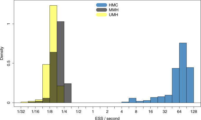In scenario (a), we use these fixed model parameters and a topology drawn from the posterior to strictly sample using HMC and univariable transition kernels. Under this fixed analysis, we run our HMC-based chain for 1 million states and UMH/MMH-based chains for 150 million states. We use effective sample size (ESS) of the posterior samples for all divided by computational runtime to evaluate the performance of each MCMC approach and report densities of ESS/second across all branches in Figure (2). ESS/second is averaged across five runs each with uniform (0–10) random initial branch-rate multipliers. The median ESS/second across is , and for the HMC, MMH, and UMH transition kernels, respectively. This demonstrates an over -fold speed increase. Additionally, the minimum ESS/s is with HMC, with MMH, and with UMH, exhibiting a -fold speed-up for the “least well” explored .

Figure 2.

Comparing computational efficiency of Hamiltonian Monte Carlo (HMC) to univariable Metropolis–Hastings (UMH) and multiple Metropolis–Hastings (MMH) transition kernels through effective sample size (ESS) per unit time in West Nile virus (WNV) phylogeography.

In scenario (b), we use a random starting tree and jointly estimate all parameters (, , and ) of the full posterior (4). Since branch-specific are no longer identifiable when is random, we compare square jump distance across all between samples from the posterior under both MCMC regimes to compare efficiency. We run HMC chains for 22.5 million states so that we are sampling from the posterior distribution of all parameters, and we save the state of BEAST. Subsequently, we run both HMC and UMH chains from the same saved states and compute lag-7 square jump distance to adjust for the relative weight of the transition kernel in the full analysis. Since the UMH sampler updates only one branch-rate multiplier at a time, we compare square jump distance between samples of our HMC chain with samples from the UMH chain that are lagged (i.e., ) farther apart. We run each MCMC simulation until we obtain 5000 samples from the posterior and report the average median across five separate runs. In this comparison, we find that the average median square jump distances from five separate runs is and for the HMC and UMH chains, respectively.

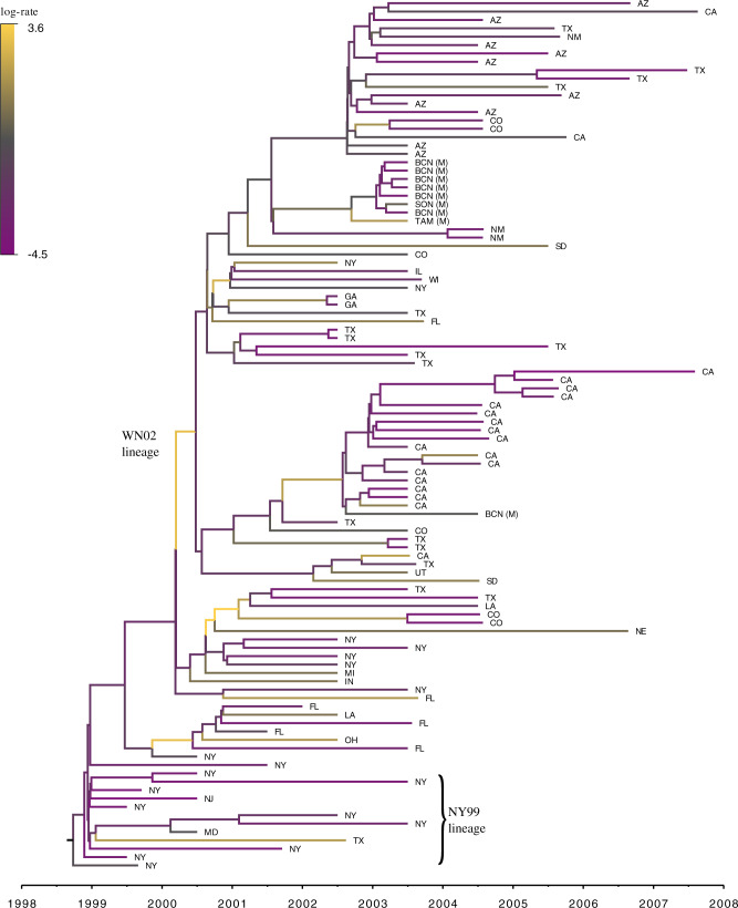
In Figure (3), we report the MCC tree, obtained from applying HMC to the RRW model as described in scenario (b), where substitution rate variation is accounted for by the molecular clock model. The branch with the highest posterior dispersal rate starts the WN02 lineage identified by Gray et al. (2010). The clade of New York isolates sampled in 1999, however, maintains a much slower dispersal rate. We obtain results under this joint inference test by running an MCMC chain until we observe ESS for all parameters of interest, namely the height of the tree, substitution model parameters, the diffusion matrix , prior standard deviation and 90% of the dimensions of . We choose only 90% because many dimensions of exhibit multi-modality and therefore experience poor mixing when the tree is random. Under the UMH transition kernel this analysis takes approximately 45.8 h. Under HMC, this analysis completes in 7.1 h, a 6.4-fold speed-up. We report average times across five runs. The ESS-limiting parameters in each case are the multi-modal branch-rate multipliers.

Figure 3.

Maximum clade credibility (MCC) tree resulting from Hamiltonian Monte Carlo (HMC) inference under phylogeographic relaxed random walk (RRW) of West Nile virus. We color branches by posterior mean branch-rate parameters . Tips are labeled according to the US or Mexican state of origin.

Mammalian Life History

Life history theory aims to explain how traits such as adult body mass, litter size, and lifespan evolve to optimize reproductive success (Stearns 2000). Life history theory finds important applications in determining a species’ fecundity and predicting extinction risk in response to changing environmental stimuli (Fritz et al. 2009; Pacifici et al. 2017; de Silva and Leimgruber 2019), but due to the sparseness of much life history data, it is essential to understand how traits covary to make meaningful predictions (Santini et al. 2016). To determine which traits covary, comparative mammalian life history studies posit a ‘fast-slow’ continuum, claiming small mammals are typically “fast,” characterized by early maturation, large litters, and shorter lifespans, while larger mammals are typically “slow” and present contrasting characteristics (Oli 2004; Millar and Zammuto 1983). Under this framework, certain traits such as gestation length, weaning age, and body mass are predicted to be positively correlated, but reported estimates of positive correlation from data may be artifacts of the restrictive assumptions of strict Brownian diffusion modeling. Here, we re-evaluate this claim by comparing inferred trait correlation under the strict Brownian diffusion model with estimates under the RRW of trait evolution made tractable through HMC sampling.

Under the RRW, we infer correlation between five life history traits from the PanTHERIA data set (Jones et al. 2009), namely body mass, litter size, gestation length, weaning age, and litter frequency across mammalian species related by the fixed supertree of Fritz et al. (2009). To obtain this subset of the supertree, we only consider taxa for which at least one of these five traits is observed. We take the intersection of this set of taxa with those in the fixed supertree of Fritz et al. (2009) and prune all other observations from the tree. We log-transform and standardize the trait measurements and subsequently estimate posterior mean correlations between each pair of traits under the RRW using an HMC-based chain for 300,000 states. We model diffusion using the rate-scalar parameterization of noted in equation (2). This modeling choice assumes that all taxa share a common correlation structure across the tree. To gauge the effect of a heterogeneous diffusion process on the correlation between traits, we also make inference using the strict Brownian diffusion model where the are all identically . Here, we perform MCMC inference on the diffusion matrix for 50,000 states. Under the RRW, we find the variance in body mass is with 95% high posterior density (HPD) interval , gestation length is , weaning age is , litter frequency is , and litter size is . We report posterior mean estimates of correlation between each pair of traits under both the RRW and strict Brownian diffusion in Figure (4).

Figure 4.

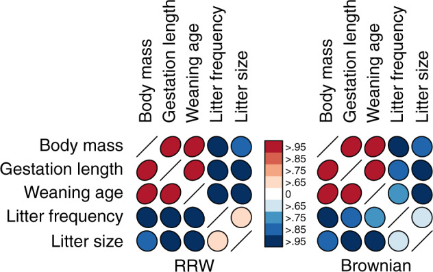
Posterior mean correlation between mammalian life history traits under the RRW and strict Brownian diffusion model. Shape of ellipse indicates strength and sign of correlation, while colors indicate the posterior probability that the correlation is positive (red) or negative (blue).

In most cases, the RRW reassuringly confirms analysis under the more limited model. However, in some cases our confidence in the sign of the correlation differs between models and in one instance the sign of the posterior mean correlation disagrees. Under the RRW, we observe positive posterior mean correlation of between litter frequency and litter size with posterior odds ratio that the correlation is positive. Under the strict Brownian diffusion model we observe a negative posterior mean correlation of with posterior odds ratio of being negative, indicating slightly weaker belief in the correlation’s sign under the strict model.

Discussion

Previous MCMC techniques to investigate trait evolution under the RRW model scale poorly with large data sets. Specifically, the UMH transition kernel is ineffective for sampling correlated, high-dimensional parameter space. We provide a remedy by using an HMC transition kernel to sample all branch-rate multipliers simultaneously. To improve the speed of HMC, we derive an algorithm for calculating the gradient of the trait data log-likelihood. This gradient calculation achieves computational speed, a vast improvement compared to both numerical and pruning methods for calculating the gradient that typically require .

We observe over 300-fold speed-up when comparing, on a fixed phylogeny, our HMC transition kernel to both MMH and UMH in the spread of the WNV across North America in the early 2000s. Additionally, we note here that HMC on the branch-rate multipliers also improves sampling of hyperparameter as suggested by Equation (5c). HMC offers an over 6-fold speed increase in total run-time when jointly estimating parameters of the RRW, substitution model, and phylogeny. The resulting MCC tree reveals that the largest dispersal rate precedes the most recent common ancestor of the WN02 lineage. Subsequently, the dispersal rates slow down through the WN02 clade. This suggests that this clade developed after some rapid geographic displacement. Interestingly, the appearance of smaller branch-rate multipliers within the WN02 lineage is consistent with the slowing speed of sequence evolution as described in Snapinn et al. (2007).

As exhibited in Figure (2), ESS from posterior sampling accumulates at variable speed across the branches of the tree. To further improve the sampling of our HMC algorithm, one might use an approximation of the posterior covariance of for the mass matrix to appropriately weight momentum updates in the HMC algorithm (Neal 2011). Possible approximations include the Hessian of the log-posterior (a local approximation of the curvature of branch-rate multiplier space) or the sample variance across each dimension. An important consideration in choosing an appropriate is whether one is studying under a fixed or random phylogeny . Since varying in the posterior often creates multimodal distributions of , local approximations such as the Hessian may be of limited assistance in such cases.

We show in our application to mammalian life history that our computationally efficient HMC algorithm imbues the RRW model with the ability to handle large trees with thousands of taxa. By applying the RRW model to this massive example, we confirm that large mammals have “slower” life history characteristics, exhibited by the positive correlation among body mass, gestation length, and weaning age, while smaller mammals scale in the opposite manner and tend to have high litter frequency and size, see Figure (4). The posterior mean correlation between litter frequency and litter size changes sign under each model, but with low posterior probability reflecting a lack of correlation between these traits. Note that the diffusion variance choices listed in Equation (2) all assume that the branch-rate multipliers scale each trait equally. Future modeling work could relax this assumption by letting each element of the diffusion matrix be a function of the branch-rate multipliers. Importantly, our method allows us to obtain posterior estimates for the correlation matrix in 32 h while the previous UMH method fails to estimate the correlation matrix and branch-rate multipliers with greater than 200 ESS after 10 days.

In a time where biological data are more prolific than ever, scalable approaches to complex models of evolution such as the RRW prove increasingly useful in a variety of applications. From spatial epidemiology where determining the dispersal rate of an infectious disease is crucial, to evolutionary ecology where understanding life history can provide insight into declining animal populations, the analysis of data is becoming a bottleneck to the scientific process and the need for computationally faster approaches stands evident. We hope that this work will serve to improve the speed of such analyses. We make all BEAST XML files used in this work publicly available at http://github.com/suchard-group/RRW_at_scale.

 

Appendices

Preorder Partial Likelihood

Here, we derive a generalized version of the preorder recursive algorithm proposed by Cybis et al. (2015) to compute for all in . We begin with the law of total probability,

(A1)

for node with parent and sibling . Recalling that

(A2)

we identify Equation (A1) as a recursive expression whose solution has the form

(A3)

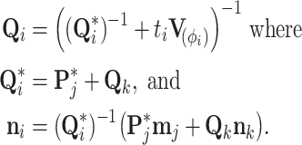
with presently undetermined preorder mean and preorder precision .

We unravel these quantities by first identifying that and set and . Then proceeding in preorder fashion for

(A4)

Pseudo-inverse

The pseudo-inverse used in the post-order tree traversal and defined by (Bastide et al. 2018) and (Hassler et al. 2020) is an operation for inverting precision and variance matrices with diagonal entries that take the value . To invert a diagonal precision matrix, with entries and , we define and . To invert the variance matrix , we invert the block matrix of observed trait covariation and invert the remaining diagonal elements using the convention that .

Supplementary Material

Data available from the Dryad Digital Repository: http://dx.doi.org/10.5068/dryad.D1BM1R.

Funding

This work was supported by the European Research Council under the European Union’s Horizon 2020 research and innovation programme [725422 - ReservoirDOCS]; The Artic Network from the Wellcome Trust [206298/Z/17/Z]; National Science Foundation [DMS 1264153]; National Institutes of Health [R01 AI107034, U19 AI135995, and T32 GM008185 to A.A.F.]; and Research Foundation – Flanders [‘Fonds voor Wetenschappelijk Onderzoek – Vlaanderen’, G066215N, G0D5117N, and G0B9317N] to P.L.

References

- Barnard J., McCulloch R., and Meng X.-L.. 2000. Modeling covariance matrices in terms of standard deviations and correlations, with application to shrinkage. Stat. Sin. 10:1281–1311. [Google Scholar]
- Bastide, P., Ané, Robin S., and Mariadassou M.. 2018. Inference of adaptive shifts for multivariate correlated traits. Syst. Biol. 67:662–680. [DOI] [PubMed] [Google Scholar]
- Bedford T., Suchard M.A., Lemey P., Dudas G., Gregory V., Hay A.J., McCauley J. W., Russell C.A., Smith D.J., and Rambaut A.. 2014. Integrating influenza antigenic dynamics with molecular evolution. eLife 3:e01914. [DOI] [PMC free article] [PubMed] [Google Scholar]
- Biek R., Henderson J.C., Waller L.A., Rupprecht C.E., and Real L.A.. 2007. A high-resolution genetic signature of demographic and spatial expansion in epizootic rabies virus. Proc. Natl. Acad. Sci. USA, 104:7993–7998. [DOI] [PMC free article] [PubMed] [Google Scholar]
- Bryant D., Galtier N., and Poursat M.-A.. 2005. Likelihood calculation in molecular phylogenetics. In: Gascuel O., editor. Mathematics of evolution and phylogeny. Oxford: Oxford University Press. p. 33–62. [Google Scholar]
- Caetano D.S., Harmon L.J.. 2019. Estimating correlated rates of trait evolution with uncertainty. Syst. Biol. 68:412–429. [DOI] [PubMed] [Google Scholar]
- Cybis G.B., Sinsheimer J.S., Bedford T., Mather A.E., Lemey P., and Suchard M. A.. 2015. Assessing phenotypic correlation through the multivariate phylogenetic latent liability model. Ann. Appl. Stat. 9:969. [DOI] [PMC free article] [PubMed] [Google Scholar]
- de Silva S. and Leimgruber P.. 2019. Demographic tipping points as early indicators of vulnerability for slow-breeding megafaunal populations. Front. Ecol. Evol. 7:171. [Google Scholar]
- Faria N.R., Rambaut A., Suchard M.A., Baele G., Bedford T., Ward M.J., Tatem A.J., Sousa J.D., Arinaminpathy N., Pépin J., Posada D., Peeters M., Pybus O.G., Lemey P.. 2014. The early spread and epidemic ignition of HIV-1 in human populations. Science 346:56–61. [DOI] [PMC free article] [PubMed] [Google Scholar]
- Felsenstein J. 1981. Evolutionary trees from DNA sequences: a maximum likelihood approach. J. Mol. Evol. 17:368–376. [DOI] [PubMed] [Google Scholar]
- Felsenstein J. 1985. Phylogenies and the comparative method. Am. Nat. 125:1–15. [Google Scholar]
- Fritz S.A., Bininda-Emonds O.R. and Purvis A.. 2009. Geographical variation in predictors of mammalian extinction risk: big is bad, but only in the tropics. Ecol. Lett. 12:538–549. [DOI] [PubMed] [Google Scholar]
- Gray R., Veras N., Santos L., and Salemi M.. 2010. Evolutionary characterization of the West Nile virus complete genome. Mol. Phylogenet. Evol. 56:195–200. [DOI] [PubMed] [Google Scholar]
- Hassler G., Tolkoff M.R., Allen W.L., Ho L.S.T., Lemey P., Suchard M.A.. Forthcoming 2020. Inferring phenotypic trait evolution on large trees with many incomplete measurements. J. Am. Stat. Assoc. [DOI] [PMC free article] [PubMed] [Google Scholar]
- Hastings W.K. 1970. Monte Carlo sampling methods using Markov chains and their applications. Biometrika 57:97–109. [Google Scholar]
- Ives A.R., Garland T. Jr.. 2009. Phylogenetic logistic regression for binary dependent variables. Syst. Biol. 59:9–26. [DOI] [PubMed] [Google Scholar]
- Jones K.E., Bielby J., Cardillo M., Fritz S.A., O’Dell J., Orme C.D.L., Safi K., Sechrest W., Boakes E.H., Carbone C., et al. 2009. PanTHERIA: a species-level database of life history, ecology, and geography of extant and recently extinct mammals. Ecology 90:2648–2648. [Google Scholar]
- Lemey P., Rambaut A., Welch J.J., and Suchard M.A.. 2010. Phylogeography takes a relaxed random walk in continuous space and time. Mol. Biol. Evol. 27:1877–1885. [DOI] [PMC free article] [PubMed] [Google Scholar]
- Levine R.A., Casella G.. 2006. Optimizing random scan Gibbs samplers. J. Multivar. Anal. 97:2071–2100. [Google Scholar]
- Lewandowski D., Kurowicka D., and Joe H.. 2009. Generating random correlation matrices based on vines and extended onion method. J. Multivar. Anal. 100:1989–2001. [Google Scholar]
- Liu J.S. 2008. Monte Carlo strategies in scientific computing. New York: Springer Science & Business Media (Springer Series in Statistics). [Google Scholar]
- Millar J.S., Zammuto R.M.. 1983. Life histories of mammals: an analysis of life tables. Ecology 64:631–635. [Google Scholar]
- Neal R.M. 2011. MCMC using Hamiltonian dynamics. In: Brooks S., Gelman A., Jones G.L., Meng X.-L., editors. Handbook of Markov chain Monte Carlo, vol. 2. New York, NY, CRC Press. [Google Scholar]
- Oli M.K. 2004. The fast–slow continuum and mammalian life-history patterns: an empirical evaluation. Basic Appl. Ecol. 5:449–463. [Google Scholar]
- Pacifici M., Visconti P., Butchart S.H., Watson J.E., Cassola F.M., and Rondinini C.. 2017. Species’ traits influenced their response to recent climate change. Nat. Clim. Change 7:205. [Google Scholar]
- Petersen K.B., Pedersen M.S.. 2012. The matrix cookbook, vol. 7. Lyngby, Denmark: Technical University of Denmark. [Google Scholar]
- Petersen L.R., Brault A.C., and Nasci R.S.. 2013. West Nile virus: review of the literature. J. Am. Med. Assoc. 310:308–315. [DOI] [PMC free article] [PubMed] [Google Scholar]
- Pybus O.G., Suchard M.A., Lemey P., Bernardin F.J., Rambaut A., Crawford F.W., Gray R.R., Arinaminpathy N., Stramer S.L., Busch M.P., et al. 2012. Unifying the spatial epidemiology and molecular evolution of emerging epidemics. Proc. Natl. Acad. Sci. USA 109:15066–15071. [DOI] [PMC free article] [PubMed] [Google Scholar]
- Santini L., Cornulier T., Bullock J.M., Palmer S.C., White S.M., Hodgson, J.A., Bocedi G., and Travis J.M.. 2016. A trait-based approach for predicting species responses to environmental change from sparse data: how well might terrestrial mammals track climate change? Global Change Biol. 22:2415–2424. [DOI] [PubMed] [Google Scholar]
- Schluter D., Price T., Mooers A.Ø., and Ludwig D.. 1997. Likelihood of ancestor states in adaptive radiation. Evolution 51:1699–1711. [DOI] [PubMed] [Google Scholar]
- Snapinn K.W., Holmes E.C., Young D.S., Bernard K.A., Kramer L.D., and Ebel G.D.. 2007. Declining growth rate of West Nile virus in North America. J. Virol. 81:2531–2534. [DOI] [PMC free article] [PubMed] [Google Scholar]
- Stearns S.C. 2000. Life history evolution: successes, limitations, and prospects. Naturwissenschaften 87:476–486. [DOI] [PubMed] [Google Scholar]
- Suchard M.A., Lemey P., Baele G., Ayres D.L., Drummond A.J., and Rambaut A.. 2018. Bayesian phylogenetic and phylodynamic data integration using BEAST 1.10. Virus Evol. 4:vey016. [DOI] [PMC free article] [PubMed] [Google Scholar]
- Zhang X., Boscardin W.J., and Belin T.R.. 2006. Sampling correlation matrices in Bayesian models with correlated latent variables. J. Comput. Graph. Stat. 15:880–896. [Google Scholar]
- Zhang Z., Nishimura A., Bastide P., Ji X., Payne R.P., Goulder P., Lemey P., and Suchard M.A.. Forthcoming 2019. Large-scale inference of correlation among mixed-type biological traits with phylogenetic multivariate probit models. Ann. Appl. Stat. [Google Scholar]