Integrated spatial genomics reveals global architecture of single nuclei

Abstract

Identifying the relationships between chromosome structures, nuclear bodies, chromatin states, and gene expression is an overarching goal of nuclear organization studies^1–4. Because individual cells appear to be highly variable at all these levels⁵, it is essential to map different modalities in the same cells. Here, we report the imaging of 3,660 chromosomal loci in single mouse embryonic stem cells (mESCs) by DNA seqFISH+, along with 17 chromatin marks and subnuclear structures by sequential immunofluorescence (IF) and the expression profile of 70 RNAs. We found many loci were invariantly associated with IF marks in single mESCs. These loci form “fixed points” in the nuclear organizations in single cells and often appear on the surfaces of nuclear bodies and zones defined by combinatorial chromatin marks. Furthermore, highly expressed genes appear to be pre-positioned to active nuclear zones, independent of bursting dynamics in single cells. Our analysis also uncovered several distinct mESCs subpopulations with characteristic combinatorial chromatin states. Using clonal analysis, we show that the global levels of some chromatin marks, such as H3K27me3 and macroH2A1 (mH2A1), are heritable over at least 3–4 generations, whereas other marks fluctuate on a faster time scale. This seqFISH+ based spatial multimodal approach can be used to explore nuclear organization and cell states in diverse biological systems.

The main approaches to examine nuclear organization have been sequencing based genomics and microscopy^1,3. Genomics approaches, such as Hi-C⁶ and SPRITE⁷, have been powerful in mapping interactions between chromosomes genome-wide and have been scaled down to the single cell level^1,3. However, reconstructing 3D structures from the measured interactions relies on computational models, and it is difficult to integrate multiple modalities of measurements^2,4 including chromosome structures in the same cells. On the other hand, microscopy-based methods can directly image chromosomes and nuclear bodies^1,3. Recent methods^8–15 using Oligopaint¹⁶ and sequential DNA fluorescence in situ hybridization (DNA FISH) have imaged many DNA loci in single cells. These studies have shown that chromosome organization is highly heterogeneous at the single cell level^8–15, such as the variability of chromosome folding even between two alleles in single cells^8–10,12,15. To further discover organizational principles at the single cell level, we need integrated tools to image chromosomes as well as nuclear bodies and chromatin marks that are aligned precisely in the same cells.

DNA seqFISH+ imaging in single cell

Building upon seqFISH^17–21 and other multiplexed FISH methods^{8–11,13,16,22}, we now developed DNA seqFISH+ to target 3,660 loci in single mouse embryonic stem cells (mESCs) (Fig. 1, Extended Data Fig. 1, 2, Supplementary Table 1, 2). In two of the fluorescent channels, we used seqFISH+ coding scheme (see Methods) to target 1,267 loci approximately 2 megabases (Mb) apart (Fig. 1b, c) and 1,193 loci at 5’ end of genes, respectively. Together these two channels labeled 2,460 loci spaced approximately 1 Mb apart across the whole genome. At the same time, the third fluorescent channel targeted 60 consecutive loci at 25 kb resolution on each of the 20 chromosomes for an additional 1,200 loci (Fig. 1b, d). These approaches allowed us to examine nuclei at both 1 Mb resolution for the entire genome, and 25 kb resolution for 20 distinct regions that are at least 1.5 Mb in size (Fig. 1e).

Figure 1. DNA seqFISH+ imaging of chromosomes.

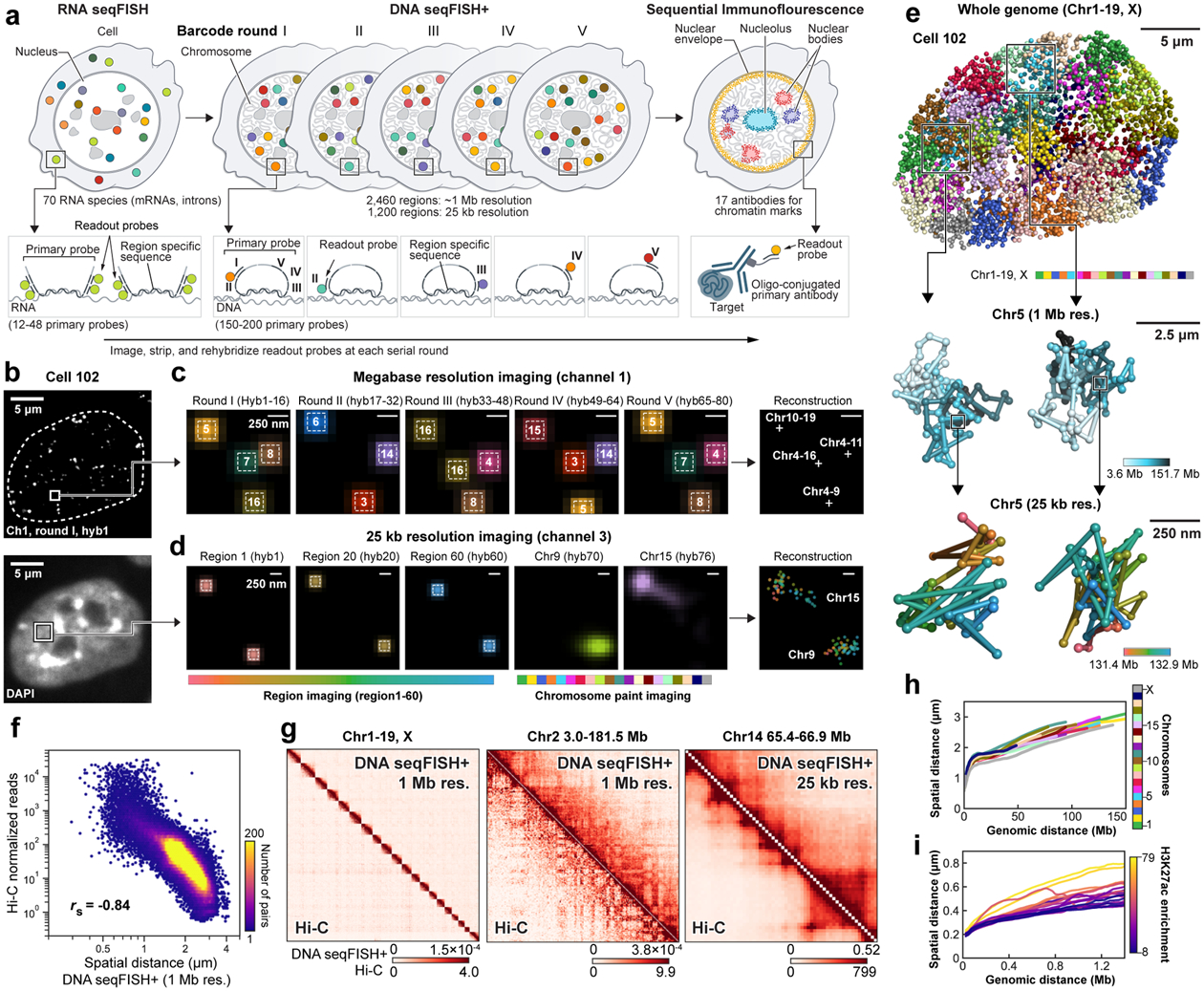
a, Schematic for DNA seqFISH+ combined with RNA seqFISH and sequential immunofluorescence (IF) (see Methods). b, Example images for DNA seqFISH+ in a mESC. Top, DNA seqFISH+ image from one round of hybridization at a single z section. Bottom, DAPI image from the same z section of the cell. c, Zoomed-in view of the boxed region in b through five rounds of barcoding. Images from 16 serial hybridizations are collapsed into a single composite image, corresponding to one barcoding round. White boxes on pseudocolor spots indicate identified barcodes. d, Zoomed-in view of the boxed region in b through 60 rounds targeting adjacent regions at 25 kb resolution followed by 20 rounds of chromosome painting in channel 3. Scalebars represent 250 nm in zoomed-in images. e, 3D image of a single mESC nucleus. Top, individual chromosomes labeled in different colors. Middle, two alleles of chromosome 5 colored based on chromosome coordinates. Bottom, two alleles of 1.5 Mb regions in chromosome 5 with 25 kb resolution. f, Comparison of median spatial distance between pairs of intra-chromosomal loci by DNA seqFISH+ and Hi-C²³ frequencies. Spearman correlation coefficient of −0.84 computed from n = 146,741 unique intra-chromosomal pairs in autosomes. g, Concordance between DNA seqFISH+ (upper right) and Hi-C²³ maps (lower left) at different length scales. h, i, Physical distance as a function of genomic distance Mb resolution in h and 25 kb resolution in i. Median spatial distances per genomic bin are shown. H3K27ac enrichments of the entire region are obtained from ChIP-seq²⁴ in i. n = 446 cells in two biological replicates in f-i.

DNA seqFISH+ detected 5,616.5 ± 1,551.4 (median ± standard deviation) dots per cell in total with 1 Mb and 25 kb resolution data (Extended Data Fig. 2h–k) in 446 cells from two biological replicates. This corresponds to an estimated detection efficiency of at least 50% in the diploid genome considering the cell cycle phases (see Methods). The false positive dots, as determined by the barcodes unused in the codebook, were detected at 14.0 ± 7.4 per cell (median ± standard deviation).

Imaged chromosomes in single cells showed clear physical territories for individual chromosomes and have variable structures amongst cells and chromosomes (Fig. 1e, Extended Data Fig. 3, 4). The DNA seqFISH+ measurements were highly reproducible between biological replicates (Extended Data Fig. 2l, m), and agreed with population Hi-C²³ and SPRITE data⁷ (Fig. 1f, g, Extended Data Fig. 3a–g). The genomic versus physical distance scaling relationships for each chromosome differ amongst the chromosomes at 1 Mb resolution as well as at 25 kb resolution (Fig. 1h, i ,Extended Data Fig. 4c, d), showing regions with low H3K27ac marks²⁴ tend to have more compact spatial organization (Fig. 1i) possibly due to different underlying epigenetic states²⁵.

Integrated measurements in single cells

We integrated our analysis of the genome (DNA seqFISH+) with the transcripts (RNA seqFISH) as well as histone modifications and subnuclear structures (immunofluorescence (IF)) (Fig. 1a and Extended Data Fig. 1a). 17 primary antibodies targeting nuclear lamina²⁶, nuclear speckle²⁷, nucleolus²⁸ and active and repressive histone modification markers²⁹ were conjugated with DNA oligonucleotides (oligos)^30,31, allowing the selective readout of individual primary antibodies with fluorescently labeled readout probes (Fig. 2a and Extended Data Fig. 1a, 2f, g, 5). These antibodies and RNA FISH probes for 70 mRNA and intron species were hybridized in the same cells as the DNA seqFISH+ probes. Additionally, 4 repetitive regions that relate to nuclear organization^32,33 were sequentially imaged with DNA FISH (Extended Data Fig. 5a).

Figure 2. DNA seqFISH+ combined with sequential IF reveals invariant features.

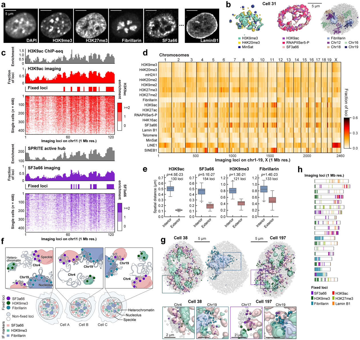
a, Images for DAPI and immuno- staining in a mESC nucleus. Scale bars, 5 μm. b, 3D images for sequential IF and DNA seqFISH+ in the same cell in a. IF pixels with intensity Z-score values above 2 are shown (for other markers and cells, see Extended Data Fig. 5c, d). c, Comparison of “chromatin profiles,” the fraction of loci found within 300 nm of H3K9ac and SF3a66 exteriors with corresponding reference profiles^7,24 (top) and the single cell spatial proximity profiles of 446 single cells sorted by enrichment (bottom). Fixed loci were determined by Z-score above 2 from loci in all chromosomes. d, Heatmap showing fraction of DNA loci within 300 nm from interiors of IF markers and repetitive elements at 1 Mb resolution (see Extended Data Fig. 5g for 25 kb resolution data). e, Comparison of median distance of fixed loci to IF interior and exterior voxels (see Methods). p values were calculated with a two-sided Wilcoxon’s signed-rank sum test. The boxplots represent the median, interquartile ranges, whiskers within 1.5 times the interquartile range, and outliers. f, Illustration showing chromosome 4 with fixed loci for SF3a66 and H3K9me3, while chromosome 19 contains fixed loci for SF3a66 and Fibrillarin. g, Representative 3D images for fixed loci and IF markers. For IF marks, pixels with intensity Z-score values above 2 for each IF mark were shown. Bottom panels show zoomed-in views of individual chromosomes (chr4, 17 or 19) and contain all 3 markers (SF3a66, H3K9me3 and Fibrillarin; for other chromosomes, markers and cells, see Extended Data Fig. 6h, i). h, Fixed loci distribution along the chromosome coordinates for all chromosomes. Each bin represents an imaging locus by 1 Mb resolution DNA seqFISH+ (n = 2,460 loci). n = 446 cells from 2 biological replicates for c-h.

We extensively optimized the combined protocols (see Methods and Extended Data Fig. 1a, 2a–g) to profile these different modalities and accurately align between IF and DNA FISH images for over 130 rounds of hybridizations on an automated confocal microscope.

Repressive histone marks (e.g. H3K9me3, H4K20me3) colocalized with DAPI rich regions and minor satellite DNA (MinSat) corresponded to pericentromeric and centromeric heterochromatin^32,33 (Fig. 2b left, Extended Data Fig. 5d). Immunofluorescence of RNA polymerase II (RNAPIISer5-P) and active marks (H3K9ac, H3K27ac) localized to the periphery of nuclear speckles (SF3a66) (Fig. 2b middle, Extended Data Fig. 5d) and were excluded from both heterochromatic regions and the nuclear lamina (Extended Data Fig. 5d), consistent with the localization patterns reported in the literature^27,34. We also note that chromosomes 12, 16, 18 and 19, which contain rDNA arrays⁷, showed significant association with the nucleoli (Fig. 2b right, Extended Data Fig. 5d).

Fixed loci are consistent in single cells

From the integrated multiplexed IF and DNA seqFISH+ data, we systematically calculated the physical distances between each DNA locus and the nearest “hot” IF voxel, defined by two standard deviations above the mean value for each IF marker (Extended Data Fig. 5b, c). Because many IF markers form discrete globules in the nucleus, we also calculated the distance of each DNA loci to the exterior of IF nuclear bodies (see Methods), and confirmed both metrics are highly correlated (Extended Data Fig. 5e, f).

We can generate a “chromatin profile” by counting the fraction of time each DNA loci is within 300 nm of the surface of an IF mark (Fig. 2c, d, Extended Data Fig. 5g, 6, 7), the resolution of the diffraction-limited immunofluorescence images. Notably, these chromatin profiles were strongly correlated with ChIP-seq²⁴, DamID³⁵, and SPRITE⁷ datasets (Extended Data Fig. 6a, b) with Pearson correlation coefficient of 0.90 (H3K9ac), 0.82 (H3K27ac), 0.49 (Lamin B1), 0.75 (SF3a66) and 0.77 (Fibrillarin). The good agreement at 1 Mb resolution between the imaging data and the ChIP-seq data suggests that proximity to nuclear bodies may play an extensive role in regulating the chromatin states of DNA loci.

At the single cell level, many DNA loci appear consistently close to particular IF marks in a large percentage of cells (Fig. 2c, Extended Data Fig. 6f). For example, Pou5f1 (Oct4), a master regulator of pluripotency, locus appeared to be close to the exterior of H3K9ac globules in 77.2% of the cells, and Eef2, a housekeeping gene, close to nuclear speckles in 85.2% of the cells (Supplementary Table 3). We set a threshold of two standard deviations above the mean to highlight the loci with the most consistent interactions. Those fixed loci for each IF marker, either active nuclear marks (e.g. SF3a66 and H3K9ac) or repressive marks (e.g. H3K9me3 and H3K27me3) (Fig. 2e–g, Extended Data Fig. 6g–i), consistently appear on the exterior of the respective markers.

The presence of fixed loci for different IF markers on the same chromosome (Fig. 2f–h, Extended Data Fig. 6h, i) further constrains the organization of the chromosomes. Chromosome 4, as an example, contained fixed loci associated with heterochromatic marker H3K9me3 and fixed loci for nuclear speckle protein SF3a66 (Fig. 2g, h, Extended Data Fig. 6i). Correspondingly, in 96.2% of cells, we observe chromosome 4 spanning heterochromatic globules and nuclear speckles (Supplementary Table 3). Each chromosome contains a unique combination of IF mark fixed loci (Fig. 2h), and corresponds to the association between the chromosome and nuclear bodies consistently in single cells (Fig. 2g, Extended Data Fig. 6i). Previous works^7,36,37 explored nuclear lamina, speckle and nucleolus as deterministic scaffolds for chromosome organization. Our results extend these findings in single cells. Taken together, despite the variability in appearance in the single cell chromosome structures and nuclear body positioning⁵, there are invariant features across multiple DNA-nuclear body associations that give rise to the organization of the nucleus in single cells.

Combinatorial IF marks define nuclear zones

We clustered individual binned voxels³⁸ based on their combinatorial chromatin profiles and obtained 12 major clusters (Fig. 3a, Extended Data Fig. 8a–e). Some of these clusters, or nuclear “zones” (Fig. 3a, b), corresponded to known nuclear bodies such as the nuclear speckles²⁷ (zone 1) enriched with the splicing factor SF3a66, the nucleolus²⁸ (zone 8 and 9) enriched with Fibrillarin, a key nucleolar protein. In addition, zone 2 enriched in active marks (RNAPIISer5-P and histone acetylation marks) formed contiguous regions in the nucleus that often surrounded the nuclear speckles²⁷ (Fig. 3a, b). The three heterochromatin zones (zone 5, 6 and 7) had distinct combinatorial marks (Fig. 3a). In addition, several zones showed a mixture of marks, such as zone 3 and 4 with mixed repressive and active marks (Fig. 3a). These zones form physically distinct regions in single nuclei (Fig. 3b and Extended Data Fig. 8f–h), rather than well mixed in the nucleus, suggesting that zones may form due to phase separation or other mechanisms³⁹.

Figure 3. Combinatorial chromatin patterns reveal nuclear zones.

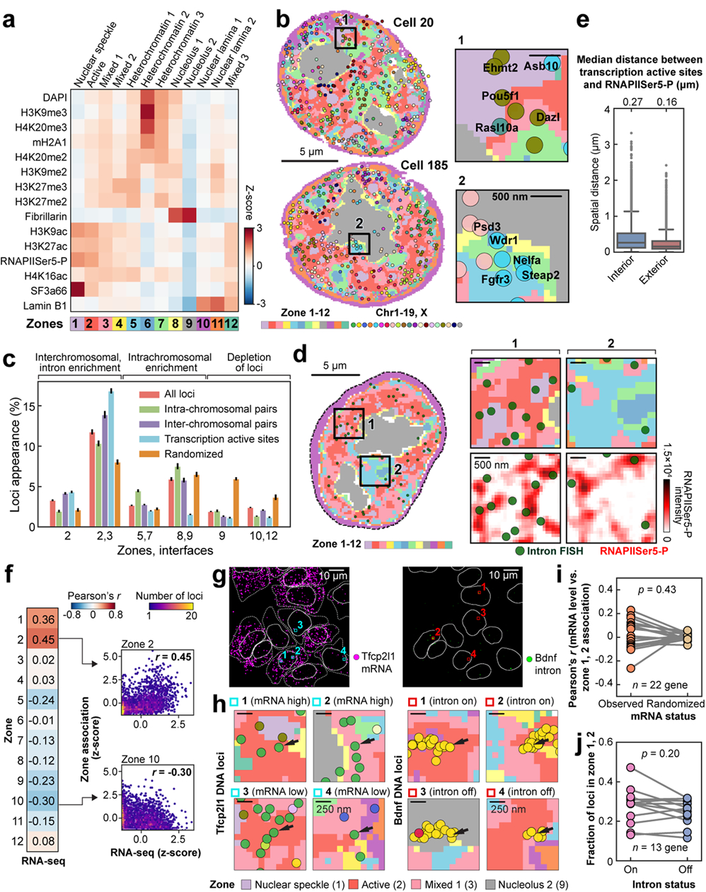
a, Heatmap for differential enrichment of individual chromatin markers in each zone. b, Reconstructions for nuclear zones and DNA loci at a single z plane. Zoomed-in views (right) show gene loci such as Pou5f1 in zone 1 or interfaces 1/2 (top) and loci around nucleolus and heterochromatin zones (bottom). c, Frequency of DNA loci or transcription active sites (TAS) association with zones/interfaces in single cells. Mean values from 20 bootstrap trials are shown with error bars corresponding to standard errors. d, TAS targeted by 1,000 gene intron FISH and nuclear zones. Zoomed-in views show the enrichment of TAS at the interfaces of nuclear zones (top right panels) and at the exterior of the RNAPIISer5-P staining (background-subtracted, bottom right panels). e, Spatial distance from TAS to RNAPIISer5-P staining interior and exterior voxels. The boxplots represent the median, interquartile ranges, whiskers within 1.5 times the interquartile range, and outliers. f, Pearson correlation of bulk RNA-seq⁴⁹ and zone assignment for all 1 Mb resolution loci (n = 2,460 loci). Right panels show density plots for individual loci. n=201 cells for all DNA loci (a-f) and n=172 cells for TAS (c-e) in two independent experiments. g, Representative maximum intensity z-projected RNA seqFISH images. White lines show segmented nucleus (left and right) and cytoplasm (left). h, Zoomed-in views of g represent the zones around Tfcp2l1 (left) and Bdnf DNA loci (right) with black arrows. Tfcp2l1 is shown with 1 Mb resolution and Bdnf is shown with 25 kb resolution DNA seqFISH+ data. i, Correlation between mRNA counts of the profiled genes and their association to active zones (zone 1, 2) in single cells. Each dot represents a gene (22 genes, n = 125 cells). j, Comparison between intron state and active zone (zone 1, 2) association of the corresponding alleles (13 genes, n = 125 cells). p values were calculated with a two-sided Wilcoxon’s signed-rank sum test, and cells in the center field of views were used in i, j.

For each DNA locus, we assigned a zone or an interface if more than one zone were present (see Methods). Some loci had characteristic zone associations, such as Pou5f1 (Oct4) associated with active zone 2 and interfaces 1/2 and 2/3 (Fig. 3b, Extended Data Fig. 8i, j and Supplementary Table 4). Many loci were enriched at interfaces between zones (Fig. 3b, c, Extended Data Fig. 8f, k and Supplementary Table 5), consistent with the observation of loci near the exterior of nuclear bodies and chromatin marks (Fig. 2e, g). For example, DNA loci are 46.3% more likely to be detected at interfaces 2/3 than random chance (Fig. 3c). Furthermore, pairs of interchromosomal loci were enriched at the active interfaces 2/3 while pairs of intrachromosomal loci were enriched at the heterochromatic interfaces 5/7 and nucleolus interfaces 8/9 (Figure 3c). We note that IF images and zone assignments were limited by diffraction and background, and that even finer granularity would be observed with super-resolution imaging of the IF markers (see Methods).

Active loci are pre-positioned

Simultaneous imaging of nascent transcription active sites (TAS) by intronic FISH against 1,000 genes²⁰, 14 IF markers and DAPI in the same cells showed that transcription active sites appear at the surface, rather than the center, of RNAPII dense regions in the nuclei (Fig. 3d, eand Extended Data Fig. 8h). They also appeared in the interfaces between active, and mixed zones (2/3) twice as frequently as compared to by random chance, 16.8% vs 8.0% (Fig. 3c, Extended Data Fig. 8k, Supplementary Table 5). Average expression level across 1 Mb correlated with the association with active and nuclear speckle zones, and interfaces (Fig. 3f, Extended Data Fig. 8l, m), consistent with previous findings³⁷.

However, in single cells, we observed little correlation between mRNA and intron expression and proximity with active and speckle zones amongst the genes we examined (27 genes for mRNA spanning a large range of expression levels and 14 genes for intron) (Fig. 3g–j, Extended Data Fig. 8n, o). Given the typically shorter lifetime of introns and mRNAs (minutes to hours respectively) compared to the possibly longer timescale of chromosomal positioning, it is likely that most genes are not dynamically positioned to the active zones (zone 1, 2) for transcription. Rather, it is likely that most genes are pre-positioned to those zones/interfaces, and their positioning may be determined by underlying epigenetic states as well as other factors such as neighboring gene density⁷.

Global chromatin states are heterogeneous

mESCs have been shown to exist as metastable transcriptional states^40–42 with subpopulations of differential gene expression profiles characterized both by scRNA-seq⁴² and mRNA seqFISH (Extended Data Fig. 9a–c, Supplementary Table 6). We observed that the overall intensities of IF signals in the nucleus also showed substantial heterogeneities among single cells (Fig. 4a). Clustering analysis of the IF data (Fig. 4b and Extended Data Fig. 9d, e) showed at least 7 distinct states based on global chromatin modification levels, with most marker levels independent from cell-cycle phases (Extended Data Fig. 9f). Interestingly, IF states only partially overlapped with the transcriptional states. For example, Zfp42, Nanog and Esrrb expressing “ground” pluripotent state cells as well as Otx2 expressing orthogonal “primed” state cells are present in most IF clusters (Fig. 4b and Extended Data Fig. 9e). In addition, the global levels of H3K27me3 and mH2A1 were associated with naive or ground pluripotent states whereas H3K9me3 was associated with primed pluripotent states (Extended Data Fig. 9g–j). These observations at the single-cell level extend the previous bulk studies^43,44 showing increased total H3K27me3 levels and decreased H3K9me3 heterochromatin clusters in 2i-grown naive mESCs compared to serum-grown mESCs.

Figure 4. Global chromatin states are highly variable and dynamic in single cells.

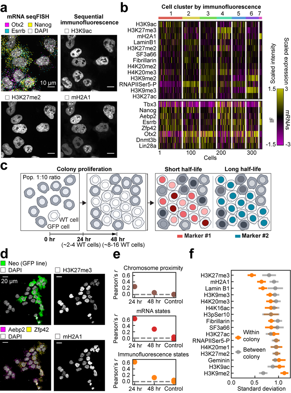
a, The intensities of IF markers show heterogeneities in single cells. Images are from the same z section. Scalebars, 10 μm. b, Heatmap of cell clusters with distinct IF profiles. Bimodally expressed Nanog, Esrrb and Zfp42⁴¹ are distributed over several IF clusters. n = 326 cells in the center field of views from two biological replicates. c, Schematic of colony tracing experiments. Intensity of markers with fast dynamics are expected to be heterogeneous within a colony. d, Representative maximum intensity z-projected images for one 48-hour colony, showing heterogeneities in mRNA (left) and IF markers (right). Scalebars, 20 μm. e, Mean Pearson correlation between cells within colonies decays slowly for mRNA and chromatin states, and quickly for chromosome proximities. Control measures correlation between colonies for both 24- and 48-hour datasets. f, Standard deviation of individual IF marker intensities in 48-hour colonies compared to those between colonies. H3K27me3 and mH2A1 have less variance in cells within a colony, which can be seen in d. Mean values from 20 bootstrap trials are shown with error bars corresponding to standard errors (e, f). n = 117 unlabeled cells within colonies in 48-hour dataset. n=53 cells in 24-hour dataset.

Chromatin states persist across generations

To examine whether the heterogeneity in chromatin states, mRNA expression and chromosome organization are stable or are dynamic over generations, we performed clonal analysis experiments. If clonally related cells have similar molecular states, then those states are likely to have slow dynamics, and vice versa (Fig. 4c). We seeded unlabeled mESCs among GFP-positive mESCs at a 1:10 ratio and cultured them for 24 and 48 hours, which are approximately 2 and 4 generations respectively, such that each unlabeled mESC colony likely arises from a single cell (Fig. 4c, d and Extended Data Fig. 10a).

Overall mRNA and chromatin profiles were highly correlated amongst most cells within a colony at the 24 hr time point (Fig. 4e, Extended Data Fig. 10b), and maintained some correlation even at the 48 hr time point. In contrast, chromosome proximities are preserved across one cell cycle between sisters but are then rapidly lost after 2 generations (Fig. 4e, Extended Data Fig. 10c–e), consistent with previous studies with targeted chromosomes or regions^45–48. Interestingly, the dynamics of individual IF markers such as mH2A1 and H3K27me3, were highly correlated within colonies but not between colonies, suggesting that these chromatin features are heritable across at least 3–4 generations (Fig. 4f). On the other hand, many IF marks, such as H3K9ac, did not correlate within a colony nor between colonies, suggesting that these features are rapidly fluctuating.

Discussion

Our spatial multimodal approach with DNA seqFISH+ along with multiplexed IF and RNA seqFISH enables profiling of chromosome structures, nuclear bodies, chromatin states, and gene expression within the same single cells. The precisely aligned images over multiple modalities allowed us to observe invariant features across nuclei despite the heterogeneity in chromosome structures in single cells. Interestingly, many DNA loci, especially active gene loci, reside at the surface of nuclear bodies and zone interfaces. Functionally, if target loci reside on surfaces, do regulatory factors diffuse in 2D or 3D to search for their target genes? Lastly, the observation of heterogeneous and long-lived global chromatin states raises the question of whether these states have distinct pluripotency and differentiation potentials and could represent “hidden variables” in differentiation experiments, which warrants further investigation. We anticipate that the spatial multi-omics approaches will enable further exploration of those questions in many biological contexts.

Methods

Data reporting.

No statistical methods were used to predetermine sample size. The experiments were not randomized and the investigators were not blinded to allocation during experiments and outcome assessment.

DNA seqFISH+ encoding strategy.

A 16-base coding scheme with 5 rounds of barcoding is used in DNA seqFISH+ for the 1 Mb resolution data in fluorescent channel 1 (643-nm) and 2 (561-nm) (Extended Data Fig. 1b, Supplementary Table 2). The first 3 rounds of barcoding codes for 16^3=4,096 unique barcodes. Two additional rounds of parity check (linear combinations of the first three rounds) are included. 2,048 barcodes are selected to correct for dropouts in any 2 out of 5 rounds of barcoding and used in both channel 1 and 2. The 16-pseudocolor base is generated by hybridizing the sample with 16 different readout oligos sequentially.

To image 20 distinct regions (1.5–2.4 Mb in size) with 25 kb resolution, a combined strategy of diffraction limited spot imaging and chromosome painting is used in channel 3 (488-nm) (Extended Data Fig. 1c, Supplementary Table 2), by extending previously demonstrated “track first and identify later” approach¹⁹. For the initial 60 rounds, 25 kb regions are readout one at a time on all 20 chromosomes in each round of hybridization. These 60 rounds can resolve the 25 kb loci within each distinct region but cannot distinguish which chromosome the loci belong to. The next 20 rounds are used to resolve the identities of the 20 distinct regions or chromosomes by painting the entire region (1.5–2.4 Mb) one at one time. With this strategy, identities for 1,200 loci are decoded.

To implement these strategies, 80 unique readouts are used in each fluorescent channel for a total of 240 readouts for 3 channels.

Primary probe design.

RNA seqFISH probes were designed as described previously^20,21. In brief, 35-nt RNA target binding sequences, 15-nt unique readout probe binding sites for each RNA target, and a pair of 20-nt primer binding sites at 5’ and 3’ end of the probe for probe generation (see ‘primary probe synthesis’) are concatenated. Marker genes (Supplementary Table 6) were selected based on previous single cell imaging and RNA-seq studies in mESCs^20,41,42,49.

For DNA seqFISH+ target region selection (Supplementary Table 1), the unmasked and repeat-masked GRCm38/mm10 mouse genome FASTA files were downloaded from Ensembl release 93⁵⁰. To select target regions for channel 1, the entire mouse genome was split into candidate target regions of 25 kb. Masking coverage was evaluated for each region using the repeat-masked genome. Regions with a high percentage of masked bases were removed from consideration. Then target regions were further selected to space out approximately 2 Mb in the genome coordinates. To select target regions for channel 2, candidate genes related to mESCs pluripotency and differentiation were selected from previous studies^35,42,51, and then 25 kb regions were selected by centering the transcription starting sites of the genes. To select target regions for channel 3, gene loci with various expression levels in mESCs as well as gene poor regions were initially selected as a 2.5 Mb block, and splitted into 25 kb blocks. Only a single 2.5 Mb region was selected per chromosome.

Region-specific primary probes were designed as previously described for single-stranded RNA²¹ with some modifications. The target region was extracted from the unmasked genome. Probe sequences were produced by taking the reverse complement of 35-nt sections of the target region. Starting from the 5’ end of the forward strand, candidate probes were tested for viability, shifting one base at a time. Probes that contained five or more consecutive bases of the same kind, or had a GC content outside of 45–65%, were considered non-viable. Each time a viable probe was discovered, evaluation was switched to the opposite strand, starting 19-nt downstream from the start of the viable probe to mitigate cross-hybridization between neighboring probes. This procedure was repeated until the end of the target region was reached.

Next, the probes were aligned to the unmasked mouse genome for off-target evaluation using Bowtie2⁵². Any alignment containing at least 19 matched bases that fell outside the genomic coordinates of the target region was considered off-target. Probes with more than 10 total off-target hits were dropped. Off-target hits were grouped into 100 kb bins and stored for use in the final probe selection. Bins were overlapped by 50 kb so that closely grouped hits could not evade the filter by splitting into two bins. Additionally, probes were checked for matches with a BLAST⁵³ database constructed from common repeating sequences in mammals. The FASTA file for “Simple Repeat” sequences for “Mammalia only” was downloaded from Repbase⁵⁴. All probes with at least 19 matched bases with the repeats index were dropped. After filtering the probes, all remaining probes were evaluated for potential cross-hybridization using BLAST⁵³. Any probe pairs with at least 19 matched bases were dropped in the final probe selection.

Final probe sets were selected to maintain probe specificity, and to achieve a relatively uniform spacing of probes on the target sequence. Final probes were selected one by one, starting with the target region with the fewest remaining probes. The probe that minimized the sum of the squares of distances between adjacent selected probes and the start and end coordinates of the target region was selected. After selecting a probe, any probes that were found to cross-hybridize with at least 19-nt to the selected probe were dropped. As probes were added, their off-target hits were summed by bin. If the addition of a probe resulted in any bin having 10 total hits, all remaining unselected probes that had an off-target hit in that bin were dropped. For channel 1 and 2 probes, once 200 probes were selected for a target region, all remaining probes for that region were dropped. These two channels labeled 2,460 loci spaced approximately 1 Mb apart (1.04 ± 0.78 Mb as mean ± standard deviation) across the whole genome. For the channel 3 probes, regions containing up to 150 probes were kept and other regions were dropped, and as a result, 1.5–2.4 Mb of 20 distinct regions containing 60 of 25 kb regions were finally selected as the 1,200 loci.

Primary probes were then assembled similar to previous seqFISH studies^18–21,55. At each locus targeted, we used up to 200 primary probes within the 25 kb genomic region as described above to image individual loci as diffraction limited spots based on DNA FISH^56–59 and Oligopaint¹⁶ technologies. For Mb resolution DNA seqFISH+ in channel 1 and 2, primary probes consist of the genomic region specific 35-nt sequences, flanked by the five unique 15-nt readout probe binding sequences, which correspond to pseudo-channel in each barcoding round, and a pair of 20-nt primer binding sites at the 5’ and 3’ end of the probe. For 25 kb resolution DNA seqFISH+ in channel 3, primary probes consist of the genomic region specific 35-nt sequences, flanked by three identical binding sites of a 15-nt readout probe, which corresponds to one of the 60 sequential rounds for the diffraction limited spot imaging, and two identical binding sites for a 15-nt readout probe, which corresponds to one of the 20 distinct regions for the chromosome painting, and 20-nt primer binding sites at the 5’ and 3’ end of the probes.

Primary probe synthesis.

Primary probes were generated from oligoarray pools (Twist Bioscience) as previously described^18–21,55 with some modifications. In brief, probe sequences were amplified from the oligo pools with limited two-step PCR cycles (first step PCR primers, 4-fwd: 5’-ATGCGCTGCAACTGAGACCG; 4-rev: 5’-CTCGACCAAGGCTGGCACAA; second step PCR primers, 4-fwd: 5’-ATGCGCTGCAACTGAGACCG; 4-T7rev: 5’-TAATACGACTCACTATAGCTCGACCAAGGCTGGCACAA), and PCR products were purified using QIAquick PCR Purification Kit (Qiagen 28104). Then in vitro transcription (NEB E2040S) followed by reverse transcription (Thermo Fisher EP0751) were performed. For the DNA seqFISH+ primary probes, the forward primer (4-fwd) with 5’ phosphorylation was used at the reverse transcription step to allow ligation of the primary probes as described below (see ‘Cell culture experiment’). After reverse transcription, the single-stranded DNA (ssDNA) probes were alkaline hydrolysed with 1 M NaOH at 65°C for 15 min to degrade the RNA templates, and then neutralized with 1 M acetic acid. Then, probes were ethanol precipitated, and eluted in nuclease-free water.

For the repetitive element DNA FISH probes, LINE1 and SINEB1 probes were similarly generated except using mouse genomic DNA template extracted from E14 mESCs with DNeasy Blood & Tissue Kits (Qiagen 69504) for PCR, followed by in vitro transcription and reverse transcription steps. Primers for LINE1 and SINEB1³³ contain readout probe binding sites as overhangs to allow readout probe hybridization and stripping with seqFISH routines. Genome targeting sequences of the primary probes were 113-nt and 117-nt for LINE1 and SINEB1, respectively. In contrast, the centromeric minor satellite DNA (MinSat) and telomere probes were generated as dye-conjugated 15-nt probes in the same way as readout probes (see ‘Readout probe design and synthesis’) using the following sequences (MinSat: 5’-CACTGTTCTACAATG; telomere: 5’-AACCCTAACCCTAAC), which directly target genomic DNA.

Readout probe design and synthesis.

Readout probes of 12–15-nt in length were designed for seqFISH as previously described^20,21. In brief, a set of probe sequences was randomly generated with combinations of A, T, G or C nucleotides with a GC-content range of 40–60%. To minimize cross-hybridization between the readout probes, any probes with ten or more contiguously matching sequences between the readout probes were removed. The readout probes for sequential immunofluorescence were similarly designed except ‘C’ nucleotide is omitted⁶⁰. The 5’ amine-modified DNA oligonucleotides (Integrated DNA Technologies) with the readout probe sequences were conjugated in-house to Alexa Fluor 647-NHS ester (Invitrogen A20006) or Cy3B-NHS ester (GE Healthcare PA63101) or Alexa Fluor 488-NHS (Invitrogen A20000) as described before^20,21, or fluorophore conjugated DNA oligonucleotides were purchased from Integrated DNA Technologies. In total, 240 unique readout probes²¹ were designed and synthesized for DNA seqFISH+ experiments, and subsets of those readout probes were used for RNA seqFISH experiments. The cost for 240 readout probes for DNA seqFISH+ were approximately $15,000 with 5’ amine-modified DNA oligonucleotides and dye conjugation in-house, and $50,000 with fully labeled purchase, which can be used over hundreds or thousands of experiments.

DNA-antibody conjugation.

Preparation of oligo DNA conjugated primary antibodies was performed as described before³¹ with modifications. In brief, to crosslink thiol-modified oligonucleotides to lysine residues on antibodies, BSA-free antibodies were purchased from commercial vendors whenever possible. Antibodies (90–100 μg) were buffer-exchanged to 1× PBS using 7K MWCO Zeba Spin Desalting Columns (Thermo Scientific 89882), and reacted with 10 equivalent of PEGylated SMCC cross-linker (SM(PEG)2) (Thermo Scientific 22102) diluted in anhydrous DMF (Vector Laboratories S4001005). The solution was incubated at 4°C for 3 hours, and then purified using 7K MWCO Zeba Spin Desalting Columns. In parallel, 300 μM 5’ thiol-modified 18-nt DNA oligonucleotides (IDT) were reduced by 50 mM dithiothreitol in 1× PBS at room temperature for 2 hours, and purified using NAP5 columns (GE Healthcare 17-0853-01). Then maleimide activated antibodies were mixed with 6–15 equivalent of the reduced form of the thiol-modified DNA oligonucleotides in 1× PBS at 4°C overnight. DNA-primary antibody conjugates were washed with 1× PBS four times and concentrated using 50 KDa Amicon Ultra Centrifugal Filters (Millipore, UFC505096). The concentration of conjugated oligo DNA and antibody with BCA Protein Assay Kit (Thermo Scientific 23225) were quantified using Nanodrop.

For the BSA containing primary antibodies, SiteClick R-PE Antibody Labeling Kit (Life Technologies S10467) was used to conjugate the antibodies with 10–20 equivalent of 5’ DBCO-modified 18-nt DNA oligonucleotides (IDT). The oligo conjugated antibodies were validated by SDS-PAGE gel and immunofluorescence, and stored in 1x PBS at −80°C as small aliquots.

Cell culture and preparation.

E14 mESCs (E14Tg2a.4) from Mutant Mouse Regional Resource Centers were maintained under serum/LIF condition as previously described^20,41. A stable E14 line that targets endogenous repetitive regions with the CRISPR/Cas system⁶¹ was generated similarly to the previous study¹⁹. In brief, PiggyBac vectors, PGK-NLS-dCas9-NLS-3xEGFP, carrying a separate puromycin resistance cassette under an EF1 promoter, and mU6-sg3632454L22Rik(F+E), carrying a separate neomycin resistance cassette under a SV40 promoter, were constructed. A single-guide RNA (sgRNA) sequence (5’-GGAAGCCAGCTGT) was used to target repetitive regions at the 3632454L22Rik gene locus in X chromosome. To create the stable E14 line (GFP/Neo E14) with those vectors, transfection was performed with FuGENE HD Transfection Reagent (Promega E2311), and cells were selected with puromycin (Gibco A1113803) at 1 μg/mL. After the selection, single clones were isolated manually, and stable labeling of the locus was verified by imaging. The cell lines were authenticated by DNA seqFISH+ (Extended Data Fig. 3a–g), multiplexed immunofluorescence (Extended Data Fig. 6a–f), and RNA seqFISH (Extended Data Fig. 9a–c), all of which gave results consistent with the embryonic stem cell identity. The cells were not tested for mycoplasma contamination.

E14 cells were plated on poly-D-lysine (Sigma P6407) and human laminin (BioLamina LN511) coated coverslips (25 mm × 60 mm)²⁰, and incubated for 24 or 48 hours. Then cells were fixed with freshly made 4% formaldehyde (Thermo Scientific 28908) in 1× PBS (Invitrogen AM9624) at room temperature for 10 minutes. The fixed cells were washed with 1× PBS a few times, and stored in 70% ethanol at −20°C¹². In the case of co-culture experiments with unlabeled E14 cells and the GFP/Neo E14 cells (monoclonal line), cell densities were counted and cell lines were mixed with a 1:10 ratio.

Cell culture experiment.

The fixed and stored cell samples were dried, and permeabilized with 0.5% Triton-X (Sigma-Aldrich 93443) in 1× PBS at room temperature for 15 minutes after attaching a sterilized silicon plate (McMASTER-CARR 86915K16) with a punched hole to the coverslip to use it as a chamber. The samples were washed three times with 1× PBS and blocked at room temperature for 15 minutes with blocking solution consisted of 1× PBS, 10 mg/mL UltraPure BSA (Invitrogen AM2616), 0.3% Triton-X, 0.1% dextran sulfate (Sigma D4911) and 0.5 mg/mL sheared Salmon Sperm DNA (Invitrogen AM9680). Then DNA oligo-conjugated primary antibodies listed below were incubated in the blocking solution with 100-fold diluted SUPERase In RNase Inhibitor (Invitrogen AM2694) at 4°C overnight. The typical final concentration of DNA conjugated primary antibodies used were estimated as 1–5 ng/μL. The samples were washed with 1× PBS three times and incubated at room temperature for 15 minutes, before post-fixing with freshly made 4% formaldehyde in 1× PBS at room temperature for 5 minutes. Next, the samples were washed with 1× PBS six times and incubated at room temperature for 15 minutes. The samples were then further post-fixed with 1.5 mM BS(PEG)5 (PEGylated bis(sulfosuccinimidyl)suberate) (Thermo Scientific A35396) in 1× PBS at room temperature for 20 minutes, followed by quenching with 100 mM Tris-HCl pH7.4 (Alfa Aesar J62848) at room temperature for 5 minutes. After the post-fixation, the samples were washed with 1xPBS and air dried after removing the custom silicon chamber.

The oligo DNA conjugated primary antibodies used were as follows: mH2A1 (Abcam ab232602), E-Cadherin (R&D AF748), Fibrillarin (C13C3) (Cell Signaling 2639BF), Geminin (Abcam ab238988), GFP (Invitrogen G10362), H3 (Active Motif 39763), H3K27ac (Active Motif 39133), H3K27me2 (Cell Signaling 9728BF), H3K27me3 (Cell Signaling 9733BF), H3K4me1 (Cell Signaling 5326S), H3K4me2 (Cell Signaling 9725BF), H3K4me3 (Active Motif 39915), H3K9ac (Active Motif 91103), H3K9me2 (Abcam ab1220), H3K9me3 (Diagenode MAb-146–050), H3pSer10 (Millipore 05–806), H4K16ac (EMD Millipore 07–329), H4K20me1 (Abcam ab9051), H4K20me2 (Abcam ab9052), H4K20me3 (Active Motif 39671), Lamin B1 (Abcam ab220797), RNAPII Ser5-P (Abcam ab5408), SF3a66 (Abcam ab77800). Two antibodies (E-Cadherin and GFP) were only included in the clonal tracing experiments. Several antibodies (H3, H3K4me1, H3K4me2 and H3K4me3) were excluded from the downstream analysis due to the quality of antibody staining with oligo-conjugation.

After the immunofluorescence preparation above, custom-made flow cells (fluidic volume ~30 μl), which were made from glass slide (25 × 75 mm) with 1 mm thickness and 1 mm diameter holes and a PET film coated on both sides with an acrylic adhesive with total thickness 0.25 mm (Grace Bio-Labs RD481902), were attached to the coverslips. The samples were rinsed with 2× SSC, and RNA seqFISH primary probe pools (1–10 nM per probe) and 10 nM polyT LNA oligo with a readout probe binding DNA sequence (Qiagen) were hybridized in 50% hybridization buffer consisted of 50% formamide (Invitrogen AM9342), 2× SSC and 10% (w/v) dextran sulfate (Millipore 3710-OP). The hybridization was performed at 37°C for 24–72 hours in a humid chamber. After hybridization, the samples were washed with a 55% wash buffer consisting of 55% formamide, 2× SSC and 0.1% Triton X-100 at room temperature for 30 minutes, followed by three rinses with 4× SSC. Then samples were imaged for RNA seqFISH as described below (see ‘seqFISH imaging’). Note that immunofluorescence signals were imaged at this step for validation in Extended Data Fig. 2f, g.

After RNA seqFISH imaging, the samples were processed for DNA seqFISH+ primary probe hybridization. The samples were rinsed with 1× PBS, and incubated with 100-fold diluted RNase A/T1 Mix (Thermo Fisher EN0551) in 1× PBS at 37°C for 1 hour. Then samples were rinsed three times with 1× PBS, followed by three rinses with a 50% denaturation buffer consisting of 50% formamide and 2× SSC and incubation at room temperature for 15 minutes. Then the samples were heated on the heat block at 90°C for 4.5 minutes in the 50% denaturation buffer, by sealing the inlet and outlet of the custom chamber with aluminum sealing tapes (Thermo Scientific 232698). After heating, the samples were rinsed with 2× SSC, and DNA seqFISH+ primary hybridization buffer consisting of ~1 nM per probe, ~1 μM LINE1 probe, ~1 μM SINEB1 probe, 100 nM 3632454L22Rik fiducial marker probe (IDT), 40% formamide, 2× SSC and 10% (w/v) dextran sulfate (Millipore 3710-OP) was hybridized at 37°C for 48–96 hours in a humid chamber. After hybridization, the samples were washed with a 40% wash buffer consisting of 40% formamide, 2× SSC and 0.1% Triton X-100 at room temperature for 15 minutes, followed by three rinses with 4× SSC.

Then samples were further processed to “padlock”^62,63 primary probes to prevent the loss of signals during 80 rounds of DNA seqFISH+ imaging routines (see ‘seqFISH imaging’). A global ligation bridge oligo (IDT) was hybridized in a 20% hybridization buffer consisting of 20% formamide, dextran sulfate (Sigma D4911) and 4xSSC at 37°C for 2 hours. The 31-nt global ligation bridge (5’-TCAGTTGCAGCGCATGCTCGACCAAGGCTGG) was designed to hybridize to 15-nt of the DNA seqFISH+ primary probes at 5’ end and 16-nt at the 3’ end. Then, samples were washed with 10% WB for three times and incubated at room temperature for 5 minutes. After three rinses with 1× PBS, the samples were then incubated with 20-fold diluted Quick Ligase in 1× Quick Ligase Reaction Buffer from Quick Ligation Kit (NEB M2200) supplemented with additional 1 mM ATP (NEB P0756) at room temperature for 1 hour to allow ligation reaction between 5’- and 3’-end of the DNA seqFISH+ primary probes. We note that unlike the conventional padlock primary probe design^62,63, our primary probe ligation sites were on the 31-nt global ligation bridge at the primer binding sites (Extended Data Fig. 1a, b), and not on the genomic DNA. Then the samples were washed with a 12.5% wash buffer consisting of 12.5% formamide, 2× SSC and 0.1% Triton X-100, followed by three rinses with 1× PBS.

The samples were then processed for amine modification and post-fixation to further stabilize the primary probes. The samples were rinsed with 1× Labeling Buffer A, followed by incubation with 10-fold diluted Label IT Amine Modifying Reagent in 1× Labeling Buffer A from Label IT Nucleic Acid Modifying Reagent (Mirus Bio MIR 3900) at room temperature for 45 minutes. After three rinses with 1× PBS, the samples were fixed with 1.5 mM BS(PEG)5 in 1× PBS at room temperature for 30 minutes, followed by quenching with 100 mM Tris-HCl pH7.4 at room temperature for 5 minutes. The samples were washed with a 55% wash buffer at room temperature for 5 minutes, and rinsed with 4× SSC for three times. Then samples were imaged for DNA seqFISH+ and sequential immunofluorescence as described below (see ‘seqFISH imaging’).

The 1,000 gene intron experiments in Fig. 3c–e and Extended Data Fig. 8h, k were performed similarly with minor modifications. E14 coverslips were prepared and processed by following the sequential immunofluorescence steps above. After the sequential immunofluorescence preparation, 1,000 gene intron FISH probes²⁰ were hybridized in the 50% hybridization buffer at 37°C for 24 hours in a humid chamber. Then samples were washed with the 55% wash buffer at 37°C for 30 minutes, followed by three rinses with 4× SSC. Then samples were imaged for intron FISH and sequential immunofluorescence as described below (see ‘seqFISH imaging’).

The telomere validation experiments in Extended Data Fig. 2a, b were performed similarly with minor modifications. Samples were prepared as described above and hybridized with a telomere primary probe, consisting of 20-nt telomere targeting sequence, five 15-nt readout probe binding sites and 20-nt primer binding sites with 5’ phosphorylation, in the 20% hybridization buffer at 37°C overnight in a humidity chamber. Then samples were prepared with or without ligation and post-fixation steps as described above. After samples were imaged with the imaging procedure (see ‘seqFISH imaging’), samples were incubated in the 55% WB at 37°C for 16 hours. Then the original positions were imaged again under the same imaging procedure (see ‘seqFISH imaging’) to evaluate the “padlocking” efficiency across different conditions.

Microscope setup.

All imaging experiments were performed with the imaging platform and fluidics delivery system similar to those previously described^20,21. The microscope (Leica DMi8) was equipped with a confocal scanner unit (Yokogawa CSU-W1), a sCMOS camera (Andor Zyla 4.2 Plus), 63× oil objective lens (Leica 1.40 NA), and a motorized stage (ASI MS2000). Fiber coupled lasers (643, 561, 488 and 405 nm) from CNI and Shanghai Dream Lasers Technology and filter sets from Semrock were used. The custom-made automated sampler was used to move designated readout probes in hybridization buffer from a 2.0 mL 96-well plate through a multichannel fluidic valve (IDEX Health & Science EZ1213-820-4) to the custom-made flow cell using a syringe pump (Hamilton Company 63133–01). Other buffers were also moved through the multichannel fluidic valve to the custom-made flow cell using the syringe pump. The integration of imaging and the automated fluidics delivery system was controlled by custom written scripts in μManager⁶⁴.

seqFISH imaging.

The sequential hybridization and imaging routines were performed similarly to those previously described^20,21 with some modifications. In brief, the sample with the custom-made flow cell was first connected to the automated fluidics system on the motorized stage on the microscope. Then the regions of interest (ROIs) were registered using nuclei signals stained with 5 μg/mL DAPI (Sigma D8417) in 4× SSC. RNA seqFISH imaging was performed with the sequential hybridization and imaging routines described below first. After the completion of RNA seqFISH imaging, the samples were disconnected from the microscope, and proceeded to the DNA seqFISH+ procedures (see ‘Cell culture experiment’). For the DNA seqFISH+ and sequential IF imaging, the registered ROIs for RNA seqFISH were loaded and manually corrected to ensure to image the same ROIs as RNA seqFISH imaging, and following routines were performed.

All the sequential hybridization and imaging routines below were performed at room temperature. The serial hybridization buffer contained two or three unique readout probes (10–50 nM) with different fluorophores (Alexa Fluor 647, Cy3B or Alexa Fluor 488) in 10% EC buffer (10% ethylene carbonate (Sigma E26258), 10% dextran sulfate (Sigma D4911) and 4× SSC), and was picked up from a 96-well plate and flow into the flow cell for 20 minutes incubation. For DNA seqFISH+ experiments, readout probes (Alexa Fluor 647, Cy3B or Alexa Fluor 488) for sequences designated as fiducial markers were also included in the serial hybridization buffer to allow image registration at the subpixel resolution. After the serial hybridization, the samples were washed with 1 mL of 4× SSCT (4× SSC and 0.1% Triton-X), followed by a wash with 330 uL of the 12.5% wash buffer. Then, the samples were rinsed with ~200 μl of 4× SSC, and stained with ~200 uL of the DAPI solution for 30 seconds. Next, anti-bleaching buffer was flown through the sample for imaging. The anti-bleaching buffer was made of 50 mM Tris-HCl pH 8.0 (Invitrogen 15568025), 300 mM NaCl (Invitrogen AM9759), 2× SSC, 3 mM trolox (Sigma 238813), 0.8% D-glucose (Sigma G7528), 1,000-fold diluted catalase (Sigma C3155), 0.5 mg/mL glucose oxidase (Sigma G2133)²⁰ for E14 experiments, and made of 50 mM Tris-HCl pH 8.0, 4× SSC, 3 mM trolox, 10% D-glucose, 100-fold diluted catalase, 1 mg/mL glucose oxidase (Sigma G2133)²¹ for unlabeled E14 and GFP/Neo E14 line clonal experiments.

Snapshots were acquired with 0.25 μm z-steps over 6 μm z-slices with 643-nm, 561-nm, 488-nm and 405-nm fluorescent channels per field of view, except for RNA seqFISH in the clonal experiments acquired with 0.75 μm z-steps with 643-nm, 561-nm, 488-nm fluorescent channels. After image acquisition, 1 mL of the 55% wash buffer was flown for 1 minutes to strip off readout probes, followed by an incubation for 1 minutes before rinsing with 4× SSC. The serial hybridization, imaging and signal extinguishing steps were repeated until the completion of all rounds. During the RNA seqFISH and DNA seqFISH+ imaging routines, blank images containing only autofluorescence of the cells were imaged at the beginning and end of the routines. During the DNA seqFISH+ imaging, images containing only fiducial markers were also imaged at the beginning and at the end of the routines for the image alignment (see ‘Image Analysis’). Images were manually checked at the end of all imaging routines and in case problematic hybridization rounds such as off-focus appeared, those hybridization rounds were repeated.

The each readout probe hybridization and stripping routine took approximately 30 minutes. Imaging time per position took around 2.5–6 minutes at each hybridization round with our microscope setup and imaging conditions described above, and we typically imaged for 30 minutes per hybridization round with 5–10 positions. In total, it took approximately 80 hours to complete the 80 rounds of the hybridization and imaging routine for the DNA seqFISH+ experiments.

Image Analysis.

To correct for the non-uniform background, a flat field correction was applied by dividing the normalized background illumination with each of the fluorescence images while preserving the intensity profile of the fluorescent points. The background signal was then subtracted using the ImageJ rolling ball background subtraction algorithm with a radius of 3 pixels.

FISH spot locations were obtained by using a laplacian of gaussians filter, semi-manual thresholding as described below, and a 3D local maxima finder. Subsequently the locations were super resolved using a 3D radial center algorithm^65,66. Briefly, a 3×3×3 cube of pixels around a local maxima found above the specified threshold was taken from the aligned and background subtracted image. This sub-image was then used to calculate the sub-pixel location of the RNA molecule or DNA locus and the mean standard deviation (average of the standard deviation in each dimension) of the intensity cloud using a 3D radial center algorithm. A MATLAB implementation of the algorithm can be found on the Parthasarathy lab website. The resulting RNA or DNA spot locations were further filtered based on the size of the sigma values.

To find the optimal threshold values for the spot detection, threshold values for RNA seqFISH were updated manually. In contrast, for DNA seqFISH+, 29 incremental threshold values, were initially applied to the images in the first position. The number of spots and median spot intensity in the nuclei were computed for each of the 29 thresholds across 80 hybridizations. Then the threshold value for the first hybridization round was manually chosen, and threshold for the other hybridizations were selected such that the number of dots detected matches most closely to those expected from the codebook. For example, if hyb 1 targets 30 loci and hyb 2 targets 60 loci, then hyb 2 should have twice as many dots as hyb 1. In this process, we assumed all loci can be detected with the same detection efficiency on average. In addition, the median intensities from the adjacent threshold values were compared, and whenever intensity differences are more than 15%, a more stringent threshold value was taken to fulfill this criteria to minimize non-specific spot detection. These processes were performed in individual fluorescent channels independently. Similarly, we corrected the threshold values across positions by computing the ratio of the median intensities relative to those from the first position per hybridization in order to minimize detection bias across different positions.

To align spots or images in different channels to those in the reference channel (643-nm), chromatic aberration shifts were corrected using the fiducial markers to calculate the offsets. To align RNA seqFISH and sequential immunofluorescence images in different hybridization rounds, reference channels (either DAPI or polyA staining) were aligned using 2D phase correlations along every axis iteratively to find a consensus transformation for alignment as described before²⁰. The 2D phase correlation algorithm is implemented in MATLAB with the function imregcorr. To align DNA seqFISH+ spots in different hybridization rounds, fiducial markers were identified in each image by searching for the known ‘constellation’ seen in images containing only the fiducial markers. To identify a first pair of distant fiducial markers, the vector describing the relative position of the known markers was compared with those separating similarly oriented pairs of FISH spots in each image. Most, if not all, of the fiducial marker ‘constellation’ can then be recovered by searching for each fiducial marker at its known location relative to that of previously identified fiducial markers in the image. Further alignment to correct any rotation between RNA and DNA FISH images was done as follows. First, both image stacks to be aligned (DAPI or immuno- staining) were converted to 2D images using a maximum intensity projection in the z-dimension. The resulting 2D images were aligned using a one plus one evolutionary optimization method to maximize the Mattes Mutual Information between the images with the transformation constrained to only rigid transforms with a maximum of 500 iterations. This algorithm is implemented in MATLAB with the function imregtform. Once 2D alignment with both translation and rotation was obtained, one stack was transformed using the found transformation. The image stacks were then projected along the x axis and aligned using a normalized cross-correlation to determine the first estimate of the z-dimension offset. The image was then projected along the y axis to find a second estimate of the z-dimension offset using the same method. The two offsets were averaged.

To assign mRNA spots to individual cells, the processed spots were collected within individual cytoplasmic ROIs, which were segmented manually from polyA or E-Cadherin images. Similarly, to assign intron and DNA spots to individual cells, the spots within individual nuclear ROIs from DAPI images²⁰ were collected. By comparing the centroids between cytoplasmic ROIs and nuclear ROIs, numbers from both ROIs were matched. Only cells at the center of the fields of view were preserved for the RNA analysis to avoid biasing the RNA distribution.

For channel 1 and 2 barcode decoding in DNA seqFISH+, once all potential points in all hybridizations were obtained, points were matched to potential barcode partners in all other barcoding rounds of all other hybridizations using a 1.73 (square root of 3) pixel search radius to find symmetric nearest neighbors in 3D. This process was performed in each nuclear ROIs. Point combinations that constructed only a single barcode were immediately matched to the on-target barcode set. 2 rounds of error corrections were implemented out of 5 total barcoding rounds. For points that matched to multiple barcodes, the point sets were filtered by calculating the residual spatial distance of each potential barcode point set and only the point sets giving the minimum residuals were used to match to a barcode. If multiple barcodes were still possible, the point was matched to its closest on-target barcode with a hamming distance of 1. If multiple on target barcodes were still possible, then the point was dropped from the analysis as an ambiguous barcode. This procedure was repeated using each barcoding round as a seed for barcode finding and only barcodes that were called similarly in at least 4 out of 5 seeds were used in the analysis. This criteria on average dropped 19.8 ± 2.8% (mean ± standard deviation) of identified barcode spots compared to the less stringent criteria using at least 3 out of 5 seeds, while minimizing the detection of false positive barcode dots. The false negatives can be caused by this dropout of barcode dots as well as by incomplete denaturation of chromosomal DNA or hybridization of primary probes. For the false positive estimates, both blank barcodes and on-target barcodes were run simultaneously. Those blank barcodes consisted of all the remaining barcodes out of 2,048 barcodes that allow 2 rounds of error corrections in 5 total barcoding rounds.

For channel 3 decoding in DNA seqFISH+, once all potential points in the first 60 hybridizations (hyb 1–60) were obtained, intensities of all the potential chromosome paint partners in the other 20 hybridizations (hyb 61–80) were computed on the rounded pixels where points were found. At this step, each point has 20 intensity values, corresponding to those from individual chromosome paints. Those chromosome paint intensities found on the points in nuclei from all positions and all hybridization rounds (hyb 1–60) were grouped by chromosome, and then z score was calculated. The z score values were thresholded with 1, and each point was assigned with unique chromosome identity, whose value was above the threshold. Only a minimum fraction of points (<3%) were assigned to multiple chromosomes and dropped as ambiguous points. In addition, points without any chromosome assignment were dropped as ambiguous points.

Exterior and Interior voxels of IF markers

For the sequential immunofluorescence image processing, in contrast to spot detection processing as described above, background subtraction was not applied to the images, except for marker edge detection described below and RNAP II Ser5-P visualization shown in Fig. 3d and Extended Data Fig. 8h. The alignment and correction for chromatic aberration shifts between different fluorescent channels were performed as described above. Then intensity values for all the voxels within individual nuclear ROIs were obtained for all IF channels as well as repetitive elements (telomere, MinSat, LINE1 and SINEB1) and DAPI. The edge detection for chromatin marker exterior quantification was performed using Find Edges function in Image J with background subtracted images (rolling ball radius 3 pixels), and then the intensity values were obtained in the same way as the aligned images above.

After image processing steps above, pixel information was converted to physical distance based on the microscope setup and imaging condition with 103 nm for x and y pixel and 250 nm for z pixel for the subsequent downstream analysis.

Analysis of sequencing-based data.

Hi-C data from NCBI GEO (accession GSE96107) was processed using Juicer tools⁶⁷ and contact maps containing Knight-Ruiz normalized counts⁶⁸ were obtained. SPRITE data were obtained from the 4D Nucleome data portal (data.4dnucleome.org, accession 4DNESOJRTZZR). ChIP-seq data for H3K27me3, H3K9ac, H3K27ac were obtained from ENCODE (encodeproject.org, accession ENCSR000CFN, ENCSR000CGP, ENCSR000CGQ) as bigWig tracks and the average relative signal in each genomic bin was calculated using the UCSC Genome Browser program bigWigAverageOverBed. DamID data were obtained from NCBI GEO (accession GSE17051) and the genomic coordinates of DamID microarray probes were converted from mm9 to mm10 using the UCSC Genome Browser program liftover. DamID values were calculated as the mean DamID score within each genomic bin. Repli-seq data were obtained from NCBI GEO (accession GSE102076) and the replication timing at each genomic bin was calculated as the log2 ratio of early and late S fractions. GRO-seq data were obtained from NCBI GEO (GSE48895) and aligned to mm10 using Bowtie2⁵² to create bam files. Read counts at each genomic bin were obtained from bam files using bedtools multicov. Hi-C data was binned at the 25, 50, 100, 250, 500 kb and 1 Mb resolution, and all the other data were binned at the 1 Mb resolution. For Hi-C analysis, overlapping regions within a given bin size were excluded from the analysis (Fig. 1f with 100 kb bin resolution, Fig. 1g with 25 kb bin resolution, and Extended Data Fig. 3 with described bin resolution).

Visualization of seqFISH data.

DNA seqFISH+ data were visualized using PyMOL (Molecular Graphics System, Version 2.0 Schrödinger, LLC.) by generating a .xyz file containing the x,y,z coordinates of each FISH probe coordinate. Each coordinate was displayed as a sphere, and sticks were drawn between coordinates that were consecutive in the genome. Immunofluorescence and repetitive element DNA FISH signals were visualized by displaying a surface around x,y,z coordinates with intensity Z-score values above 2.

Estimation for DNA seqFISH+ detection efficiency.

We estimated the detection efficiency of DNA seqFISH+ considering the cell cycle distribution as described before¹⁹. Briefly, typical cell cycle phases distribute as 20% in G1, 50% in S and 30% in G2/M phase in mESCs. Given the number of DNA loci is 2 in G1, 3 in S and 4 in G2/M phase, the average number of spots expected per each locus is 3.1 in a single cell, which can be half for chromosome X (n = 180 loci in DNA seqFISH+) in male diploid E14 cells. In our DNA seqFISH+ experiments, we observed 5,616.5 ± 1,551.4 (median ± standard deviation) for 3,660 loci in single cells, and the detection efficiency can be estimated as 50.7 ± 14.0% (median ± standard deviation).

DNA proximity map analysis.

To generate a pairwise proximity map from the DNA seqFISH+ dataset, for each locus in a single cell, the identities of other loci within a search radius of 500 nm for channel 1 and 2 and 150 nm for channel 3 were tabulated. The total occurrence of any pairwise interaction was normalized by the product of the occurrence frequency of each of the loci. The proximity map was compared with the Hi-C map²³ in Fig. 1g. The proximity maps for all chromosomes for both 1 Mb and 25 kb data are shown in Extended Data Fig. 3 and 4.

Physical distance vs genomic distance.

In each cell, two homologous chromosomes were separated by finding the consensus between two clustering algorithms: Spectral method in the FindClusters function in Mathematica and Ward method. For most chromosomes in single cells, the two copies of homologous chromosomes occupied distinct regions in the nucleus, while in some cells, they were fused together. In a small percentage of cells, 3 or more alleles of the same chromosome could be observed. However, in a vast majority of cells, only 2 chromosomal territories were observed indicating that replicated chromosomes mostly stay together⁶⁹ until segregation. For the 25 kb data, the alleles were separated by the DBSCAN clustering algorithm in scikit-learn library in python.

Along each allele of a given chromosome in single cells, we calculated the physical distances between all pairs of detected loci and paired them with their genomic distances. For a fixed genomic distance, the median physical separation values are shown in Fig. 1h for the 1 Mb data for all the chromosomes, and Fig. 1i for the 25 kb resolution data.

IF normalization and clustering analysis.

For the voxel-based multiplexed IF analysis, we first aligned the sequential immunofluorescence data across all rounds of hybridization (see ‘Image Analysis’). Then voxels in each channel were binned 2×2×1 (200 nm × 200 nm × 250 nm), because the diffraction limit is approximately 200–250 nm in the fluorescence channels imaged. All subsequent data analyses were performed on the binned data. Because tens of millions of voxels from all of the cells were too numerous for clustering analysis, representative subsets of voxels were selected, clustered and used as a training set to train a model which then propagated the cluster identification to all voxels in the data. To do so, voxels from a single Z plane (plane 13, approximately midpoint in the cell) out of 25 z-slices for all cells were selected. In each cell, individual channels were z-score normalized. The voxels with total z-score values more than 0 summed over 16 IF channels were selected and normalized by the total z-score to account for voxel to voxel intensity variations. All pixels of the cells within the first experiment (n = 201 cells) were then combined and one out of every 200 pixels are selected and clustered by hierarchical clustering using the Mathematica Agglomerate function and Ward distance option. 10 clusters or nuclear zones were assigned to all 60,482 pixels as the training set. These classified zone definitions were then propagated to the rest of the pixels in each cell normalized by the above procedure using the GradientBoostedTree option in the Classify function in Mathematica. Separately, pixels with Lamin B1 and Fibrillarin marker z-score >1 were assigned to the nuclear lamina and nucleolus zones. The 44,000 pixels, which are assigned to one of the 12 nuclear zones and contain 16 intensity values from individual IF markers, were then visualized in Extended Data Fig. 8b with Uniform Manifold Approximation and Projection (UMAP)⁷⁰ using a umap-learn library in python.

To compare the IF zone assignments with and without DNA FISH, we use the IF data from the intron experiments. We used the same training set from the DNA seqFISH+ dataset and propagated the classifiers to the IF data in the intron experiment. We found similar composition of zones in the intron experiments, indicating that IF data are not affected significantly with the denaturing conditions in DNA FISH. Results are shown in Extended Data Fig. 8d.

Similarly, we downsampled the number of IF marks used to assign the zones. We reduced the number of IF marks systematically and used 80% of the pixels as the new training set to determine what fraction of the pixels are assigned correctly. Results are shown in Extended Data Fig. 8e. 20 random subsets of IF marks are drawn for each downsample IF number. Band shows the standard deviation of the correct zone assignment.

We note that the zone assignments are based on the combinatorial chromatin marks at each diffraction limited pixel. So the resolution and the boundary of the zones are also diffraction limited, which could contribute to some of the mixed zones detected. For example, we cautiously note that previous super-resolution imaging⁷¹ showed that Lamin B1 meshwork is around 100 nm thick at the nuclear periphery, while our zone analysis showed Lamin B1 enriched zone 11 and mixed zone 12 were typically found at the pixels further than 100 nm from the nuclear periphery (Fig. 3b, Extended Data Fig. 8f–h), possibly due to the limitation of the resolution. In addition, we note that background signals of the multiplexed IF could also affect the nuclear zone distribution patterns. Future works with super-resolution microscopy may resolve the mixed regions at finer resolution.

DNA loci to IF marker interactions.

We calculated the spatial distances between each DNA locus and the nearest “hot” IF voxel, defined by two standard deviations above the mean value for each IF marker. We also calculated the distance of each DNA loci to the exterior of IF nuclear bodies, also two standard deviations above the mean for the edge processed image described under ‘Image Analysis’ (Extended Data Fig. 5b) for each IF marker. Both metrics, defined as interior and exterior distances, are highly correlated (Extended Data Fig. 5e, f). From this distance metric, we generated a “chromatin profile” by counting the percentage of cells in which each DNA loci is within 300 nm of the surface of an IF mark, the resolution of the diffraction-limited immunofluorescence images. These chromatin profiles were correlated with ChIP-seq²⁴, DamID³⁵, and SPRITE⁷ datasets (Extended Data Fig. 6a, b).

For Lamin B1, we calculated the distances from DNA loci to Lamin B1 signals with two and three standard deviations away from the mean intensity, as well as using only Lamin B1 signals at the nuclear periphery (as determined from the convex hull of the nuclear pixels) and the nuclear periphery pixels. Similar Lamin B1 or nuclear periphery association profiles were observed for all analysis in correlation plots (Extended Data Fig. 6c) across DNA loci (Extended Data Fig. 6e).

Fixed loci were determined as loci that appear 2 standard deviations above the mean percentage score for each IF mark. The distance between fixed loci and the exterior and interior of nuclear bodies, pixels 2 standard deviation above the mean in the edge processed and raw images for each IF mark, are shown in Fig. 2e. The average expression level for fixed loci associated with different IF marks are calculated from bulk RNAseq and shown in Extended Data Fig. 8m.

Chromosome configuration (Supplementary table 3) of the fixed points calculates the fraction of cells (n = 446 cells) for each chromosome that contains at least one fixed loci from a given pair of the IF markers. This metric measures how likely fixed points from different IF markers span nuclear bodies in single cells.

Previous literature reported the approximate locations of ribosomal DNA repeat sequences (rDNA) on a subset of chromosomes with non-sequencing methods. In mouse, rDNA arrays are encoded on the centromere-proximal regions of chromosomes 12, 15, 16, 18 and 19, and the patterns of distribution differ in a mouse strain-specific manner^72–74. We found all fixed loci for the nucleolar marker, Fibrillarin in those chromosomes (n = 39, 1, 22, 30 and 41 loci for chromosome 12, 15, 16, 18 and 19) with less enrichment on chromosome 15 (Fig. 2d, h). Importantly, previous studies using the allele of the 129 mouse strain reported the loss of rDNA or nucleolar enrichments on chromosome 15^7,73,74, consistent with our observation with E14 cells derived from 129/Ola mouse strain.

The chromatin profiles for all loci were clustered by hierarchical clustering using the Agglomerate function in Mathematica with the Ward distance option and plotted in tSNE (Extended Data Fig. 7a) with scikit-learn library in python. 15 chromatin marks along with DAPI were used, and 4 clusters were selected. Cluster 1 is enriched in repressive markers such as H3K9me3, mH2A1 and DAPI. Cluster 2 was enriched in interactions with Fibrillarin and associated with nucleolus. Cluster 3 was enriched in active marks such as RNAPII Ser5-P, H3k27ac and SF3a66 (speckle marker). Cluster 4 was enriched in Lamin B1. In individual cells, loci associated with each cluster were mapped onto the chromosome structure images shown in Extended Data Fig. 7b. To calculate the spatial proximity spatial proximity of loci within and between clusters, we computed the frequency of finding a loci from a given cluster within a 1 μm radius with another loci of the same or different cluster identity. The total number of intra-cluster and inter-cluster interactions were tabulated and normalized to unity. Randomized data was generated by scrambling the cluster identities of individual loci in cells while keeping the total number of loci within each cluster the same within that cell. The proximity frequency for observed and randomized data for each cell are shown as boxplots in Extended Data Fig. 7d and for different search radii in Extended Data Fig. 7e. Similar analysis is performed for A/B compartment assignments²³, and shown in Extended Data Fig. 7f–j. The loci without A/B compartment assignments in the study were excluded from the analysis.

Association of loci with zones.

For each DNA loci decoded from the DNA seqFISH+ experiment, the nearest pixels within 300 nm and the zone assignments for those pixels were collected in each cell. It is possible to have a locus be in association with multiple zones. If a locus interacts with more than two zones, for example Pou5f1 (Oct4) in cell 38 is interacting with zone 1, 2, and 8, then its zone interactions were divided into pairs of zones, or “interfaces”. In other words, that locus was counted 1/3 toward each of the interfaces (1, 2), (2, 8), and (1, 8). For individual loci, the frequencies of appearing in all zones and interfaces were normalized to unity and shown in Extended Data Fig. 8i, j. For the analysis shown in Fig. 3c and Extended Data Fig. 8k, the total number of DNA loci detected each zone and interfaces are tabulated and normalized to unity for each zone or interfaces between pairs of zones. The same analysis for zone proximity was performed on the set of loci that are interacting with other loci on the same chromosomes (intrachromosomal) and with loci on the other chromosomes (interchromosomal) within 300 nm. Similarly, the introns from the 1,000 gene experiments were tabulated for their zone and interface assignments. Randomized DNA loci were generated by selecting a random set of voxels in the nucleus while keeping the total number of DNA loci the same in a given cell. Then the voxels were offset by a random xyz value with a 100 nm radius. To bootstrap all of the data sets, we randomly sampled 150 cells out of n = 201 cells with 20 trials and calculated the mean and standard errors.

Correlation of zone with gene expression.

To calculate the correlation between expression and zone assignment, we took each channel 1 and 2 locus and computed the total RNAseq FPKM values⁴⁹ within 50 kb upstream and downstream of that locus. We normalized the total frequency of appearing in one of the zones or interfaces to unity for each loci. We then correlated the Log (1+expression value) of all 2,460 regions with the frequency of finding them in each of the zones/interfaces. Similar analysis was performed for GRO-seq⁷⁵ using Log (1+GRO-seq value) and Replication timing⁷⁶ datasets with mESCs.

To determine whether we can predict the mean expression values for each locus based on its zone association profiles, we estimated the expression level for a given loci as a sum of the product between the normalized frequency of being in each zone/interface for that loci and the Pearson correlation coefficient between the zone/interface with the mean expression value across all the loci. The estimated expression values for all 2,460 loci were correlated with the actual expression values with a Pearson’s coefficient of 0.54.

For calculating the correlation between mRNA expression levels with zone assignments in single cells, we first z-scored the single cell mRNA seqFISH measurements for 22 genes after normalizing by Eef2 expression levels to account for cell size differences and selecting cells in the center field of view (n = 125 in replicate 1). The genes with mean copy numbers of > 10 per cell were used. Lack of correlation was observed with both biological replicates, but only the cells in replicate 1 were shown to eliminate potential contributions from batch to batch variations. We counted the frequency of each of the measured loci within 300 nm of a voxel with an active or speckle zone assignment (zone 1 and 2), normalized by the total number of voxels that were within 300 nm of the DNA locus. The Pearson coefficient was computed between the z-scored expression value and the active/speckle zone association frequency. To randomize the sample, we shuffled the z-score normalized expression values with active/speckle zone occupancy from different cells over 20 randomized trials. The correlation coefficient for each gene was calculated and plotted in Fig. 3i and Extended Data Fig. 8n.

For calculating the correlation between intron expression levels with zone assignments in single cells, we classified the corresponding DNA loci as “ON” or “OFF” based on whether introns were bursting at that loci or not for 13 introns measured. The genes with mean burst frequencies of > 0.1 per cell were used. Then the active and speckle zone occupancy for loci in each category was calculated and shown in Fig. 3j and Extended Data Fig. 8o with each point representing one intron.

Colony analysis.

For cells within the unlabeled E14 colonies, we compute the correlation of the IF states, RNA states and chromosome structures between pairs of cells. Individual RNA levels were normalized by Eef2 expression level and then z-scored across all cells in the experiment. The chromosome proximity correlations between cells are computed as follows. First, a 20×20 chromosome to chromosome proximity matrix is generated for each cell with a search radius of 2.5 μm. Then the correlations between cells were computed as the Pearson correlation coefficient of the entries of the two matrices. The intensity of individual IF marks was first normalized by the total intensity of all IF marks and then z-scored within each field of view. The averages of the cell pair correlation values for IF, RNA and chromosomes are shown in Fig. 4e for 24 hour and 48 hour clonal tracing as well as controls (correlation of pairs of cells between colonies in the 24 hour and 48 hour data). In addition, we computed the variance of individual IF marks within single colonies in the 48 hour experiment compared to the variance between cells of different colonies. IF marks that have longer time scale correlation showed lower variance within colonies compared to the variance between colonies in Fig. 4f.

Normalization of global chromatin levels in single cells.

To remove the contributions from cell size, background signals, the affinity of antibody used, as well as differences between biological replicates, we constructed a generalized linear model (GLM) for the sequential immunofluorescence data using the glm() function in R, which had been used to adjust for systematic bias in single cell RNA sequencing data^77–79, for each chromatin mark i, using a Gaussian error distribution:

$$log{Y}_i~{\beta }_0+\sum _j{\beta }_j{X}_j$$

Y_i represents the vector of total fluorescence intensity of chromatin mark i across all cells, and X_j is a vector of latent variables contributing to the systematic bias in global chromatin states quantification. We included cell size, total fluorescence intensity over all chromatin marks per cell, experimental replicate ID and field of view (FOV) ID as latent variables in the GLM, and used the Pearson residuals of each fitting as the corrected standardized values of single cell chromatin state.

Characterizing the heterogeneity of global chromatin states in single cells.

We next described the global chromatin heterogeneity between single cells using the adjusted total fluorescence intensities derived from above. Our single cell global chromatin data has less profiled features, and without the sparsity commonly seen in many of the single cell RNA-seq datasets, we were able to directly calculate pairwise similarity of single cells from the adjusted data matrix. A K-nearest neighbor (KNN) graph was computed from the cell-cell Euclidean distance with K = 10 without the four cell cycle markers (Geminin, H4K20me1, H3pSer10 and H4K16ac). The KNN graph was used as the input for Uniform Manifold Approximation and Projection (UMAP)⁷⁰ for two-dimensional visualization (Extended Data Fig. 9d), and was also subsequently transformed into a shared nearest neighbor (SNN) graph for Leiden clustering⁸⁰, with the resolution parameter set to 0.8. The Seurat⁸¹ function FindNeighbors() and FindClusters() were used.

We have then included four markers of cell cycle processes in the analysis: Geminin, H4K20me1, H3pSer10 and H4K16ac^20,82. We constructed a principal curve⁸³ which worked as a non-linear summary of multi-dimensional data, using the function principal_curve() from the R package princurve. Using the projected values onto the principal curve as ordered cell cycle states, we found that H4K20me1 and H4K16ac displayed opposite continuum across single cells (Extended Data Fig. 9f), suggesting that the principal curve depicted a progression from G2/M to S phase.

Characterizing transcriptional heterogeneity of single cells.

Similar to global chromatin states quantification, we constructed a GLM for individual gene expression vector in RNA data, with cell size, total profiled transcripts per cell, experimental replicate ID and FOV ID as latent variables. Pearson residuals were taken as the corrected and standardized expression values.

Given that the majority of mRNA species in this dataset are pluripotency and differentiation genes (e.g. Nanog, Pou5f1, Dnmt3a), we were interested in whether cells could be ordered pseudo-temporally in transcriptional states. We used a diffusion map^84,85 to infer a low-dimensional manifold of RNA seqFISH data with the package destiny⁸⁶, and the first diffusion component in rank was taken as a measurement of pseudotime. All the profiled genes were used to construct pseudotime, except for Cx3cr1, Npy, S100b and Zfp352 (maximum transcript count less than 10 in a cell). To visualize the continuum transcriptional and global chromatin data with respect to pseudotime progression, for every transcript and chromatin mark, we performed a local polynomial regression fitting with span = 0.75 and degree = 2 and generated the fitted values (Extended Data Fig. 9h).

Mapping RNA seqFISH data to single cell RNA sequencing results.

To evaluate whether transcriptional states of mESCs from seqFISH were comparable to those measured by single cell RNA-seq, we constructed a support vector machine (svm) model for mapping seqFISH data to existing scRNA-seq results. Specifically, scRNA-seq data⁴² was downloaded from ArrayExpress, and we retrieved quantifications for cells cultured in serum/LIF condition for analysis. The top 2,000 most variable genes were identified based on dispersion, based on which we ran a principal component analysis (PCA) and used the top 30 components as input for Leiden clustering⁸⁰, with the resolution parameter set to 0.8 in the Seurat⁸¹ function FindClusters(). For data alignment between mESCs quantified by the two technologies, we performed canonical correlation analysis (CCA) to project the two datasets onto a shared space, followed by L2 normalization, using genes detected by both scRNA-seq and seqFISH (40 mRNA markers in total). The aligned data was for svm training and prediction, where the classifier was trained on cells captured by scRNA-seq with 10-fold cross validation, and cluster labels were subsequently transferred to aligned seqFISH data. For joint visualization, we performed UMAP on the L2-normalized CCA embeddings for all cells (Extended Data Fig. 9b).

Statistics and Reproducibility

Cells shown in Figure 1b–d, Figure 2a, and Figure 4a, Extended Data Figure 4a, and 5a,b are representative of the 446 cells imaged in 2 biological replicates. Cells shown in Figure 3 are representative of 201 cells and 172 cells in two independent experiments. Cells shown in Figure 4d and Extended Data Figure 10a are representative of n=117 cells in the 48hr dataset.

Network analysis.

To investigate the relationship of gene and chromatin markers, we first calculated the pairwise Pearson correlation coefficient (PCC) of different genes and chromatin markers using scaled mRNA/antibody by cell matrix (Extended Data Fig. 9e). Then, the results were represented as a network, where a pair of gene-gene, chromatin mark-chromain mark or gene-chromatin mark were connected if the PCC is greater than 0.4. The network was visualized by Cytoscape⁸⁷, and the width of edges in network were weighted by 100^|PCC| to highlight the edges with high correlation (Extended Data Fig. 9i).

Reporting summary.

Further information on research design is available in the Nature Research Reporting Summary linked to this paper.

Extended Data

Extended Data Fig. 1 |. Detailed schematics of the integrated spatial genomics approach with DNA seqFISH+, RNA and intron seqFISH and multiplexed immunofluorescence.

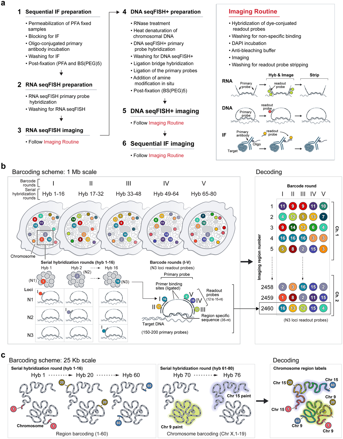
a, Flow chart of the experimental procedures. Samples are fixed with PFA, followed by oligo-conjugated primary antibody incubation, post-fixation with PFA and BS(PEG)5, and RNA seqFISH. Then samples are prepared for DNA seqFISH+. This optimized protocol ensures good alignment between DNA seqFISH+ data with RNA seqFISH and the multiplexed IF data on a voxel by voxel level (see Extended Data Fig. 2). Bottom right cartoon shows imaging routine for RNA FISH and DNA seqFISH+ with primary probes and sequential immunofluorescence with oligo conjugated primary antibodies. b, Schematics of DNA seqFISH+ for the 1 Mb resolution dataset. 5 round of barcoding allows 2,048 barcodes to be detected with 2 rounds of dropout error correction in each fluorescent channel. Two fluorescent channels are used to cover a total of 2,460 loci, spaced approximately 1 Mb apart in the genome. In each round of barcoding, 16 rounds of hybridization are performed to generate 16 pseudocolors. DNA dots detected in each pseudocolor channel are fitted in 3D to determine their super-resolved centroid location and compiled across all 16 pseudocolors to generate a super-resolved localization image. With 5 rounds of barcoding (overall 80 rounds of serial hybridizations), the identity of all DNA loci are decoded. Every DNA loci should appear once in every barcoding round in a single pseudocolor. The barcoding table (Supplementary Table 2) is shown on the right. DNA seqFISH+ probes contain all 5 rounds of barcode readout sequences. Each sequence, for a given barcoding round, has a possible choice of 16 sequences, corresponding to one of the pseudocolors. For each gene, 5 out of the 80 hybridizations will result in hybridization events and fluorescent readout probes bound on the primary DNA hybridizing probes. To preserve the DNA primary probe on the chromosome over all 80 rounds of hybridizations, the primary probes are padlocked^62,63 onto the chromosomes by T4 DNA ligase at the primer binding sites after the initial hybridization (see Methods). c, Barcode scheme for the 25 kb resolution DNA seqFISH+. 60 adjacent 25 kb regions are sequentially readout and imaged in 60 rounds of hybridization. This is carried out in parallel on 20 chromosomes. In other words, each round of hybridization images 20 different loci on different chromosomes. An additional 20 rounds of hybridization are carried out to label each chromosome one at a time to assign chromosomal identity to each locus imaged during the first 60 rounds individually. The 1 Mb resolution data were collected in the 643-nm (channel 1) and 561-nm (channel 2) channels in b, while the 25 kb resolution data were collected in the 488-nm channel (channel 3) in c.

Extended Data Fig. 2 |. Optimization and validation for DNA seqFISH+.

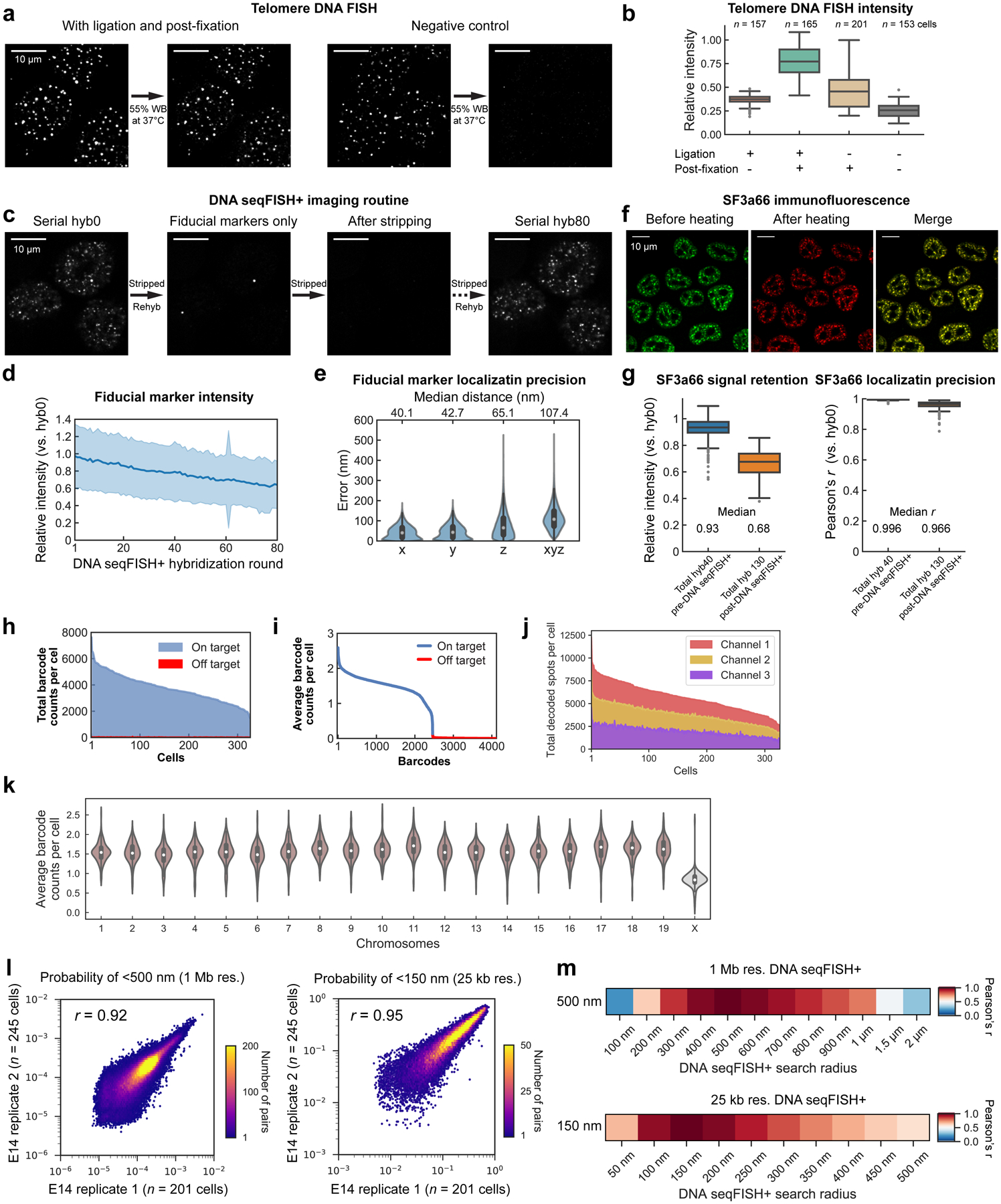
a, Ligation and post-fixation of primary probes prevent their dissociation at the readout probe stripping step, validated by telomere DNA FISH. 55% formamide wash buffer (WB) solution at 37°C was added to the cells for 16 hours with and without the primary probes padlocked^62,63 onto the chromosomal DNA. Probes were retained in the ligated sample, and not retained in the unligated sample. Note that 55% WB was used at room temperature for 2 minutes in each stripping step during the seqFISH routine, which is less stringent than the condition used here. b, Quantification of the signal retention after the harsh wash in a, with telomere DNA FISH across multiple conditions. Total intensities in individual nuclei from a single z section were compared before and after the harsh wash. In the DNA seqFISH+ experiments, the condition with ligation and post-fixation was used. The number of cells from two independent measurements is written in the plot. For the boxplots in b and g, the center line in the boxes marks median, the upper and lower limits of the boxes mark the interquartile range, the whiskers extend to the farthest data points within 1.5 times the interquartile range, and the gray points mark outliers. c, Primary probes are still bound after more than 81 rounds of hybridization, and the specific signals return in the DNA seqFISH+ experiments. Initial hyb0 for DNA seqFISH+ was performed with hyb80 readout probes for comparison. Fiducial markers targeting a repetitive region of the genome with a single primary probe were also imaged initially and included in all 80 imaging rounds for alignment. d, Quantification of the fiducial marker intensities for 80 hybridization rounds in the DNA seqFISH+ experiments, relative to that from hyb0 fiducial markers. Fiducial markers (n = 506–1117 dots per hybridization round) from 446 cells in DNA seqFISH+ experiments were used for quantification. Shaded regions represent the mean (center) with standard deviation (SD). e, Localization errors of fiducial markers across hyb 1 to 80 in the DNA seqFISH+ experiments, n = 71,981 aligned spots for x, y and n = 87,879 aligned spots for z from 446 cells in DNA seqFISH+ experiments. For x and y alignments, we filtered out aligned dots that were more than 2 standard deviations away from the mean displacement at each hybridization, and new alignments were computed. f, Preservation of the nuclear structure through the double fixation procedure. Good colocalization (yellow in the right panel) of the nuclear speckles (SF3a66) before and after heating. g, Quantification of the SF3a66 IF signal retention in the nuclei (left) and localization precision (right) measured by Pearson correlation of pixel intensities in the nuclei with a single z section between hyb0 (pre-DNA seqFISH+ steps) image and hyb40 (pre-DNA seqFISH+ steps) or hyb130 (post-DNA seqFISH+ steps). n = 326 cells in the center field of views from two DNA seqFISH+ biological replicate in g-k. h, Frequencies of on- and off-target barcodes in channel 1 and 2 per cell. On average, 3,636.0 ± 1,052.6 (median ± standard deviation) on-target barcodes and 14.0 ± 7.4 off-target barcodes are detected per cell (n = 326 cells from the center field of views of the two biological replicates). i, Average frequencies of individual on-target and off-target barcodes (n = 4,096 barcodes in channel 1 and 2), demonstrating the accuracy of the DNA seqFISH+. j, The total number of dots detected in each of the fluorescent channels in single cells. Channels 1 and 2 contain the 1 Mb data and channel 3 contains the 25 kb data. k, The average number of dots detected per each locus per cell across all 20 chromosomes. Note that 2 dots per cell are not 100% detection efficiency because some cells are in the G2 phase of the cell cycle (4 alleles in total). X chromosome has half the number of dots detected per locus (0.84 ± 0.21 (median ± standard deviation)) compared to the other autosomes (1.57 ± 0.27), because E14 mESC is a male diploid cell line (see Methods). l, Pearson correlation of probabilities for the pairs of loci within a search radius of 500 nm (1 Mb data) and 150 nm (25 kb data) between two biological replicates of DNA seqFISH+ experiments. All unique intra-chromosomal pairs of loci were calculated for the 1 Mb (n = 2,460 loci) and 25 kb data (n = 1,200 loci) with n = 201, 245 cells in each biological replicate. m, Pearson correlation coefficient of the proximity probability between loci-pairs as a function of search radii in comparison to 500 nm search radius (1 Mb data) and 150 nm search radius (25 kb data) used in l. n = 446 cells from the two DNA seqFISH+ biological replicates.

Extended Data Fig. 3 |. Additional validation for DNA seqFISH+.

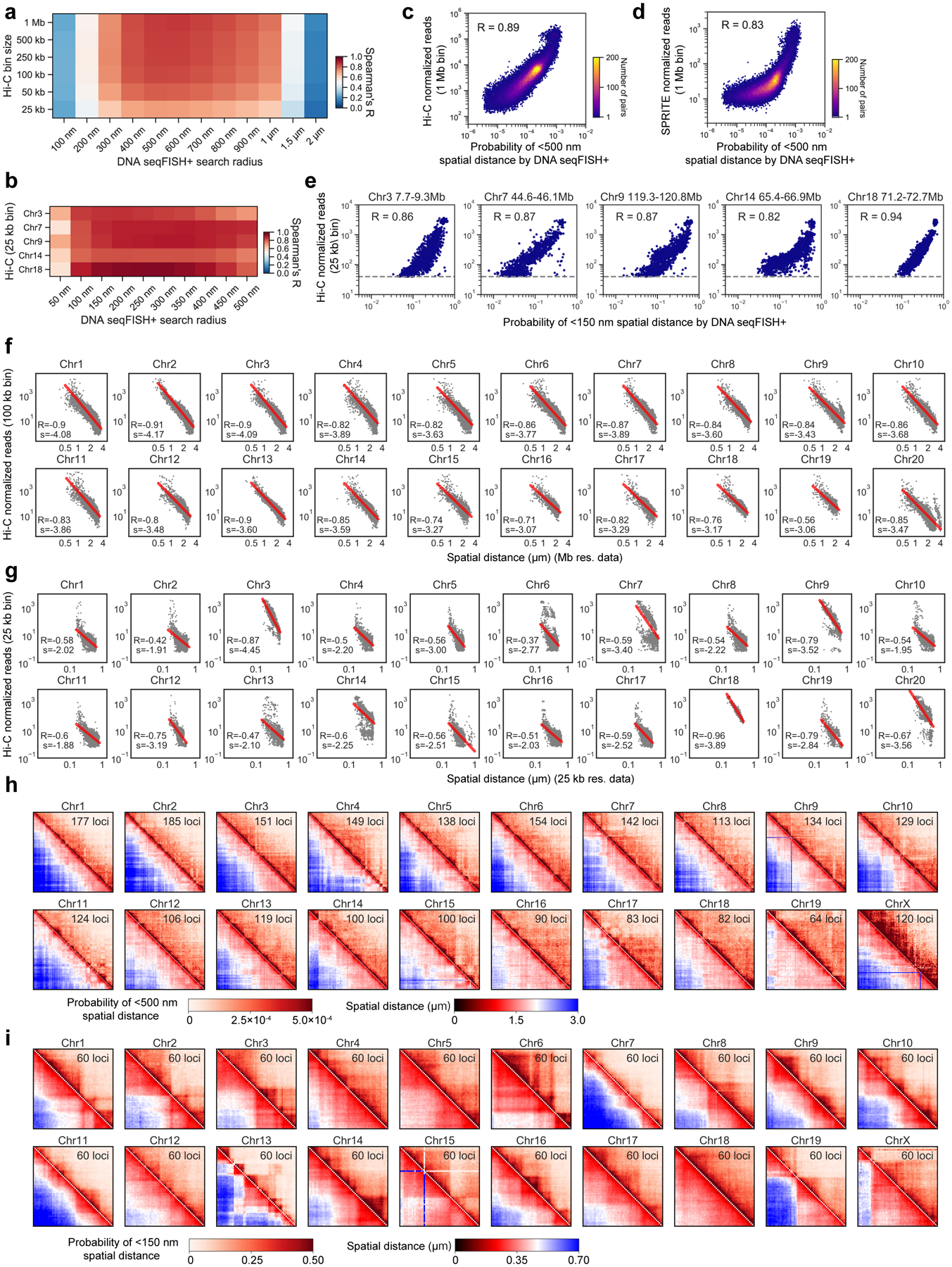
a, b, Spearman correlation between probabilities of pairs of loci within a search radius of 100 nm-2 μm by DNA seqFISH+ and frequencies by Hi-C²³ in mESCs with a certain bin size. All unique intra-chromosomal pairs of loci were calculated for the 1 Mb (n = 2,340 autosomal loci) and 25 kb data (n = 60 loci per chromosome), and overlapping regions within the bin in a were excluded from this analysis. At 1.5 Mb chromosomal regions with 25 kb resolution in b, median Hi-C reads vary depending on the 1.5 Mb regions targeted, ranging from 0.9 to 203.2. We used 5 autosomal regions with Hi-C reads greater than 40 per 25 kb bin for comparison. c, Comparison of probabilities within 500 nm search radius for intra-chromosomal locus pairs in autosomes in DNA seqFISH+ (1 Mb resolution data) and the frequencies in Hi-C²³ data in mESCs. Spearman correlation coefficient of 0.89 computed from n = 84,707 unique intra-chromosomal pairwise combinations. Hi-C data were binned with 1 Mb, and overlapping regions within 1 Mb were excluded from this analysis. d, Comparison of probabilities within 500 nm search radius for the intra-chromosomal locus pairs in autosomes by DNA seqFISH+ (1 Mb resolution data) and frequencies by SPRITE⁷ in mESCs. Spearman correlation coefficient of 0.83. The same binning and filtering were used as the Hi-C analysis in c. e, Comparison of probabilities within 150 nm search radius for the locus pairs in the selected autosomes by DNA seqFISH+ (25 kb resolution data) and frequences by Hi-C²³ in mESCs. Spearman correlation coefficients ranged from 0.82 to 0.94 computed from n = 948–1,776 unique pairwise combinations, using the same selection and filtering criteria as b. f, g, Relationships between median spatial distance of pairs of loci for 1 Mb resolution data in f and 25 kb resolution data in g by DNA seqFISH+ and Hi-C frequencies. The red lines are power-law fits with fitting parameters S shown with Spearman correlation coefficient R. h, i, Heatmaps showing probabilities of pairs of loci within a search radius of 500 nm in h and 150 nm in i (top right triangles), and median spatial distances of pairs of loci (bottom left triangles) in each chromosome for 1 Mb resolution data in h and 25 kb resolution data in i by DNA seqFISH+. n = 446 cells from two biological replicates for DNA seqFISH+ data in a-i.

Extended Data Fig. 4 |. Single cell organization and physical scaling of chromosomes by DNA seqFISH+.

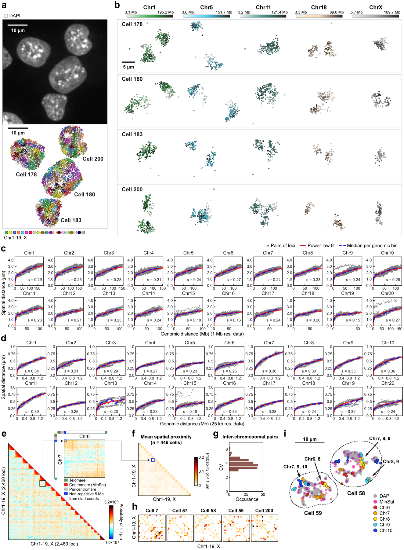
a, DAPI staining image of mESCs (top) and 3D image of corresponding nuclei with individual chromosomes labeled with different colors (bottom). b, 3D image of individual chromosomes, colored based on chromosome coordinates (light to dark colors). Chromosomes are from cells in a. The images are representative of n = 446 cells profiled with DNA seqFISH+. c, d, Scaling of median spatial distance as a function of genomic distance for 20 chromosomes with 1 Mb resolution data in c and 25 kb resolution data in d. Gray dots represent the median distance of the given pairs of loci. Blue dashed lines are the median spatial distance at each genomic distance bin, while red lines are power-law function fits with the fitting parameters in the plots. n = 446 cells. e, The full spatial proximity map between all loci from the 1Mb DNA seqFISH+ data with a search radius of 1 μm (bottom left triangle panel). The zoomed in view of the map for chr6 and chr7 (top right panel), showing the non-repetitive regions near pericentromeric repetitive regions from different chromosomes are more likely to be spatially close to each other. Colorbar is shown in log-scale. f, Mean spatial proximity map for 20 chromosomes, considering only the first 5 Mb non-repetitive regions in each chromosome with a search radius of 1 μm. g, Distribution of CV for spatial proximity from inter-chromosomal pairs in f. h, Single cell version of spatial proximity maps in f show heterogeneity in the spatial proximity between the proximal 5 Mb non-repetitive regions of the chromosomes. i, Single nuclei image shows that proximal 5 Mb non-repetitive regions from only a subset of chromosomes appear near the DAPI-rich pericentromeric heterochromatin regions in individual nuclei. The images are representative of n = 446 cells and the analysis are quantified from 2 biological replicates in e-h.

Extended Data Fig. 5 |. Visualization and validation for sequential immunofluorescence and repetitive element DNA FISH.

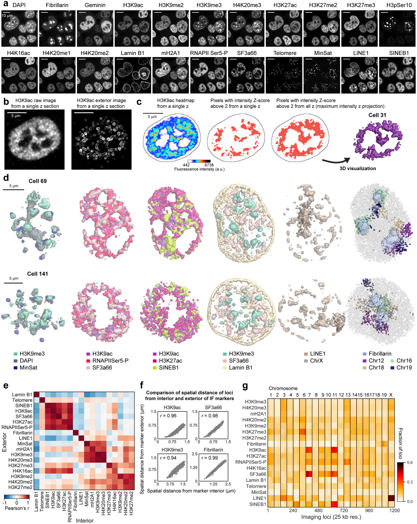
a, 17 antibodies and 4 repetitive elements, including gene-poor long interspersed nuclear elements (LINE1), gene-rich short interspersed nuclear elements (SINEB1), centromeric minor satellite DNA (MinSat), and telomeres, are imaged along with DAPI. Individual cells have different patterns of IF staining. Note the DAPI patterns are not identical between cells. Similarly, marks that are colocalized with DAPI-rich pericentromeric heterochromatin regions are different between cells and even between different pericentromeric regions in a single cell. b, Representative H3K9ac image and edge-transformed image that detects the voxels on the exterior of H3K9ac globules (see Methods). c, Representative H3K9ac images from a single z section or maximum intensity z projection with the intensity Z-score threshold above 2. 3D visualization (right) was performed for the pixels with the intensity Z-score above 2 (see Methods). d, Additional single cell 3D images of IF markers for the pixels with the intensity Z-score above 2. Heterochromatin components (H3K9me3, DAPI, MinSat) were clustered together, while RNAPIISer5-P, active marks (H3K9ac, H3K27ac), SINEB1 and nuclear speckles (SF3a66) were physically proximal. High intensity pixels of LINE1 by DNA FISH localized mainly to the LINE1-rich X chromosome⁸⁸. e, Correlation of chromatin profiles for all 2,460 loci at 1 Mb resolution generated from distance to the interior and exterior voxels of different IF marks (n = 446 cells). f, Scatter plots of the distances from each locus to interior voxels versus exterior voxels that are 2 standard deviations above the mean for 2,460 loci at 1 Mb resolution (n = 446 cells). Pearson correlation coefficients are shown. g, Heatmap showing fraction of loci within 300 nm from IF marks and repetitive elements by DNA seqFISH+ at 25 kb resolution (n = 1,200 loci and 446 cells).

Extended Data Fig. 6 |. Additional visualization and validation for fixed loci and chromatin profiles.

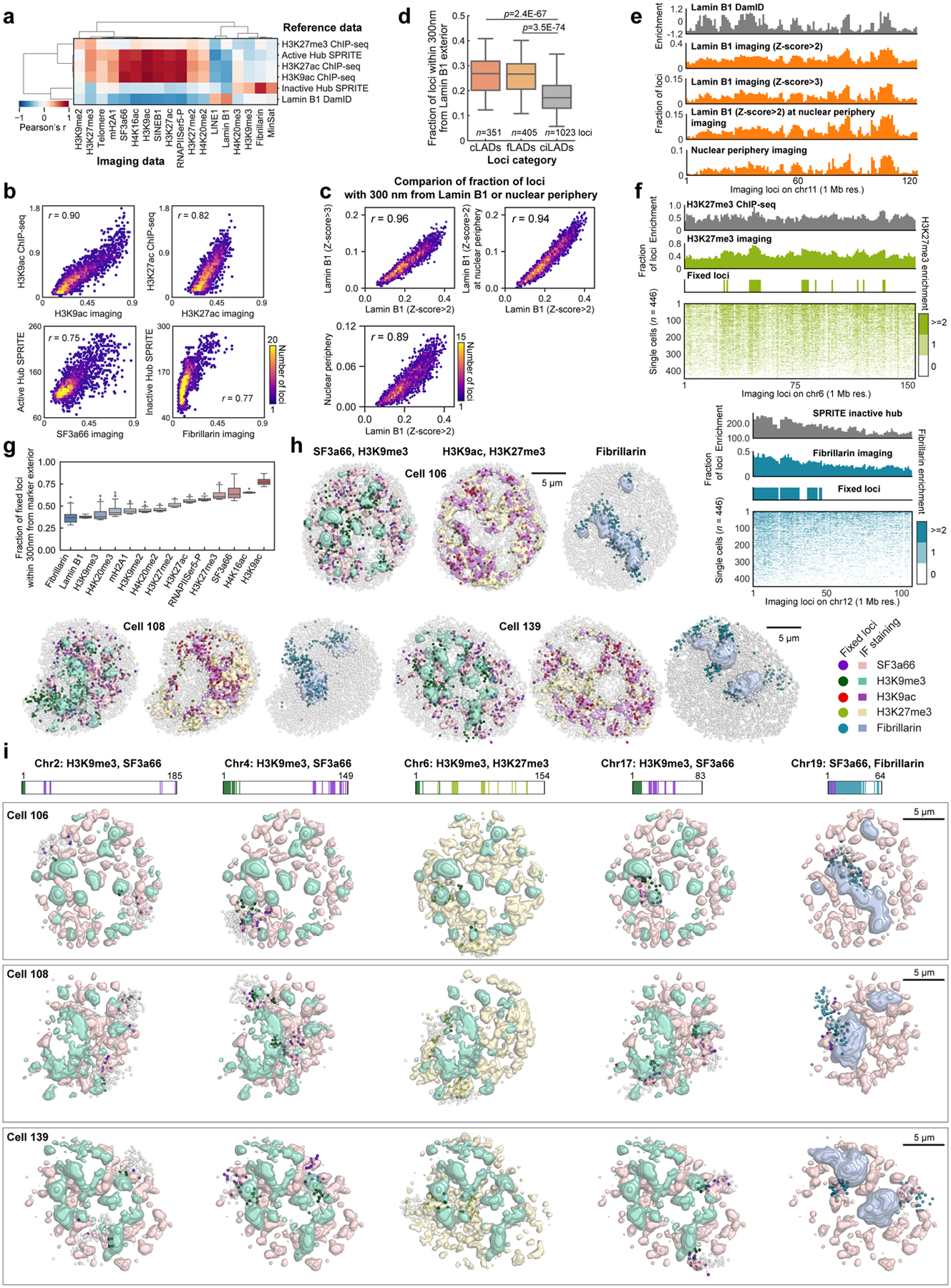
a, Correlation matrix comparing the chromatin profiles by DNA seqFISH+ and IF with other methods^7,24,35. 1 Mb DNA seqFISH+ data were used and the reference data were binned with 1 Mb. Chromatin profiles were computed as the fraction of loci within 300 nm from IF marker exterior for the 2,460 loci (n = 446 cells). b, 2D density plots of individual marker comparison shown in a. n = 2,460 loci. c, Comparison of fraction of loci within 300 nm from Lamin B1 exterior with different thresholding values (Z-score above 2 or 3), or from nuclear periphery computed from convex hull of nuclear pixels (see Methods), showing the good agreement of the profiles in different quantification criteria (n = 2,460 loci from 446 cells). d, Validation of Lamin B1 enrichment with loci categorized as cell-type invariant constitutive lamina-associated domains (cLADs), cell-type dependent facultative LADs (fLADs), and constitutive inter-LADs (ciLADs) assigned from previous DamID studies^35,89. Loci categorized as both cLADs and fLADs show enrichment of proximities to Lamin B1 compared to those from ciLADs, representing a good agreement of our measurement (n = 351, 405, 1,023 loci in each category averaged from 446 cells) with the DamID studies. n is the number of loci. For the boxplots in d and g, the center line in the boxes marks median, the upper and lower limits of the boxes mark the interquartile range, the whiskers extend to the farthest data points within 1.5 times the interquartile range, and the gray points mark outliers. e, Additional visualization for chromatin profiles of Lamin B1 with different criteria in c (n = 446 cells) in comparison with Lamin B1 DamID profile³⁵. To take into account only Lamin B1 staining at the nuclear periphery, we calculated the distances between the DNA loci and the Lamin B1 signal near the convex hull of the nucleus as well as with different intensity thresholds. f, Additional examples for single cell chromatin profiles in comparison with ChIP-seq²⁴ for H3K27me3 (top) and SPRITE⁷. The profiles were computed and are displayed in the same way as Fig. 2c. n = 446 cells. g, The fraction of loci in single cells that are associated with exteriors of IF markers for the fixed loci defined based on the chromatin profiles (n = 446 cells). Note that different IF markers have different thresholds for calling fixed loci. Thus, fixed loci for some IF markers are more consistently associated with the IF marks in single cells. h, Additional 3D images of IF markers and their associated fixed loci. In each cell, 6 IF marks (2 per panel) are shown for visual clarity. i, 5 chromosomes are highlighted in the 3 cells shown in h. The fixed loci for a pair of IF markers are shown for each chromosome in the corresponding image visualization. Fixed loci are shown in colored dots and the remaining loci on the chromosomes are shown as gray dots. The same color codes are used in h.

Extended Data Fig. 7 |. Comparison between population level and single cell level chromosome organization in association with chromatin markers.

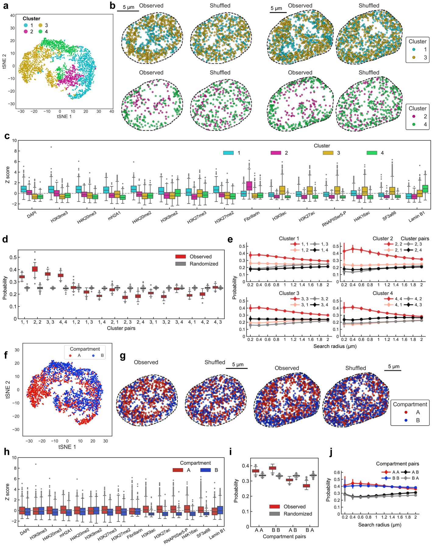
a, Clustering of the ensemble-averaged IF spatial proximity profile of individual loci. n = 2,460 loci (n = 805, 278, 877, 500 loci in each cluster, respectively). b, In individual cells, loci associated with each cluster are mapped onto their spatial location. Note that cluster definitions for DNA loci were obtained from population-averaged data, and those cluster-assigned loci distribution may not necessarily reflect IF marker localization in single cells. c, Boxplot of IF marks for the loci in each of the clusters. Cluster 1 is enriched in repressive markers such as H3K9me3, mH2A1, DAPI. Cluster 2 is enriched in interactions with Fibrillarin. Cluster 3 is enriched in active marks such as RNAPII Ser5-P, H3K27ac and SF3a66 (nuclear speckle marker). Cluster 4 is enriched in Lamin B1. For the boxplots in c, d, h, i, the center line in the boxes marks median, the upper and lower limits of the boxes mark the interquartile range, the whiskers extend to the farthest data points within 1.5 times the interquartile range, and the gray points mark outliers. d, The probability of loci of certain cluster pairs within 1 μm search radius in individual cells. Cluster definitions follow those in a-c. Randomized data were generated by scrambling the cluster identities of individual loci in cells while keeping the total number of loci within each cluster the same within that cell. The probability for observed and randomized data for each cell are shown as boxplots. e, The probability that pairs of loci with cluster assignments are found within a given search radius, as a function of search radius. Error bars represent standard error over 20 bootstrap trials. f, Mapping of the A/B compartment definitions²³ onto the tSNE plot based on the ensemble-averaged loci-IF mark spatial proximity map. Note that regions that are not assigned to one of the compartments were excluded from the analysis. (n = 1,188 and 960 loci in A and B compartment). g, Reconstructions of individual cells with loci assigned as A or B compartment mapped onto their spatial location. Observed compared to randomized data for 2 cells shown in b. h, Boxplot of the IF marks for the loci assigned to A or B compartments. i, The probability that loci in A/B compartments are within 1 μm search radius in individual cells, similar to d. j, The probability that pairs of loci with A/B assignments are found within a given search radius, as a function of search radius for spatial proximity, similar to e. n = 446 cells from two biological replicates in a-j.

Extended Data Fig. 8 |. Further characterization of nuclear zones and interfaces.

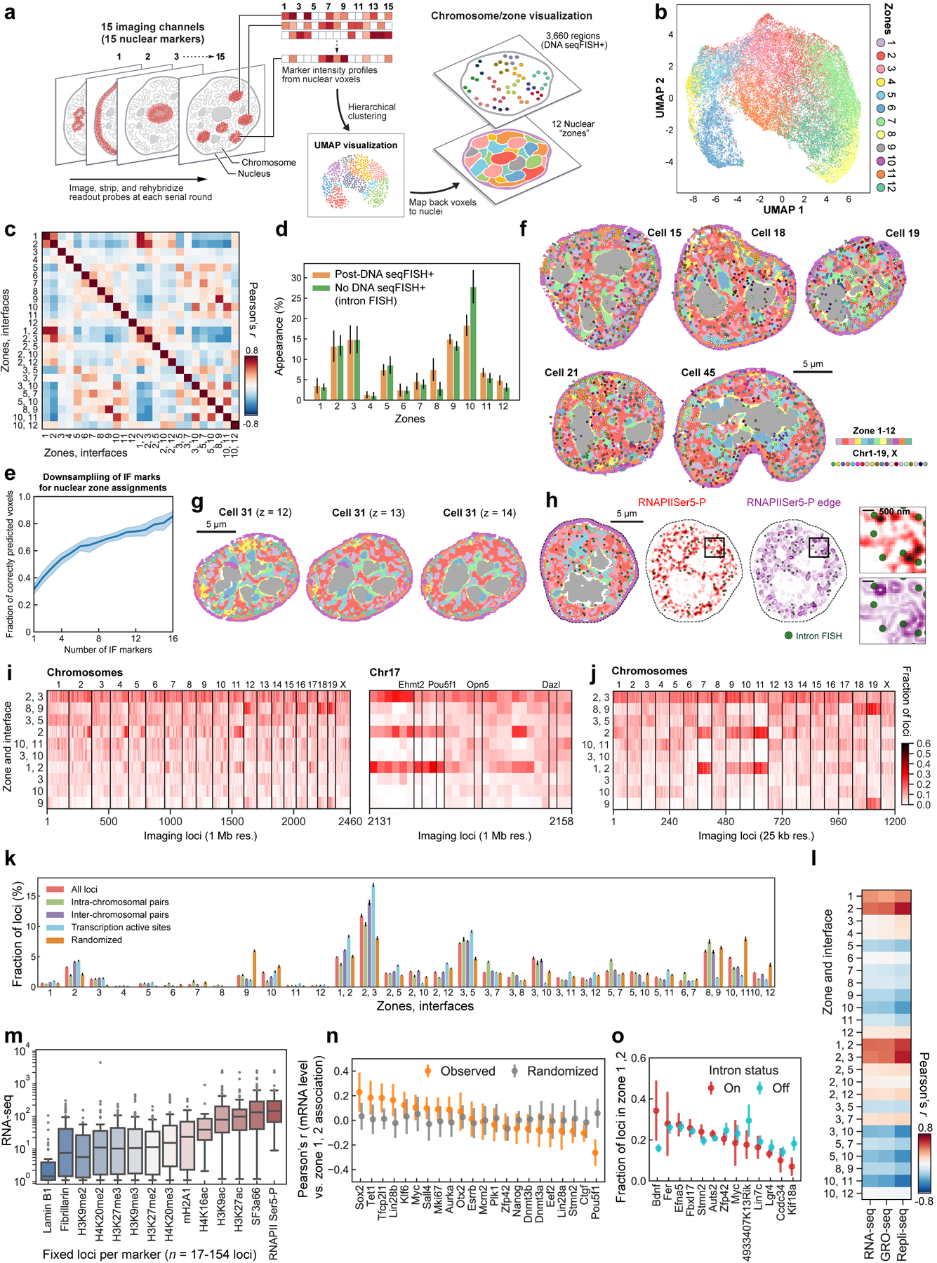
a, Analysis workflow for the pixel-based combinatorial chromatin profiling. Individual voxels with the 15 chromatin markers are clustered with hierarchical clustering and visually represented by a nonlinear dimensionality reduction technique, Uniform manifold approximation and projection (UMAP)⁷⁰. Voxels from individual clusters or “zones” are mapped back to individual nuclei, and overlaid with DNA seqFISH+ dots. b, UMAP representation for 44,000 pixels sampled from 201 cells, labeled with 12 zones. UMAP projection is used for visual clarity. c, Pearson correlation matrix between zones and interfaces based on the DNA loci association with zones and interfaces shown in f (n = 2,460 loci). Loci appearing in zone 1 are also more likely to be found in zone 2 as well as in interface 1/2. d, Comparison of zone appearance with and without DNA seqFISH+ treatment shows an overall agreement between the measurements. Mean values from 20 bootstrap trials are shown with error bars corresponding to standard errors. e, Assignment of zones as a function of downsampling of IF markers. 20 random subsets of IF markers are selected at each downsample size. The center of the curve reflects the mean and the width reflects the standard deviation of the correct zone assignments at each downsample size (see Methods). f, Reconstructions of zones and DNA loci in additional cells. g, Reconstructions of zones in the cell 31 with different z-planes. h, Reconstruction of zones and 1,000 gene intron dots as well as RNAPIISer5-P staining (background-subtracted) and edge of RNAPIISer5-P staining. i, Heatmap for probability of association between DNA loci, nuclear zones and interfaces for the 1 Mb data. Zones and interfaces are ordered according to the overall probability of association with DNA loci. Right panel shows the loci around Pou5f1 (Oct4) visualized in Fig. 3b (panel 1). Each locus in single cells is assigned to one zone or interface. The distribution shown in the heatmap reflects the single cell variability in zone association for each locus. For example, Ehmt2 and Pou5f1 (Oct4) loci were primarily associated with active zone 2 and interfaces 1/2 and 2/3, while Opn5 and Dazl loci were more uniformly distributed across many zones. j, Heatmap for probability of association between DNA loci, nuclear zones and interfaces for the 25 kb data. Loci within the same Mb region have similar nuclear zone and interface association probability. k, Frequency of association between DNA loci and zones/interfaces in single cells, calculated for all loci, loci with intra-chromosomal and interchromosomal pairs, transcription active sites measured by intron FISH, and random loci (randomized control). Mean values from 20 bootstrap trials are shown with error bars corresponding to standard errors. l, Correlation between zone association and gene expression levels (RNA-seq)⁴⁹, density of RNA polymerases on the loci (GRO-seq)⁷⁵ and early replication domains (Repli-seq)⁷⁶ for all loci at 1 Mb resolution (n = 2,460 loci). m, Expression levels of fixed loci for each IF marker from n = 446 cells. Population level expressions are taken from bulk RNAseq studies⁴⁹ and integrated for 1 Mb region. For the boxplots, the center line in the boxes marks median, the upper and lower limits of the boxes mark the interquartile range, the whiskers extend to the farthest data points within 1.5 times the interquartile range, and the gray points mark outliers. n, Correlation of mRNA levels and fraction of voxels within 300 nm of a given locus in single cells being in active zones for individual mRNAs. Mean values from 20 bootstrap trials are shown with error bars corresponding to standard errors for each mRNA. Randomized samples correspond to scrambling of mRNA and zone assignment values for each cell. o, Comparison of fraction of voxels within 300 nm of DNA loci to be in active zones (zone 1 and 2) for loci with an active intron signal (ON) versus loci with no intron signal (OFF) for individual introns. Mean values from 20 bootstrap trials are shown with error bars corresponding to standard errors. for each intronic RNA. n = 201 and 172 cells for DNA seqFISH+ and intron FISH measurements in b-l, n, o, respectively.

Extended Data Fig. 9 |. Heterogeneity of transcriptional and chromatin states and their relationships in single cells.

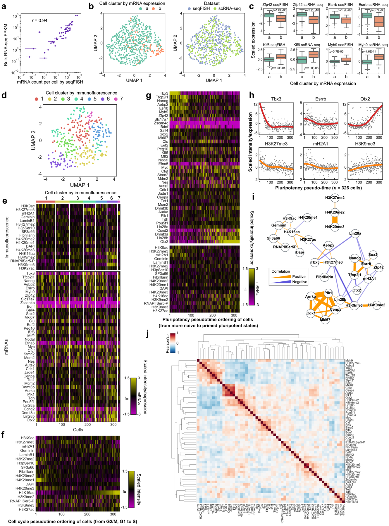
a, Pearson correlation of mean mRNA counts by RNA seqFISH and bulk RNA-seq. Error bars for RNA seqFISH represent the standard error of the mean from two measurements (n=151 and 175 cells from the center field of views). b, UMAP representation of individual cells in two different cell clusters identified based on scRNA-seq⁴² and mapped onto RNA seqFISH data (cluster a for cells with more pluripotent states and cluster b for cells on the differentiation path) (left), and in different datasets (right) (n = 326 and 250 cells for RNA seqFISH and scRNA-seq⁴² dataset, respectively). c, Boxplots showing a good agreement of differentially expressed genes in scRNA-seq and seqFISH datasets. p values were from a two-sided Wilcoxon’s rank sum test with cells in cluster a and b (n = 298 and 209 cells in cluster a and n = 28 and 41 cells in cluster b with RNA seqFISH and scRNA-seq⁴² dataset, respectively). For the boxplots, the center line in the boxes marks median, the upper and lower limits of the boxes mark the interquartile range, the whiskers extend to the farthest data points within 1.5 times the interquartile range, and the gray points mark outliers. d, UMAP representations of the cell clusters defined by IF intensity profiles. e, Heatmap of cell clusters with distinct IF profiles shown with cell cycle associated IF markers and all mRNA markers, similar to Fig. 4b. f, Pseudotime course analysis for cell cycle progression, cell cycle markers (H4K16ac, H4K20me1, H3pSer10) show clear enrichments while other markers do not show specific enrichments upon cell cycle pseudotime course, suggesting majority of the IF markers profiled are not primarily affected by cell cycle phases. g, Pseudotime course analysis for pluripotency states in mESCs based on scaled mRNA expression levels, showing the enrichment from markers associated with naive pluripotency such as Tfcp2l1 and Nanog to markers associated with primed pluripotency such as Dnmt3a, Lin28b and Otx2 as well as the enrichment of certain chromatin marks upon the pluripotency pseudotime course. h, Scaled marker gene expression (top panels) or intensity (bottom panels) along the pluripotency pseudotime ordering of cells. Raw data in g are overlaid with fitting curves (see Methods). i, Network analysis for the mRNA and immunofluorescence markers represents positive and negative Pearson correlation relationships among markers. j, Joint Pearson correlation matrix between mRNA and IF markers based on the scaled expression or intensity profiles in single cells (n = 41 mRNA and 25 IF markers). n = 326 cells in the center field of views for RNA seqFISH and IF data in a-j.

Extended Data Fig. 10 |. Additional analysis for colony level cell state heterogeneity.

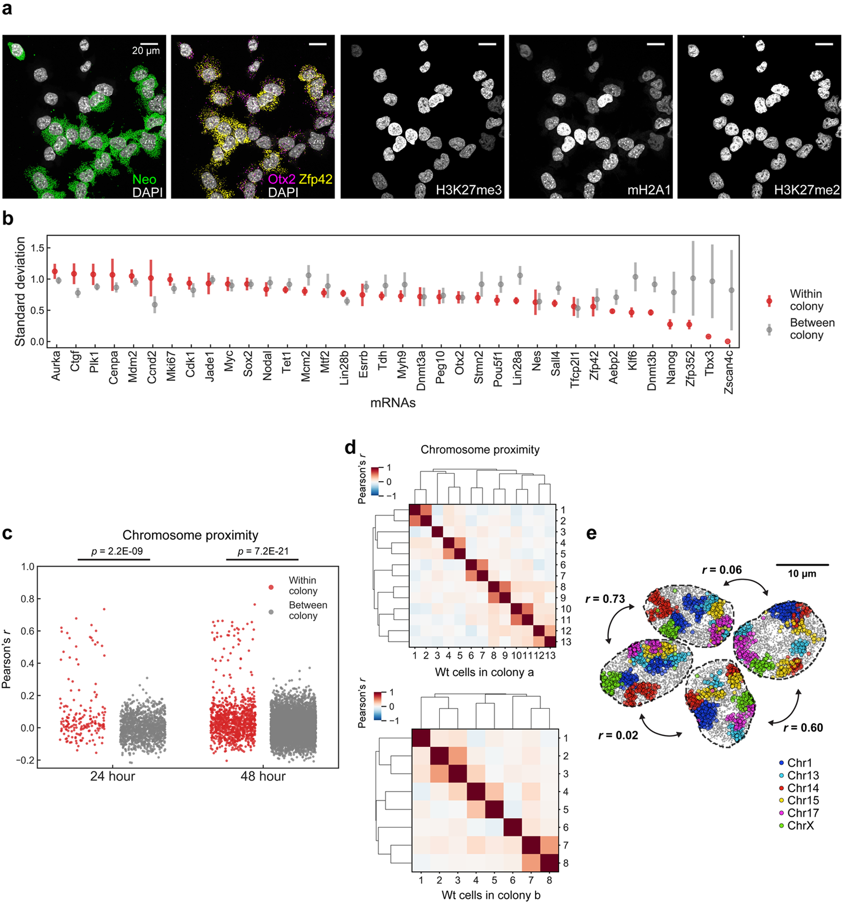
a, mRNA and IF images in a colony in the 48 hour clonal tracing experiment. H3K27me3 and mH2A1 overall intensities are similar in WT cells (GFP/Neo negative) in the colony. b, Standard deviation of normalized mRNA levels within colonies (red) and between colonies (grey). Error bars are standard errors for 20 bootstrap trials. Tbx3 and Nanog are more homogeneous within colonies, consistent with previous findings of the long-lived transcriptional states of these genes across several generations by single cell live imaging experiments^41,49. n = 117 unlabeled cells within colonies from a 48-hour dataset. c, Histogram of cell-to-cell correlations of chromosome to chromosome proximity maps for cells within colonies (red) and between colonies (grey). Cells with similar chromosome structures (red dots with high correlation values) are likely to be sister cells. Y-axis represents Pearson correlation coefficient, computed by 20 × 20 chromosome proximity matrices from pairs of cells. p values were from a two-sided Wilcoxon’s rank sum test with pairs of cells of 180, 1,198, 966 and 5,820 (from left to right). d, Correlation of chromosome proximities between cells in colonies in the 48 hour clonal tracing experiment. Strong correlations are seen between putative sister cells suggesting that gross chromosome proximities are preserved for 1 generation. Color bars represent Pearson correlation coefficient computed in c. e, Chromosome images for unlabeled cells from a 24-hour colony shows similarities between two sets of neighboring cells (maximum z projection). Chromosome organizations in single cells are highly correlated between pairs of cells that were physically close, possibly sister cells, and are mostly uncorrelated with other cells in the colonies. 6 chromosomes are shown for visual clarity. r represents Pearson correlation coefficient computed in c.

References

- 1.Dekker J et al. The 4D nucleome project. Nature 549, 219–226 (2017). [DOI] [PMC free article] [PubMed] [Google Scholar]
- 2.Kelsey G, Stegle O & Reik W Single-cell epigenomics: Recording the past and predicting the future. Science vol. 358 69–75 (2017). [DOI] [PubMed] [Google Scholar]
- 3.Kempfer R & Pombo A Methods for mapping 3D chromosome architecture. Nat. Rev. Genet 21, 207–226 (2020). [DOI] [PubMed] [Google Scholar]
- 4.Zhu C, Preissl S & Ren B Single-cell multimodal omics: the power of many. Nat. Methods 17, 11–14 (2020). [DOI] [PubMed] [Google Scholar]
- 5.Finn EH & Misteli T Molecular basis and biological function of variability in spatial genome organization. Science 365, (2019). [DOI] [PMC free article] [PubMed] [Google Scholar]
- 6.Lieberman-Aiden E et al. Comprehensive mapping of long-range interactions reveals folding principles of the human genome. Science 326, 289–293 (2009). [DOI] [PMC free article] [PubMed] [Google Scholar]
- 7.Quinodoz SA et al. Higher-Order Inter-chromosomal Hubs Shape 3D Genome Organization in the Nucleus. Cell 174, 744–757.e24 (2018). [DOI] [PMC free article] [PubMed] [Google Scholar]
- 8.Wang S et al. Spatial organization of chromatin domains and compartments in single chromosomes. Science 353, 598–602 (2016). [DOI] [PMC free article] [PubMed] [Google Scholar]
- 9.Bintu B et al. Super-resolution chromatin tracing reveals domains and cooperative interactions in single cells. Science 362, (2018). [DOI] [PMC free article] [PubMed] [Google Scholar]
- 10.Nir G et al. Walking along chromosomes with super-resolution imaging, contact maps, and integrative modeling. PLoS Genet. 14, e1007872 (2018). [DOI] [PMC free article] [PubMed] [Google Scholar]
- 11.Cardozo Gizzi AM et al. Microscopy-Based Chromosome Conformation Capture Enables Simultaneous Visualization of Genome Organization and Transcription in Intact Organisms. Mol. Cell 74, 212–222.e5 (2019). [DOI] [PubMed] [Google Scholar]
- 12.Finn EH et al. Extensive Heterogeneity and Intrinsic Variation in Spatial Genome Organization. Cell 176, 1502–1515.e10 (2019). [DOI] [PMC free article] [PubMed] [Google Scholar]
- 13.Mateo LJ et al. Visualizing DNA folding and RNA in embryos at single-cell resolution. Nature 568, 49–54 (2019). [DOI] [PMC free article] [PubMed] [Google Scholar]
- 14.Nguyen HQ et al. 3D mapping and accelerated super-resolution imaging of the human genome using in situ sequencing. Nat. Methods 17, 822–832 (2020). [DOI] [PMC free article] [PubMed] [Google Scholar]
- 15.Su J-H, Zheng P, Kinrot SS, Bintu B & Zhuang X Genome-Scale Imaging of the 3D Organization and Transcriptional Activity of Chromatin. Cell 182, 1641–1659.e26 (2020). [DOI] [PMC free article] [PubMed] [Google Scholar]
- 16.Beliveau BJ et al. Versatile design and synthesis platform for visualizing genomes with Oligopaint FISH probes. Proc. Natl. Acad. Sci. U. S. A 109, 21301–21306 (2012). [DOI] [PMC free article] [PubMed] [Google Scholar]
- 17.Lubeck E, Coskun AF, Zhiyentayev T, Ahmad M & Cai L Single-cell in situ RNA profiling by sequential hybridization. Nature methods vol. 11 360–361 (2014). [DOI] [PMC free article] [PubMed] [Google Scholar]
- 18.Shah S, Lubeck E, Zhou W & Cai L In Situ Transcription Profiling of Single Cells Reveals Spatial Organization of Cells in the Mouse Hippocampus. Neuron 92, 342–357 (2016). [DOI] [PMC free article] [PubMed] [Google Scholar]
- 19.Takei Y, Shah S, Harvey S, Qi LS & Cai L Multiplexed Dynamic Imaging of Genomic Loci by Combined CRISPR Imaging and DNA Sequential FISH. Biophys. J 112, 1773–1776 (2017). [DOI] [PMC free article] [PubMed] [Google Scholar]
- 20.Shah S et al. Dynamics and Spatial Genomics of the Nascent Transcriptome by Intron seqFISH. Cell 174, 363–376.e16 (2018). [DOI] [PMC free article] [PubMed] [Google Scholar]
- 21.Eng C-HL et al. Transcriptome-scale super-resolved imaging in tissues by RNA seqFISH+. Nature 568, 235–239 (2019). [DOI] [PMC free article] [PubMed] [Google Scholar]
- 22.Chen KH, Boettiger AN, Moffitt JR, Wang S & Zhuang X RNA imaging. Spatially resolved, highly multiplexed RNA profiling in single cells. Science 348, aaa6090 (2015). [DOI] [PMC free article] [PubMed] [Google Scholar]
- 23.Bonev B et al. Multiscale 3D Genome Rewiring during Mouse Neural Development. Cell 171, 557–572.e24 (2017). [DOI] [PMC free article] [PubMed] [Google Scholar]
- 24.Shen Y et al. A map of the cis-regulatory sequences in the mouse genome. Nature 488, 116–120 (2012). [DOI] [PMC free article] [PubMed] [Google Scholar]
- 25.Boettiger AN et al. Super-resolution imaging reveals distinct chromatin folding for different epigenetic states. Nature 529, 418–422 (2016). [DOI] [PMC free article] [PubMed] [Google Scholar]
- 26.van Steensel B & Belmont AS Lamina-Associated Domains: Links with Chromosome Architecture, Heterochromatin, and Gene Repression. Cell 169, 780–791 (2017). [DOI] [PMC free article] [PubMed] [Google Scholar]
- 27.Spector DL & Lamond AI Nuclear speckles. Cold Spring Harb. Perspect. Biol 3, (2011). [DOI] [PMC free article] [PubMed] [Google Scholar]
- 28.Pederson T The nucleolus. Cold Spring Harb. Perspect. Biol 3, (2011). [DOI] [PMC free article] [PubMed] [Google Scholar]
- 29.Ludwig CH & Bintu L Mapping chromatin modifications at the single cell level. Development 146, (2019). [DOI] [PMC free article] [PubMed] [Google Scholar]
- 30.Söderberg O et al. Direct observation of individual endogenous protein complexes in situ by proximity ligation. Nat. Methods 3, 995–1000 (2006). [DOI] [PubMed] [Google Scholar]
- 31.Agasti SS et al. DNA-barcoded labeling probes for highly multiplexed Exchange-PAINT imaging. Chem. Sci 8, 3080–3091 (2017). [DOI] [PMC free article] [PubMed] [Google Scholar]
- 32.Guenatri M, Bailly D, Maison C & Almouzni G Mouse centric and pericentric satellite repeats form distinct functional heterochromatin. J. Cell Biol 166, 493–505 (2004). [DOI] [PMC free article] [PubMed] [Google Scholar]
- 33.Solovei I et al. Nuclear architecture of rod photoreceptor cells adapts to vision in mammalian evolution. Cell 137, 356–368 (2009). [DOI] [PubMed] [Google Scholar]
- 34.Mao YS, Zhang B & Spector DL Biogenesis and function of nuclear bodies. Trends Genet. 27, 295–306 (2011). [DOI] [PMC free article] [PubMed] [Google Scholar]
- 35.Peric-Hupkes D et al. Molecular maps of the reorganization of genome-nuclear lamina interactions during differentiation. Mol. Cell 38, 603–613 (2010). [DOI] [PMC free article] [PubMed] [Google Scholar]
- 36.Kind J et al. Genome-wide maps of nuclear lamina interactions in single human cells. Cell 163, 134–147 (2015). [DOI] [PMC free article] [PubMed] [Google Scholar]
- 37.Chen Y et al. Mapping 3D genome organization relative to nuclear compartments using TSA-Seq as a cytological ruler. J. Cell Biol 217, 4025–4048 (2018). [DOI] [PMC free article] [PubMed] [Google Scholar]
- 38.Gut G, Herrmann MD & Pelkmans L Multiplexed protein maps link subcellular organization to cellular states. Science 361, (2018). [DOI] [PubMed] [Google Scholar]
- 39.McSwiggen DT, Mir M, Darzacq X & Tjian R Evaluating phase separation in live cells: diagnosis, caveats, and functional consequences. Genes Dev. 33, 1619–1634 (2019). [DOI] [PMC free article] [PubMed] [Google Scholar]
- 40.Marks H et al. The transcriptional and epigenomic foundations of ground state pluripotency. Cell 149, 590–604 (2012). [DOI] [PMC free article] [PubMed] [Google Scholar]
- 41.Singer ZS et al. Dynamic heterogeneity and DNA methylation in embryonic stem cells. Mol. Cell 55, 319–331 (2014). [DOI] [PMC free article] [PubMed] [Google Scholar]
- 42.Kolodziejczyk AA et al. Single Cell RNA-Sequencing of Pluripotent States Unlocks Modular Transcriptional Variation. Cell Stem Cell 17, 471–485 (2015). [DOI] [PMC free article] [PubMed] [Google Scholar]
- 43.Tosolini M et al. Contrasting epigenetic states of heterochromatin in the different types of mouse pluripotent stem cells. Sci. Rep 8, 5776 (2018). [DOI] [PMC free article] [PubMed] [Google Scholar]
- 44.van Mierlo G et al. Integrative Proteomic Profiling Reveals PRC2-Dependent Epigenetic Crosstalk Maintains Ground-State Pluripotency. Cell Stem Cell 24, 123–137.e8 (2019). [DOI] [PubMed] [Google Scholar]
- 45.Gerlich D et al. Global chromosome positions are transmitted through mitosis in mammalian cells. Cell 112, 751–764 (2003). [DOI] [PubMed] [Google Scholar]
- 46.Walter J, Schermelleh L, Cremer M, Tashiro S & Cremer T Chromosome order in HeLa cells changes during mitosis and early G1, but is stably maintained during subsequent interphase stages. J. Cell Biol 160, 685–697 (2003). [DOI] [PMC free article] [PubMed] [Google Scholar]
- 47.Thomson I, Gilchrist S, Bickmore WA & Chubb JR The Radial Positioning of Chromatin Is Not Inherited through Mitosis but Is Established De Novo in Early G1. Curr. Biol 14, 166–172 (2004). [DOI] [PubMed] [Google Scholar]
- 48.Essers J et al. Dynamics of relative chromosome position during the cell cycle. Mol. Biol. Cell 16, 769–775 (2005). [DOI] [PMC free article] [PubMed] [Google Scholar]
- 49.Hormoz S et al. Inferring Cell-State Transition Dynamics from Lineage Trees and Endpoint Single-Cell Measurements. Cell Syst 3, 419–433.e8 (2016). [DOI] [PMC free article] [PubMed] [Google Scholar]
- 50.Cunningham F et al. Ensembl 2019. Nucleic Acids Res. 47, D745–D751 (2019). [DOI] [PMC free article] [PubMed] [Google Scholar]
- 51.Klein AM et al. Droplet barcoding for single-cell transcriptomics applied to embryonic stem cells. Cell 161, 1187–1201 (2015). [DOI] [PMC free article] [PubMed] [Google Scholar]
- 52.Langmead B & Salzberg SL Fast gapped-read alignment with Bowtie 2. Nat. Methods 9, 357–359 (2012). [DOI] [PMC free article] [PubMed] [Google Scholar]
- 53.Camacho C et al. BLAST+: architecture and applications. BMC Bioinformatics 10, 421 (2009). [DOI] [PMC free article] [PubMed] [Google Scholar]
- 54.Bao W, Kojima KK & Kohany O Repbase Update, a database of repetitive elements in eukaryotic genomes. Mob. DNA 6, 11 (2015). [DOI] [PMC free article] [PubMed] [Google Scholar]
- 55.Eng C-HL, Shah S, Thomassie J & Cai L Profiling the transcriptome with RNA SPOTs. Nat. Methods 14, 1153–1155 (2017). [DOI] [PMC free article] [PubMed] [Google Scholar]
- 56.Cremer C et al. Principles of spectral precision distance confocal microscopy for the analysis of molecular nuclear structure. Handbook of computer vision and applications 3, 839–857 (1999). [Google Scholar]
- 57.Croft JA et al. Differences in the localization and morphology of chromosomes in the human nucleus. J. Cell Biol 145, 1119–1131 (1999). [DOI] [PMC free article] [PubMed] [Google Scholar]
- 58.Esa A et al. Three-dimensional spectral precision distance microscopy of chromatin nanostructures after triple-colour DNA labelling: a study of the BCR region on chromosome 22 and the Philadelphia chromosome. J. Microsc 199, 96–105 (2000). [DOI] [PubMed] [Google Scholar]
- 59.Cremer M et al. Multicolor 3D fluorescence in situ hybridization for imaging interphase chromosomes. Methods Mol. Biol 463, 205–239 (2008). [DOI] [PubMed] [Google Scholar]
- 60.Zhang Z, Revyakin A, Grimm JB, Lavis LD & Tjian R Single-molecule tracking of the transcription cycle by sub-second RNA detection. Elife 3, e01775 (2014). [DOI] [PMC free article] [PubMed] [Google Scholar]
- 61.Chen B et al. Dynamic imaging of genomic loci in living human cells by an optimized CRISPR/Cas system. Cell 155, 1479–1491 (2013). [DOI] [PMC free article] [PubMed] [Google Scholar]
- 62.Nilsson M et al. Padlock probes: circularizing oligonucleotides for localized DNA detection. Science 265, 2085–2088 (1994). [DOI] [PubMed] [Google Scholar]
- 63.Rouhanifard SH et al. ClampFISH detects individual nucleic acid molecules using click chemistry-based amplification. Nat. Biotechnol (2018) doi: 10.1038/nbt.4286. [DOI] [PMC free article] [PubMed] [Google Scholar]
- 64.Edelstein A, Amodaj N, Hoover K, Vale R & Stuurman N Computer control of microscopes using μManager. Curr. Protoc. Mol. Biol Chapter 14, Unit14.20 (2010). [DOI] [PMC free article] [PubMed] [Google Scholar]
- 65.Liu S-L et al. Fast and high-accuracy localization for three-dimensional single-particle tracking. Sci. Rep 3, 2462 (2013). [DOI] [PMC free article] [PubMed] [Google Scholar]
- 66.Parthasarathy R Rapid, accurate particle tracking by calculation of radial symmetry centers. Nat. Methods 9, 724–726 (2012). [DOI] [PubMed] [Google Scholar]
- 67.Durand NC et al. Juicer Provides a One-Click System for Analyzing Loop-Resolution Hi-C Experiments. Cell Syst 3, 95–98 (2016). [DOI] [PMC free article] [PubMed] [Google Scholar]
- 68.Knight PA & Ruiz D A fast algorithm for matrix balancing. IMA J. Numer. Anal 33, 1029–1047 (2013). [Google Scholar]
- 69.Stanyte R et al. Dynamics of sister chromatid resolution during cell cycle progression. J. Cell Biol 217, 1985–2004 (2018). [DOI] [PMC free article] [PubMed] [Google Scholar]
- 70.McInnes L, Healy J, Saul N & Großberger L UMAP: Uniform Manifold Approximation and Projection. Journal of Open Source Software vol. 3 861 (2018). [Google Scholar]
- 71.Nmezi B et al. Concentric organization of A- and B-type lamins predicts their distinct roles in the spatial organization and stability of the nuclear lamina. Proc. Natl. Acad. Sci. U. S. A 116, 4307–4315 (2019). [DOI] [PMC free article] [PubMed] [Google Scholar]
- 72.Suzuki H, Kurihara Y, Kanehisa T & Moriwaki K Variation in the distribution of silver-staining nucleolar organizer regions on the chromosomes of the wild mouse, Mus musculus. Mol. Biol. Evol 7, 271–282 (1990). [DOI] [PubMed] [Google Scholar]
- 73.Kurihara Y, Suh DS, Suzuki H & Moriwaki K Chromosomal locations of Ag-NORs and clusters of ribosomal DNA in laboratory strains of mice. Mamm. Genome 5, 225–228 (1994). [DOI] [PubMed] [Google Scholar]
- 74.Strongin DE, Groudine M & Politz JCR Nucleolar tethering mediates pairing between the IgH and Myc loci. Nucleus 5, 474–481 (2014). [DOI] [PMC free article] [PubMed] [Google Scholar]
- 75.Jonkers I, Kwak H & Lis JT Genome-wide dynamics of Pol II elongation and its interplay with promoter proximal pausing, chromatin, and exons. Elife 3, e02407 (2014). [DOI] [PMC free article] [PubMed] [Google Scholar]
- 76.Dileep V & Gilbert DM Single-cell replication profiling to measure stochastic variation in mammalian replication timing. Nat. Commun 9, 427 (2018). [DOI] [PMC free article] [PubMed] [Google Scholar]
- 77.Bacher R et al. SCnorm: robust normalization of single-cell RNA-seq data. Nat. Methods 14, 584–586 (2017). [DOI] [PMC free article] [PubMed] [Google Scholar]
- 78.Vallejos CA, Risso D, Scialdone A, Dudoit S & Marioni JC Normalizing single-cell RNA sequencing data: challenges and opportunities. Nat. Methods 14, 565–571 (2017). [DOI] [PMC free article] [PubMed] [Google Scholar]
- 79.Hafemeister C & Satija R Normalization and variance stabilization of single-cell RNA-seq data using regularized negative binomial regression. Genome Biol. 20, 296 (2019). [DOI] [PMC free article] [PubMed] [Google Scholar]
- 80.Traag VA, Waltman L & van Eck NJ From Louvain to Leiden: guaranteeing well-connected communities. Sci. Rep 9, 5233 (2019). [DOI] [PMC free article] [PubMed] [Google Scholar]
- 81.Stuart T et al. Comprehensive Integration of Single-Cell Data. Cell 177, 1888–1902.e21 (2019). [DOI] [PMC free article] [PubMed] [Google Scholar]
- 82.Serrano L et al. The tumor suppressor SirT2 regulates cell cycle progression and genome stability by modulating the mitotic deposition of H4K20 methylation. Genes Dev. 27, 639–653 (2013). [DOI] [PMC free article] [PubMed] [Google Scholar]
- 83.Hastie T & Stuetzle W Principal Curves. Journal of the American Statistical Association vol. 84 502–516 (1989). [Google Scholar]
- 84.Haghverdi L, Büttner M, Wolf FA, Buettner F & Theis FJ Diffusion pseudotime robustly reconstructs lineage branching. Nat. Methods 13, 845–848 (2016). [DOI] [PubMed] [Google Scholar]
- 85.van Dijk D et al. Recovering Gene Interactions from Single-Cell Data Using Data Diffusion. Cell 174, 716–729.e27 (2018). [DOI] [PMC free article] [PubMed] [Google Scholar]
- 86.Angerer P et al. destiny: diffusion maps for large-scale single-cell data in R. Bioinformatics 32, 1241–1243 (2016). [DOI] [PubMed] [Google Scholar]
- 87.Shannon P et al. Cytoscape: a software environment for integrated models of biomolecular interaction networks. Genome Res. 13, 2498–2504 (2003). [DOI] [PMC free article] [PubMed] [Google Scholar]
- 88.Lyon MF X-chromosome inactivation: a repeat hypothesis. Cytogenet. Cell Genet 80, 133–137 (1998). [DOI] [PubMed] [Google Scholar]
- 89.Meuleman W et al. Constitutive nuclear lamina-genome interactions are highly conserved and associated with A/T-rich sequence. Genome Research vol. 23 270–280 (2013). [DOI] [PMC free article] [PubMed] [Google Scholar]
Associated Data
This section collects any data citations, data availability statements, or supplementary materials included in this article.