Do human butchery patterns exist? A study of the interaction of randomness and channelling in the distribution of cut marks on long bones

Abstract

Bone surface modifications (BSMs) in faunal assemblages are frequently used to infer past agency and actions of hominins and carnivores, with implications for the emergence of key human behaviours. Patterning of BSMs has mostly been defined as a combination of the intensity of marks per bone portion and sometimes per element. Numerous variables involved in butchery can condition cut mark anatomical distribution, so much so that these variables are widely assumed to be stochastic. Here, we present a new methodological approach using a novel geospatial tool (Ikhnos) which combines the three-dimensional spatial documentation of cut mark patterns with spatial statistics based on wavelets, applied to three experimental and ethnoarchaeological faunal assemblages. We use wavelets to identify patterning of multiple longitudinal series of cut mark distributions on bones, and to establish similarities or differences in patterning within and across different assemblages. This method demonstrates the existence of general and behaviour-specific butchery patterns. It can also be used to effectively assess the proportion of mark clustering that is due to randomness, versus that which is conditioned by the butchery process.

1. Introduction

Cut marks, a type of anthropogenic bone surface modification (BSM), have commonly been interpreted as unintentional ‘accidents’ whose traces were left on bones during butchery by humans or hominin ancestors [1,2]. This assumption hinders any systematic interpretation of butchered animal remains, because it suggests that the stochastic, unpredictable element of purported ‘butchery patterns’ overrides any structural regularity in them. For example, Lyman writes:

If butchery marks are epiphenomena, that is, they are in some sense an unintended, accidental, fortuitous, or incidental result of butchery activities, then frequencies of butchered bones are potentially ambiguous indicators of the quantitative aspects of human behaviors, and thus terms such as ‘butchery pattern’ would be inappropriate given its human behavioral implications [3, p. 301].

Taphonomists are aware that multiple variables contribute to the process of butchery and the resulting cut marks on bones. Some of the most relevant are: the number of butchers involved and their experience, tool raw material (e.g. metal versus stone), tool type (e.g. simple or retouched flakes) and butchery goals (e.g. dismembering, filleting) [4–9]. Some of these variables have been experimentally shown to produce different cut mark frequencies in faunal assemblages [10–13]. These factors, among others, have prompted some researchers to diminish or exclude the potential information that can be obtained from analysing cut marks when targeting carnivore–hominin interactions [14–16]. But are cut marks on bones random accidents which, therefore, are spatially random? Should they reflect this by adopting spatial randomness as in Poisson point processes? Or, are there patterns behind the apparent high variability in cut marks, which are created by specific constraining factors during butchery? If so, then the determination of these patterns could potentially reveal the interplay of some or even all of the aforementioned variables in the butchery process [17].

The problem is not limited to cut marks. Tooth marks inflicted by carnivores, especially those of strictly flesh-eating predators who try to avoid contact with bone (such as felids), should also be considered to be accidents. Therefore, they should be randomly distributed on bones. However, multiple studies of bone modification patterns by felids reveal that tooth marks on long bones do indeed exhibit trends, clustering mainly in some locations and not others [18], which make faunal assemblages tooth-marked by felids [18,19] differentiable from those modified by canids [20,21] and by hyenids [22]. Thus, studies with carnivores show that contingency does not produce randomness in mark location, but rather it mainly impacts mark intensity (i.e. frequency).

This could also be the case for cut marks. Butchery patterns have been argued to exist when comparing experimental assemblages simulating primary access to carcasses by humans, versus secondary access wherein humans access carcasses only after carnivores have intervened [23–25]. These patterns have been explained by the fact that after felids consume carcasses, they leave behind scraps of flesh on bones in specific anatomical locations, enabling researchers to define ‘hot’ and ‘cold’ zones on bones that may be more or less likely to preserve specific BSM [24]. Determination of butchery patterns such as these is necessary if we aim to successfully address some of the most important questions in the taphonomy of palaeoanthropological and archaeological sites: how and in what state were carcasses acquired by hominins? How were these carcasses dismembered, defleshed and ultimately consumed? Can the effects of variation in butcher experience, tool types, or any of the other variables discussed above be detected and interpreted? Are there cultural differences in butchery practices across different groups of people? [17,26–29].

As in the case of tooth marks, the key elements in determining cut mark patterns are mark location and mark intensity. Repeated modification of bones in the same loci implies a non-random phenomenon. Consideration of the whole ensemble of BSM loci on a bone and, by extension, on all bone types in any given skeletal assemblage, is what constitutes a pattern. Intensity varies more widely and is more sensitive to stochasticity. For example, expert butchers may leave fewer cut marks than novice butchers since they should have fewer ‘accidents.’ However, both experienced and inexperienced butchers may leave marks in greater proportion (i.e. clustering) in specific spots. These spots may be conditioned by carcass muscle, tendon and ligament insertions and by other factors [1,10,11,30,31].

In this study, we develop and apply a statistical method aimed at determining the proportion of stochastic cut marks (highly variable in their location and frequencies) versus those created systematically under more patterned processes. Applying this method to three experimental and ethnoarchaeological samples, we seek to address the following questions:

• 1. Is there any statistically significant patterning produced during butchery in the distribution of cut marks on all meat-bearing long bones, or are the marks distributed randomly?

• 2. Is there patterning only in certain skeletal elements, caused by specific muscle locations and the ergonomics of stone tool use during butchery?

• 3. Can different types of human access to carcasses (primary versus secondary) be documented through behaviour-specific cutmarking patterns?

• 4. Can butchery patterns in whole assemblages be compared against those of other assemblages, in order to quantitatively establish degrees of inter-assemblage difference?

Our results highlight the locations where patterns emerge and we provide analytical tools that enable taphonomists to compare inter-assemblage BSM variability and distances and to relate these inter-assemblage differences to specific behaviours. This study shows that, despite the high variability of archaeologists' subjective assessments of frequencies and distributions of cut marks, cutmarking patterns do exist, and these can be linked to specific behaviours. These findings have implications for the interpretation of some of the most important palaeoanthropological sites for the study of human origins, but can equally be applied to later periods of human history.

2. Sample and methods

2.1. Experimental and ethnoarchaeological faunal samples

Three experimental and ethnoarchaeological assemblages were chosen in order to sample different butchery scenarios. For the butchery of complete carcasses, we used the four sheep carcasses reported in the experiment conducted by Domínguez-Rodrigo & Barba [32]. These were butchered by students, with no prior experience, using chert and quartzite simple flakes. The assemblage of broken long bones included 401 specimens (table 1). The students were divided into four groups with each carcass being butchered by three people. Bones were subsequently cleaned with neutral detergent, and marks were identified to bone portion and element with the aid of 10×–20× hand lenses. There was substantial variability in the frequency and anatomical distribution of cut marks, resulting from the variable degrees of experience and skills and the groupings of these novice butchers [32]. For the present analysis, we use only the five meat-bearing long bones (humerus, femur, radius-ulna and tibia); for cut mark distribution frequencies per element and carcass, see [32].

Table 1.

Number of specimens (NISP) according to element and side (with number of cutmarked fragments in parentheses) from the experimental bucthery assemblage. Total refers to the percentage of specimens of each element cutmarked.

element	left side	right side	total	total (%)
femur	40 (9)	45 (15)	85 (24)	28.2
humerus	43 (13)	50 (16)	93 (29)	31.2
tibia	61 (18)	61 (20)	122 (38)	31.1
radio-ulna	52 (13)	49 (14)	101 (27)	26.7

As a comparative framework that was not experimentally conditioned, we used an assemblage collected in 2006 at Sonai Rockshelter, northeast of Lake Eyasi in Tanzania [33] (figure 1). During archaeological fieldwork in 2005, we were taken to the site by Hadza informants, who said that they had used it in recent years, although pastoralists also lived nearby and may have used the shelter occasionally. During 1997 surveys, Hadza were also occupying the shelter (A.Z.P. Mabulla 2005, personal communication). In 2005, we saw fresh-appearing hearths and garbage inside the shelter, and numerous bones in a wide discard area in front of it and downslope, mainly clustered underneath bushes. Upon returning to conduct archaeological excavations in 2006 and after receiving permission from informants to do so, a complete surface collection was made, dividing the discard area into five collection zones [33].

Figure 1.

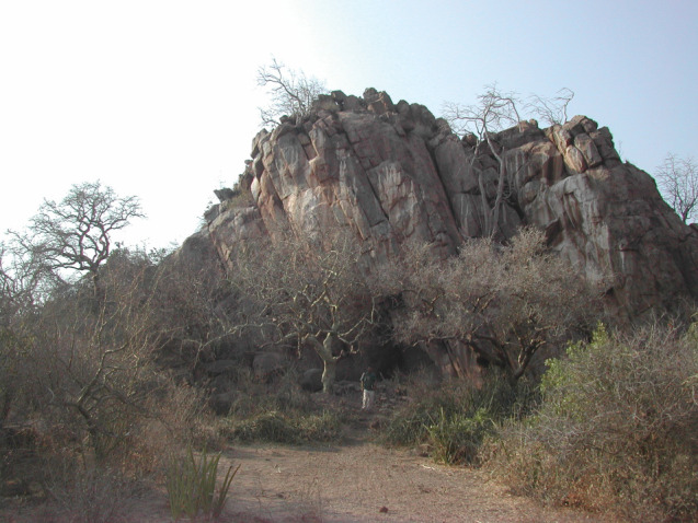
Sonai Rockshelter, northeast of Lake Eyasi, Tanzania. The surface faunal collection was found primarily in front of and downslope from the shelter.

While the bones collected on the surface were fully skeletonized, they were strikingly different from those eroding out of the shelter's archaeological deposits, in that the surface-collected bones were neither mineralized nor coated in calcium carbonate. This quality of preservation, together with associated late twentieth- to early twenty-first-century material culture such as coins, plastic beads, plastic buttons and metal scraps, suggests a recent formation date for the surface assemblage. Given, however, that we do not know the temporal span of the assemblage, nor did we witness its formation, we cautiously refer to the surface assemblage as a modern butchery assemblage, without assumptions about the economic or social identities of the butchers as foragers or pastoralists, nor about the number or duration of events that led to its formation. We do, however, assume that butchery involved much more experienced butchers than those in the experiment described above. We assume that butchery took place with metal knives, given the twentieth-century origins of the assemblage and the widespread use of metal knives in Hadza communities for decades to centuries [34]. Metal implements generate cut marks that are easily distinguishable from those inflicted with stone flakes on bones. Our assessment of the cut marks in the Sonai assemblage confirms that they were made with metal tools.

The surface assemblage is large (NISP = 1223) and diverse (14 taxa identified), and includes ungulates (bovids and equids), primates (baboon and monkey), as well as smaller mammals (hyrax) and reptiles (tortoise) (electronic supplementary material). Wild bovids include dik-dik, bush duiker, gazelle and kudu, but livestock (cattle, caprines and a donkey) form nearly 40% of the total minimum number of individuals (MNI). For the present study, we focus only on the five meat-bearing bones listed above, from the ungulate and ungulate-sized appendicular subsample of the surface assemblage (NISP = 146) (table 2).

Table 2.

Number of specimens (NISP) according to element and side (with number of cutmarked fragments in parentheses) from the Sonai ethnoarchaeological assemblage. Total refers to the percentage of specimens of each element cutmarked.

element	left side	right side	total	total (%)
femur	14 (4)	18(8)	32 (12)	37.5
humerus	14 (2)	32 (20)	46 (22)	47.8
tibia	22 (7)	18 (8)	40 (15)	37.5
radio-ulna	12 (3)	16 (12)	28 (15)	53.6

Finally, a third sample is composed of 10 carcasses obtained at lion kills in Tarangire National Park in Tanzania, used for modelling BSM distribution in scenarios of passive scavenging from felid kills by hominins [35] (table 3). These carcasses were obtained at kills and had been substantially or mostly defleshed upon abandonment by lions. The remaining bulk flesh and scraps were removed using quartzite stone tools (simple flakes). A summary of sample composition and methodology is provided by Gidna [35]. The carcasses used from the Tarangire sample are medium-sized and were marginally cutmarked (tables 3 and 4). This made them an appropriate comparison to the smaller sheep carcasses butchered in the student experiment, because medium-sized carcasses retain more flesh scraps after felid consumption than smaller carcasses, and their subsequent butchery is, therefore, prone to generate more cut marks. The use of this sample in this study was not aimed at describing a butchery model of scavenged carcasses, but rather to show that this model exists and that it can be differentiated from other patterned models.

Table 3.

Zebra and wildebeest carcasses analysed in the present study, including the number of lion consumers.

carcass no.	habitat	prey	no. lions
2	bush	wildebeest	7
4	bush	zebra	7
5	bush	zebra	4
6	forest	zebra	4
7	forest	zebra	4
8	plain	wildebeest	7
9	forest	wildebeest	2
10	forest	wildebeest	2
11	forest	zebra	2
12	forest	wildebeest	7

Table 4.

Number of cutmarked bones and total number of elements from the Tarangire sample.

element	no. cm_bones	total elements
humerus	3	20
femur	2	20
radius-ulna	17	20
tibia	5	20

Given that the null hypothesis was that the interplay of highly variable experimental scenarios will produce higher random variability in the resulting cut mark patterns, the mixing of different animal sizes, raw materials for butchering tools (stone and metal), as well as the diverse degrees of expertize of the butchers involved (novice students and experienced foragers) was intentional for the purpose of efficiently testing the hypothesis that cutmarking results from stochastic contingency.

2.2. Methods of statistical analysis

For all three samples, BSM (cut marks, tooth marks and percussion marks) were observed on each long bone using 10–20× hand lenses and were identified in their precise location on the skeletal element. These locations were recorded on three-dimensional templates of each skeletal element using IKHNOS, a software specifically designed to record BSM information on three-dimensional surfaces [24]. Data were analysed using statistical R scripts, based on the ‘spatstat’ R library.

Treating each cut mark as an ellipse and taking the raw coordinates of each of them, we used principal component analyses (PCA) with 95% confidence intervals of each ellipse in order to plot the spatial distribution of marks. First, we carried out a comparison within the student experimental butchery dataset to assess whether cut mark distribution was similar bilaterally in the skeleton, a requirement to infer patterning. Then, we compared the student experimental dataset to the Sonai assemblage to assess similarities and differences between both series (i.e. both datasets). In this approach, it was assumed that randomness in cut mark distribution would imply different spatial locations of marks between datasets. The confidence ellipses show overlapping spaces in the groups compared (these marks reflect patterning), and marks situated within the space of one of the ellipses or outside of them, which implies random occurrence.

A more powerful analytical tool was employed to detect spatial repetitiveness or redundancy in cut mark locations. We used a wavelet coherence analysis (WCA) [36] to compare bilateral distribution of BSM among the student experimental carcasses in order to detect patterning. We also used this method to compare the Sonai assemblage to the experimental butchery set. We also used it to compare the Sonai butchery pattern to the one generated with the Tarangire lion carcass set. A pattern is documented when there is spatial redundancy in the location and clustering of BSM according to element. If the long bone major axis is considered as the spatial axis for BSM distribution, the longitudinal distribution of marks can be interpreted as longitudinal data. For this reason, we used a time-series approach to quantify BSM occurrence from the proximal to the distal ends of the bones. Longitudinal data in time-series format may present regular or irregular patterns, which are well identified through spectral and wavelet analyses. The spectral analysis targets the distribution of any given sample's time-series variance over frequency. It can be efficiently used for detecting density fluctuations in the form of high and low peaks in the longitudinal spectrum. Wavelet analysis has developed from traditional spectral analysis as a new generation of sinusoidal waves used to detect patterns [37]. Usually, spectral and wavelet analyses are used with univariate datasets. However, several techniques have been developed to address the covariance and co-patterning of bivariate sets [37–39].

WCA is one of these techniques. It is commonly used to detect any relationship or pattern in the distribution of the intensity and location between two signals expressed along the same longitudinal axis. A wavelet coherence plot produces a bidimensional heatmap that indicates the oscillation of intensity (i.e. clustering of data) at specific spatial locations when examining covariation between two time-series of longitudinal data. Correlation between both signals (or datasets) is expressed (usually represented in red) in different colour from the spatial areas where such correlation does not exist (usually represented in blue).

Here, we analyse long bone length spatially as a continuous metric sequence with equal opportunity of being impacted by marks (null hypothesis). Such a null hypothesis draws from complete spatial randomness (CSR) typical of Poisson point processes [40]. Following this approach, each meat-bearing long bone (i.e. humerus, femur, radius-ulna and tibia) was divided into a series of units, each proportional to their length in millimetres divided by 10, and the number of BSM falling in each of these units was documented. Only the central point of each BSM was taken as a reference. The vectorized information was analysed through WCA by applying the ‘wtc’ function of the ‘biwavelet’ R library.

The interpretation of the resulting graphs is as follows. The horizontal x-axis refers to the inter-epiphyseal distance from the distal to the proximal end of each bone. The axis documents the length of the epiphyses and shaft. The vertical y-axis refers to the scale. The interpretation of this axis is counterintuitive. The scale must be interpreted inversely proportional to the frequency; that is, a high scale reflects low intensity (i.e. low number of BSM) at the specified longitudinal location on the x-axis. Therefore, the lower the frequency, the higher the scale and vice versa. The null hypothesis suggests that if BSM occurrence is indeed random (i.e. CSR), no spatial redundant correlation between the compared series must exist. From this, it is derived that non-uniform patterns resulting from localized concentration of BSM in both series were taken as defining the alternative hypothesis. Given the small distance between the mesio-lateral and cranio-caudal surfaces, no WCA was performed on those axes. For all the axes used, histograms with density distributions were also used to document the frequency of BSM along the three-dimensional surface of the bone. This methodology was first used to document spatial patterning in the distribution of bone damage inflicted by lions during the consumption of prey [24].

Wavelet and spectral analyses were designed to study long longitudinal sequences with abundant fluctuating data. For this reason, after comparing the experimental and Sonai assemblages element by element, we carried out a comparison in an extended series using all five long bones together, adding the Tarangire sample. This enabled comparing three long series to identify common and unique (i.e. group-specific) patterns.

Finally, we sought to compare butchery patterns across assemblages in a measurable way. Beyond qualitatively describing whether any two assemblages have similar patterns or not, it would be very useful, especially when documenting several patterns at the same time, to place them in a matrix which could examine the relationships among assemblages, transforming the information in each pattern into distances. This would result in dendrograms analogous to those illustrating phylogenetic distances among organisms. To meet this goal, we computed wavelet spectra of multiple series (three in the present study) and then computed dissimilarity and distance matrices. This computation was carried out using the ‘wclust’ function of the ‘biwavelet’ R library. Computation is made through the number of periods and steps in each wavelet spectrum. Then, we used a hierarchical clustering test using the Ward method. Circular and phylogenetic dendrograms were used to plot them, using the R ‘factoextra’ library.

3. Results

3.1. Experimental dataset: documenting butchery patterns

In the experimental dataset of four sheep butchered by novice student butchers, humeri show an average low intensity (i.e. high scale) distribution of cut marks along the shaft. In this aspect, both series (i.e. both skeletal sides) show monotone non-specific scatters of marks. Despite the high correlation, this is not suggestive of a clear pattern when marks occur isolated or in low numbers. By contrast, when cut marks appear clustered (low scale), there is, indeed, the correlation between both series, specifically on the distal shaft. In both series, the highest clusters of cut marks coincide spatially along the second fifth of the whole bone (figure 2). This is a clear pattern.

Figure 2.

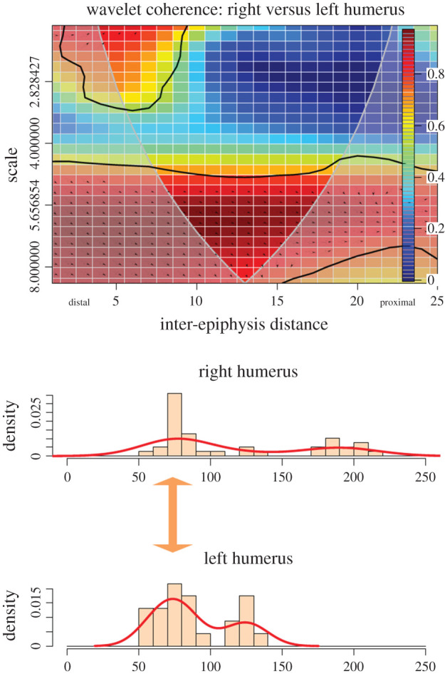
Bivariate wavelet coherence plot showing the correlation of cut mark damage on the proximal, midshaft and distal sections of left and right humeri of the experimental butchery dataset. Arrows indicate that in the high-correlation areas, both series are in phase (i.e. they covary together in the same direction (right)). The thick black line designates the 5% significance level against red noise and the cone of influence. The thick arrow in between histograms indicates locus of high correlation clustering between both series.

Femora show a similarly clear pattern. Isolated or scattered cut marks tend to show the same non-specific locus distribution in both series, as shown by left and right femora showing correlation in the high scale (i.e. low-frequency) distribution of marks along the shaft. Despite the lack of discrete locus correlation, there seems to be a clear coincidence in both series in that cut marks are clustered preferentially on the proximal shaft compared to the distal one, as shown by the spatial correlation area (figure 3). As was the case with humeri, femora display a locus-specific correlation in intensity (i.e. clustering) on the distal metadiaphysis and the proximal epiphysis and metadiaphysis (figure 3). Some marks are, however, more scattered and this implies that there are fewer butchery constraints in filleting through femoral flesh than humeral flesh.

Figure 3.

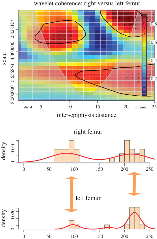
Bivariate wavelet coherence plot showing the correlation of cut mark damage on the proximal, midshaft and distal sections of left and right femora of the experimental butchery dataset. Arrows indicate that in these two high-correlation areas, both series are in phase (i.e. they covary together in the same direction) in some areas, but in lag (they covary in different directions) in the uppermost right area. The thick black line designates the 5% significance level against red noise and the cone of influence. The thick arrows in between histograms indicate loci of high correlation clustering between both series.

For the radius-ulna, both left and right sides show at least three locus-specific clustering spots. One is at the ulna and proximal epiphysis, another is at the proximal radial metadiaphysis and the last, with far less intensity, is at the distal radial metadiaphysis (figure 4). Cut marks occurring scattered along the midshaft are random and show no correspondence between sides.

Figure 4.

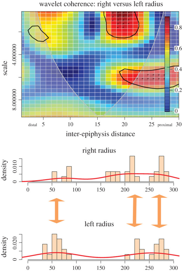
Bivariate wavelet coherence plot showing the correlation of cut mark damage on the proximal, midshaft and distal sections of left and right radius-ulna of the experimental butchery dataset. Arrows indicate that in one high-correlation area, both series are in phase (i.e. they covary together in the same right direction) and in the other they are in lag (left direction). The thick black line designates the 5% significance level against red noise and the cone of influence. The thick arrows in between histograms indicate loci of the high correlation between both series.

WCA also shows that the tibia bears some redundant clustering on the proximal metadiaphysis and more intensively on the distal metadiaphysis (figure 5). There is a wider occurrence of randomness than in other elements, especially when marks occur in low numbers or are scattered. Despite this, when looking at clusters, there is a trend of clusters occurring (in variable intensity) on exactly the same loci (figure 5). As a matter of fact, when observing cut mark distribution between both series, it can be seen that the tibia displays the closest overlap in the coordinate distribution of cut marks, with very few exceeding the 95% confidence ellipses of each overlapping side (figure 5).

Figure 5.

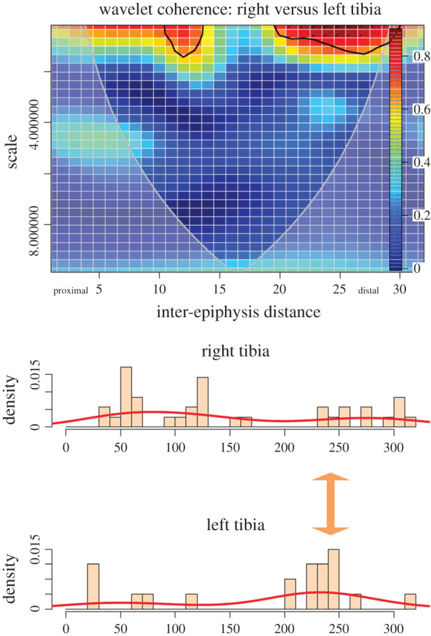
Bivariate wavelet coherence plot showing the correlation of cut mark damage on the proximal, midshaft and distal sections of left and right tibiae of the experimental butchery dataset. Arrows indicate that in one high-correlation area, both series are in lag (i.e. they covary together in different directions). The thick black line designates the 5% significance level against red noise and the cone of influence. The thick arrow in between histograms indicates the locus of high correlation clustering between both series.

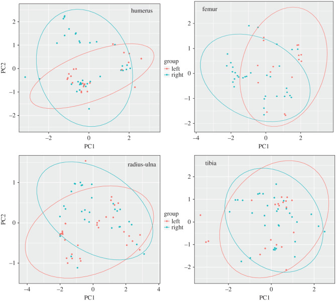
Looking at the raw coordinate distribution of cut marks on the four long bones, the intermediate bones (radius-ulna and tibia) exhibit the closest overlap of most of the documented cut marks between both sides, implying a strong patterning (figure 6). Cut marks occurring outside the overlapping areas of both left and right sides in figure 6 are the ones resulting from randomness. Those documented inside the overlapping ellipses correspond to patterning. As can be seen in figure 6, most cut marks in all elements are patterned. It is only on upper limb bones (humeri, femora) that more marks occur to be random. This is also documented when the confidence ellipses are made around the mean values of each group instead of all points in each group (electronic supplementary material, figure S1).

Figure 6.

Principal component analysis of the raw coordinates (XYZ) of cut marks found on each element of the experimental butchery dataset. A 95% confidence ellipse per group is displayed.

3.2. Sonai Rockshelter dataset: comparison to experimental data

In the Sonai Rockshelter ethnoarchaeological assemblage, not all the long bones and their portions are preserved in the same proportion, reducing comparability to the complete experimental datasets. However, despite the underrepresentation of certain bone portions, the comparison is pertinent to document whether clustering trends documented experimentally also exist in the preserved portions of the ethnoarchaeological assemblage. The bias is limited since the bone portions most prone to underrepresentation at Sonai are mainly epiphyses.

Humeri are cutmarked in similar proportions to those documented experimentally (figure 7). The two most intense clusters are documented on exactly the same locations on both left and right sides. The correlation in scattered marks along the shaft (high scale, low intensity) is moderate, but the one with the highest intensity displays high correlation and concentrates on the distal shaft. The pattern for humeri documented in the Sonai assemblage is virtually the same as in the experiments.

Figure 7.

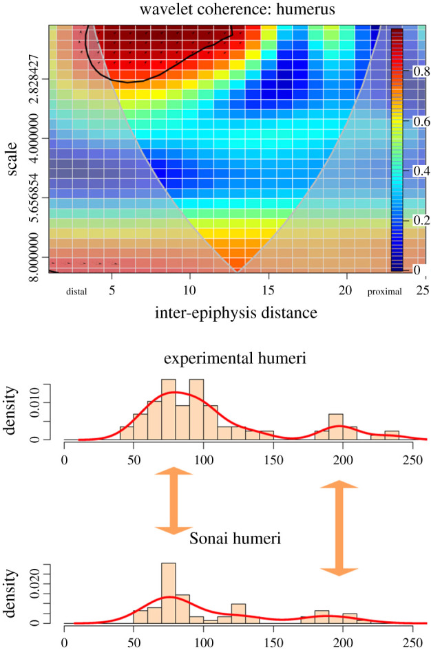
Bivariate wavelet coherence plot showing the correlation of cut mark damage on the proximal, midshaft and distal sections of the humeri of the Sonai ethnoarchaeological dataset and the experimental dataset. Arrows indicate that in one of these two high-correlation areas, both series are in phase (i.e. they covary together in the same right direction). The thick black line designates the 5% significance level against red noise and the cone of influence. The thick arrows in between histograms indicate loci of the high correlation between both series.

The femora show taphonomic biases, since there is a paucity of distal shaft specimens relative to the proximal shaft. The frequency of cut marks longitudinally is, therefore, lower on the distal shaft than documented in the experimental sample. Despite this, wavelet coherence analysis identifies a strong correlation in clustering in the preserved distal shaft (i.e. low scale in figure 8). The correlation identified in the non-biased femoral sample from Sonai is very high with the experimental sample precisely in the same loci as where the bilateral correlation of the experimental sample was documented (figure 8). Both low-density mark areas and high-density mark areas are highly correlated, indicating that in the proximal femoral shaft and epiphysis, scattered and clustered marks tend to occur in the same loci.

Figure 8.

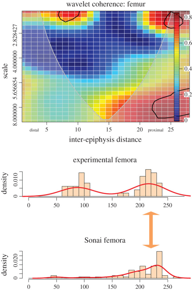
Bivariate wavelet coherence plot showing the correlation of cut mark damage on the proximal, midshaft and distal sections of the femora of the Sonai ethnoarchaeological dataset and the experimental dataset. The thick black line designates the 5% significance level against red noise and the cone of influence. The thick arrow in between histograms indicates the locus of the high correlation between both series.

The radius-ulna shows some differences with the upper limb bones. The Sonai radii-ulnae are less cutmarked than the experimental sample and the correlation between both sides is found in only two loci, instead of three. One is situated on the proximal shaft, where the intensity is low (i.e. high scale). The high clustering documented on the proximal metadiaphysis and epiphysis in the experimental sample is not observed at Sonai. However, the occurrence of isolated marks or marks in low densities is similar in both series. The wavelet coherence test also succeeds at detecting the high correlation of marks on the distal metadiaphysis, despite the smaller sample from Sonai due to taphonomic bias (figure 9).

Figure 9.

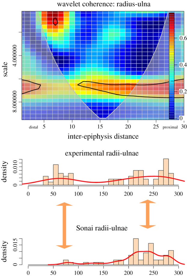
Bivariate wavelet coherence plot showing the correlation of cut mark damage on the proximal, midshaft and distal sections of the radii-ulnae of the Sonai ethnoarchaeological dataset and the experimental dataset. The thick black line designates the 5% significance level against red noise and the cone of influence. The thick arrows in between histograms indicate loci of the high correlation between both series.

Finally, in the tibia, there is a correlation between both left and right sides in both areas that were patterned in the experimental sample alone: the proximal metadiaphysis (moderately) and the distal shaft. There is a higher variability in the intensity of cut marks on the proximal shaft than in the distal shaft. Although the wavelet coherence analysis also shows a strong correlation in low-density scatters of marks along the shaft (i.e. high scale), this reflects that cutmarking the shaft longitudinally without any specific locus is something that both series have in common (figure 10). Interestingly, a new clustering locus on the midshaft emerges when comparing both samples (figure 10).

Figure 10.

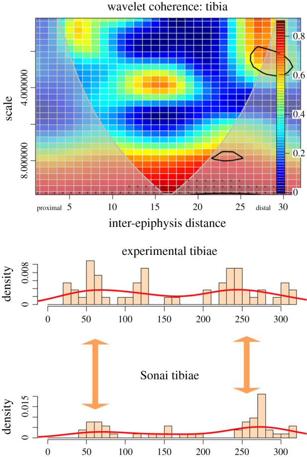
Bivariate wavelet coherence plot showing the correlation of cut mark damage on the proximal, midshaft and distal sections of the tibiae of the Sonai ethnoarchaeological dataset and the experimental dataset. Arrows indicate that in these two high-correlation areas, both series are in phase (i.e. they covary together in the same direction). The thick black line designates the 5% significance level against red noise and the cone of influence. The thick arrows in between histograms indicate loci of the high correlation between both series.

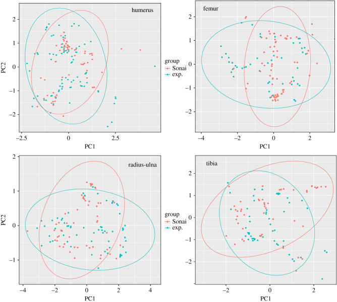
These interpretations are further supported when observing the PCA of the distribution of the raw coordinates of the cut mark set for both series (figure 11). Most cut marks occupy overlapping spaces between both 95% confidence ellipses, with fewer being the result of stochastic marking during butchery. The experimental sample shows more marks outside the overlapping spaces indicating more randomness in their production, as would be expected in novice butchers. There is a good match in patterns documented in humeri and radii-ulnae, with more marks due to randomness in femora and tibiae. However, when the ellipses are made around each category's values the patterning is tight even in femora and tibiae (electronic supplementary material, figure S2).

Figure 11.

Principal component analysis of the raw coordinates (XYZ) of cut marks found on each element of the experimental butchery dataset and the Sonai assemblage. A 95% confidence ellipse per group is displayed.

In summary, the bulk of cut mark intensity processes, regardless of their actual degree, seem to be spatially discrete and clustered, following patterning in both series.

3.3. Comparison of the experimental, ethnoarchaeological and the Tarangire felid–hominin long series

A comparison of the long series of all meat-bearing bones between the experimental butchery assemblage and the Sonai ethnoarchaeological assemblage shows that both series are strongly correlated in the distribution of clustering of high numbers of marks on the distal shafts and mid-shafts of humeri and femora. They also show that they are in phase (i.e. they vary with the same proportional intensity on similar or the same locations) when marks on upper limb bones are moderate in number and even when they occur scattered. Both series are also highly correlated and in phase with moderate clustering of cut marks on the proximal radius-ulna shafts. Correlation of clustering of cut marks on the distal tibia seems also documented on both series (figure 12).

Figure 12.

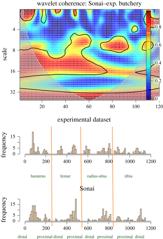
Bivariate wavelet coherence plot showing the correlation of cut mark damage on the long series (humeri, femora, radii-ulnae and tibiae) of the Sonai ethnoarchaeological assemblage and the experimental dataset. Arrows indicate that in the four high-correlation areas, both series are in phase (i.e. they covary together in the same direction). The thick contour line designates the 5% significance level against red noise and the cone of influence.

Given the adequacy of either series for reproducing butchery of fully fleshed carcasses, we selected only one of them (the Sonai ethnoarchaeological assemblage) for comparison with the long series resulting from defleshing the 10 carcasses obtained at the Tarangire lion kills [35]. There are coincidences and divergences with the patterns documented with the butchery of fully fleshed carcasses (figure 13). Cut marks on distal shafts and mid-shafts of humeri seem to covary in both series (i.e. both assemblages). Such covariation is substantially less marked in the proximal radii-ulnae and on tibiae. Low-frequency clustering of cut marks is also correlated in the radius-ulna. With the exception of the proximal radius-ulna and distal half of the humeral shaft, the correlation between both series is weaker than between the two series representing full butchery of carcasses (experimental and Sonai). This divergence between the Sonai and Tarangire datasets is mostly expressed in the substantially lower intensity of cutmarking in the latter, but despite this, there is a clear correspondence in the locations where the less modified Tarangire carcasses display cut marks and those of the Sonai assemblage. In both cases, most clustering and occurrence of cut marks tends to occur on the same loci. The most drastic divergence is documented in the femora, which exhibit fewer and more randomly scattered cut marks in the Tarangire carcasses, probably because femora were almost completely defleshed by lions. Something similar occurs on humeri, where although the few cut marks documented on the Tarangire carcasses correspond to the clustering areas of the Sonai assemblage, those are more extensive in the Sonai dataset.

Figure 13.

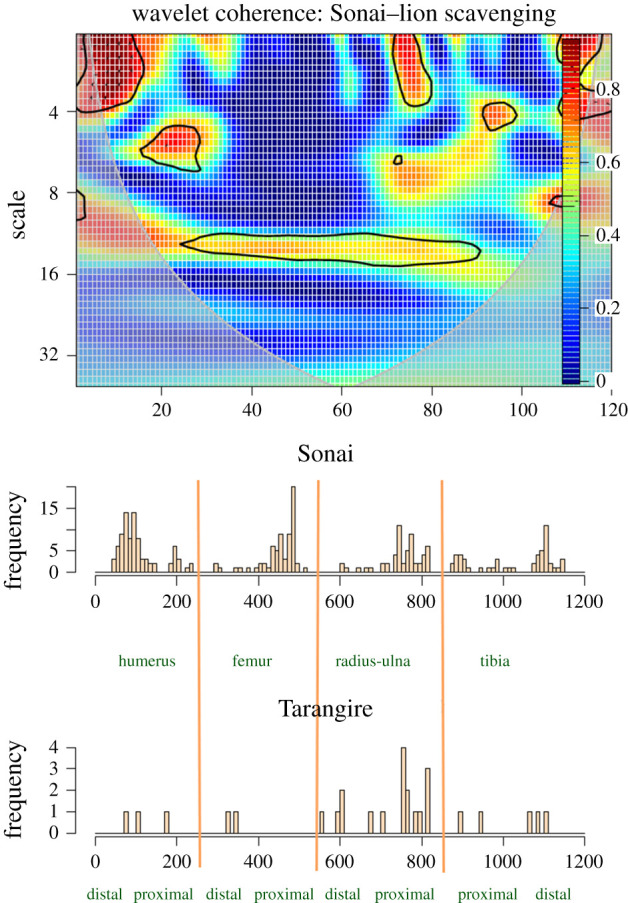
Bivariate wavelet coherence plot showing the correlation of cut mark damage on the long series (humeri, femora, radii-ulnae and tibiae) of the Sonai ethnoarchaeological assemblage and the Tarangire lion dataset. Arrows indicate that in the four high-correlation areas, both series are in phase (i.e. they covary together in the same direction). The thick contour line designates the 5% significance level against red noise and the cone of influence.

Overall, these results show that the more intensive defleshing of upper limb bones by lions leaves fewer flesh scraps and, as a result, fewer opportunities for generating cut mark clustering, resulting in only isolated occurrences of cut marks on these elements compared to the butchery of fully fleshed carcasses. This is also documented on the intermediate limb bones, but less so given the higher variability of flesh survival in these elements. The overlap in zones of cutmarking between both series (i.e. Sonai and Tarangire) indicates profound constrictions in where marks occur due to muscle insertion and butchery ergonomics. The differences between both series also shows that the higher and more widespread occurrence of cut marks on the fully fleshed butchery experiments also shows areas on each element where cut marks may not occur on the Tarangire sample because they do not contain any flesh. Indirectly, these three-dimensional spatial documentation of cut marks shows that the division of hot and cold (areas without or with the survival of flesh scraps or muscle insertions after felid consumption) zones is justified [24].

The different wavelet coherence graphs show that patterned differences can be obtained when comparing butchery models using complete carcasses and when using largely defleshed carcasses from felid kills.

3.4. Classification of multiple patterns through the comparison of primary and secondary access

In order to compare scenarios of primary access (butchery of fleshed carcasses) to those of secondary access (butchery of defleshed carcasses), all the similarities and differences outlined in the previous section were computed through a hierarchical clustering test. The phylogenetic graph best enables us to graphically show differences in variance among multiple models. Figure 14 shows that the two samples involving butchery of complete carcasses (experimental and Sonai) cluster in proximity to each other, whereas the Tarangire sample of defleshed carcasses clusters away from them. This approach shows that differences among models can be used to efficiently cluster them according to how similar or dissimilar they are. This is only possible because cutmarking follows intrinsic patterning.

Figure 14.

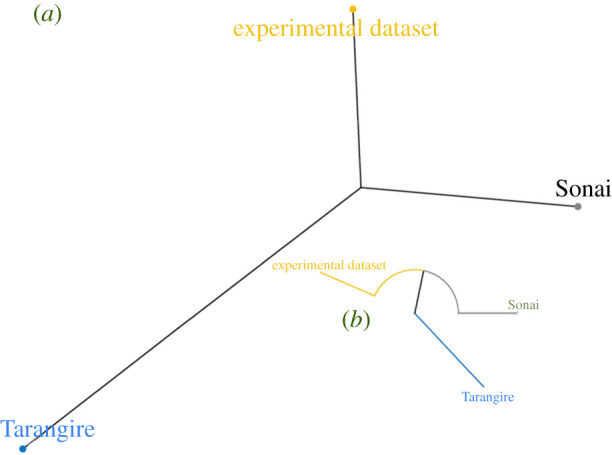
Phylogenetic (a) and circular (b) dendrograms showing the distances of the wavelet spectra of the cutmarking patterns from the three series analysed: experimental butchery, Sonai ethnoarchaeological assemblage and the Tarangire lion carcasses.

4. Discussion

Inferences of butchery patterns have traditionally been made using comparative frameworks. However, this has led to divergent interpretations according to which analogical framework is used. For instance, something as simple as inferring butchery behaviour (i.e. filleting or dismembering) using cut marks on proximal and distal ends of long bones may lead to different interpretations depending on whether one uses Binford's [41], Nilssen's [30], Galán & Domínguez-Rodrigo's [10] or Soulier & Costamagno's [12] ethnoarchaeological and experimental analogues. This is because each of these frameworks has been derived through multiple different variables in each case, and in some cases, there is also a lack of control over cause–effect (more specifically, effector–trace) relationships [42]. This creates inferential uncertainty.

There is undoubtedly a random component in cut mark frequencies and anatomical distribution, but as the present study shows, this randomness overlies a highly patterned occurrence of cut mark clusterings. There are preferential areas on long bones where cut marks concentrate, probably because of an interplay of variables, among which muscle, tendon and ligament insertions, and the ergonomics of butchery, are some of the most relevant.

Our first research question asked whether there was statistically significant patterning in the distribution of cut marks on all meat-bearing long bones produced during butchery. Our results show that, indeed, these patterns do exist and are statistically significant. The second question asked whether these patterns were restricted to specific bones due to the influence of specific muscle locations and/or the ergonomics of butchery. Our results show that these patterns are not restricted to specific bones, but rather are found on all five meat-bearing long bones analysed; however, such patterns are stronger for certain elements, like radius-ulna and tibia. Our third question asked whether different types of human access to carcasses (primary versus secondary) could be determined through behaviour-specific cutmark patterns. Here, the wavelet method showed that butchery of fully fleshed carcasses (experimental and Sonai samples) and scavenged carcasses (Tarangire sample) can be efficiently differentiated. This brings us to the fourth question, whether butchery patterns can be objectively classified and compared across assemblages. Our results show that even similar butchery behaviours under different conditions can generate enough (even when subtle) dissimilarity distances to enable the method to identify them, cluster or separate them, and classify them in an objective way. This helps to move taphonomic analysis beyond descriptive methods and shows a real ability to mathematically separate assemblages.

The butchery patterning documented here is so defined that clustering of cutmarks occurs on most of the same bone portions and locations (with clearly different intensities) on fleshed and largely defleshed carcasses, on small and larger carcasses, on butchery done with metal or stone tools, and with experienced or novice butchers. It is the set of variations documented in the reported butchery patterns that enables the separation and identification of each of them. If cut marks are still considered to be accidents, they must be seen under the new light of accidents waiting to happen, on specific bone locations and under certain behaviours.

5. Conclusion

Butchery patterns in the form of cut mark clustering and occurrence are intrinsic to the butchery process. The highly variable intensity of cut marks on faunal assemblages and the occurrence of isolated or scattered marks may have a strong stochastic component, but clustering seems to be highly predictable as shown by the existence of patterning. Specific patterning of cut marks has been documented for each of the five meat-bearing bones. Differences among experimental and ethnoarchaeological samples reflecting butchery of complete carcasses have been shown. Differences with the butchery of scavenged carcasses from lion kills also reflect patterning. The methods implemented in the present study allow the detection of the dissimilarities among assemblage and create matritial distances that allow their objective classification. Our analytical approach moves beyond description and classification based on simple quantification. The use of exact three-dimensional information about BSM locations, through Ikhnos software, supposes an advantage for the efficient spatial analysis of BSM in general, and specifically of cut marks in the present study. We emphasize the use of strictly analytical methods for reconstructing behaviours from the anatomical distribution and intensity of cut marks in archaeofaunal assemblages. One of the potential future outcomes of this approach could be the detailed analysis of butchery patterning among groups caused by culturally distinctive culinary practices.

Data accessibility

This article has no additional data.

Authors' contributions

M.P.-M., M.E.P., A.O.G., E.B. collected data. M.P.-M., M.E.P., A.O.G., M.D.-R. conducted analysis. R.M., D.G.-A., M.A.M.-G. created the software.

Competing interests

We declare we have no competing interests.

Funding

We thank the Spanish Ministry of Education and Science for funding this research (HAR2017-82463-C4-1-P). Research at Sonai Rockshelter was funded by grants to M.E.P. from the National Science Foundation (Doctoral Dissertation Improvement Grant, no. 0620262) and Wenner-Gren Foundation (Dissertation Fieldwork Grant, no. 7489).

References

- 1.Lyman RL 1987. Archaeofaunas and butchery studies: a taphonomic perspective. Adv. Archaeol. Method Theory 10, 249–337. ( 10.1016/B978-0-12-003110-8.50008-6) [DOI] [Google Scholar]
- 2.Lyman RL 1995. A study of variation in the prehistoric butchery of large artiodactyls. In Ancient peoples and landscapes (ed. Johnson E), pp. 233–253. Lubbock, TX: Museum of Texas Tech University. [Google Scholar]
- 3.Lyman RL 1994. Vertebrate taphonomy. Cambridge, UK: Cambridge University Press. [Google Scholar]
- 4.Walker PL, Long JC. 1977. An experimental study of the morphological characteristics of tool marks. Am. Antiq. 42, 605–616. ( 10.2307/278934) [DOI] [Google Scholar]
- 5.Greenfield HJ 1999. The origins of metallurgy: distinguishing stone from metal cut-marks on bones from archaeological sites. J. Archaeol. Sci. 26, 797–808. ( 10.1006/jasc.1998.0348) [DOI] [Google Scholar]
- 6.Greenfield HJ 2002. Distinguishing metal (steel and low-tin bronze) from stone (flint and obsidian) tool cut marks on bone: an experimental approach. Exp. Archaeol. Replicating Past Objects Behav. Process. 1035, 35. [Google Scholar]
- 7.Bello SM, Parfitt SA, Stringer C. 2009. Quantitative micromorphological analyses of cut marks produced by ancient and modern handaxes. J. Archaeol. Sci. 36, 1869–1880. ( 10.1016/j.jas.2009.04.014) [DOI] [Google Scholar]
- 8.Egeland CP 2012. The use of bone surface modifications to model hominid lifeways during the Oldowan. In Stone tools and fossil bones: debates in the archaeology of human origins (ed. Domínguez-Rodrigo M), pp. 80–114. Cambridge, UK: Cambridge University Press. [Google Scholar]
- 9.Machin AJ, Hosfield R, Mithen SJ. 2016. Testing the functional utility of handaxe symmetry: fallow deer butchery with replica handaxes. Lithics J. Lithic Stud. Soc. 26, 23–37. [Google Scholar]
- 10.Galán AB, Domínguez-Rodrigo M. 2013. An experimental study of the anatomical distribution of cut marks created by filleting and disarticulation on long bone ends. Archaeometry 55, 1132–1149. ( 10.1111/j.1475-4754.2012.00730.x) [DOI] [Google Scholar]
- 11.Galán AB, Domínguez-Rodrigo M. 2014. Testing the efficiency of simple flakes, retouched flakes and small handaxes during butchery. Archaeometry 56, 1054–1074. ( 10.1111/arcm.12064) [DOI] [Google Scholar]
- 12.Soulier M-C, Costamagno S. 2017. Let the cutmarks speak! Experimental butchery to reconstruct carcass processing. J. Archaeol. Sci. Rep. 11, 782–802. ( 10.1016/j.jasrep.2016.12.033) [DOI] [Google Scholar]
- 13.Costamagno S, Soulier M-C, Val A, Chong S. 2019. The reference collection of cutmarks. Palethnologie ( 10.4000/palethnologie.4089) [DOI] [Google Scholar]
- 14.Selvaggio MM 1994. Carnivore tooth marks and stone tool butchery marks on scavenged bones: archaeological implications. J. Hum. Evol. 27, 215–228. ( 10.1006/jhev.1994.1043) [DOI] [Google Scholar]
- 15.Blumenschine RJ 1995. Percussion marks, tooth marks, and experimental determinations of the timing of hominid and carnivore access to long bones at FLK Zinjanthropus, Olduvai Gorge, Tanzania. J. Hum. Evol. 29, 21–51. ( 10.1006/jhev.1995.1046) [DOI] [Google Scholar]
- 16.Capaldo SD 1998. Simulating the formation of dual-patterned archaeofaunal assemblages with experimental control samples. J. Archaeol. Sci. 25, 311–330. ( 10.1006/jasc.1997.0238) [DOI] [Google Scholar]
- 17.López-Cisneros P, Yravedra J, Álvarez-Alonso D, Linares-Matás G. 2019. The exploitation of hunted resources during the Magdalenian in the Cantabrian region. Systematization of butchery processes at Coímbre cave (Asturias, Spain). Quat. Int. 506, 46–58. ( 10.1016/j.quaint.2018.05.035) [DOI] [Google Scholar]
- 18.Parkinson JA, Plummer T, Hartstone-Rose A. 2015. Characterizing felid tooth marking and gross bone damage patterns using GIS image analysis: an experimental feeding study with large felids. J. Hum. Evol. 80, 114–134. ( 10.1016/j.jhevol.2014.10.011) [DOI] [PubMed] [Google Scholar]
- 19.Pobiner B, Dumouchel L, Parkinson J. 2020. A new semi-quantitative method for coding carnivore chewing damage with an application to modern African lion-damaged bones. Palaios 35, 302–315. ( 10.2110/palo.2019.095) [DOI] [Google Scholar]
- 20.Parkinson JA, Plummer TW, Bose R. 2014. A GIS-based approach to documenting large canid damage to bones. Palaeogeogr. Palaeoclimatol. Palaeoecol. 409, 57–71. ( 10.1016/j.palaeo.2014.04.019) [DOI] [Google Scholar]
- 21.Yravedra J, Maté-González MÁ, Courtenay LA, González-Aguilera D, Fernández MF. 2019. The use of canid tooth marks on bone for the identification of livestock predation. Sci. Rep. 9, 16301 ( 10.1038/s41598-019-52807-0) [DOI] [PMC free article] [PubMed] [Google Scholar]
- 22.Rodrigo MD, Pickering TR. 2010. A multivariate approach for discriminating bone accumulations created by spotted hyenas and leopards: harnessing actualistic data from East and Southern Africa. J. Taphon. 8, 155–179. [Google Scholar]
- 23.Domínguez-Rodrigo M 1997. Testing meat-eating in early hominids: an analysis of butchery marks on defleshed carcases. Hum. Evol. 12, 169–182. ( 10.1007/BF02438066) [DOI] [Google Scholar]
- 24.Domínguez-Rodrigo M, et al. Submitted. A 3D taphonomic model of long bone modification by lions in medium-sized ungulate carcasses. [DOI] [PMC free article] [PubMed]
- 25.Domínguez-Rodrigo M, Bunn HT, Yravedra J. 2014. A critical re-evaluation of bone surface modification models for inferring fossil hominin and carnivore interactions through a multivariate approach: application to the FLK Zinj archaeofaunal assemblage (Olduvai Gorge, Tanzania). Quat. Int . 322–323, 32–43. ( 10.1016/j.quaint.2013.09.042) [DOI] [Google Scholar]
- 26.Blasco R, et al. 2013. Learning by heart: cultural patterns in the faunal processing sequence during the middle pleistocene. PLoS ONE 8, e55863 ( 10.1371/journal.pone.0055863) [DOI] [PMC free article] [PubMed] [Google Scholar]
- 27.Blasco R, Domínguez-Rodrigo M, Arilla M, Camarós E, Rosell J. 2014. Breaking bones to obtain marrow: a comparative study between percussion by batting bone on an anvil and hammerstone percussion: breaking bones to obtain marrow. Archaeometry 56, 1085–1104. ( 10.1111/arcm.12084) [DOI] [Google Scholar]
- 28.Vettese D, Daujeard C, Blasco R, Borel A, Caceres I, Moncel MH. 2017. Neandertal long bone breakage process: standardized or random patterns? The example of Abri du Maras (Southeastern France, MIS 3). J. Archaeol. Sci. Rep. 13, 151–163. ( 10.1016/j.jasrep.2017.03.029) [DOI] [Google Scholar]
- 29.Stavrova T, Borel A, Daujeard C, Vettese D. 2019. A GIS based approach to long bone breakage patterns derived from marrow extraction. PLoS ONE 14, e0216733 ( 10.1371/journal.pone.0216733) [DOI] [PMC free article] [PubMed] [Google Scholar]
- 30.Nilssen PJ 2000. An actualistic butchery study in South Africa and its implications for reconstructing hominid strategies of carcass acquisition and butchery in the upper pleistocene and plio-pleistocene. Cape Town, South Africa: University of Cape Town. [Google Scholar]
- 31.Barba R 2008. Nueva aproximación tafonómica al estudio de las marcas de corte para el debate de caza y carroñeo en yacimientos africanos: aplicación al FLK Zinj (Olduvai, Tanzania)/A new taphonomic approach to the study of cut marks for the hunting-and-scavenging debate in Early African sites and its application to the FLK Zinj (Olduvai Gorge, Tanzania). Complutum 19, 9–24. [Google Scholar]
- 32.Domínguez-Rodrigo M, Barba R. 2005. A study of cut marks on small-sized carcasses and its application to the study of cut-marked bones from small mammals at the FLK Zinj site. J. Taphon. 3, 121–134. [Google Scholar]
- 33.Prendergast ME 2008. Forager variability and transitions to food production in secondary settings: Kansyore and Pastoral Neolithic economies in East Africa. PhD dissertation, Anthropology Department, Harvard University, Cambridge, MA. [Google Scholar]
- 34.Marlowe F 2010. The Hadza: hunter-gatherers of Tanzania. Oakland, CA: University of California Press. [Google Scholar]
- 35.Gidna AO, Kisui B, Mabulla A, Musiba C, Domínguez-Rodrigo M. 2014. An ecological neo-taphonomic study of carcass consumption by lions in Tarangire National Park (Tanzania) and its relevance for human evolutionary biology. Quat. Int . 322–323, 167–180. ( 10.1016/j.quaint.2013.08.059) [DOI] [Google Scholar]
- 36.Grinsted A, Moore JC, Jevrejeva S. 2004. Application of the cross wavelet transform and wavelet coherence to geophysical time series. Nonlinear Process. Geophys. 11, 561–566. ( 10.5194/npg-11-561-2004) [DOI] [Google Scholar]
- 37.Nason G 2008. Wavelet methods in statistics with R. Berlin, Germany: Springer Science & Business Media. [Google Scholar]
- 38.Torrence C, Compo GP. 1998. A practical guide to wavelet analysis. Bull. Am. Meteorol. Soc. 79, 61–78. () [DOI] [Google Scholar]
- 39.Chavez M, Cazelles B. 2019. Detecting dynamic spatial correlation patterns with generalized wavelet coherence and non-stationary surrogate data. Sci. Rep. 9, 7389 ( 10.1038/s41598-019-43571-2) [DOI] [PMC free article] [PubMed] [Google Scholar]
- 40.Baddeley A, Rubak E, Turner R. 2015. Spatial point patterns: methodology and applications with R. Boca Raton, FL: CRC Press. [Google Scholar]
- 41.Binford LR 1981. Bones: ancient men and modern myths. New York, NY: Academic Press. [Google Scholar]
- 42.Gifford-Gonzalez D 1991. Bones are not enough: analogues, knowledge, and interpretive strategies in zooarchaeology. J. Anthropol. Archaeol. 10, 215–254. ( 10.1016/0278-4165(91)90014-O) [DOI] [Google Scholar]
Associated Data
This section collects any data citations, data availability statements, or supplementary materials included in this article.
Supplementary Materials
Data Availability Statement