Variability and sampling of lead (Pb) in drinking water: Assessing potential human exposure depends on the sampling protocol

Abstract

Lead (Pb) in drinking water has re-emerged as a modern public health threat which can vary widely in space and in time (i.e., between homes, within homes and even at the same tap over time). Spatial and temporal water Pb variability in buildings is the combined result of water chemistry, hydraulics, Pb plumbing materials and water use patterns. This makes it challenging to obtain meaningful water Pb data with which to estimate potential exposure to residents. The objectives of this review paper are to describe the root causes of intrinsic Pb variability in drinking water, which in turn impacts the numerous existing water sampling protocols for Pb. Such knowledge can assist the public health community, the drinking water industry, and other interested groups to interpret/compare existing drinking water Pb data, develop appropriate sampling protocols to answer specific questions relating to Pb in water, and understand potential exposure to Pb-contaminated water. Overall, review of the literature indicated that drinking water sampling for Pb assessment can serve many purposes. Regulatory compliance sampling protocols are useful in assessing community-wide compliance with a water Pb regulatory standard by typically employing practical single samples. More complex multi-sample protocols are useful for comprehensive Pb plumbing source determination (e.g., Pb service line, Pb brass faucet, Pb solder joint) or Pb form identification (i.e., particulate Pb release) in buildings. Exposure assessment sampling can employ cumulative water samples that directly capture an approximate average water Pb concentration over a prolonged period of normal household water use. Exposure assessment may conceivably also employ frequent random single samples, but this approach warrants further investigation. Each protocol has a specific use answering one or more questions relevant to Pb in water. In order to establish statistical correlations to blood Pb measurements or to predict blood Pb levels from existing datasets, the suitability of available drinking water Pb datasets in representing water Pb exposure needs to be understood and the uncertainties need to be characterized.

1. Introduction

More than a decade after the Washington DC water lead (Pb) crisis (Edwards et al., 2009; Edwards, 2014), new correlations between elevated water Pb and elevated childhood blood Pb in Flint, MI (Hanna-Attisha et al. 2016) reinvigorated public interest on drinking water as a Pb exposure source. This motivated new exposure and blood Pb modeling predictions based on available and hypothetical Pb datasets (Stanek et al., 2020; Zartarian et al., 2017).

If Pb contamination of drinking water was consistently uniform across and within residences and buildings, then any sampling protocol would be capable of capturing that fixed Pb concentration. It could then be extrapolated to potential ingestion exposure with knowledge of the amount of water consumed. However, Pb in drinking water can vary widely in space and in time (i.e., between homes, within homes and even at the same tap over time), as the combined result of water chemistry, hydraulics, Pb plumbing sources and water consumption patterns among individuals (Fig. 1). This makes it challenging to obtain meaningful water Pb data with which to estimate potential exposure to residents and may have at least partly contributed to the perception that water Pb is a small contributor to blood Pb (Triantafyllidou and Edwards 2012).

Fig. 1.

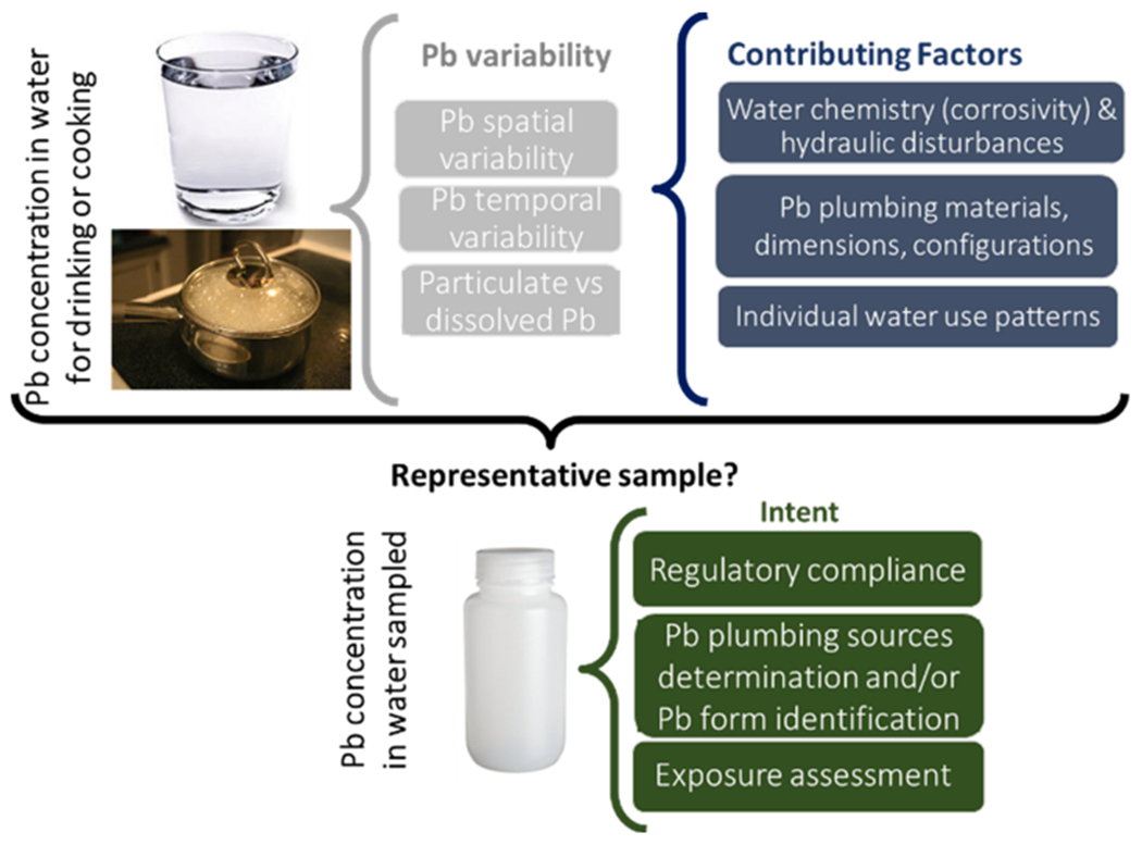
General factors contributing to lead (Pb) variability in the drinking water that is consumed or sampled.

Historically, studies used Pb datasets obtained by a variety of sampling protocols to assess the contribution of water Pb to the body’s total Pb burden (Table 1). However, if the ultimate goal is drinking water Pb exposure characterization, defined as the quantitative assessment of the ingested Pb which combines Pb concentration and volume of water consumed (U.S. EPA 2019), then collected samples should capture the spatial/temporal variability of water Pb that consumers cumulatively ingest during their water use patterns. Understanding the root causes of intrinsic Pb variability in water and the numerous existing water sampling protocols for Pb will assist the public health community, the drinking water industry and other interested groups to:

• interpret/compare existing drinking water Pb data obtained by various sampling protocols,

• develop appropriate sampling protocols to answer specific questions relating to Pb in water, and

• specifically evaluate the potential exposure to Pb-contaminated water and its potential error bounds

Table 1.

Illustrative water sampling protocols in studies that attempted to assess the contribution of water Pb to total Pb exposure. The list is not exhaustive.

Study (Chronological Order)	Water Sampling Protocol at Each Building (Home or School)
Beattie et al. 1972	First-draw sample after overnight stagnation
Elwood et al. 1976	Two samples of 1–2 pints (0.5–1 L) from kitchen tap: • Morning sample with first run-off in the day, followed by • Evening sample taken later in the day
Greathouse et al. 1976, Worth et al. 1981	Four samples: • Standing sample from cold water tap after turning it on and rinsing out the sample container • Running sample from cold water tap after 4-min flush • Composite sample by resident in 1-gallon sample bottle filled with 1 quart of water at each meal for 1 day • Early morning sample by resident in 1-quart sample bottle filled in early morning at the time the resident felt a temperature change in the water (i.e. from warm to cold)
Moore et al. 1979	Two samples: • One 250-mL first flush in the morning from the cold tap used for food preparation, followed by • At least 5-min flush
Thomas et al. 1979	Three samples (1.2 L) from the cold kitchen tap on three occasions at 2-week intervals: • Daytime (first water out of the tap at the time of visit) • Running (after running the tap moderately for 5-min after the daytime sample) • First flush (first water out of the tap in the morning, collected by residents)
Sherlock et al. 1982	Four 200 mL samples from kettles, taken at different times on different days during a designated week
Pocock et al. 1983	Three 1-L samples: • First-draw from kitchen tap in the morning • Random daytime later in the day • Flushed sample after an estimated 10 pipe volumes of water had been flushed
Lacey et al. 1985	Four samples (variable volume): • Composite kettle sample over a week, comprised of individual 200 mL drawn from kettle daily to make baby’s first feed of the day, and then poured into a 1.5 L polythene bottle marked at 7 levels • 1-L first draw sample after overnight stagnation • 1-L random daytime sample • 1-L from hot tap, for households with suspiciously high or inconsistent values
Sherlock and Quinn 1986	• Random daytime sample and sequential profile samples by water authority • Single sample of 200 mL kettle water; composite sample of kettle water each day, and 1-L first-draw sample by residents
Raab et al. 1987	One 30-min stagnation sample from kitchen cold water (unspecified volume)
Laxen et al. 1987	One kitchen cold water sample after a 30-min stagnation and a 5-min flush
Davies et al. 1990	7-day composite sample
Maes et al. 1991	One 1-L sample from an exterior house faucet, without regard to time of day, after at least 2-min flush and observing stable water temperature by touch
Raab et al. 1993	Two 1-L samples: • 30-min stagnation sample from kitchen cold tap • Flushed sample from kitchen hot tap after reaching stable temperature
Lanphear et al. 1996a	Two 1-L water samples: • First-draw sample, followed by • 1-min flush
Lanphear et al. 1996b	1-min flush sample
Watt et al. 1996	• 30 mL water sample from the household kettle by residents • Repeat kettle water sample and a daytime water sample (1 L sample taken from the drinking water tap with no prior flushing) by research nurse
Watt et al. 2000	• 30 mL water sample from the household kettle by residents • Repeat kettle water sample, a daytime water sample (1-L taken from the drinking water tap with no prior flushing, and a 30-min stagnation (1-L taken after approximately 5 pipe volumes had been flushed and 30-min stagnation was subsequently employed) by research nurse
Fertmann et al. 2004	Three samples (unspecified volumes): • Stagnant sample in morning, followed by 3-min flush sample, and then sample intended for cooking at lunchtime
Sathyanarayana et al., 2006; Triantafyllidou et al., 2014	250-mL samples (obtained from school sampling following EPA’s 3 T’s guidance): • Standing samples after 8–18 h stagnation, followed by running samples after a 30-sec flush in water fountains/faucets
Levallois et al. 2014	Five 1-L tap water samples from cold kitchen tap with the aerator on: • 5-min flush at typical flow rate, followed by four consecutive samples after a 30-min stagnation
Ngueta et al. 2014	Five 1-L samples: • 5-min flush sample, followed by a 30-min stagnation sample after which 4 consecutive samples were collected (Flow rate maintained at 5–7 L/min and tap aerators were intact during sampling)
Etchevers et al., 2015	One 2-L sample after a 30-min stagnation
Safruk et al. 2017	Three 1-L samples: • 5-min flushed sample, followed by • 30-min stagnation sample • Then 2-L of water was wasted, and the fourth liter was collected (water presumably in contact with the service line)
Zartarian et al. 2017	One 1-L first-draw sample from interior tap after at least 6-h stagnation obtained from US water utilities’ compliance monitoring
Deshommes et al., 2018	Sequential profile samples (four to sixteen 1-L samples) after 30-min stagnation
Jarvis et al. 2018	Sub-samples from each drink consumed at home over three days in winter and summer
Riblet et al. 2019	Composite proportional sample (5% side stream of water used for cooking/drinking for 1–2 weeks) compared to RDT, first-draw, 30-min stagnation and 5-min flushed samples
Stanek et al. 2020	Sequential profile samples obtained from US water utilities, EPA offices and other studies

2. Factors affecting Pb variability in drinking water

Early research set the groundwork of Pb variability in drinking water (e.g., Britton and Richards, 1981; Kuch and Wagner, 1983; Schock, 1990; Sheiham and Jackson, 1981; Wagner and Kuch, 1981). Subsequent advances allowed further exploration of the root causes of variability, classified into 3 general categories below.

2.1. Water chemistry and hydraulic changes

A plethora of water chemistry parameters (Box 1) affect how quickly dissolved Pb is released into the water (kinetics), the maximum dissolved Pb concentration reached at equilibrium (plumbosolvency) and the resulting corroded Pb pipe surface composition (corrosion scale chemical and hydraulic durability). Reviews of water chemistry and Pb plumbing corrosion as they affect Pb release can be found elsewhere (AWWARF, 1990; Kim et al., 2011; Lytle and Schock, 2000; Schock et al., 1996; Schock and Lytle, 2011).

Box 1.

Some main drinking water chemistry parameters affecting Pb release. The list is not meant to be exhaustive.

• pH and alkalinity/Dissolved Inorganic Carbon (DIC)

• Oxidant type (e.g., chlorine, chloramine, dissolved oxygen) and concentration

• Oxidation Reduction Potential (ORP)

• Corrosion inhibitor type (e.g., none, orthophosphate, orthophosphate/polyphosphate blend, silica) and concentration

• Chloride and sulfate

• Iron, calcium, manganese, aluminum

• Natural Organic Matter (NOM)

Seasonal fluctuations in incoming water chemistry and temperature may affect Pb corrosion reactions and result in temporal changes to Pb release (Deshommes et al., 2013; Jarvis et al., 2018; Masters et al., 2016a; Ngueta et al., 2014; Schock and Lemieux, 2010). Lead corrosion scales often have multiple layers of varying composition which are controlled by water chemistry. An outermost corrosion scale layer with high Pb solubility or low mechanical durability can be more susceptible to Pb release due to the inherent water chemistry or due to hydraulic changes (Del Toral et al., 2013; Sandvig et al., 2008; Wasserstrom et al., 2017). Water chemistry changes and hydraulic changes can release particulate Pb in a seemingly random fashion, further contributing to variability (Masters et al., 2016b; Schock, 1990; Triantafyllidou and Edwards, 2012). Capturing total Pb release (particulate and dissolved Pb) with standard sampling protocols is challenging, given the unpredictable nature of particulate release (Clark et al., 2014; Triantafyllidou and Edwards, 2012).

2.2. Lead spatial variability in plumbing

Premise plumbing systems are complex pipe networks in buildings that deliver water to drinking water outlets, such as devices intended for consumptive purposes (e.g., drinking water faucets, drinking water fountains, icemakers), and fixtures intended for non-consumptive purposes (e.g., garden faucets, utility sinks, showerheads, toilets, furnace humidifiers, bathroom faucets). Some water outlets may be used for both purposes by design, practicality, or personal behavior. Lead in water may originate from a variety of plumbing sources (Fig. 2), which can differ in type, number, location, diameter and length within and between premise plumbing systems. For simplicity, premise plumbing in this work refers to all building types (e.g., residential homes, residential apartment complexes and non-residential buildings like schools), although specific discussions may apply more to one building type than to others.

Fig. 2.

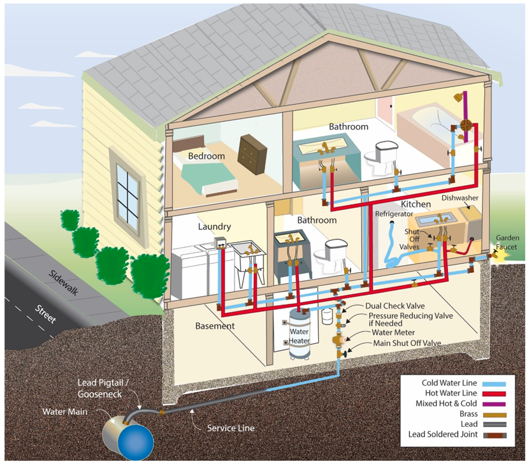
Illustrative premise plumbing configuration in a home. Water reaches outlets for consumptive and non-consumptive uses by following hot and cold lines specific to the plumbing design of each home. Redrawn and modified from https://www.finehomebuilding.com/membership/pdf/5798/021216063.pdf

2.2.1. Pb service lines and other Pb pipes

Major Pb sources in some US buildings (e.g., homes) are “legacy” Pb service lines (LSLs), Pb goosenecks, or other Pb-lined pipes (Fig. 3) which were installed prior to the 1986 US Pb ban and have not yet been replaced (Sandvig et al., 2008). These are made of pure Pb materials or pure Pb linings (100% Pb) and are often hidden underground or inside walls unbeknownst to residents. Service lines (or else communication pipes) are the specific pipes that connect premise plumbing to the water main, whereas goosenecks (or else pigtails) are shorter pipe segments connecting the service line to the water main (Figs. 2, 3). Houses without an LSL can still have unknown sections of Pb pipe inside the residence, or a Pb gooseneck connection to the main. In some areas of the US, particularly in the Northeast and Midwest, Pb-lined galvanized service lines and pipes were also used (Fig. 3).

Fig. 3.

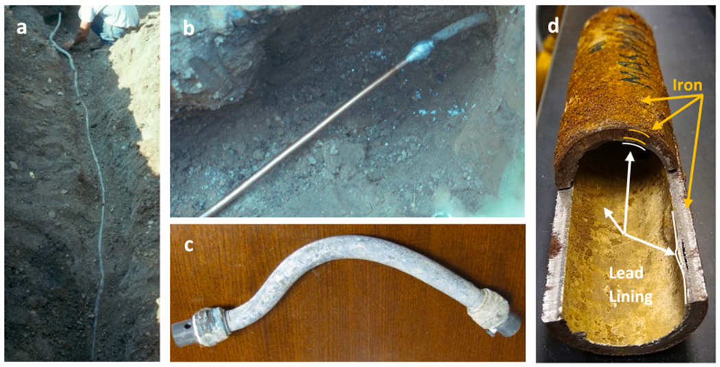
(a) Full lead service line in the ground, (b) privately-owned lead service line partially replaced by copper pipe with a wiped solder joint in the ground, (c) lead gooseneck that was excavated, (d) lead-lined iron service line that was excavated and cut open to expose the lead-lining.

In many systems, the highest water Pb levels originate from the LSL, but the degree of Pb release from LSLs may vary from house to house. For example, longer LSLs create a greater chance that the consumer may receive elevated water Pb at the tap. In a field study in Chicago, LSL length in sampled homes varied greatly between 43 and 159 feet (13–48 m), while the distance from the kitchen tap to the beginning of the LSL ranged from 3 to 87 feet (0.9–26.5 m) (Del Toral et al. 2013).

This variability depends on the premise (particularly kitchen) plumbing configuration and on the house location relative to the water main location (usually under the street). In some cases, LSLs are shorter because they enter a home at the front (Fig. 4, scenarios 1 and 2), whereas longer LSLs may enter at the back (Fig. 4, scenario 3). In addition, the location of the kitchen at the front (Fig. 4, scenario 1) or the back of a home (Fig. 4, scenarios 2 and 3) increases the distance from the primary Pb source (LSL) to the primary water consumption outlet (kitchen faucet). In other cases, homes with longer yards that are located further from the street or water main (Fig. 4, scenario i) or larger homes with larger premise plumbing systems (Fig. 4, scenario ii), may fall under any of the scenarios 4.1, 4.2, 4.3, further affecting LSL length and distance. The variable lengths and distances from kitchen taps to LSLs make it impossible to universally capture the Pb contribution from the LSL within a single water sample volume sequentially collected at the kitchen faucet (Del Toral et al., 2013; Deshommes et al., 2016; Hayes et al., 2013; Triantafyllidou et al., 2015).

Fig. 4.

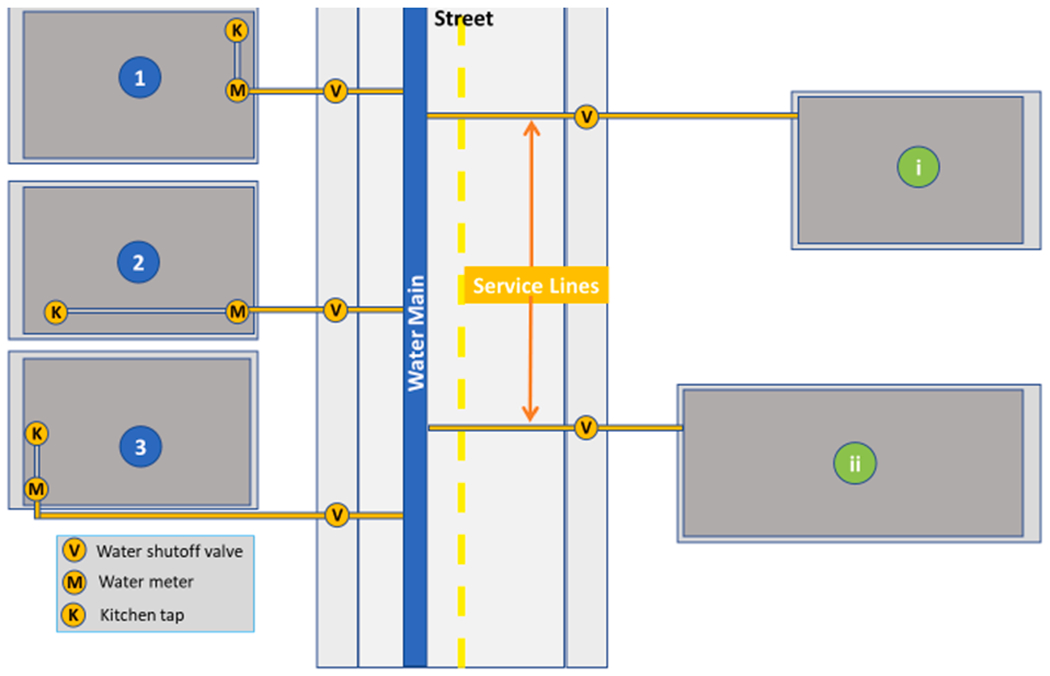
Illustrative schematic of the kitchen tap relative to the service line, for homes of different kitchen configurations (scenario 1–3). If home distance from the street varies and home size varies (scenarios i and ii), then the relative plumbing lengths are complicated further, depending on which kitchen configuration (scenario 1–3) applies. Modeled after Chicago (Del Toral et al., 2013), where the service line ends at the water meter which is typically located inside the home. In other cities the water meter can be outside of the home, and the configurations may be different.

2.2.2. Brass, bronze, Pb solder and galvanized pipes

Even with no pure Pb plumbing, buildings may still contain a wide array of fittings and devices containing Pb brass/bronze alloys (e.g., components in kitchen faucets or in water fountains, water meters, valves, elbows, ferrules) or Pb solder contributing Pb to water (AWWARF-TZW, 1996; AWWARF, 1990; Elfland et al., 2010; Karalekas et al., 1975; Sandvig et al., 2008; van den Hoven and Slaats, 2006). Such plumbing alloys have much lower Pb content relative to pure Pb sources but have been shown to release more Pb than LSLs in some water systems (Triantafyllidou et al. 2015).

Pb content was limited to less than 0.2% by weight in solder and to less than 8% by weight in brass in 1986 in the US (e-CFR 2020). The allowable Pb percentages were further modified to a 0.25% weighted average for wetted surfaces in order to meet the new “lead-free” requirement that took effect in 2014 (US Congress 2011). However, many houses and buildings retain “legacy” brass/bronze fittings and solders of higher Pb content from previous installations, whereas plumbing alloys with higher Pb content may still be illegally or unintentionally used in new buildings (Elfland et al., 2010; Triantafyllidou and Edwards, 2012).

Instances of high water Pb levels in buildings have been attributed to a legacy Pb brass ball valve (Elfland et al. 2010) or other Pb brass components (Government of Western Australia 2017) and to legacy Pb solder (Triantafyllidou and Edwards 2012). Even “lead-free” brasses containing a small percentage of Pb can potentially release consequential amounts of Pb into water. Current industry standards by NSF International did not anticipate the significant lowering of public health goals (e.g., the American Academy of Pediatrics 2016 recommendation of <1 μg/L Pb in school water). As a result, certified “lead-free” commercial plumbing products were found to leach Pb > 1 μg/L in one laboratory study (Parks et al. 2018).

Galvanized steel pipe can also be a source of Pb. The zinc lining contains 1% Pb that can leach into water (Leroy 1993), whereas the iron in the pipe can sorb Pb from upstream sources such as LSLs for eventual and substantial Pb release into drinking water even after the LSL has been removed (AWWARF-TZW, 1996; Clark et al., 2015; HDR, 2009; Hoekstra et al., 2004; McFadden et al., 2011; Pieper et al., 2017; Sandvig et al., 2008).

2.3. Lead temporal variability

The most understudied contributor to water Pb variability is arguably the impact of water use pattern, which determines the stagnation duration and pathways of flow as water contacts Pb-containing plumbing sources. Water use within buildings is intermittent and varies by the hour, day, and season due to resident schedule/lifestyle activities and weather. House age, number of residents and socioeconomic status all affect the frequency, duration, and intensity of water use (Buchberger and Wells, 1996; Del Toral et al., 2013). A list of questions on daily habits (Box 2) demonstrates how complex individual water use patterns can be.

Box 2.

Questions relating to building water use, as they may affect water movement in plumbing and subsequent Pb concentrations in water.

• How many people use water each day?

• What are the water uses, and in what order?

• Which water outlet is used, and when?

• How long did the water stand in which part(s) of the piping?

• What is the water pathway through the plumbing, each time a faucet or appliance is turned on?

• How much does the pattern of use vary from day to day, week to week, month to month?

• Are school or work-related activities the same or different from the prior day/week/month?

• Are there visitors who change the water use pattern?

The Water Research Foundation (WRF) reported that toilet flushing accounted for the largest indoor use of water in surveyed US single-family homes (24%), followed by faucets (20%), showers (20%), clothes washers (16%), leaks (13%), bathtubs (3%), other/miscellaneous (3%), and dishwashers (2%) (WRF 2016). Even if most of the demand is not-consumptive (i.e., not for drinking or cooking), any use causes water to move through the relevant plumbing branch and affects Pb levels in shared plumbing.

Hydraulic modeling of flow paths associated with different simulated water uses in an actual 3-level premise plumbing layout containing a 60-ft service line (Burkhardt et al. 2019), can provide insights into how water moves through a residence (Fig. 5). Collecting a 1-L cold water sample at the kitchen tap after stagnation does not capture water that stagnated within the LSL (Fig. 5b). Taking a warm shower (Fig. 5c) utilizes both hot and cold water, with the hot water quality impacted by the size of the hot water heater (Hawes et al. 2017). Like the 1 L sample, a 16-ounce (500 mL) glass of cold water (Fig. 5d) moves water along the same path, but only represents the first 13 feet (3.96 m) of plumbing. Even non-consumptive uses like watering the lawn (Fig. 5e) share plumbing branches with the kitchen faucet and may thus affect the Pb content in the next glass of water.

Fig. 5.

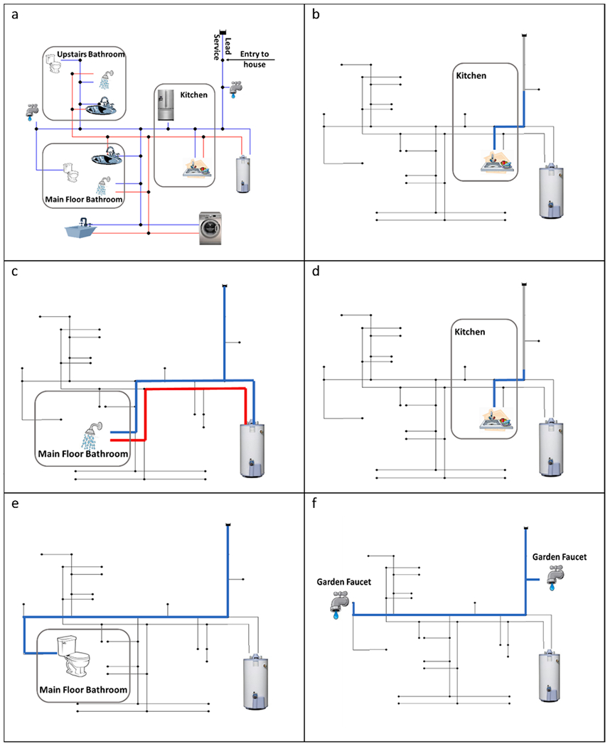
(a) Premise plumbing system simulated in EPANET, and water flow paths resulting from various assumed water uses: (b) collecting 1-L sample at kitchen tap after stagnation, (c) taking a warm shower, (d) collecting a 16-ounce (500 mL) glass of water, (e) flushing the toilet, (f) watering the lawn. Red/blue segments highlight water (hot/cold) that would be consumed by a given activity, whereas gray segments highlight water that would be moved. Remaining segments, not highlighted for a given activity, represent stagnant water which would not be directly impacted by the water activity. Not to scale. (For interpretation of the references to colour in this figure legend, the reader is referred to the web version of this article.)

Further illustrating these concepts, hydraulic modeling for a simpler linear LSL plumbing scenario demonstrated the mostly unrecognized impact of individual water use patterns to individual water Pb exposure (Table 2). Specifically, Murray (2017) demonstrated that drinking a glass of water did not move the Pb slug far enough from the LSL to affect the next glass of water. Brushing teeth or a 1.3-gallon (4.9 L) toilet flush moved the Pb slug enough to contaminate the next glass of water, whereas a shower or 3.6 gallon (13.6 L) toilet flush flushed out the Pb slug contained within the LSL, resulting in only a small residual Pb concentration at the tap.

Table 2.

Predicted Pb concentration in tap water depending on prior water use based on EPANET hydraulic modeling

Simulated water use	% LSL water slug moved by activity	Predicted Pb concentration in next glass of water at kitchen tap
8 oz (237 mL) glass of water	0% (Pb slug moved 2.7 ft or 0.8 m)	0 μg/L
Shower (17.2 Gal or 65 L @ 2 gpm)	100% (Pb slug flushed out)	4 μg/L
Toilet flush (3.6 Gal or 13.6 L @ 2 gpm)	100% (Pb slug flushed out)	4 μg/L
Toilet flush (1.3 Gal or 4.9 L @ 2 gpm)	50%	100 μg/L
Brushing teeth (1 Gal or 3.7 L)	20% (Pb slug moved 43.5 ft or 13.3 m)	100 μg/L

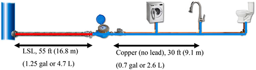Modeling assumptions: LSL (lead service line) is the only Pb source; Pb solubility in LSL set to 100 μg/L; Particulate Pb not incorporated; 8-h water stagnation in LSL before water use; ¾″ pipe diameters; water contained 0 μg/L Pb prior to use. Different assumptions/inputs would yield different predicted Pb concentrations, so the reader is encouraged to focus on the general trends instead.

Adapted from Murray (2017).

Riblet et al. (2019) recently filled some of the water use information gaps at 13 inhabited Canadian homes, by demonstrating that 50% of water uses drew less than 1 L from kitchen taps, with 92% of uses drawing less than 3 L. Elfland et al. (2010) and Nguyen et al. (2012) demonstrated the impact of water conservation devices (which in turn impact water use) at a university campus on water quality deterioration including water Pb contamination. DeSantis (2017) demonstrated the impact of extremes in occupancy to the total water use and measured water Pb levels in a US single-family midwestern home served by an LSL between 2007 and 2017. Total water usage in the home gradually decreased, as the number of residents decreased from 2 to 1 and ultimately to 0 over a decade. This caused Pb corrosion scale changes due to prolonged water stagnation within the LSL, which resulted in increased water Pb levels. That work brought attention to water quality in vacant/foreclosed buildings with LSLs and encouraged water sampling/remediation prior to reoccupation. By extension, the implications of prolonged under-occupancy or vacancy in some Pb-containing building plumbing networks due to grave circumstances (e.g., the COVID-19 pandemic shutdowns) should be considered, particularly in buildings like schools or daycares which eventually resume serving sensitive population groups (Proctor et al, 2020; US EPA, 2020).

3. Key water sampling components

Sample volume and water stagnation will be discussed here, but other key water sampling components have been reported elsewhere (Britton and Richards, 1981; Clark et al., 2014; Deshommes et al., 2010; Hoekstra et al., 2009; Masters et al., 2016b; Triantafyllidou and Edwards, 2012; van den Hoven and Slaats, 2006).

3.1. Water sample volume

The volume of water sampled in standard sampling containers (30 mL, 60 mL, 125 mL, 250 mL, 500 mL, 1 L, etc) essentially equals plumbing distance from the sampled water outlet (i.e., volume = distance), as determined by pipe material and internal pipe diameter (Schock and Lytle, 2011; Vaccari, 1994). For example, collecting one liter of water coming out of a tap after stagnation, corresponds to 17–26 feet (5.2–7.9 m) of plumbing distance depending on pipe material, for a typical home pipe internal diameter of ½ inch (Fig. 6). Such volume/distances will capture water contained within the faucet and an associated short section of premise plumbing, impacted by a variety of proximal plumbing devices and materials. But they will not capture distal Pb plumbing sources, such as an LSL or Pb gooseneck.

Fig. 6.

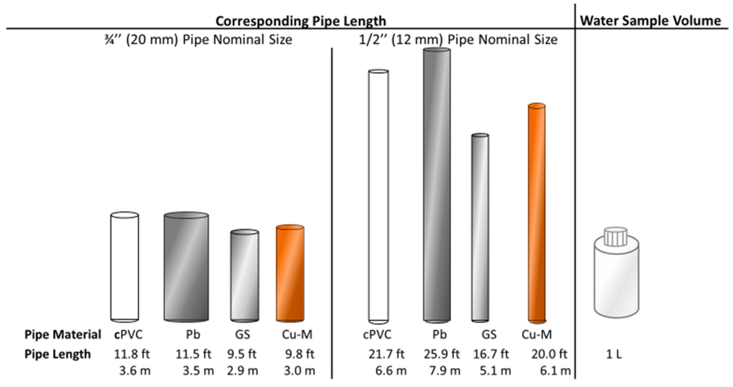
Correspondence of one liter of water sample volume to pipe length, for typical pipe materials and nominal sizes. cPVC: Chlorinated Polyvinylchloride, Pb: lead, GS: Galvanized steel, Cu-M: Copper type M. Not to scale. Note: GS pipe may undergo severe corrosion (i.e., tuberculation) that can substantially decrease internal diameter.

The sample volume can also cause dilution effects (Cardew, 2000; Del Toral et al., 2013; Hayes et al., 2013). For example, a one-liter water sample may dilute the small volume of Pb-contaminated water within a leaded kitchen brass faucet, which was found to range between 56 and 135 mL (Gardels and Sorg 1989), 65–150 mL (Maas et al. 1992) and 24–233 mL (Cartier et al. 2012). Considering that water volumes may vary significantly between kitchen faucets, bubblers in water fountains, laboratory faucets used in US schools/hospitals, and janitor/utility sink faucets; a one-size-fits-all approach (like 1 L or 250 mL sample volume) cannot answer all the questions surrounding Pb in drinking water (see subsequent section on Sampling Protocols).

3.2. Stagnation

The duration of water stagnation prior to sampling is important, because Pb diffuses quickly from Pb pipe within the first few hours of stagnation and will eventually reach a concentration equilibrium peak (Doré et al., 2019; Schock, 1990). However, long stagnation periods are difficult to achieve because they require no water use throughout the entire house/building for an extended period of time (Hoekstra et al., 2009; Schock and Lemieux, 2010). Even non-consumptive water uses, including flushing toilets, furnace humidifiers, lawn sprinklers or accidental leaks can compromise water stagnation and the subsequently collected water sample.

Inter-use stagnation, i.e. the time between each water use at the kitchen tap by residents, was estimated at 30 min on average by earlier European studies (van den Hoven and Slaats 2006). This is typically much shorter than the long stagnation required for Pb to reach its peak concentration. The range of inter-use stagnation at kitchen taps in one Canadian study was recently reported between <15 min (47% frequency) to >6 h (10% frequency) (Riblet et al. 2019).

4. Sampling protocols

Sampling protocols for Pb in water can be classified under three general categories depending on their ability to answer specific questions related to Pb in water (Table 3). Brief descriptions for our classification are provided below, whereas other detailed explanations and classifications are also available to the reader (Hoekstra et al., 2009; van den Hoven and Slaats, 2006).

Table 3.

Sampling protocols for lead in drinking water that have been used to meet different objectives. The list is not meant to be exhaustive.

Sample type	Sample protocol summary	objective & question(s) answered
First Draw (FD), US – 90th percentile Pb < 15 μg/L	– Overnight water stagnation (6+ hr) – Collect 1 L	1. Lead regulatory compliance in a certain jurisdiction: • Does the water meet a regulatory standard for Pb?
Random Daytime (RDT), UK – 95th percentile Pb < 10 μg/L	– Collect during random work hours (i.e., variable stagnation) – Collect 1 L
30 Min. Stagnation (30MS), Ontario Canada – Pb < 10 μg/L (5 μg/L considered)	– 2 to 5 min. preflush – 30 min. stagnation – Collect first two liters & average Pb results
Profile (or else sequential)	– Defined stagnation time – Collect 10 to 20 sequential samples of defined volume (125 mL, 250 mL, 1 L, etc.)	2. Lead plumbing sources determination and/or lead form identification:
Fully flushed	– No stagnation – Flush out several piping volumes – Collect 1 L	• Where is the Pb coming from?
School guidance, US	– Overnight stagnation (8–18 hr) – Collect first 250 mL from all taps and fountains
Particle stimulation	– Profile sampling repeated at increasingly higher water flow rate: low, medium, and high flow rate, or alternatively – 5 min stagnation – Collect first liter at maximum flow rate, open and close tap five times, fill rest of bottle at normal flow rate – Collect second liter at a normal flow rate – Collect third liter the same way as the first	– What form of Pb is present (dissolved/ particulate)?
RDT	– Collect statistically sufficient RDT samples (explained above) at homes across community	3. Average Pb Exposure Assessment at community level or household level • What is the average exposure to Pb in water in this community?
Composite proportional (automatic or manual)	– Sampling device diverts fixed proportion (e.g., 5%) of water every time water is drawn for consumption – Cumulative water samples may even be collected manually at each water consumption event (typically no more than 3 L) – Over extended period of time (e.g., 1 day to 1–2 weeks)	• What is the average exposure to Pb in water in this household?

4.1. Single sample protocols

Several protocols consist of taking a single water sample from a building faucet or fountain. First-Draw (FD) is a single fixed-volume sample taken after long stagnation (e.g., overnight) that produces time-amplified “worst case” Pb concentration for the segment of piping sampled, when Pb release approaches its equilibrium peak (Lytle and Schock 2000). Random Daytime (RDT) is another single fixed-volume sample, but taken without any stagnation at a random time during the workday, which is impacted by the random residential water use pattern (Hayes and Hydes 2012). 30-Minute Stagnation (30 MS) is a single fixed-volume sample taken after pre-flushing and subsequent 30-minute stagnation which captures the average 30-minute inter-use stagnation time identified in older European studies (Cardew, 2003; van den Hoven and Slaats, 2006).

These single sample protocols are simple/practical to employ across many homes for system-wide compliance with a water Pb regulatory standard (Table 3), but they are not meant to provide direct water Pb exposure information for individual households, nor can they precisely identify all Pb plumbing sources and their relative importance. For instance, the US compares the 90% percentile of FD samples against a 0.015 mg/L (15 μg/L) action level (which is not meant to be a health-based standard) under the 1991 Lead and Copper Rule (e-CFR 2020) that is currently under revision (US Federal Register 2019). The UK compares the 95% percentile of RDT samples against the 10 μg/L World Health Organization’s provisional tolerable weekly intake of Pb for children (WHO 2008) under its Drinking Water Directive (Drinking Water Inspectorate 2010). The Province of Ontario, Canada compares 30 MS samples to Health Canada’s prior Pb maximum acceptable concentration (MAC) of 10 μg/L (Government of Ontario 2002). An overview of regulatory approaches in other Canadian provinces can be found elsewhere (Dore et al. 2018).

4.2. Sequential (or Profile) sampling

Unlike the previous single samples, profile sampling collects many sequential water samples from the same kitchen faucet, after a prescribed stagnation period (Clark et al., 2014; Del Toral et al., 2013; Lytle et al., 2019; Vaccari, 1994). The required number and incremental volumes of sequential samples to ultimately capture the full volume of water between the kitchen faucet and the water main depends on the specific plumbing network. Thus, conducting an individual premise plumbing assessment can be very useful, albeit time-consuming. A sampling plan developed for a particular building may not provide meaningful information if used for another building with different plumbing materials, configurations and dimensions (i.e., lengths and internal diameters of segments) (see previous section on Factors affecting Pb variability in drinking water).

In general, smaller sample volumes can be taken initially (e.g., 30 mL, 60 mL, 125 mL) to provide more spatial resolution and pinpoint specific proximal small sources of Pb like brass faucet/water fountain components, a brass valve, or a Pb soldered copper joint (Hoekstra et al., 2004; Lytle et al., 2019; Vaccari, 1994), since larger samples may reflect multiple small Pb components (Fig. 7). Larger sample volumes (e.g., 1 L) taken subsequently can capture distal larger Pb segments like LSLs or Pb goosenecks.

Fig. 7.

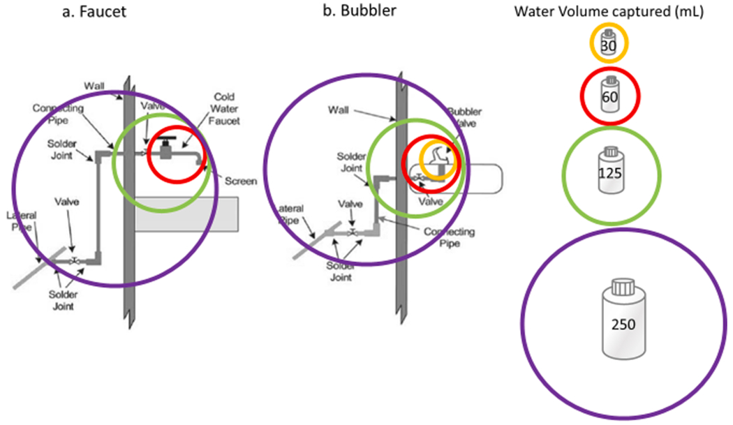
Estimated correspondence between water sample volume and Pb plumbing source in example configurations of a) water faucet, and b) water bubbler. Sample volumes were overlaid on top of schematics from the US EPA’s 3Ts guidance (2018). Specific brands/models may differ from the estimated correspondences illustrated here.

Sequential sampling results create a profile of Pb concentration versus water sample volume (where water volume = plumbing distance), which can help identify Pb sources along the plumbing line, especially LSL peaks (Clark et al., 2014; Del Toral et al., 2013; Deshommes et al., 2017; Lytle et al., 2019; Sandvig et al., 2008; van den Hoven and Slaats, 2006). While expensive/cumbersome due to the numerous samples, sequential sampling is the most comprehensive approach for Pb plumbing source determination (Table 3). Sequential sampling further evolved to incorporate high sampling flow rates for particle stimulation (Table 3), that better capture particulate Pb in water due to scouring (Clark et al. 2014). Profile sampling helps to answer the question of where the Pb is coming from, and in what form if high sampling flow rate is incorporated, so that it can be removed/remediated. However, it does not directly answer the question of Pb ingestion exposure in the sampled building.

4.3. Pb exposure sampling

Determining human exposure to Pb at the tap is the most complex water sampling endeavor, because the sampling protocol must capture Pb spatial and temporal variability under typical water use over a period of time. Further, assessing average water Pb potential exposure at the community level is different than average Pb potential exposure at the individual resident or household level.

4.3.1. Community assessment of water Pb exposure

Single-sample protocols (Table 3) do not represent average water Pb consumption in individual households (Hayes, 2009; Hoekstra et al., 2008). For instance, FD captures one worst-case stagnation scenario out of the infinitely numerous water stagnation possibilities (Cartier et al. 2011), whereas 30 MS captures one estimate of the average inter-use stagnation time (Jackson 2000). Single RDT in a home captures one random water use pattern during the workday.

If a statistically sufficient number of single RDT samples is collected throughout homes of a community, then a range of inter-use stagnation times can be captured to approximate average water Pb exposure in that community (Cardew, 2003; Cartier et al., 2011; Sandvig et al., 2008; Schock, 1990). The RDT approach may therefore be suitable for assessment of average water Pb exposure system-wide but not in individual homes. Conceptually however, many RDT samples collected in the same home over time may statistically approximate average water Pb exposure in that home, although this concept requires further exploration to avoid potential biases.

Comparative studies in different countries reached different conclusions regarding the best single-sample protocol for approximating system-wide average water Pb exposure (Riblet et al., 2019; van den Hoven et al., 1999), but they used a reference protocol for their comparison, namely composite proportional sampling.

4.3.2. Household assessment of water Pb exposure

Composite proportional sampling was developed in the late 1970s in the Netherlands (Haring, 1984; van den Hoven, 1987) by attaching a sampling device to the kitchen tap that diverts a fixed percentage of water, usually 3–5%, into a large sampling bottle each time water is drawn for consumption and the user flips the side-stream diversion switch (Fig. 8) (Anjou Recherche, 1994; van den Hoven and Slaats, 2006). After a defined period, usually ranging from one day (Clement et al. 2000) to one or two weeks (Riblet et al. 2019), the resulting composite water sample is analyzed to produce an average water Pb concentration. The total water volume consumed can also be estimated, so that the average Pb exposure dose (i.e., average Pb mass that would be ingested over that period) can be calculated. The composite sample is considered more representative of average Pb exposure than any of the single samples, because it directly samples an approximate average water Pb concentration over a prolonged period of normal household water use.

Fig. 8.

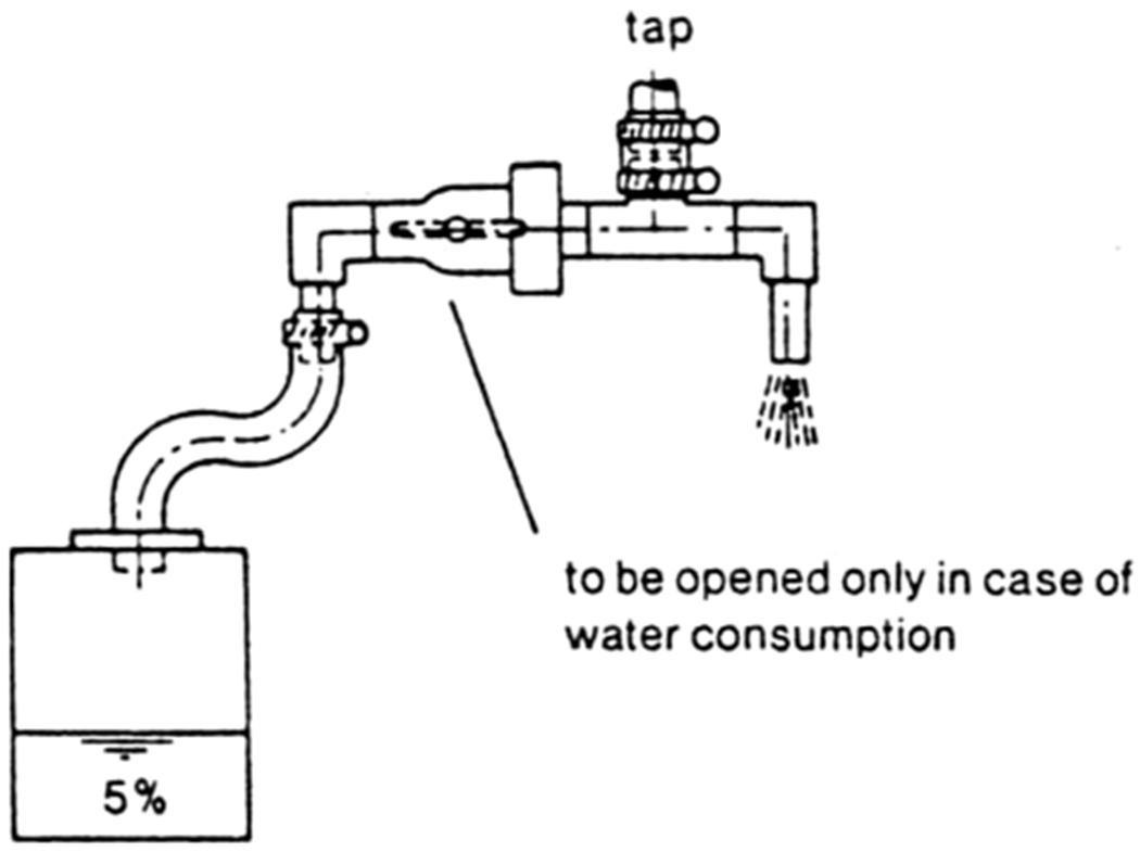
Composite proportional sampling device. Reprinted from Aqua 1987 vol 6, van den Hoven. A New Method to Determine and Control Lead Levels in Tap Water. Copyright (2004).

The composite proportional devices must be designed and oriented in a way that accurately captures particulate lead. The user-operated proportional sampling devices are considered inconvenient and cumbersome by residents (Clement et al., 2000; Meranger and Subramanian, 1984) with the possibility of improper use (Hoekstra et al. 2009). Additionally, due to the needed sampling device, extra counter space and longer duration, this sampling protocol can be more expensive than other sampling protocols and was not deemed suitable for community sampling (van den Hoven 1987).

Manual composite sampling is a simpler approach dating back to the 1970s, when researchers collected a quart (i.e., 0.95 L) of water from the kitchen tap every night at dinner (Karalekas et al. 1975), or at each meal (Greathouse et al., 1976; Worth et al., 1981) or other variations of water volume/timing of sampling that focused on water consumption of bottle-fed infants (Lacey et al., 1985; Sherlock and Quinn, 1986). Schock et al. (2019) recently proposed returning to this approach, by collecting a pre-determined amount of water each time the water is drawn for drinking or cooking and accumulating that water for a specific amount of time in a large container for subsequent Pb analysis of the cumulative water volume. This simpler manual approach does approximately capture the cumulative water Pb concentration by simple analysis of the composite sample. But it does not precisely track the total water volume because it collects identical water volumes at each water use, unlike the composite proportional sampling device which captures percentages and can thus back-calculate more precisely the total water volume consumed. Jarvis et al. (2018) collected sub-samples from each measured drink consumed at home over three days. They used a measuring cup to record water volume before it was consumed and analyzed the sub-samples rather than a composite water sample, which is more precise but more costly/cumbersome.

Composite Pb accumulation passive sampling is a theoretical approach mentioned by Cantor et al. (2013). A variation of it was somewhat explored by Deshommes et al. (2017), although it was explored at the household point of entry and not the point of use in that study. It is currently under development/refinement (Lytle and Schock 2019) and thus not included in Table 3 because it is not currently used in practice. It is based on the ability of appropriately certified point of use (POU) filtration devices to remove soluble and particulate Pb from water at the tap used for consumption (cooking and drinking). Rather than actively sampling water, Pb in the drinking water that passes through the faucet-mounted POU device is trapped on the filtration media and concentrates over time. At the end of the filter’s service life (or some specified volume of filtered water), the filter cartridge can be removed from the device and the Pb can be extracted from the filter media.

If the POU device has a flow totalizer that tracks the total volume of water that passes the device, then an average Pb concentration can be calculated by dividing the Pb mass extracted (μg Pb) by the volume filtered (liters). Since only water for consumption passes the sampling device, the final concentration reasonably reflects exposure. Ultimately, the premise of this approach relies on the ability to quantitatively extract the accumulated Pb from the POU filtration media. It warrants further exploration, with Pan et al. (2020) recently reporting promising results from various POU filter Pb extraction approaches.

Although not perfect, composite Pb accumulation passive sampling is conceptually more representative of average Pb exposure than other protocols, as is composite proportional sampling. However, the average Pb exposure calculated from one week of sampling may still not be representative of Pb exposure throughout the year (Hoekstra et al. 2004), because of the aforementioned variations in water corrosivity coupled with different work or recreational patterns from day to day, week to week, or over the year. Therefore, potential exposure will vary over time, and multiple composite sampling events would ideally be needed to obtain the most realistic and accurate estimates.

Even within a household, individual residents will not have the same water Pb exposure, because of the many variables previously discussed. Sampling to isolate individual Pb potential exposure is almost impossible, unless individual water consumption patterns can be separated from the rest of the household such as in the case of formula-fed infants in Lacey et al. (1985). It is important to mention that exposure to water Pb is a combination of drinking water consumption inside and outside the home (e.g., at daycare, school, or at work), which further complicates matters. Still, the resolution of the composite proportional sampling or composite Pb accumulation passive sampling goes down to capturing average water Pb potential exposure at the household level, which is an advancement over single-sample protocols that are intended for other purposes.

5. Discussion

Review of the literature yielded the following conclusions:

• Residential water sampling for Pb assessment is a flexible tool with many purposes. No single universally applicable sampling protocol exists, and each protocol has a specific use toward answering one or more questions relevant to Pb in water.

• Understanding the inherent variabilities (spatial and temporal) of Pb release into drinking water is essential to accurate data interpretation for a given sampling intention, particularly for the complex task of exposure estimation. For instance, water Pb regulatory sampling protocols employ practical single samples that were not meant to estimate potential water Pb exposure at the household level, nor were they all necessarily intended to relate to health-based Pb standards. Few sampling protocols are designed to approximate human exposure by Pb ingestion through water.

• Different water sampling protocols (including different sample volumes under otherwise identical sampling instructions) will yield different Pb concentrations from different sources/forms of Pb. Understanding the detailed differences in sampling protocols is critically important when comparing existing Pb results from different studies.

• In order to establish statistical correlations of drinking water Pb concentrations to blood Pb measurements or to predict/estimate blood Pb levels from existing datasets, the limitations of available drinking water Pb datasets in representing water Pb exposure need to be understood and the uncertainties need to be discussed (as was done in Stanek et al., 2020; Zartarian et al., 2017). Sampling biases may relate poorly to the probable amount of Pb ingestion and may underestimate or overestimate the impact of water Pb ingestion on blood Pb.

Review of the literature yielded the following recommendations:

• Caution is advised when loosely using the term “exposure assessment” for all water Pb sampling protocols, given that most sampling protocols cannot accurately represent Pb exposure. This is especially important in relatively rare events causing acute Pb exposures, as explained in Triantafyllidou and Edwards (2012).

• Health professionals are encouraged to explore water sampling protocols that better capture household water Pb potential exposures during environmental assessments of Pb-poisoned children. That could potentially uncover a previously unknown water Pb problem as contributing to elevated blood Pb. Currently, health departments in the US may not test the water for Pb at all during a home evaluation. If water is tested, health departments follow common single-sample protocols that were developed for other purposes such as regulatory sampling, in the absence of other guidance (Triantafyllidou and Edwards 2012).

• The complexities brought up are not meant to discourage measurement of Pb in drinking water. It is understandable that practical considerations including sampling costs, simplicity, timeliness and consumer acceptance need to be factored in when selecting an appropriate sampling protocol. Future study designs for estimating the relationship of drinking water Pb to Pb exposure need to carefully balance the logistics of data collection with the benefits/limitations of different sampling protocols. It will likely be necessary to establish clear limitations/caveats to the ability to extrapolate from much of the existing Pb water data, as well.

References

- AWWARF-TZW, 1996. Internal corrosion of water distribution systems. Second ed Denver, CO: AWWA Research Foundation/DVGW-TZW. [Google Scholar]
- Anjou Recherche, 1994. Etude des phenomenes de solubilisation du plomb par l’eau distribuee et des moyens pour les limiter. Compagnie Generate Des Eaux, Paris. [Google Scholar]
- AWWARF, 1990. Lead control strategies. AWWA Research Foundation and AWWA, Denver, CO. [Google Scholar]
- Beattie AD, Moore MR, Devenay WT, Miller AR, Goldberg A, 1972. Environmental lead pollution in an urban soft-water area. BMJ 2, 492–493 bmj.com/content/2/5812/491. [DOI] [PMC free article] [PubMed] [Google Scholar]
- Britton A, Richards WN, 1981. Factors influencing plumbosolvency in Scotland. J. Inst. Water Engrs. Sci 35, 349–364. [Google Scholar]
- Buchberger SG, Wells GJ, 1996. Intensity, duration, and frequency of residential water demands. J. Water Resour. Plann. Manage 122 10.1061/(ASCE)0733-9496(1996)122:1(11). [DOI] [Google Scholar]
- Burkhardt J, Woo H, Mason J, Platten W, Murray R, 2019. Modeling water age in premise plumbing systems. In: Proceedings of the World Environmental & Water Resources Congress, EWRI, ASCE; Pittsburgh, PA. [Google Scholar]
- Cantor AF, Maynard BJ, Hart P, Kapellusch AM, et al. 2013. Application of filters for evaluating lead and copper concentrations in tap water, Water Research Foundation web report #4415. https://www.waterrf.org/research/projects/application-filters-evaluating-lead-and-copper-concentrations-tap-water (accessed January 15 2020).
- Cardew PT, 2000. Simulation of lead compliance data. Water Res. 34, 2241–2252. 10.1016/S0043-1354(99)00411-X. [DOI] [Google Scholar]
- Cardew PT, 2003. A method for assessing the effect of water quality changes on plumbosolvency using random daytime sampling. Water Res. 37, 2821–2832. 10.1016/S0043-1354(03)00120-9. [DOI] [PubMed] [Google Scholar]
- Cartier C, Laroche L, Deshommes E, Nour S, Richard G, Edwards M, Prevost M, 2011. Investigating dissolved lead at the tap using various sampling protocols. J. AWWA 103, 55–67. 10.1002/j.1551-8833.2011.tb11420.x. [DOI] [Google Scholar]
- Cartier C, Nour S, Richer B, Deshommes E, Prévost M, 2012. Impact of water treatment on the contribution of faucets to dissolved and particulate lead release at the tap. Water Res. 46, 5205–5216. 10.1016/j.watres.2012.07.002. [DOI] [PubMed] [Google Scholar]
- Clark B, Masters S, Edwards M, 2014. Profile sampling to characterize particulate lead risks in potable water. Environ. Sci. Technol 48, 6836–6843. 10.1021/es501342j.. [DOI] [PubMed] [Google Scholar]
- Clark BN, Masters SV, Edwards MA, 2015. Lead release to drinking water from galvanized steel pipe coatings. Environ. Eng. Sci 32, 713–721. 10.1089/ees.2015.0073. [DOI] [Google Scholar]
- Clement M, Seux R, Rabarot S, 2000. A practical model for estimating total lead intake from drinking water. Water Res. 34, 1533–1542. 10.1016/S0043-1354(99)00277-8. [DOI] [Google Scholar]
- Davies DJ, Thornton I, Watt JM, Culbard EB, Harvey PG, Delves HT,Sherlock JC, Smart GA, Thomas JF, Quinn MJ, 1990. Lead intake and blood lead in two-year-old U.K. urban children. Sci. Total Environ 90, 13–29. 10.1016/0048-9697(90)90182-t. [DOI] [PubMed] [Google Scholar]
- Del Toral MA, Porter A, Schock MR, 2013. Detection and evaluation of elevated lead release from service lines: A field study. ES&T 47:9300–9307. 10.1021/es4003636. [DOI] [PubMed] [Google Scholar]
- DeSantis MK, 2017. Conversion of lead corrosion scale under changing redox conditions. In: Proceedings of the AWWA Annual Conference and Exposition, June 11-14 2017 Philadelphia, PA. [Google Scholar]
- Deshommes E, Laroche L, Nour S, Cartier C, Prévost M, 2010. Source and occurrence of particulate lead in tap water. Water Res. 44, 3734–3744. 10.1016/j.watres.2010.04.019.. [DOI] [PubMed] [Google Scholar]
- Deshommes E, Prevost M, Levallois P, Lemieux F, Nour S, 2013. Application of lead monitoring results to predict 0–7 year old children’s exposure at the tap. Water Res. 47, 2409–2420. 10.1016/j.watres.2013.02.010.. [DOI] [PubMed] [Google Scholar]
- Deshommes E, Bannier A, Laroche L, Nour S, Prévost M, 2016. Monitoring-based framework to detect and manage lead water service lines. J. Am. Water Works Assoc 108 (11), E555–E570. 10.5942/jawwa.2016.108.0167. [DOI] [Google Scholar]
- Deshommes E, Laroche L, Deveau D, Nour S, Prévost M, 2017. Short- and long-term lead release after partial lead service line replacements in a metropolitan water distribution system. ES&T 51(17), 9507–9515. , 10.1021/acs.est.7b01720. [DOI] [PubMed] [Google Scholar]
- Deshommes E, Trueman B, Douglas I, Huggins D, Laroche L, Swertfeger J, Spielmacher A, Gagnon GA, Prévost M, 2018. Lead levels at the tap and consumer exposure from legacy and recent lead service line replacements in six utilities. Environ. Sci. Technol 52, 9451–9459. 10.1021/acs.est.8b02388. [DOI] [PubMed] [Google Scholar]
- Dore E, Deshommes E, Andrews RC, Nour S, Prevost M, 2018. Sampling in schools and large institutional buildings: Implications for regulations, exposure and management of lead and copper. Water Res. 140, 110–122. 10.1016/j.watres.2018.04.045.. [DOI] [PubMed] [Google Scholar]
- Doré E, Deshommes E, Laroche L, Nour S, Prévost M, 2019. Lead and copper release from full and partially replaced harvested lead service lines: Impact of stagnation time prior to sampling and water quality. Water Res. 150, 380–391. 10.1016/j.watres.2018.11.076. [DOI] [PubMed] [Google Scholar]
- e-CFR, 2020. Title 40: Protection of environment, part 141—national primary drinking water regulations, subpart i—control of lead and copper. https://www.ecfr.gov/cgi-bin/text-idx?SID=e2518c71584f661373492ec68f3f6660&mc=true&node=sp40.25.141.i&rgn=div6 (accessed April 23 2020).
- Edwards M, Triantafyllidou S, Best D, 2009. Elevated blood lead in young children due to lead-contaminated drinking water: Washington, DC, 2001–2004. ES&T 43: 1618–1623. 10.1021/es802789w. [DOI] [PubMed] [Google Scholar]
- Edwards M, 2014. Fetal death and reduced birth rates associated with exposure to lead-contaminated drinking water. Environ. Sci. Technol 48, 739–746. 10.1021/es4034952. [DOI] [PubMed] [Google Scholar]
- Elfland C, Scardina P, Edwards M, 2010. Lead-contaminated water from brass plumbing devices in new buildings. J. AWWA 102, 66–76. 10.1002/j.1551-8833.2010.tb11340.x. [DOI] [Google Scholar]
- Elwood PC, St Léger AS, Morton M, 1976. Dependence of Blood-lead on domestic water lead. The Lancet 307, 1295 10.1016/S0140-6736(76)91763-3. [DOI] [PubMed] [Google Scholar]
- Fertmann R, Hentschel S, Dengler D, Janssen U, Lommel A, 2004. Lead exposure by drinking water: an epidemiological study in Hamburg, Germany. Int. J. Hyg. Environ. Health 207 (3), 235–244. 10.1078/1438-4639-00285.. [DOI] [PubMed] [Google Scholar]
- Etchevers A, Le Tertre A, Lucas JP, Bretin P, Oulhote Y, Le Bot B, Glorennec P, 2015. Environmental determinants of different blood lead levels in children: A quantile analysis from a nationwide survey. Environ. Int 74, 152–159. 10.1016/j.envint.2014.10.007.. [DOI] [PubMed] [Google Scholar]
- Gardels MC, Sorg TJ, 1989. A laboratory study of the leaching of lead from water faucets. J. AWWA 81,101–113. 10.1002/j.1551-8833.1989.tb03245.x. [DOI] [Google Scholar]
- Government of Ontario, 2002. Ontario regulation 170/3 drinking water systems, https://www.ontario.ca/laws/regulation/r03170 (accessed January 15 2020).
- Government of Western Australia, 2017. An audit of contractor and product performance in the construction of the new Perth children’s hospital, https://www.commerce.wa.gov.au/sites/default/files/atoms/files/final_report_-_perth_childrens_hospital_audit.pdf (accessed April 20 2020).
- Greathouse DG, Craun GF, Worth DJ, 1976. Epidemiological study of the relationship between lead in drinking water and blood lead levels. In: Proceedings of the Toxic Substances in Environmental Health-X, pp. 9–24. [Google Scholar]
- Hanna-Attisha M, LaChance J, Sadler RC, Champney Schnepp A, 2016. Elevated blood lead levels in children associated with the Flint drinking water crisis: A spatial analysis of risk and public health response. Am. J. Public Health e1–e8. 10.2105/AJPH.2015.303003. [DOI] [PMC free article] [PubMed] [Google Scholar]
- Haring BJA, 1984. Lead in drinking water. PhD Dissertation University of Amsterdam. [Google Scholar]
- Hawes JK, Conkling EA, Casteloes KB, Brazeau RH, Salehi M, Whelton AJ, 2017. Predicting contaminated water removal from residential water heaters under various flushing scenarios. J. – Am. Water Works Assoc 109, E332–E342. 10.5942/jawwa.2017.109.0085. [DOI] [Google Scholar]
- Hayes CR, 2009. Computational modelling to investigate the sampling of lead in drinking water. Water Res. 43, 2647–2656. 10.1016/j.watres.2009.03.023. [DOI] [PubMed] [Google Scholar]
- Hayes CR, Hydes OW, 2012. UK experience in the monitoring and control of lead in drinking water. J. Water Health 10 (3), 337–348. 10.2166/wh.2012.210.. [DOI] [PubMed] [Google Scholar]
- Hayes CR, Croft TN, Campbell JA, Douglas IP, Gadoury PJ, Schock MR, 2013. Optimization of corrosion control for lead in drinking water using computational modeling techniques. J. NEWWA. [Google Scholar]
- HDR Inc., 2009. An analysis of the correlation between lead released from galvanized iron piping and the contents of lead in drinking water. Bellevue, WA. [Google Scholar]
- Hoekstra EJ, Pedroni V, Passarella R, Trincherini PR, Eisenreich SJ, 2004. Elements in tap water part 3: Effect of sample volume and stagnation time on the concentration of the element. EUR 20672 EN/3. [Google Scholar]
- Hoekstra EJ, Aertgeerts R, Bonadonna L, Cortvriend J, Drury D, Goossens R, et al. , 2008. The advice of the ad-hoc working group on sampling and monitoring to the standing committee on drinking water concerning sampling and monitoring for the revision of the council directive 98/83/ec. EUR 23374 EN. [Google Scholar]
- Hoekstra EJ, Hayes CR, Aertgeerts R, Becker A, Jung M, Postawa A, et al. , 2009. Guidance on sampling and monitoring for lead in drinking water. EUR 23812 EN - 2009.European Commission Joint Research Centre, Institute for Health and Consumer Protection. [Google Scholar]
- Drinking Water Inspectorate. 2010. Guidance on the implementation of the water supply (water quality) regulations 2000 (as amended) in England. [Google Scholar]
- Jackson P, 2000. Monitoring the performance of corrective treatment methods. WRc-NSF Ltd, Oakdale, Gwent, UK. [Google Scholar]
- Jarvis P, Quy K, Macadam J, Edwards M, Smith M, 2018. Intake of lead (Pb) from tap water of homes with leaded and low lead plumbing systems. Sci. Total Environ 644, 1346–1356. 10.1016/j.scitotenv.2018.07.064. [DOI] [PubMed] [Google Scholar]
- Karalekas PC, Craun GF, Hammonds AF, Ryan CR, Worth DJ, 1975. Lead and other trace metals in drinking water in the Boston metropolitan area In: Proceedings of the AWWA 95th Annual Conference Minneapolis, Minnesota. [Google Scholar]
- Kim EJ, Herrera JE, Huggins D, Braam J, Koshowski S, 2011. Effect of pH on the concentrations of lead and trace contaminants in drinking water: A combined batch, pipe loop and sentinel home study. Water Res. 45, 2763–2774. 10.1016/j.watres.2011.02.023. [DOI] [PubMed] [Google Scholar]
- Kuch A, Wagner I, 1983. Mass transfer model to describe lead concentrations in drinking water. Water Res. 17, 1303 10.1016/0043-1354(83)90256-7. [DOI] [Google Scholar]
- Lacey RF, Moore MR, Richards WN, 1985. Lead in water, infant diet and blood: The Glasgow duplicate diet study. Sci. Total Environ 41, 235–257. 10.1016/0048-9697(85)90144-5. [DOI] [PubMed] [Google Scholar]
- Lanphear BP, Weitzman M, Winter NL, Eberly S, Yakir B, Tanner M, Emond M, Matte TD, 1996a. Lead-contaminated house dust and urban children’s blood lead levels. Am. J. Public Health 86, 1416–1421, 10.2105%2Fajph.86.10.1416. [DOI] [PMC free article] [PubMed] [Google Scholar]
- Lanphear BP, Weitzman M, Eberly S, 1996b. Racial differences in environmental exposures to lead. Am. J. Public Health 86, 1460–1463. . [DOI] [PMC free article] [PubMed] [Google Scholar]
- Laxen DP, Raab GM, Fulton M, 1987. Children’s blood lead and exposure to lead in household dust and water-a basis for an environmental standard for lead in dust. Sci. Total Environ 66, 235–244. 10.1016/0048-9697(87)90091-X. [DOI] [PubMed] [Google Scholar]
- Leroy P, 1993. Lead in drinking water: Origins; solubility; treatment. Aqua AQUAAA 42. [Google Scholar]
- Levallois P, St-Laurent J, Gauvin D, Courteau M, Prévost M, Campagna C, Lemieux F, Nour S, D’Amour M, Rasmussen PE, 2014. The impact of drinking water, indoor dust and paint on blood lead levels of children aged 1–5 years in Montreal (Quebec, Canada). J. Expo. Sci. Environ. Epidemiol 24 (2), 185–191. 10.1038/jes.2012.129.. [DOI] [PMC free article] [PubMed] [Google Scholar]
- Lytle D, Schock M, Wait K, Cahalan K, Bosscher V, Porter A, et al. , 2019Sequential drinking water sampling as a tool for evaluating lead in Flint, Michigan. Water Res. 40–54. 10.1016/j.watres.2019.03.042. [DOI] [PMC free article] [PubMed] [Google Scholar]
- Lytle DA, Schock M, 2000. Impact of stagnation time on metal dissolution from plumbing materials in drinking water. J. Water Supply: Res. Technol 49, 243–257. 10.2166/aqua.2000.0021. [DOI] [Google Scholar]
- Lytle DA, Schock MR, 2019. Lead exposure assessment device (LEAD). U.S. Patent application publication number: 20190100443.
- Maas RP, Patch SC, Peek BT, Brown GM, 1992. Standardized lead leaching characteristics of twenty-one models of new faucet fixtures and instant hot water dispensers. #92-007.UNC-Asheville Environmental Quality Institute. [Google Scholar]
- Maes EF, Swygert LA, Paschal DC, Anderson BS, 1991. The contribution of lead in drinking water to levels of blood lead. I. A cross-sectional Study. Submitted for publication but never published. [Google Scholar]
- Masters S, Welter GJ, Edwards M, 2016a. Seasonal variations in lead release to potable water. Environ. Sci. Technol 50, 5269–5277. 10.1021/acs.est.5b05060. [DOI] [PubMed] [Google Scholar]
- Masters S, Parks J, Atassi A, Edwards MA, 2016b. Inherent variability in lead and copper collected during standardized sampling. Environ. Monit. Assess 188, 177 10.1007/s10661-016-5182-x.. [DOI] [PubMed] [Google Scholar]
- McFadden M, Giani R, Kwan P, Reiber SH, 2011. Contributions to drinking water lead from galvanized iron corrosion scales. J. AWWA 103, 76–89. 10.1002/j.1551-8833.2011.tb11437.x. [DOI] [Google Scholar]
- Meranger JC, Subramanian KS, 1984. Use of an on site integrated pump sampler for estimation of total daily intake of some metals from tap water. Int. J. Environ. Anal. Chem 17, 307–314. [Google Scholar]
- Moore MR, Goldberg A, Meredith PA, Lees R, Low RA, Pocock SJ, 1979. The contribution of drinking water lead to maternal blood lead concentrations. Clin. Chim. Acta 95, 129–133. 10.1016/0009-8981(79)90345-0. [DOI] [PubMed] [Google Scholar]
- Murray R, 2017. Application of EPANET to understand lead release in premise plumbing In: Proceedings of the American Water Works Association Annual Conference and Exhibition. Philadelphia, PA. [Google Scholar]
- Nguyen C, Elfland C, Edwards M, 2012. Impact of advanced water conservation features and new copper pipe on rapid chloramine decay and microbial regrowth. 2012. Water Res. 46, 611–621. 10.1016/j.watres.2011.11.006. [DOI] [PubMed] [Google Scholar]
- Ngueta G, Prevost M, Deshommes E, Abdous B, Gauvin D, Levallois P, 2014. Exposure of young children to household water lead in the Montreal area (Canada): The potential influence of winter-to-summer changes in water lead levels on children’s blood lead concentration. Environ. Int 73, 57–65. 10.1016/j.envint.2014.07.005. [DOI] [PubMed] [Google Scholar]
- Pan W, Johnson ER, Giammar DE, 2020. Accumulation on and extraction of lead from point-of-use filters for evaluating lead exposure from drinking water. Environ. Sci.: Water Res. Technol 6, 2734–2741. 10.1039/D0EW00496K. [DOI] [Google Scholar]
- Parks J, Pieper KJ, Katner A, Tang M, Edwards M, 2018. Potential challenges meeting the American Academy of Pediatrics’ lead in school drinking water goal of 1 μg/L. Corrosion 74, 914–917. [Google Scholar]
- Pieper KJ, Tang M, Edwards MA, 2017. Flint water crisis caused by interrupted corrosion control: Investigating “ground zero” home. Environ. Sci. Technol 51, 2007–2014. 10.1021/acs.est.6b04034. [DOI] [PubMed] [Google Scholar]
- Proctor CR, Rhoads WJ, Keane T, Salehi M, Hamilton K, Pieper KJ, Cwiertny DM, Prévost M, Whelton AJ, 2020. Considerations for large building water quality after extended stagnation. AWWA Water Sci. 2, e1186. [DOI] [PMC free article] [PubMed] [Google Scholar]
- Raab GM, Laxen DPH, Fulton M, 1987. Lead from dust and water as exposure sources for children. Environ. Geochem. Health 9, 80–85. 10.1007/BF02057280. [DOI] [PubMed] [Google Scholar]
- Raab GM, Laxen DPH, Anderson N, Davis S, Heaps M, Fulton M, 1993. The influence of pH and household plumbing on water lead concentration. Environ. Geochem. Health 15 (4), 191–200. 10.1007/BF00146742. [DOI] [PubMed] [Google Scholar]
- Riblet C, Deshommes E, Laroche L, Prevost M, 2019. True exposure to lead at the tap: Insights from proportional sampling, regulated sampling and water use monitoring. Water Res. 156, 327–336. 10.1016/j.watres.2019.03.005. [DOI] [PubMed] [Google Scholar]
- Pocock SJ, Shaper AG, Walker M, Wale CJ, Clayton B, Delves T, Lacey RF, Packham RF, Powell P, 1983. Effects of tap water lead, water hardness, alcohol, and cigarettes on blood lead concentrations. J. Epidemiol. Community Health 37, 1–7, 10.1136%2Fjech.37.1.1. [DOI] [PMC free article] [PubMed] [Google Scholar]
- Safruk AM, McGregor E, Whitfield Aslund ML, Cheung PH, Pinsent C, Jackson BJ, Hair AT, Lee M, Sigal EA, 2017. The influence of lead content in drinking water, household dust, soil, and paint on blood lead levels of children in Flin Flon, Manitoba and Creighton Saskatchewan. Sci. Total Environ 593–594, 202–210. 10.1016/j.scitotenv.2017.03.141. [DOI] [PubMed] [Google Scholar]
- Sandvig A, Kwan P, Kirmeyer G, Maynard B, Mast D, Trussell RR, et al. , 2008. Contribution of service line and plumbing fixtures to lead and copper rule compliance issues. 91229 Denver, CO: American Water Works Association Research Foundation and U. S. Environmental Protection Agency. [Google Scholar]
- Sathyanarayana S, Beaudet N, Omri K, Karr C, 2006. Predicting children’s blood lead levels from exposure to school drinking water in Seattle, Washington, USA. Ambulatory Pediatrics 6 (5), 288–292. 10.1016/j.ambp.2006.07.001. [DOI] [PubMed] [Google Scholar]
- Schock MR, 1990. Causes of temporal variability of lead in domestic plumbing systems. Environ. Monit. Assess 15, 59–82. 10.1007/BF00454749. [DOI] [PubMed] [Google Scholar]
- Schock MR, Wagner I, Oliphant R, 1996. The corrosion and solubility of lead in drinking water In: Internal corrosion of water distribution systems, Part Second. Denver, CO: AWWA Research Foundation/DVGW Forschungsstelle, pp. 131–230. [Google Scholar]
- Schock MR, Lemieux FG, 2010. Challenges in addressing variability of lead in domestic plumbing. Water Sci. Technol. Water Supply 10, 792–798. 10.2166/ws.2010.173. [DOI] [Google Scholar]
- Schock MR, Lytle DA, 2011. Internal corrosion and deposition control In: Water quality and treatment: A handbook of community water supplies, Part Sixth (Edzwald JK, ed). New York:McGraw-Hill, Inc. [Google Scholar]
- Schock MR, Triantafyllidou S, Tully J, DeSantis M, Lytle D, 2019. Diagnostic sampling tools for lead in drinking water. In: Proceedings of the Proc AWWA Annual Conference and Exposition, June 9-13 2019 Denver, CO. [Google Scholar]
- Sheiham I, Jackson PJ, 1981. Scientific basis for control of lead in drinking water by water treatment. J. Inst. Water Engrs. Sci 35, 491–515. [Google Scholar]
- Sherlock J, Smart G, Forbes GI, Moore MR, Patterson WJ, Richards WN, Wilson TS, 1982. Assessment of lead intakes and dose-response for a population in Ayr exposed to a plumbosolvent water supply. Human Toxicol. 1, 115–122. 10.1177/096032718200100203.. [DOI] [PubMed] [Google Scholar]
- Sherlock JC, Quinn MJ, 1986. Relationship between blood lead concentrations and dietary lead intake in infants: The Glasgow duplicate diet study 1979–1980. Food Additive Contamination 3, 167–176. 10.1080/02652038609373579. [DOI] [PubMed] [Google Scholar]
- Stanek L, Xue J, Lay C, Helm E, Schock M, Lytle D, et al. , 2020. Modeled impacts of drinking water Pb reduction scenarios on children’s exposures and blood lead levels. Environ. Sci. Technol 54, 9474–9482. 10.1021/acs.est.0c00479. [DOI] [PMC free article] [PubMed] [Google Scholar]
- Thomas HF, Elwood PC, Welsby E, St Leger AS, 1979. Relationship of blood lead in women and children to domestic water lead. Nature 282, 712–713. 10.1038/282712a0. [DOI] [PubMed] [Google Scholar]
- Triantafyllidou S, Edwards M, 2012. Lead (pb) in tap water and in blood: Implications for lead exposure in the United States. Crit. Rev. Environ. Sci. Technol 42, 1297–1352. 10.1080/10643389.2011.556556. [DOI] [Google Scholar]
- Triantafyllidou S, Le T, Gallagher D, Edwards M, 2014. Reduced risk estimations after remediation of lead (Pb) in drinking water at two US school districts. Sci. Total Environ 466–467, 1011–1021. 10.1016/j.scitotenv.2013.07.111. [DOI] [PubMed] [Google Scholar]
- Triantafyllidou S, Schock MR, DeSantis MK, White C, 2015. Low contribution of PbO2-coated lead service lines to water lead contamination at the tap. Environ. Sci. Technol 49, 3746–3754. 10.1021/es505886h. [DOI] [PubMed] [Google Scholar]
- US Congress, 2011. Reduction of lead in drinking water act. Public Law 111–380, 111th Congress, https://www.congress.gov/111/plaws/publ380/PLAW-111publ380.pdf (accessed July 8 2020). [Google Scholar]
- U.S. EPA (U.S. Environmental Protection Agency), 2019. Guidelines for Human Exposure Assessment. (EPA/100/B-19/001). Washington, D.C.: Risk Assessment Forum, U.S. EPA. [Google Scholar]
- US EPA, 2018. 3Ts for Reducing Lead in Drinking Water in Schools and Child Care Facilities: A Training, Testing, and Taking Action Approach. Revised Manual https://www.epa.gov/sites/production/files/2018-09/documents/final_revised_3ts_manual_508.pdf (accessed July 8 2020).
- US EPA, 2020. Maintaining or restoring water quality in buildings with low or no use. https://www.epa.gov/sites/production/files/2020-05/documents/final_maintaining_building_water_quality_5.6.20-v2.pdf (accessed September 8 2020).
- US Federal Register, 2019. National Primary Drinking Water Regulations: Proposed Lead and Copper Rule Revisions. Vol. 84, No. 219: 61684–61774. Proposed November 13. [Google Scholar]
- Vaccari DA, 1994. Spatial distribution of lead in plumbing systems. In: Proceedings AWWA Annual Conference and Exposition, June 19-23 1994 New York, 785–795. [Google Scholar]
- van den Hoven T, 1987. New method to determine and control lead levels in tap water. Aqua 6, 315–322. [Google Scholar]
- van den Hoven T, Slaats N, 2006. Lead monitoring In: Analytical methods for drinking water. John Wiley & Sons, Ltd., pp. 63–113. [Google Scholar]
- van den Hoven TJ, Buijs PJ, Jackson PJ, Gardner M, Leroy P, Baron J, et al. , 1999. Developing a new protocol for the monitoring of lead in drinking water. European Commission Community Research Project Report EUR 19087. https://op.europa.eu/en/publication-detail/-/publication/318e84bf-1029-46ed-a49a-a5b9156ad1aa (accessed July 8 2020).
- Wagner I, Kuch A, 1981. Trinkwasser und blei DVGW-Forschungsstelle, Karlsruhe. [Google Scholar]
- Wasserstrom LW, Miller SA, Triantafyllidou S, DeSantis MK, Schock MR, 2017. Scale formation under blended phosphate treatment for a utility with lead pipes. J. Am. Water Works Assn 109, E464–E478. 10.5942/jawwa.2017.109.0121. [DOI] [PMC free article] [PubMed] [Google Scholar]
- Watt GC, Britton A, Gilmour WH, Moore MR, Murray GD, Robertson SJ, Womersley J, 1996. Is lead in tap water still a public health problem? An observational study in Glasgow. BMJ 313, 979, 10.1136%2Fbmj.313.7063.979. [DOI] [PMC free article] [PubMed] [Google Scholar]
- Watt GC, Britton A, Gilmour HG, Moore MR, Murray GD, Robertson SJ, 2000. Public health implications of new guidelines for lead in drinking water: a case study in an area with historically high water lead levels. Food Chem. Toxicol 38, S73–S79. 10.1016/s0278-6915(99)00137-4. [DOI] [PubMed] [Google Scholar]
- WHO, 2008. Guidelines for drinking-water quality. Geneva, https://www.who.int/water_sanitation_health/dwq/fulltext.pdf (accessed July 5 2019). [Google Scholar]
- Worth D, Matranga A, Lieberman M, DeVos E, Karalekas P, Ryan C, 1981. Lead in drinking water: The contribution of household tap water to blood lead levels In: Environmental lead. New York, New York: Academic Press, Inc., 199–225. [Google Scholar]
- WRF, 2016. Residential end uses of water, version 2. Executive report, https://www.waterrf.org/research/projects/residential-end-uses-water-version-2 (accessed July 5 2019).
- Zartarian V, Xue J, Tornero-Velcz, Brown J, 2017. Children’s lead exposure: A multimedia modeling analysis to guide public health decision-making. Environ. Health Perspect 125, 1–10. 10.1289/EHP1605. [DOI] [PMC free article] [PubMed] [Google Scholar]