Child Eyewitness Researchers Often Bin Age: Prevalence of the Practice and Recommendations for Analyzing Developmental Trends

Abstract

Objective:

Effective practices for eliciting and analyzing children’s eyewitness reports rely on accurate conclusions about age differences in how children retain information and respond to memory probes. Binning, which is the practice of categorizing continuous variables into discrete groups, can lower studies’ power to detect age differences and, in some situations, produce significant but spurious effects. In this paper, we (1) describe a systematic review that estimated the frequency of binning age in child eyewitness studies, (2) analyze real and simulated data to illustrate how binning can distort conclusions about age and covariate effects, and (3) demonstrate best practices for analyzing and reporting age trends.

Hypotheses:

We expected that researchers would frequently bin age and that we would replicate the negative consequences of binning in the demonstration datasets.

Method:

For the systematic review, we retrieved 58 articles describing child eyewitness studies and determined whether researchers binned age for one randomly-selected analysis per article. We then compared alternative ways of analyzing actual and simulated datasets.

Results:

Researchers binned age for 64% of the analyses (88% of analyses involving experimental manipulations vs. 35% of the nonexperimental analyses, ϕ = .55, p < .01). A significant age trend in the real data example was nonsignificant when age was treated as categorical, and in the simulated datasets we demonstrate how this practice may lead to detecting a spurious effect.

Conclusions:

Treating age as a continuous variable maximizes power to detect real differences without inflating the frequency of spurious results, thereby ensuring that policies regarding child eyewitnesses reflect developmental changes in children’s needs and abilities.

Findings from research on children’s eyewitness testimony continually revamp protocols for conducting investigative interviews of children (Lamb, Brown, Hershkowitz, Orbach, & Esplin, 2018) and regularly influence decision making in criminal, family, and civil proceedings (Myers, 2016). Central to these undertakings is evidence that younger children often retain event information, react to social influence, and respond to memory probes differently than older children and adults (Poole, Brubacher, & Dickinson, 2015). Using information about these developmental trends to inform investigative practice and to interpret children’s reports is an overarching goal of forensic developmental psychology (Bruck & Ceci, 2012).

Although there is widespread agreement that it is important for researchers to examine and test for potential developmental differences in eyewitness performance, our focus in the current paper is how researchers statistically examine age effects. A common practice is to compare ages as categories (e.g., 3-, 4- and 5-year-olds are three groups of children), which is a practice we call “binning.” When researchers bin ages, they convert a variable that is naturally continuous to a smaller set of discrete categories (bins), resulting in a loss of information. More important for researchers’ conclusions than this loss of information, however, is whether age is analyzed as a categorical predictor (e.g., as a factor in analysis of variance [ANOVA]) or as a continuous predictor. After briefly surveying statistical advice against binning continuous variables in general, and age in particular, in this paper we examine the prevalence of binning age in the child eyewitness literature, illustrate why alternative statistical approaches do a better job of capturing age-typical behavior, and conclude with recommendations for exploring and reporting developmental trends.

Why Binning Leads to Incorrect Inferences About Age Effects

Categorizing continuous variables such as age is a statistical practice that has long been discouraged because of information loss and the potential for incorrect inferences (see MacCallum, Zhang, Preacher, & Rucker, 2002, and references therein). This practice replaces values of a continuous variable falling within specified ranges with a single value. For example, researchers sometimes divide a sample into young versus old categories by splitting at a value such as the median (dichotomization); other times, they simply round age (e.g., 6, 7, 8) and treat ages as discrete categories in the analysis, usually in an ANOVA framework. There are two substantial problems with this approach. First, subjects with different values on a key variable are analyzed as if their values are identical, which results in a substantial loss of information and power to detect age trends. Second, the analytic strategy used when age is inappropriately treated as categorical may also lead to the detection of spurious main effects and interactions. We will demonstrate these impacts through examples in a later section.

The potential for binning to distort findings is by no means a recent discussion. In the 1970s, Gordan Hale (1977) cautioned developmental researchers about the widespread practice of entering age as a factor in an ANOVA when there was reason to expect roughly monotonic age trends. As Hale explained and then demonstrated by reanalyzing data,

an often-used statistical test—the standard age effect in ANOVA—can be quite inappropriate to the situation. If an overall F is used to test for unidirectional change across several ages, the actual probability of type I error [false positive] is far below the nominal level, while the probability of type II error [false negative] is inordinately high.

(p. 1105)

In other words, when age is analyzed with ANOVA, the chance of finding a significant age effect when none exists (i.e., Type I error) is very low, but the chance of failing to find a significant age effect when there actually is one (i.e., Type II error) is high due to low power. Low power to detect true age effects is not the only concern, however, because binning age can also produce spurious statistical significance in some situations (e.g., when there is more than one predictor variable, multicollinearity, and at least one predictor is binned; see Maxwell & Delaney, 1993, and Vargha, Rudas, Delaney, & Maxwell, 1996).

Despite the longstanding statistical recommendations against binning, we noticed that researchers in the field of child eyewitness testimony often grouped children close in age (e.g., 4- to 5-year-olds, 6- to 7-year-olds) or divided children into younger and older groups and used the grouped variable as a predictor in their analyses. In the next section, we present results of a literature review in which we evaluated the prevalence of binning in the child eyewitness testimony literature and explored factors associated with this pervasive practice.

Prevalence of Binning in the Child Eyewitness Literature and Associated Features

Article Sample

We chose empirical, peer-reviewed articles on children’s eyewitness testimony, retrieved through the PsycINFO database, that were published from January 1, 2006 to December 31, 2016, in which child participants (< 13 years of age) described a staged or documented event (e.g., a medical procedure) or an event verified by a parent. Studies involving unverified events or memory for nonevent stimuli were not included. In addition to these criteria, selected articles represented at least three contiguous ages (thereby permitting trend analyses; e.g., 4-, 5-, and 6-year-olds) and included age as a predictor in at least one analysis.

We retrieved a first article set through PsycINFO searches for frequent contributors to the child eyewitness literature and the authors of articles for an unrelated eyewitness project (Baker, Poole, & Dickinson, 2015), restricting this set to articles with no repeated authors. We retrieved a second set of 40 articles by conducting two PsycINFO keyword searches, one using the keywords “children” and “eyewitness OR suggestibility,” and another using “children,” “interviewing,” “memory,” and “NOT suggestibility OR eyewitness” (sorted to return the most recent articles first) and selected the first 40 qualifying articles. After a preliminary analysis found comparable rates of binning regardless of author repetition, we merged searches to produce a single set of 58 nonduplicate articles from a wide array of authors representative of current practices in child eyewitness testimony research.

We based our estimate of binning prevalence on one target analysis per article. For articles containing multiple studies, we selected the first study meeting inclusion criteria and, from this study, the first analysis involving age from a randomly-selected paragraph. For this project, we considered an analysis binned whenever authors constructed age groups representing ranges of .5 years or more and, for papers with more than two age groups, treated age as a categorical variable in the analysis (which was most often ANOVA with degrees of freedom for the age main effect of k-1). Thus, analyses based on splitting age at the median were considered binned, as were ANOVAs on three or more categorical age groups (e.g., 5-, 6-, and 7-year-olds). Nonbinned analyses involved correlation, regression, and trend analyses in a General Linear Model (GLM) framework, and in the majority of these articles (90%) the authors explicitly mentioned recording age in months or in years to two decimal places.

For each article, two coders recorded whether the study authors acknowledged grant funding (e.g., National Institute of Child and Human Development), whether the study was experimental (included a manipulated variable) or correlational, the study’s overall sample size, the youngest and oldest ages of participants, and the mean number of children per age. For each target analysis, coders recorded whether or not the researchers binned age and, if they did, whether they mentioned a reason for binning; whether the analysis involved an experimental manipulation; analysis sample size; and the smallest number of participants in an age group (if age was binned). Many authors were not transparent about how they recorded age (e.g., rounded to years or recorded in years to two decimal places). When an article did not mention how authors treated age, we obtained this information from an author (2 articles) or recorded the strategy used elsewhere in the paper (1 article); when the number of participants in each group was not reported (8 articles), we estimated this value by dividing the analysis sample size by the number of age groups.

Coders agreed 98% of the time on whether authors binned age, Cohen’s kappa = .96, and agreement for other variables ranged from 88% to 100% (kappas for categorical variables were .66 to .96; intraclass correlations for continuous variables were > .99). Discrepancies were resolved by discussion.

Prevalence and Predictors of Binning

The article set addressed diverse topics, including the impact of various interviewing procedures, how individual difference variables related to children’s eyewitness performance, and changes in eyewitness performance over time. Participants in these articles were as young as 2 years and as old as 12 years, with age spans (oldest age minus youngest age) from 3 to 9 years. Analysis sample sizes ranged from 28 to 281, and all studies were cross-sectional. Researchers who binned age performed analyses with as many as six age groups, and the smallest n per binned category ranged from 11 to 129 children. (The data are posted, along with supplemental materials for this article, on the Open Science Framework [OSF] website; Bainter, Tibbe, Goodman, & Poole, 2020).

Overall, researchers binned age in 64% of the article sample, 95% CI [50, 76]. In all of these cases, the authors either described age categories as a central feature of the study design, consistently entered three or more age groups into ANOVAs, or binned age for the major analyses involving age. Most researchers who binned grouped multiple years of age into each age category (76%), whereas others rounded to year (19%) or constructed categories representing .5 years (5%) before comparing three or more groups with a strategy that treated age groups as categories. We found that 32% of binned target analyses had nonsignificant main effects of age (12 articles), and most author teams did not address whether statistical power was adequate for binned analyses that returned nonsignificant results. (Only 1 described power planning, and only 2 mentioned small sample sizes as a caveat.) Across 29 binned analyses that explored interactions with age, 72% did not find a significant interaction (including one that returned p = .051).

To explore possible reasons for binning, Table 1 compares the study characteristics of articles that treated age continuously (not binned) versus categorically (binned). Two predictors were significantly associated with binning: Researchers were more likely to bin when their study had an experimental manipulation (76% of the experimental studies vs. 23% of the studies without an experimental manipulation), and they were more likely to bin when the target analysis involved an experimental manipulation (88% vs. 35%, respectively). Among articles that binned age, 92% described a study with a manipulated variable. Although we had speculated that power analyses might encourage more sensitive analytic strategies among funded studies and those with small sample sizes (or numerous age groups), these study characteristics were not significantly associated with the decision to bin.

Table 1.

Study Characteristics of Reviewed Articles (N = 58) by Analysis Strategy

	Analysis strategy				Effect size
Characteristic	Overall	Age not binned	Age binned		OR	[95% CI]	pa
	Number of articles (percentage)
Study externally funded
No	25	9 (36%)	16 (64%)
Yes	33	12 (36%)	21 (64%)		0.98	[0.33, 2.90]	1.00
Study experimental
No	13	10 (77%)	3 (23%)
Yes	45	11 (24%)	34 (76%)		10.30	[2.40, 44.29]	< .001
Target analysis experimental
No	26	17 (65%)	9 (35%)
Yes	32	4 (13%)	28 (88%)		13.22	[3.52, 49.65]	< .001
	Mean (SD)				r	[95% CI]	p
Study sample size	133.71 (106.55)	121.81 (93.06)	140.46 (114.17)		.08	[−.18, .34]	.527
Analysis sample size	107.24 (65.98)	98.57 (70.40)	112.16 (63.79)		.10	[−.16, .35]	.456
Sample age range (years)	4.86 (1.66)	4.57 (1.66)	5.03 (1.66)		.13	[−.13, .38]	.319
Mean n per year of age	28.29 (17.89)	28.49 (20.19)	28.18 (16.73)		.01	[−.27, .25]	.951

Note. OR = Odds Ratio.

^ap values for categorical variables are from Fisher’s exact tests.

Researchers who binned included a justification for this strategy in 22% of the articles, with most reasons citing developmental changes in a specific cognitive or social process. These reasons for comparing distinct age groups may appear theoretically sensible but are nevertheless inappropriate for initial analyses of age trends. But we believe there are other (unstated) reasons for binning—reasons that explain why some researchers (including one of us) have occasionally binned despite treating age continuously in other articles: Binning makes it easy to align narrative about results with tabled data and avoids statistical approaches that are less familiar to practitioners. But these are also not compelling reasons to distort developmental trends and effect sizes.

Despite longstanding advice against binning, our review demonstrates that the practice remains widespread among child eyewitness researchers. The decision to bin age when study designs are experimental may be due to the familiarity of ANOVA among researchers who rely on experimental designs (DeCoster, Gallucci, & Iselin, 2011). The extent of binning in our article set suggests that some researchers remain unaware of the negative effects of binning or are unaware of how to appropriately analyze data from experimental designs in ways that maintain sensitivity to age trends. In the next section, we demonstrate the disadvantages of binning in the context of a child eyewitness experiment using real data and simulated examples. We also demonstrate how these data can easily and appropriately be analyzed in a regression or general linear model framework and include recommendations for inspecting data, testing developmental trends, and communicating results, including an online supplementary file with example code and annotated output using SPSS and R.

Example Analyses of Developmental Trends

Real Data Example

Data for this example came from an analysis of interview recordings (Rezmer, Trager, Caitlin, & Poole, 2020) from a child eyewitness testimony study (Dickinson & Poole, 2017). Children (N = 105, ages 4–8 years, M = 6.76, although one child turned 9 by the interview day) described a target event in one of two interview conditions (which we call the experimental and control conditions for this example). Both conditions included four open-ended prompts that encouraged children to describe the event in their own words, but these prompts occurred later in the protocol for the experimental condition. Because the interviewers were instructed to tolerate at least 10 seconds of silence before delivering another open-ended prompt, observing the proportion of children who spoke after pauses of 1s, 2s, and so forth revealed how much time children typically took to respond (and, therefore, how long interviewers should wait before they terminate a child’s speaking turn). The dependent variable of interest for this example is the maximum child-to-child productive pause time. This was the maximum pause, in seconds, that occurred within each child’s narratives before the child continued talking about the target event. Here we analyze whether this pause duration differed by child age or interview condition.

Inspecting the distribution of the dependent variable.

In Figure 1 we show a histogram of these maximum pause durations, which appear continuous and normal (skewness = 0.96, kurtosis = 0.84). Note that the assumption of normality applies to residuals (differences between observed and predicted values in a model) and not the raw data itself, but we inspect this histogram of our outcome variable as a reasonable first step and to identify any outliers that warrant further investigation (Field, Miles, & Field, 2012). A non-normally distributed dependent variable does not necessarily imply that the residuals will be non-normally distributed. For example, if a dichotomous predictor such as experimental condition has a large effect, the distribution of the dependent variable will be bimodal (i.e., have two peaks) before accounting for the effect of condition. Further, even when the assumption of normality is violated, results from models in the general linear model family, such as regression and ANOVA, rapidly become unbiased as sample size increases from very small (e.g., n = 10) to moderate (e.g., n = 35) to large (e.g., n = 100) by virtue of the central limit theorem (Pek, Wong, & Wong, 2018). Severe violations, especially extreme skewness, require larger samples before results are robust to the effects of non-normality (Lumley, Diehr, Emerson, & Chen, 2002; Pek et al., 2018).

Figure 1.

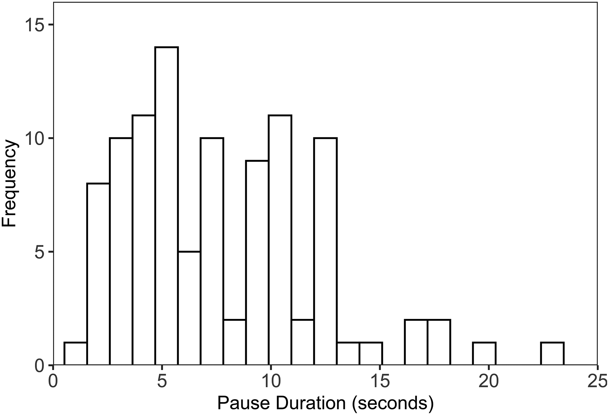
Histogram of children’s maximum pause durations in seconds.

Visualizing relationships between pause durations and continuous versus binned age.

Next we visualize the relationship between child age and pause duration in two ways, using a scatterplot of the relationship between continuous age (recorded as years to two decimal points; Figure 2A) and with a boxplot of the pauses with age-rounded age categories (Figure 2B). In both panels there appear to be slight, positive linear relationships between pause duration and age, such that older children tended to have longer maximum pauses. In fact, there is a significant positive correlation, r(99) = .26 [.06, .43], p = .010. However, this relationship is more difficult to observe from the box plot with rounded ages. Furthermore, the correlation for the relationship between rounded age and maximum pause is attenuated (27% smaller) and not significant, r(99) = .19 [−.01, .37], p =.060.

Figure 2.

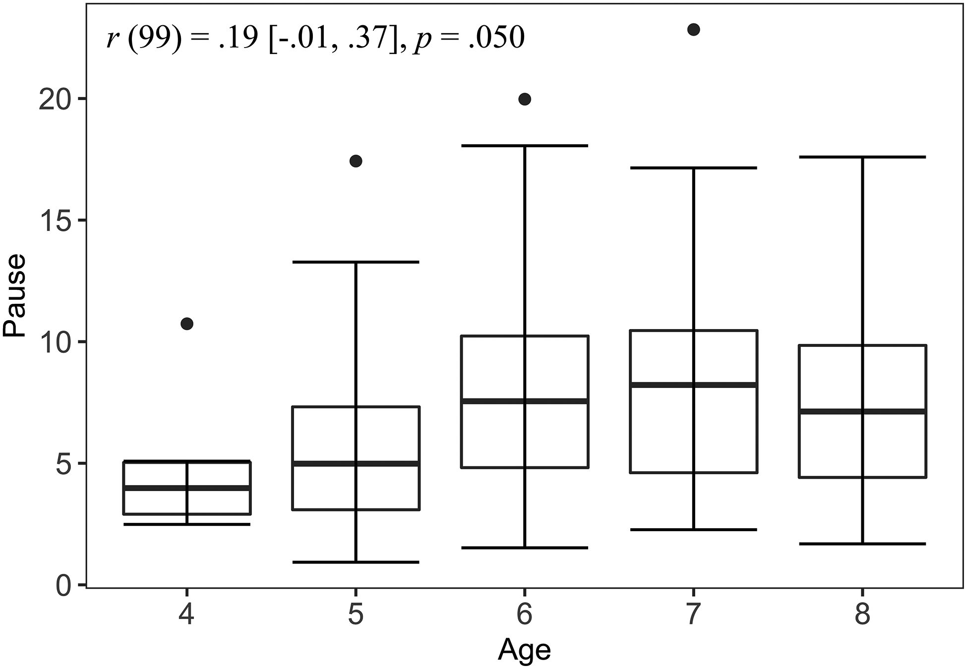
Top panel (A): relationship between continuous age in years and pause duration in seconds. Bottom panel (B): relationship between rounded age and pause duration.

Figure 2A also demonstrates how rounding age into categories obscures information about individual differences. The children identified with the square and diamond shapes receive the same value for age after rounding, whereas the children with the diamond and triangle shapes receive different values for age, despite the square and diamond shapes being farther from each other than the diamond and triangle shapes. Finally, we look at a scatter plot of pause duration by age and interview condition (Figure 3). The line of best fit for each experimental condition is also shown. This plot does not appear to show a main effect of interview condition or a markedly different relationship between age and pause duration across conditions. While the relationship between age and pause length appears to be fairly linear, the plots suggest the possibility of a quadratic trend, which we will also consider.

Figure 3.

Relationship between continuous age in years and pause duration in seconds in each experimental condition.

Testing for main effects and the interaction.

To formally test for possible age and interview effects and their interaction, researchers typically use either an ANOVA or a regression model. Although both traditional ANOVA and regression models are special cases of the general linear model, an important difference is that age is treated as a categorical variable in ANOVA and typically treated as a continuous predictor in regression. A long-standing misconception is that ANOVA is used for categorical predictors and regression is appropriate for continuous predictors when, in fact, any combination of categorical and continuous predictors is easily incorporated into a GLM analysis. (See the online supplemental file for a walk-through of this analysis using both SPSS and R) We recommend Judd, McClelland, and Ryan (2017) for an introductory text covering ANOVA and regression models in a unified GLM framework.

In Table 2 we present results side-by-side for our example data using the ANOVA model with categorical age (left panel) and a GLM framework with continuous age (right panel). The top panel includes models with main effects only. The summary table for the ANOVA model with categorical age indicates nonsignificant main effects of age, F(4, 95) = 1.59, p = .184 and interview condition, F(1, 95) = 2.86, p = .134¹. A significant main effect of age using ANOVA would show that mean pause duration differs across age categories, as depicted in Figure 2b. Treating age as a continuous predictor, even using rounded age, is used to test whether there is a non-zero expected increase in mean pause duration associated with each one year increase in age, and this relationship is significant in the GLM model, F(1, 98) = 7.41, p = .008. Note that the test for an age effect in the ANOVA model uses 4 degrees of freedom because the test is comparing means across 5 age categories (df = k-1, where k is the number of groups), whereas the GLM model tests the linear relationship between age and pause duration using 1 degree of freedom. Testing for mean differences among all age categories is less parsimonious and also more likely to overfit the data, capitalizing on chance differences among the means. Therefore, modeling the relationship between continuous (rather than categorical) age and pause duration is more appropriate for analyzing developmental trends and more powerful, in this case using only 1 degree of freedom to model a linear trend. We also tested a non-linear, quadratic age trend in our GLM model. This term was nonsignificant (b = −0.45, SE = 0.28, p = .093) and was dropped, confirming a linear relationship was adequate.

Table 2.

Traditional ANOVA and GLM Models of Pause Duration in Seconds by Age in Years and Experimental Condition

	Main effects only
	ANOVA model (categorical age)						GLM model (continuous age)
Summary table							Summary table
Predictor	SS	df	MS	F	p	${\eta }_{\text{p}}^2$ [95% CI]	SS	df	MS	F	p	${\eta }_{\text{p}}^2$ [95% CI]
Age	123.75	4	30.94	1.59	.184	.06 [.00, .14]	138.98	1	138.98	7.41	.008	.07 [.01, .18]
Condition	44.57	1	44.57	2.86	.134	.02 [.00, .11]	48.51	1	48.51	2.59	.111	.03 [.00, .11]
Error	1852.83	95	19.50				1837.59	98	18.75
							Parameter estimates
								b	[95% CI]	SE	t	p
							Intercept	6.73	[5.52, 7.94]	0.60	11.07	< .001
							Age	1.02	[0.28, 1.76]	0.37	2.72	.008
							Condition	1.39	[−0.32, 3.10]	0.86	1.61	.111
	Main effects with interaction
	ANOVA model (categorical age)						GLM model (continuous age)
Summary table							Summary table
Predictor	SS	df	MS	F	p	${\eta }_{\text{p}}^2$ [95% CI]	SS	df	MS	F	p	${\eta }_{\text{p}}^2$ [95% CI]
Age	122.82	4	30.70	1.54	.197	.06 [.00, .14]	138.79	1	138.79	7.33	.008	.07 [.01, .18]
Condition	51.69	1	51.69	2.59	.111	.03 [.00, .12]	47.60	1	47.60	2.51	.116	.03 [.00, .11]
Interaction	38.94	4	9.74	0.49	.744	.02 [.00, .06]	1.21	1	1.21	0.06	.801	< .01 [.00, .04]
Error	1813.88	91	19.93				1836.38	97	18.93
							Parameter estimates
								b	[95% CI]	SE	t	p
							Intercept	6.74	[0.91, 7.47]	0.61	11.01	< .001
							Age	0.92	[−0.14, 1.98]	0.53	1.73	.087
							Condition	1.38	[−0.35, 3.10]	0.87	1.59	.116
							Interaction	0.19	[−1.30, 1.68]	0.75	0.25	.801

Note. F tests for model effects are based on Type III SS for all models. Age was centered by subtracting the mean age from all ages to facilitate interpretation. Condition is coded 0 = control, 1 = experimental.

Whereas ANOVA tests of main effects are usually followed up by comparing pairs of means, for the GLM model similar tests are provided by the parameter estimates (i.e., regression coefficients) that define the model for our dependent variable, as shown for the GLM model in Table 2 and in equation 1. However, the way predictors are coded is important for interpreting these parameter estimates.

$${\text{Pause}}_i=b_0+b_1{\text{Condition}}_i+b_2{\text{Age}}_i+{\epsilon }_i$$ (1)

Specifically, interview condition is included as a binary dummy variable (0 = control condition, 1 = experimental condition), and this coding sets the reference category as the control condition. If we had more conditions, we could include additional dummy variables to compare among conditions (k-1, where k is the number of groups). We also subtract the mean age in the sample from observed ages, so the resulting intercept (b = 6.73, SE = 0.60, p < .001) is interpretable as the predicted pause for a child whose age is equal to the mean age of the sample (M = 6.76) in the control condition (i.e., when all predictors are zero). The coefficient for the effect of age shows that pauses tend to be about 1 second longer for each year increase in age (b = 1.02, SE = 0.37, p = .008). The coefficient for condition (b = 1.39, SE = 0.86, p = .111) indicates that pauses in the experimental condition tended to be 1.39 seconds longer but that this difference between conditions was not significant.

The second set of models in the lower half of Table 2 show that the interaction between condition and age is not significant in either model. Notice that the interaction effect for the ANOVA model with categorical age uses 4 degrees of freedom, and this is in order to test for differences in the patterns of mean differences; i.e., does the effect of condition differ across age categories? This interaction test is considerably less parsimonious than the test in the GLM model, where age is treated as a continuous predictor.

Although not significant, the coefficient for the interaction in the GLM model is interpreted as the difference in slopes relating age and pause duration, and that relationship was stronger in the experimental condition (b = 0.92 in the control condition; slope = 0.92 + 0.19 = 1.11 in the experimental condition). Unlike ANOVA, in the GLM model, the coding of predictors determines how the effects of predictors are interpreted when an interaction effect is included. In this case, with child age centered at the sample mean, the parameter estimate associated with the effect of condition (0 = control, 1 = experimental) represents the expected effect of the experimental condition (relative to control) for a child of average age in the sample. However, because condition is dummy coded with the control group as the reference, the effect of age is interpreted as the expected increase in pause length per one year increase in age for children in the control condition. Because the results and examination of the data show no evidence of an interaction effect, the interaction term could be omitted, and we return to the GLM model with main effects only, where the overall effect of age on pause duration is significant.

Summary of conclusions from the real data example.

Relating back to the original research question, these results show that pauses that are longer than what is typical of adult dialogue are important to give children time to respond, as discussed by Rezmer et al. (2020). The predicted (average) maximum pause duration for each age can be obtained using the model equation (e.g., for children age 4 in the control condition: pause = 6.74 + 1.02*[4 – 6.76] = 3.92 seconds); however, because some children had maximum pauses outside of this range, the practical implication of these results is that longer interviewer wait times are recommended when interviewing children. A single wait time could be recommended, regardless of the child’s age, or the recommended wait time could be tailored to fit the predicted range for specific ages.

This example highlights the importance of appropriately analyzing developmental trends. Binning age in this case would have led to the inappropriate conclusion that child age is unrelated to pause duration. Besides this, in the next section we illustrate additional incorrect inferences that may be made as a result of binning.

Simulated Example

In our example data, binning age led to less power to detect significant effects, but this will not always be the case. Because binning introduces measurement error, sometimes binning produces significant effects when the continuous version does not. To demonstrate this, we present results from a simulated example based loosely on our real data where we have included a continuous covariate, language ability, that is correlated with age but has no effect on pause length (i.e. the partial correlation between language ability and pause length is zero). Specifically, age and language are drawn from a bivariate normal population and correlated r = .80, and the regression equation for pause is

$$\begin{gathered} {\text{Pause}}_i=6.00+1.50\times {\text{Age}}_i+0\times {\text{Language}}_i+{\epsilon }_{i,} \\ \text{var}\left({\epsilon }_i\right)=1.69 \end{gathered}$$ (2)

These parameters correspond to a strong positive relationship between age and pause duration (${\eta }_{\text{p}}^2$ = .32), a strong positive correlation between age and language ability, but the true effect of language ability on pause length is zero with no interaction effect. This (fictitious) model would suggest that pause length is a developmental process unrelated to language ability. Full code for the simulation and analyses is available in the supplemental material.

We simulated 10,000 data sets of n = 100 each from this model, and for each data set we ran the analysis 2 ways: (1) GLM/regression (continuous age) and (2) ANOVA splitting both age and language ability at their medians (i.e. categories for “younger” and “older” children as well as “low” and “high” language ability). For each analysis, we simultaneously tested the main effect of age, language, and the interaction.

The results across data sets are summarized in Table 3. For the model with age treated continuously, the results are unsurprising: the effect of age is significant in 100% of the replications for this sample size. The effect of language and the interaction effect, which are truly zero, are significant 5% of the time, in line with α = .05. However, the effect of language emerges as significant 27% of the time when the predictors were binned into categories at the median. We also see that the effect size for age is greatly underestimated when age is treated as a dichotomous predictor.

Table 3.

Results of Significance Tests for Age and Language Ability From 10,000 Simulated Replications with n=100.

		ANOVA model		GLM model
Predictor	True ${\eta }_{\text{p}}^2$	(dichotomous age)		(continuous age)
		Obs. ${\eta }_{\text{p}}^2$	% Sig	Obs. ${\eta }_{\text{p}}^2$	% Sig
Age	.34	.12	94	.33	100
Language	0	.03	27	.01	5
Interaction	0	.01	4	.01	5

Note. Obs. ${\eta }_{\text{p}}^2$ is the observed value of ${\eta }_{\text{p}}^2$ effect size. Significance values for predictors are from F tests using Type III SS.

Why does the main effect of language now appear significant when the true effect is zero? In this example, the misspecification created by binning or dichotomizing age and language results in a biased and spurious effect of language. Although binning most often results in attenuated power, inflated Type I error rates such as in this example may also occur depending on the pattern of correlations among the predictors and outcome variable, as described in detail in several methodological articles (MacCallum et al., 2002, Maxwell & Delaney, 1993, Vargha et al., 1996). When two predictors are correlated and the partial correlation of one predictor with the outcome variable is near zero, as in our example, Type I error rates are likely to be inflated. Other misspecifications, such as unmodeled nonlinearity in the effects of one or more predictors, may also lead to spurious interaction effects (Maxwell & Delaney, 1993). Treating age and language as continuous predictors properly accounts for the true relationships present in the data, telling the whole story, whereas binning into categories leads to misleading results.

In our real data and simulated examples, the data were relatively well-behaved. A number of additional complications may arise, however. One concern is whether the relationship between age and the dependent variable is in fact linear. A researcher may wish to bin age in order to avoid assuming a linear relationship between age and the outcome, although this would still be unwarranted. First, inspection of the relationship between the actual data, as in Figure 2A, is crucial for detecting potential nonlinear relationships. Rather than throw away information about individual age differences, a notably nonlinear relationship can be appropriately modeled using quadratic and even cubic polynomial terms, transformations, or nonlinear models. Another frequent concern is non-normal residuals. As we noted earlier, unless the distribution is extremely non-normal (for example, the distribution is categorical or extremely skewed), results are robust for the sample sizes and distributions common in eyewitness testimony research. General rules of thumb about required sample size are woefully imprecise because the size needed depends on the number of predictors and the extent of non-normality of the errors; for example, N > 100 is necessary for an extremely skewed error distribution (skew = 7), but with moderate nonnormality (skew = 1) performance is satisfactory with N = 5 (see Pek, Wong, & Wong, 2018, for in-depth treatment and examples).

To summarize, binning age in an analysis sacrifices information, reduces power, attenuates relationships, introduces error, and may lead to spurious effects. Instead of binning age in order to use age as a variable in an ANOVA framework, a general linear model framework can be used to flexibly test for effects of combinations of continuous and categorical predictors, including interactions. The resulting models convey a more complete story of developmental trends—a story that better mirrors what we are able to visualize using descriptive plots.

This approach to developmental data, which involves inspecting distributions and selecting the analytical strategy most likely to capture the observed trends, should not be overruled by a priori categories reflecting the age associated with a developmental achievement or legally-defined transition, such as age when juveniles are first treated as adults. Although the law must necessarily draw lines that separate younger from older individuals, statistical comparisons of these groups do not reveal whether those lines are currently positioned where a developmental discontinuity occurs or, in the legal arena, where they will best achieve some socially-desired goal. For example, contrasting 14- to 16-year-olds and 17- to 19-year-olds returns a conclusion about the difference between group averages, but this says nothing about whether 17-year-olds are more like 16-year-olds or 18-year-olds. Analyzing age as a continuous variable improves our ability to detect a developmental change in this age range and accurately characterizes the effect size. Follow-up analyses can then determine the age (or ages) where meaningful change occurs.

Discussion

Because findings from child eyewitness studies have serious implications for child protection and social justice, it is important that researchers’ conclusions acknowledge and accurately describe developmental differences in eyewitness performance. Developmental studies are challenging to power, however, because it can be difficult—and costly—to enroll large numbers of children. Often, researchers obtain sufficient numbers of participants by enrolling children within a broad age range but including only a small number representing each year of age. Because findings from child eyewitness studies have serious implications for child protection and social justice, it is important that researchers’ conclusions acknowledge and accurately describe developmental differences in eyewitness performance. To minimize erroneous conclusions without increasing sample sizes, researchers interested in age effects must adopt statistical practices that maximize power to detect real differences without inflating the frequency of spurious results. This is easily accomplished by treating age as a continuous variable in a general linear model framework.

Colleagues have asked us why it is problematic to miss an age trend. Consider, for instance, an interviewing strategy that slightly improves young children’s testimonial accuracy but has a greater effect among older children. What harm does it do to recommend that strategy for all age groups? Our answer is that policy-making often involves decisions about competing strategies, interventions, or policies. Forensic interviewers, for instance, may have a window of time to interview each child, and that window can be shorter for young children due to their limited ability to stay on task. Consequently, forensic protocols do not include all procedures that improve children’s reports. Instead, policy-makers aim to populate protocols with practical (i.e., feasible in the field and trainable) techniques that provide the largest benefits, along with those that reduce serious (even if infrequent) errors. Understanding developmental trends and comparing effect sizes is crucial for selecting the most efficacious set of techniques for children of various ages. Insufficient attention to developmental trends leads to myriad problems, including interviewers who are scared to shorten the ground rules phase during conversations with very young witnesses and expert testimony that thoughtlessly generalizes preschoolers’ limitations to cases involving much older children.

Of course, the diversity of topics in psychology-law precludes dictating one statistical approach for all purposes. But for most developmental studies, recording age in months or in years to two decimal places (when possible), visually inspecting distributions and age trends, and treating age continuously in analyses will feed better information about age differences into decision-making about children and the law.

Public Significance Statement:

Researchers who study children’s eyewitness testimony frequently look for developmental trends by comparing children’s performance across discrete age groups. Statistical approaches that treat age as a continuous variable are more likely to return accurate conclusions about children’s strengths and weaknesses as witnesses, however, and should be the usual way of analyzing developmental trends. An online supplement illustrates this approach through example code and annotated output from SPSS and R.

References

- Bainter SA, Tibbe TD, Goodman ZT, & Poole DA (2020). Child eyewitness researchers often bin age: Prevalence of the practice and recommendations for analyzing developmental trends [Data set] Retrieved from www.osf.io/6w2sc [DOI] [PMC free article] [PubMed]
- Baker BA, Poole DA, & Dickinson JJ (2015, March). Sex differences in children’s suggestibility: Do they exist? Paper presented at the annual meeting of the American Psychology-Law Society, San Diego, CA, USA. [Google Scholar]
- Bruck M, & Ceci SJ (2012). Forensic developmental psychology in the courtroom In Faust D (Ed.), Coping with psychiatric and psychological testimony: Based on the original work by Jay Ziskin (pp. 723–736). New York, NY: Oxford University Press. doi: 10.1093/med:psych/9780195174113.003.0034 [DOI] [Google Scholar]
- DeCoster J, Gallucci M, & Iselin AR (2011). Best practices for using median splits, artificial categorization, and their continuous alternatives. Journal of Experimental Psychopathology, 2, 197–209. doi: 10.5127/jep.008310 [DOI] [Google Scholar]
- Dickinson JJ, & Poole DA (2017). The influence of disclosure history and body diagrams on children’s reports of inappropriate touching: Evidence from a new analog paradigm. Law & Human Behavior, 41, 1–12. doi: 10.1037/lhb0000208 [DOI] [PubMed] [Google Scholar]
- Field A, Miles J, & Field Z (2012). Discovering statistics using R. Thousand Oaks, CA: Sage. [Google Scholar]
- Hale GA (1977). On use of ANOVA in developmental research. Child Development, 48, 1101–1106. doi: 10.2307/1128369 [DOI] [Google Scholar]
- Judd CM, McClelland GH, & Ryan CS (2018). Data analysis: A model comparison approach to regression, ANOVA, and beyond. New York, NY: Routledge. [Google Scholar]
- Lamb ME, Brown DA, Hershkowitz I, Orbach I, & Esplin PW (2018). Tell me what happened: Questioning children about abuse (2nd ed.). Hoboken, NY: Wiley-Blackwell. doi: 10.1002/9781118881248 [DOI] [Google Scholar]
- Lumley T, Diehr P, Emerson S, & Chen L (2002). The importance of the normality assumption in large public health data sets. Annual Review of Public Health, 23, 151–169. doi: 10.1146/annurev.publhealth.23.100901.140546 [DOI] [PubMed] [Google Scholar]
- MacCallum RC, Zhang S, Preacher KJ, & Rucker DD (2002). On the practice of dichotomization of quantitative variables. Psychological Methods, 7, 19–40. doi: 10.1037/1082-989x.7.1.19 [DOI] [PubMed] [Google Scholar]
- Maxwell SE, & Delaney HD (1993). Bivariate median splits and spurious statistical significance. Psychological Bulletin, 113, 181–190. doi: 10.1037/0033-2909.113.1.181 [DOI] [Google Scholar]
- Maxwell SE, & Delaney HD (2004). Two-way between-subjects factorial designs In Designing Experiments and Analyzing Data: A Model Comparison Perspective (pp. 275–353). New York, NY: Taylor & Francis Group. [Google Scholar]
- Myers JEB (2016). Myers on evidence of interpersonal violence: Child maltreatment, intimate partner violence, rape, stalking, and elder abuse (6th ed.). New York, NY: Wolters Kluwer. [Google Scholar]
- Pek J, Wong O, & Wong ACM (2018). How to address non-normality: a taxonomy of approaches, reviewed, and illustrated. Frontiers in Psychology, 9, 1–17. doi: 10.3389/fpsyg.2018.02104 [DOI] [PMC free article] [PubMed] [Google Scholar]
- Poole DA, Brubacher SP, & Dickinson JJ (2015). Children as witnesses In Cutler BL & Zapf PA (Eds.), APA handbook of forensic psychology (Vol. 2, pp. 3–31). Washington, DC: American Psychological Association. [Google Scholar]
- Rezmer B, Trager LA, Catlin C, & Poole D (2020). Pause for effect: A 10-second interviewer wait time gives children time to respond to open-ended prompts. Journal of Experimental Child Psychology, 194, 1–9. doi: 10.1016/j.jecp.2020.104824 [DOI] [PubMed] [Google Scholar]
- Vargha A, Rudas T, Delaney HD, & Maxwell SE (1996). Dichotomization, partial correlation, and conditional independence. Journal of Educational and Behavioral Statistics, 21, 264–282. doi: 10.2307/1165272 [DOI] [Google Scholar]
Associated Data
This section collects any data citations, data availability statements, or supplementary materials included in this article.