

Abstract
Geometric morphometrics is the statistical analysis of landmark-based shape variation and its covariation with other variables. Over the past two decades, the gold standard of landmark data acquisition has been manual detection by a single observer. This approach has proven accurate and reliable in small-scale investigations. However, big data initiatives are increasingly common in biology and morphometrics. This requires fast, automated, and standardized data collection. We combine techniques from image registration, geometric morphometrics, and deep learning to automate and optimize anatomical landmark detection. We test our method on high-resolution, micro-computed tomography images of adult mouse skulls. To ensure generalizability, we use a morphologically diverse sample and implement fundamentally different deformable registration algorithms. Compared to landmarks derived from conventional image registration workflows, our optimized landmark data show up to a 39.1% reduction in average coordinate error and a 36.7% reduction in total distribution error. In addition, our landmark optimization produces estimates of the sample mean shape and variance-covariance structure that are statistically indistinguishable from expert manual estimates. For biological imaging datasets and morphometric research questions, our approach can eliminate the time and subjectivity of manual landmark detection whilst retaining the biological integrity of these expert annotations.
Keywords: Anatomical landmark, deep learning, geometry, image registration, micro-computed tomography, morphometrics
Introduction
Anatomical landmarks are central to geometric morphometrics (GM) and the study of shape variation. Landmarks are Cartesian coordinate points in two or three dimensions that are homologous across samples (Bookstein 1991). Taken together, a landmark configuration represents the shape and size of an object in a statistically tractable manner, allowing for tests involving multiple covariates and/or factors, as well as intuitive visualizations of variation (Adams et al. 2004, 2013; Mitteroecker and Gunz 2009). The gold standard approach to landmark acquisition is manual detection by a single observer on all individuals within a single study (Zelditch et al. 2012). While this approach is feasible for small studies, it is not scalable to large datasets, and landmark data collected across multiple studies cannot be easily combined for larger-scale analyses (Hallgrímsson et al. 2009a). Big data approaches, such as deep phenotyping (Bycroft et al. 2018; Robinson 2012) and phenomics (Freimer and Sabatti 2003; Houle et al. 2010; Schork 1998), require morphological data collection to be rapid, precise, and consistent across large and complex imaging datasets. In this paper, we combine techniques from image registration, GM, and machine learning to automatically and accurately detect anatomical landmarks.
Image registration refers to the spatial alignment of images and is a fundamental task in biological image analysis (Oliveira and Tavares 2014). To achieve spatial normalization, registration methods involve an initial affine transformation for global alignment, followed by a deformable transformation for non-linear alignment. After establishing spatial correspondences at every voxel, a set of labels (e.g., landmarks or segmentations) can be propagated from one image to the other. An atlas is often used for pairwise registration, because it represents a labelled population average that best minimizes differences from the rest of the sample (Evans et al. 2012; Friedel et al. 2014; Maga et al. 2017; Mazziotta et al. 2001). Registration methods are well-suited for GM and phenomics, because they ensure a common shape space (Dryden and Mardia 1998; Raup 1966) for homologous landmark detection and biological data integration (Hallgrímsson et al. 2009b; Klingenberg 2002). In addition, the use of an atlas encourages data standardization. As morphological datasets become increasingly large and accessible, it is important they be relatable through a shared set of labels.
While registration-derived landmarks are appealing for biology and morphometrics, among other disciplines, their anatomical precision depends on the integrity of the deformable registration (Sotiras et al. 2013). Unfortunately, as a complex optimization problem, it is not uncommon to converge on a deformable registration solution that yields suboptimal non-linear displacements around morphological extrema. High morphological variation at these points leads to interpolation artifacts, improper regularization, and/or violation of the one-to-one correspondence assumption in registration (Heckemann et al. 2006). This misalignment results in labelling errors. To minimize such error, it is common to employ some form of (multi-atlas) label fusion (Wang et al. 2012). For example, Bromiley et al. (2014) non-linearly registered image patches from a training database to a specimen image and combined the propagated landmarks with an array-based voting scheme. Young and Maga (2015) utilized another voting mechanism called shape-based averaging (Rohlfing and Maurer 2007) to fuse landmarks detected via single and multi-atlas (Wang et al. 2012) approaches. These approaches, however, require multiple non-linear registrations per specimen and still produce landmark configurations that are statistically distinguishable from manual annotations. Percival et al. (2019) show that these landmark detection errors can produce misleading representations of the mean shape, an underestimation of biological signal, and altered variance-covariance patterns
We present an approach that combines image registration, GM, and deep learning to automatically and accurately detect landmarks. To initially detect the landmarks, we implement two fundamentally different deformable registration algorithms: ANIMAL (Automatic Nonlinear Image Matching and Anatomical Labelling) (Collins and Evans 1997) and SyN (Symmetric Normalization) (Avants et al. 2011). After registration, we optimize landmark detection by applying a feedforward neural network (FFNN) with a domain-specific loss function. The network learns a multi-output regression model that minimizes automated and manual shape differences. We validate our framework and landmark results in a morphologically diverse sample of adult mouse skull images acquired via micro-computed tomography (μCT). Our validation focuses on the ability of optimized automated landmarks to improve (a) individual and mean representations of shape, (b) sample-wide distance relationships, and (c) variance-covariance patterns. Because our approach relies exclusively on image intensities and shape coordinates, it is generalizable to other volumetric imaging modalities, anatomy, and landmark configurations.
Methods
Image acquisition and manual landmarks
We construct a database of adult mouse skull μCT images (N=4805) representing 216 strain/genotype groups derived from various studies of craniofacial variation (e.g., Attanasio et al. 2014; Hallgrímsson et al. 2004, 2006, 2009; Lieberman et al. 2008). The genetic groups include 120 wild-derived and common laboratory inbred strains, as well as 96 experimental strains (heterozygous or homozygous for a genetic mutation). All μCT volumes were obtained in the 3-D Morphometrics Centre at the University of Calgary using a Scanco vivaCT40 scanner (Scanco Medical, Bruttisellen, Switzerland) with 0.035 × 0.035 × 0.035 mm3 spatial resolution, 55 kV, and 72–145 μA. The same p × k landmark configuration containing p = 68 landmarks in k = 3 dimensions (Fig. 1) was manually recorded for all specimens by a single expert observer using minimum threshold-defined bone surfaces in Analyze (www.mayo.edu/bir/).
Fig. 1:
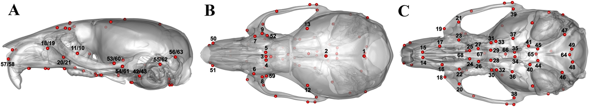
Standard skull landmark configuration on a mesh of the global reference atlas with (A) lateral, (B) superior, and (C) inferior views.
Atlas construction
An atlas is a population average constructed via iterative alignment and averaging, either using the sample images themselves or an external dataset. We use the available database images and manual landmark data to identify a comprehensive set of genetic groups for atlas construction. We superimpose the manual landmark configurations into a common shape space via Generalized Procrustes Analysis (GPA) (Gower 1975; Rohlf and Slice 1990). We compute the mean shape for each genetic group and subject these means to a principal component analysis (PCA). We extract all images (n = 529) from a subset of genetic groups with mean shapes at the extremes of the first five principal components (PCs), as well as one close to the grand mean (Fig. S1). To perform the superimpositions and PCA sampling, we use the Morpho (Schlager 2017) and base stats packages in R (R Core Team 2018). We feed the entire image sample into a group-wise registration pipeline (Appendix S1) to construct a single global reference atlas. Both the atlas and our standard landmark configuration are shown in Fig. 1.
Training and test set images
A high amount of morphological variation is needed to test the generalizability of a registration and learning-based workflow. We randomly sample a single image from each genetic group across the database (n = 216) to generate a morphologically diverse sample for training and testing our neural networks. We verify the extent of this subsample morphospace by ensuring their Procrustes distances to the grand mean shape is equivalent to that of the entire database. Using a density permutation (nperm = 999) test in the sm package (Bowman and Azzalini 2018), we observe that both distributions are statistically indistinguishable at a significance level of α = 0.05 (Fig. S2). We split the image sample into training (n = 170) and test (n = 46) sets in preparation for deformable registration and neural network shape optimization. Prior to running deformable registration, we affine align every volume to our atlas (Appendix S1)) and store the scaling and shear factors, leaving only non-linear differences as a source of misalignment.
Deformable registration and landmark propagation
Deformable registration may be performed with large and small deformation algorithms. While large deformation approaches optimize non-linear displacements jointly across the entire registration field, small deformation approaches emphasize local optimization of displacements. We implement the geodesic SyN (large deformation) and ANIMAL (small deformation) algorithms to pairwise register each image to the atlas, because they are fundamentally different and thus allow us to evaluate the generality of our approach. Geodesic SyN computes a non-linear correspondence map between the image pair by integrating a velocity field, or a vector field that updates through time. This registration is considered symmetric in that it defines a variational energy splitting the spatial normalization in half. Each volume contributes equally to the geodesic, or shortest, path and deformation between them. ANIMAL generates a non-linear correspondence map in a piecewise manner using local deformation lattices. Displacement vectors at each node in the lattice are estimated independently via local 3-D simplex optimization (Nelder and Mead 1965) and are built up to produce a full deformation field. We optimize the parameters of SyN and ANIMAL using a cross-correlation objective function to keep the similarity metric constant. We recover the non-linear transformations, concatenate them with our affine transformations, and propagate the atlas landmarks along this path to the rigid space of each image (Fig. 2A).
Fig. 2:
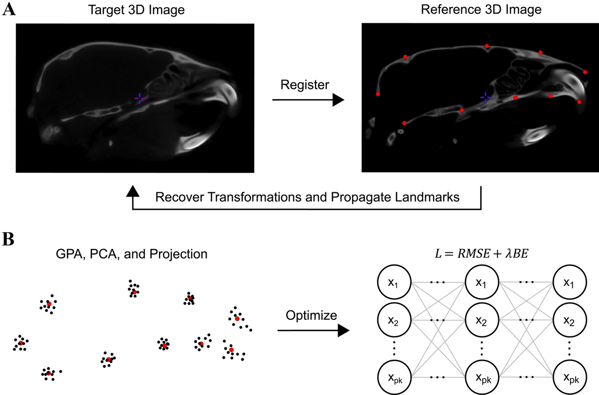
Schematic overview of the workflow. (A) We non-linearly deform an input image to the reference atlas image, recover the transformation, and propagate the landmarks along this path. (B) We superimpose the training and test landmarks onto the sample mean shape, then project them into a linear tangent space. After training the FFNN to minimize a root mean squared error (RMSE) and bending energy (BE) loss function, we apply the network to the test tangent space coordinates to optimize their detection.
Neural network shape optimization
Misdetection of only a few landmarks via local non-linear displacement error can lead to improper representations of shape (Percival et al. 2019). We formulate registration-based landmark detection as a supervised deep learning task to minimize this error and thus improve GM analyses. To ensure our landmark data are in the same shape space for training and testing, we compute the mean shape of the manual training data and GPA all automated configurations to this mean. We orthogonally project the Procrustes aligned configurations into the tangent space of the manual mean to leverage the statistical properties of Kendall’s tangent space coordinates (Kendall 1984), otherwise known as Procrustes shape variables (Fig. 2B). This projection linearizes the data and simplifies the problem of learning non-linear shape differences at each point. In addition, the range of Procrustes shape variables ensures that each landmark contributes proportionately to the loss function, and that the optimizer (e.g., gradient descent) converges faster.
For each deformable registration workflow, we train a deep FFNN to learn a multi-output regression model that minimizes automated and manual shape differences (Fig. 2B). The network contains an input layer, three hidden layers, and an output layer. We define p × k fully connected neurons in each layer to integrate across the entire configuration and therefore consider covariance among landmarks. Rectified linear unit activations are used in the hidden layers and identity activations in the output layer. With the Adam optimizer (Kingma and Ba 2015) and a learning rate of 0.01, we train the networks over 10000 epochs to minimize a domain-specific loss function, L = RMSE + λBE, where RMSE is root mean squared error, BE is bending energy, and λ is a stiffness coefficient empirically determined to be 0.001. If we let xℓ(T) and denote the observed and predicted vectors at landmark ℓ for a given specimen T, RMSE takes the form of Procrustes distance:
While minimizing RMSE will encourage configurations to better distribute about the mean, it may also encourage non-smooth transformations. We add a thin-plate spline BE term (Bookstein 1989; Duchon 1976; Rueckert et al. 1999) to regularize the landmark displacements. If W is a mapping from to for a given specimen T, the mean BE is expressed as
We train all models on an NVIDIA GeForce GTX 1080 Ti in Julia (Bezanson et al. 2017) using the Flux machine learning library (Innes 2018). After training, we evaluate each network on the test Procrustes shape variables and compare the predictions with their manual counterparts via standard GM analyses. To simplify the analyses below, we use the term “workflow” to refer to our test groups: SyN, ANIMAL, SyN-Opt, and ANIMAL-Opt.
Landmark-by-landmark error comparisons
Shape is a combination of landmark distances and angles. To examine landmark-by-landmark detection errors for each workflow, we consider both the magnitude of difference and the distribution of deviations around each landmark (O’Higgins et al. 2001; von Cramon-Taubadel et al. 2007). We calculate the automated-manual Euclidean distance at each landmark for every specimen as a linear measure of error magnitude. We refer to these distances as “relative linear errors” to emphasize that these locally Euclidean displacements are relative to one another and are not independent. In almost all analyses below, we multiply these shape measurements by the original specimen centroid sizes to interpret error on the scale of millimeters.
Since our manual landmarks were acquired over a period of 15 years, we had to account for manual detection drift. We subtract the mean manual intra-observer error magnitudes reported in our previous work (Percival et al. 2019) from the conventional relative linear errors to arrive at a conservative estimate of registration-based landmark error. Conventional automated landmarks with errors exceeding 0.25 mm (seven voxel lengths) are defined as problematic, because it has been shown that intra-observer error at most landmark points across the mouse skull tends to be 0.25 mm or less (Percival et al. 2014). For reference, the size of an average wild type mouse skull is approximately 10 mm in width, 6 mm in height, and 22 mm in length (Vora et al. 2016).
Given the repeated observations across our datasets, we estimate the effects of workflow on relative linear error with a mixed-effects model using specimen index as a random effect. We implement the models with the lme4 package (Bates et al. 2015). We sum the squared relative linear errors across all landmarks to compute a density of intra-specimen distances. To quantify differences in the distribution of automated and manual landmarks, we generate a covariance matrix for every landmark and compute an automated-manual Procrustes shape metric for covariance distance (Dryden et al. 2009; Dryden 2018). A covariance distance of 0 indicates that the automated and manual landmark distributions are equivalent.
Landmark configuration comparisons
Sample-wide distance relationships are evaluated using entire landmark configurations. We assess overall configuration error by computing the RMSE between automated and manual configurations. We subject these RMSE values to a two-way ANOVA to reveal whether a particular workflow exhibits a statistically significant reduction in average error. We also regress RMSE on Euclidean distance to the manual mean shape to test the hypothesis that increasingly extreme morphology correlates with registration error. To understand how configurations position themselves in space relative to the gold standard mean, we calculate manual distances to the mean and compare their distribution with the automated distances.
Automation generally suppresses the variance in a sample by reducing measurement error and underestimating biological signal (Li et al. 2017; Percival et al. 2019). We perform a multivariate ANOVA (MANOVA) with the RRPP package (Collyer and Adams 2018, 2019) to test whether the automated workflows reproduce the manual mean shape. Using the superimposed configurations as the dependent variable and workflow as the sole predictor, this MANOVA fits a least squares model over random permutations (nperm = 999) of landmark data to generate an empirical sampling distribution for significance testing. We subject the MANOVA fitted values to a PCA and extract post-hoc automated-manual shape distances and landmark vector correlations among mean shapes. To visualize automated and manual mean shape differences, we produce a surface mesh of the atlas and deform it to each mean by way of thin-plate spline. We use the Morpho package to show mean automated-manual distances at every vertex of the deformed meshes.
To analyze automated-manual similarity across the major axes of covariance, we decompose each covariance matrix of Procrustes shape variables into PCs. Direct PC comparisons are made by projecting the automated configurations into the manual PC space. We retain a sense of mean differences by correlating the uncentered manual and automated PC scores with the corrplot package (Wei and Simko 2017). Visualizations of the sample distribution along the first several PCs is simplified by computing convex hulls with the vegan package (Oksanen et al. 2019). In addition, we calculate and resample (nresample = 999) the trace of each covariance matrix to compare sample variances. For a more granular understanding of where automation suppresses this variance, we perform a relative eigenanalysis (Bookstein and Mitteroecker 2014) using the vcvComp package (Le Maîitre and Mitteroecker 2019).
Results
The majority of landmarks were well detected by both conventional registration workflows. We found that problematic landmarks tend to reside in the same areas of the skull. After adjusting for mean intra-observer landmark drift, landmarks 2, 7, 12–13, 48–52, and 68 exceeded the problematic 0.25 mm threshold for SyN (Fig. 3A,C and Table S1). Landmarks 2, 7, 10–13, 48–52, and 68 failed for ANIMAL (Fig. 3A,C and Table S1). Thus, most problematic landmarks are problematic for both deformable registration workflows. Landmarks 2 and 7 define the bregma and anterior-most point along the lateral zygomatic-frontal suture, respectively. Landmarks 12–13 reside near the apex of the cranial vault at the frontal-temporal-parietal junction. Landmarks 48–49 are located at the posterior point of the basioccipital. Landmarks 50–51 occupy the anterior point of the nasal-premaxilla suture. Landmark 68 is a midline endocranial point that represents the intersection of the frontal bones and the anterior-most point of the cribriform plate of the ethmoid. Taken together, these problematic landmarks represent some of the most extreme superior, anterior, and posterior-inferior points of the skull. Mean relative linear error at these landmarks ranged between 0.26 mm and 0.52 mm (Table S1). The only markers not classified as problematic in both unoptimized workflows were landmarks 10 and 11, which exhibited mean relative linear errors of 0.26 mm and 0.27 mm, respectively (Table S1).
Fig. 3:
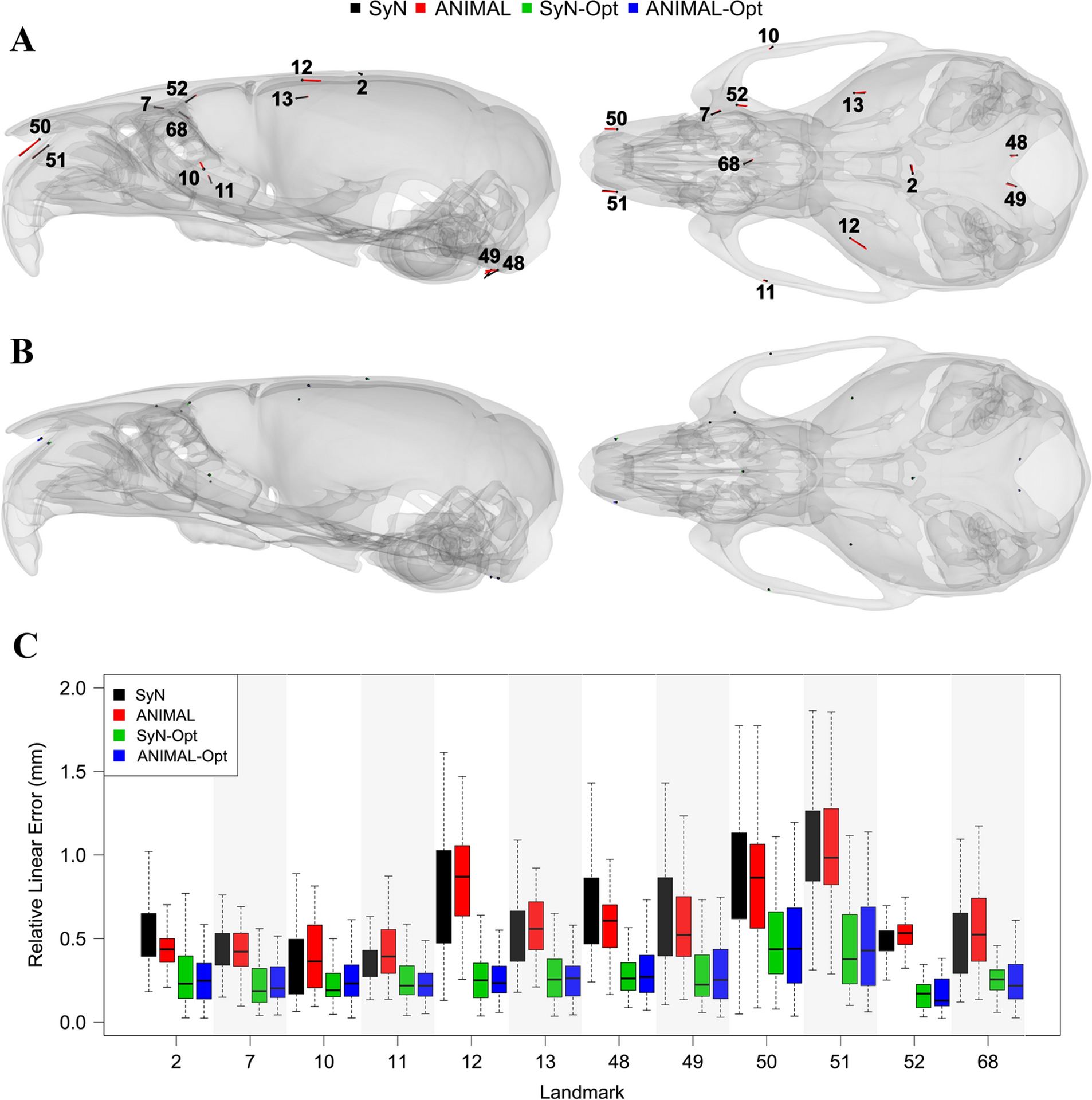
Visualization of problematic landmarks that showed ≥ 0.25 mm of automated error relative to the manual landmarks, with lateral (left) and superior (right) skull views. Observe that the mean (unscaled) landmark error magnitudes for the (A) conventional workflows are large and directionally consistent in an unoptimized state, yet barely discernible after (B) optimization. (C) Relative linear errors for the problematic automated landmarks.
Optimization reduced the mean relative linear error for the majority of conventional registration landmarks, including for all problematic landmarks (Fig. 3B,C and Table S1). SyN optimized, or SyN-Opt, yielded reductions in mean relative linear error at 59 of the 68 landmarks. This reduction ranged between 0.004 mm and 0.60 mm. Interestingly, small yet notable error increases of 0.04 mm were seen at landmarks 8 and 9. ANIMAL optimized, or ANIMAL-Opt, largely recapitulated what was observed with SyN-Opt. Error reductions between 0.004 mm and 0.58 mm were observed at 58 of the 68 landmarks. In addition, a small but notable error increase of 0.03 mm was detected at landmark 37.
The average automated-manual landmark deviation, or RMSE, across all optimized configurations was significantly lower than what was seen in the conventional registration-based configurations (Fig. 4A). While the conventional SyN and ANIMAL workflows exhibited an average RMSE of 0.23 mm, their optimized counterparts, SyN-Opt and ANIMAL-Opt, both showed statistically significant (p < 0.0001) RMSE reductions of 0.09 mm (39.1%). Interestingly, even with smaller training datasets of n=50 and n=100, the optimized configurations showed significant average RMSE reductions of 0.07 mm (30.4%, p < 0.0001) and 0.05 mm (21.7%, p < 0.0001), respectively (Fig. S3).
Fig. 4:
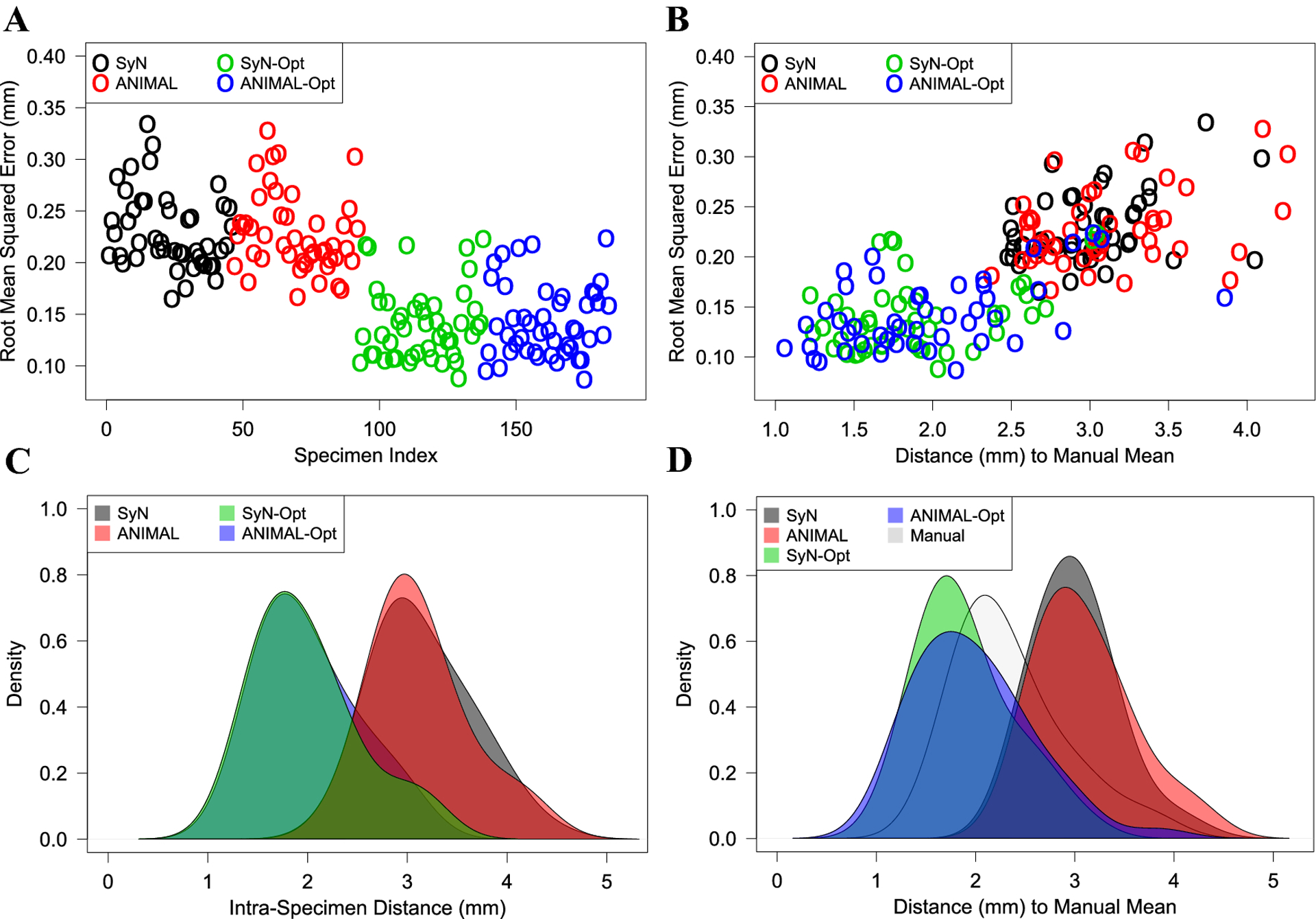
(A) Average landmark deviation, or RMSE, between each automated configuration and their corresponding manual configuration. (B) Relationship between RMSE and distance to the manual mean shape. (C) Density of distances between corresponding automated and manual configurations. (D) Comparison of automated distances to the manual mean shape relative to the true manual distances.
We observed that increasingly dysmorphic skull shapes, or those positioned further from the manual mean shape, did not necessarily exhibit higher landmark error. Among workflows RMSE increased by 0.043 mm (r = 0.75, p < 0.0001) for every standard deviation (0.74 mm) from the mean shape. However, the relationship between RMSE and distance is fairly weak within workflows (Fig. 4B), suggesting that detection error, rather than increasingly dysmorphic anatomy, perturbs distance relationships relative to the mean shape.
Aggregating relative linear errors over corresponding configurations, the mean intra-specimen Euclidean distances were, from greatest to least, ordered as follows: SyN-Opt, ANIMAL-Opt, ANIMAL, SyN (Fig. 4C). The mean intra-specimen Euclidean distance for optimized methods was 2.0 mm, whereas the unoptimized mean distance was 3.1 mm. Upon evaluating distance relationships relative to the mean shape, the optimized distributions were more similar to the manual distribution than were unoptimized distributions (Fig. 4D). The ability of optimization to improve distance relationships across the sample is further shown in Table 2, where distance quantiles for each workflow are enumerated.
Table 2.
Summary statistics of automated and manual distances (mm) to the manual mean shape.
| Workflow | Minimum | Q1 | Median | Mean | Q3 | Maximum |
|---|---|---|---|---|---|---|
| SyN | 2.48 | 2.70 | 2.97 | 3.00 | 3.22 | 4.09 |
| ANIMAL | 2.37 | 2.73 | 3.03 | 3.10 | 3.40 | 4.26 |
| SyN-Opt | 1.22 | 1.57 | 1.81 | 1.90 | 2.08 | 3.05 |
| ANIMAL-Opt | 1.06 | 1.51 | 1.90 | 1.98 | 2.32 | 3.86 |
| MAN | 1.60 | 1.97 | 2.19 | 2.35 | 2.57 | 3.86 |
Optimization also increased automated-manual similarity in the overall distribution of points, or the XYZ covariance, at each landmark (Fig. 5). SyN-Opt yielded covariance distance reductions at 55 of the 68 landmarks (Table S2), with the mean unoptimized covariance distance dropping from 0.30 to 0.19 (Fig 5A). This represents a 36.7% reduction in distribution error, on average, across the whole landmark configuration. In similar fashion, ANIMAL-Opt showed covariance distance reductions at 50 of the 68 landmarks (Table S2), with the mean unoptimized covariance distance falling from 0.26 to 0.18 (Fig 5A). This reflects a 30.8% decrease in distribution error, on average, across the whole configuration.
Fig. 5:
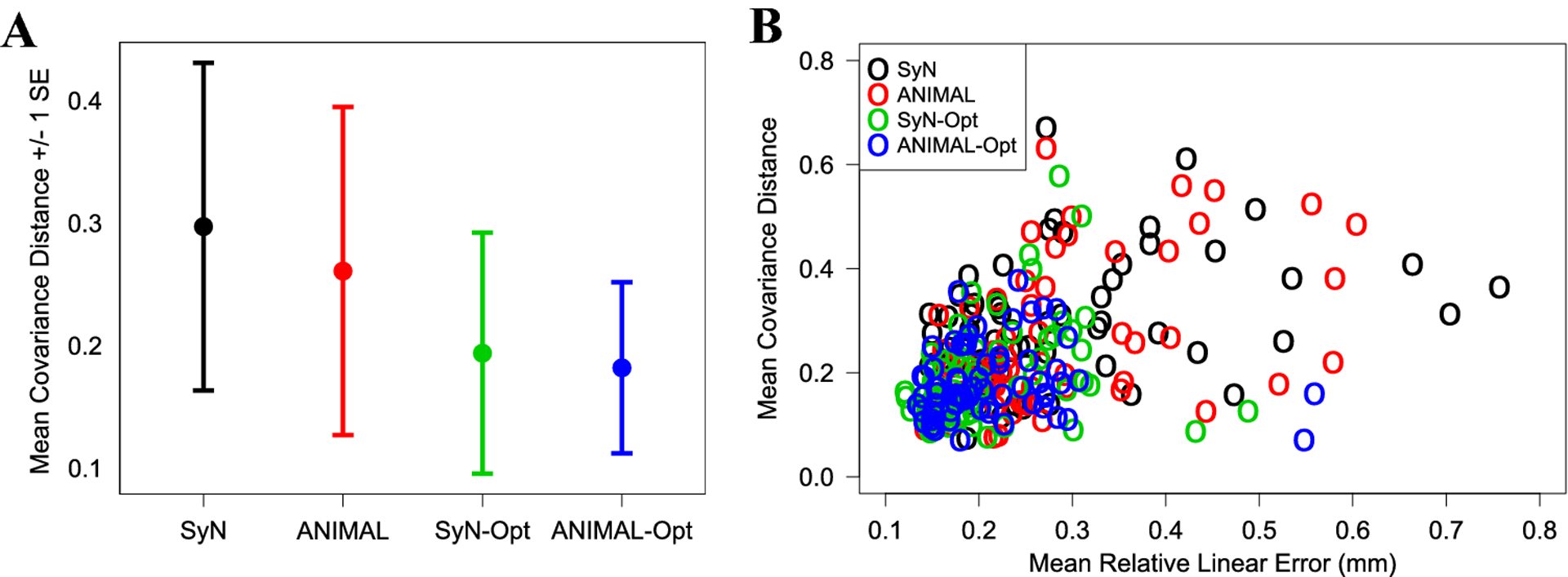
(A) The mean automated and manual covariance distance +/− one standard error (SE) across all landmarks. (B) The relationship between mean covariance distance and mean relative linear error at each landmark across automated workflows.
It is not unreasonable to assume that landmarks detected further from their true position will, on average, exhibit larger distribution errors. We found that this assumption holds true for the majority of problematic landmarks, which exhibited above average distribution errors (Fig. S4). However, the relationship between relative linear error and distribution error among all landmarks is fairly weak (r = 0.47) (Fig. 5B), indicating the two properties are not always related. In fact, the optimized distance-distribution correlation (r = 0.17) is much lower than the unoptimized correlation (r = 0.47). Locally accurate, yet imprecise landmark detection is a frequently overlooked phenomenon that could explain loss of biological signal during automation.
In our MANOVA of shape coordinates, method explained 26.1% of the total variance and was statistically significant (F = 19.84, p < 0.001), indicating that the mean shapes produced by the automated and manual workflows were not all equal. Fig. 6A–B uses heatmaps to visualize primary locations of contrasts between the manual mean, the optimized means, and the statistically distinguishable unoptimized means. Much of the difference can be traced to large landmark detection errors near the anterior and superior skull. Inspection of the specimen ordinations on the primary axes of shape variation for the MANOVA fitted values revealed that optimized and manually landmarked specimens closely overlap on PCs 1 and 2, whereas unoptimized configurations occupy a distinct region of the PC1 morphospace (Fig. 6C).
Fig. 6:
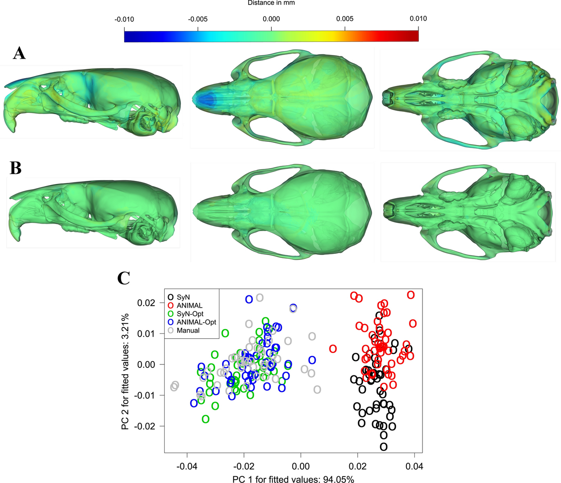
Heatmaps of (A) unoptimized and (B) optimized automated-manual contrasts at every vertex of the mean shape mesh. (C) A PCA on the shape vs. workflow fitted values obtained from the MANOVA.
To obtain further insight from the MANOVA, we examined mean shape distances and vector correlations post-hoc (Table 3). We observed that the effect of automated method on distance from the manual mean is far greater in the unoptimized methods than in the optimized methods. The SyN and ANIMAL mean shapes deviated significantly from the manual mean by 2.36 mm (Z = 15.32, p = 0.01) and 2.43 mm (Z = 16.43, p = 0.01), respectively. By contrast, the SyN-Opt and ANIMAL-Opt mean shapes showed statistically indistinguishable deviations of 0.49 mm (Z = 0.09, p = 0.41) and 0.42 mm (Z = −0.51, p = 0.65), respectively. Mean vector correlations across the workflows were consistent with the Euclidean distance relationships. The mean SyN and ANIMAL landmark angles differed significantly from the mean manual angles by 2.61° (Z = 15.32, p = 0.01) and 2.69° (Z = 16.43, p = 0.01), respectively. The SyN-Opt and ANIMAL-Opt landmark angles exhibited statistically indistinguishable differences of 0.54° (Z = 0.09, p = 0.41) and 0.47° (Z = −0.51, p = 0.65), respectively.
Table 3.
Pairwise statistics from the MANOVA residual randomization procedure, including Euclidean distance (mm) and angle differences (°) between each automated mean shape and the manual mean shape.
| Workflow | Distance | Z | P-value | Angle | Z | P-value |
|---|---|---|---|---|---|---|
| SyN | 2.36 | 15.18 | 0.01 | 2.61 | 15.18 | 0.01 |
| ANIMAL | 2.43 | 16.28 | 0.01 | 2.69 | 16.28 | 0.01 |
| SyN-Opt | 0.49 | 0.09 | 0.41 | 0.54 | 0.09 | 0.41 |
| ANIMAL-Opt | 0.42 | −0.51 | 0.65 | 0.47 | −0.51 | 0.65 |
P < 0.05 indicates the values are significantly different from the manual.
We evaluated automated-manual correlations of specimen ordinations on the first six PCs (collectively, 60.4% of manual variance; Fig. 7A), because they captured the majority of the sample variance. The average automated-manual correlations were very high across workflows on PCs 1 (r = 0.93) and 2 (r = 0.84) (Fig. 7B). They dropped on PC 3 (r = 0.50), but remained reasonably high on PCs 4 (r = 0.68), 5 (r = 0.63), and 6 (r = 0.61). Automated-manual PC correlations tended to be more similar across workflows on higher ranked PCs (PCs 1–4 correlation variance 0.001–0.003) than on lower ranked PCs (PCs 5–6 correlation variance 0.02). The conventional SyN and ANIMAL shape variances were 39.9% and 33.7% lower than the manual variance, respectively, whereas the SyN-Opt and ANIMAL-Opt variances were 37.2% and 28.9% lower, respectively (Fig. 8A). Automated variances were higher than the manual variance on relative PCs 1 and 2, particularly when unoptimized, before experiencing a steady decline from relative PC 3 onwards (Fig. 8B). The automated shape features most affected by this loss of variance were anteroposterior length and vault height (Fig. S5). This is not surprising, given that the most problematic landmarks (e.g., landmarks 2, 48, 49, 50, 51) reside around the anterior-most, posterior-inferior-most, and superior-most points of the skull.
Fig. 7:
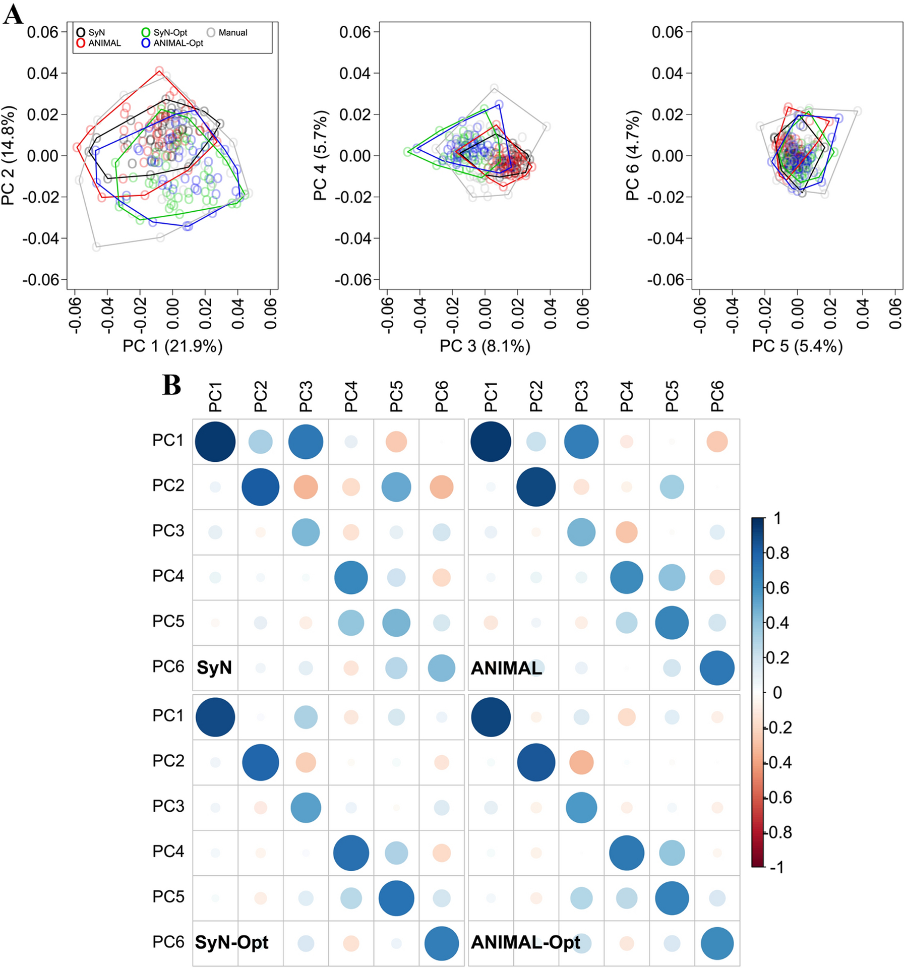
Automated configurations were rotated into the manual PC space after computing workflow-specific PCAs. (A) Convex hulls illustrating the distribution of variance along PCs 1 to 6. (B) Automated and manual PC score correlations for the first six PCs.
Fig. 8:
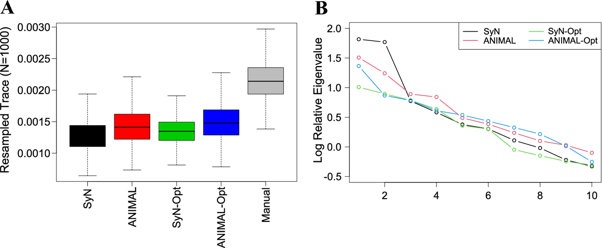
(A) Estimates of the sample variance for each method obtained by repeatedly resampling the trace of each covariance matrix. (B) Relative eigenvalues (on a log scale) of the automated landmark datasets relative to the manual. A value of 1 indicates equal variance, whereas values greater than or less than 1 correspond to increases and decreases in variance, respectively.
Discussion
Image registration, or the spatial alignment of images, is a well-established approach in biomedical imaging for automated phenotyping (Sotiras et al., 2013; Oliveira and Tavares, 2014). By establishing direct spatial correspondences, registration offers a common space for homologous data acquisition in anatomical context. In addition, atlases encourage data standardization, a prerequisite for large-scale GM analyses of morphological patterns, such as integration, modularity, and canalization (Hallgrimsson et al., 2009a, 2019a,b; Klingenberg 2008, 2009). Unfortunately, non-linear transformations are error-prone near morphologically variable locations (Heckemann et al. 2006). This leads to poor landmark detection and a loss of biological signal (Percival et al. 2019). It was therefore no surprise that our conventional registration-based landmark data showed notable deviations from the expert manual data in terms of individual and mean shape representations, sample-wide distance relationships, and variance-covariance patterns. To minimize automated landmark detection error, we introduced a framework that combines techniques from image registration, GM, and deep learning.
Applying our 0.25 mm automated-manual error criterion to the unoptimized data, 58/68 (85.3%) landmarks were classified as acceptable for SyN and 56/68 (82.3%) for ANIMAL. All 10 problematic SyN landmarks were problematic for ANIMAL, indicating that the choice of deformable registration makes little difference for placement of automated landmarks in error-prone regions. Among these shared landmarks, the highest detection errors were seen at the most anterior, superior, posterior-inferior points of the skull. Less error-prone, albeit still problematic, landmarks were found around the zygomatic arch. While 85.3% and 80.9% appear to be excellent acceptability rates, it is clear that the inclusion of problematic landmarks violates certain morphometric assumptions.
To improve landmark detection and morphometric outcomes, we trained a deep and domain-specific FFNN to learn a multi-output regression model that minimized automated-manual shape deviations. This optimization involved several GM processing steps. We performed separate GPAs of the training and testing data onto the manual mean shape, as it allowed the model learning and predictions to occur in the same shape space. In addition, we trained on Kendall’s tangent space coordinates, or Procrustes shape variables, because their linearity simplified the learning process, and their range ensured that each landmark contributed proportionately to the network loss function. The network loss function was driven by RMSE and balanced with a thin-plate spline bending energy term. RMSE was a sensible statistic to minimize, because it is globally differentiable and it measures the magnitude of error (i.e., the Procrustes distance) between a set of predicted shapes and the true mean shape. The mean shape plays a particularly important role in GM (Rohlf, 2003), because Procrustes superimposition minimizes each observation’s squared differences from it. Adding bending energy further ensured a smooth and differentiable transformation between corresponding landmark configurations.
Our deep learning approach was very successful at improving landmark detection. After accounting for manual error, both optimized registration workflows, SyN-Opt and ANIMAL-Opt, yielded landmark acceptability rates of 68/68 (100%). We significantly reduced automated-manual distance errors at all problematic locations and reduced average landmark deviations by 39.1% with both SyN-Opt and ANIMAL-Opt. Interestingly, our training subsamples (n=50 and n=100) yielded comparable reductions in average automated landmark deviation across the test set, suggesting that smaller samples could be used for training. However, we did not perform any GM tests on these data. Further work will need to focus on the composition (e.g., sample size and morphological diversity) and generalizability of landmark training sets, as deep FFNNs are prone to overfitting due to the presence of many network parameters.
Optimization also improved the distribution of individual observations around most automated landmarks. Using Procrustes shape covariance distance as a metric for distribution similarity, we observed that SyN-Opt and ANIMAL-Opt better reproduced the manual distribution of individual observations at 55/68 and 50/68 landmarks, respectively, compared to the conventional registration workflows. Optimized SyN performed the best, with a 36.7% reduction in average distribution error. The greatest distribution improvements were seen at problematic landmarks, where mean distance error magnitudes were largest. What was less expected, however, were low distance errors, yet relatively high distribution errors at several optimized landmarks. This suggests that detection can be accurate, but biased in particular directions, leading to local misrepresentations of morphology.
In addition to refining the detection and distribution of specific landmarks, our shape optimization increased the overall similarity of automated landmark configurations to their manual counterparts. This consequently led to significant improvements in the estimate of the mean shape, as well as distance relationships between each specimen and the mean shape. Specimen ordinations on the major PC axes were largely similar across workflows, but lower ranked PC ordinations were slightly improved via optimization. It was clear that automation reduced the sample shape variance, especially on lower order PCs. Reduced variance on lower order PCs could represent a minimization of measurement error and/or the inability of automated landmarks to capture subtle shape features. We did not test this hypothesis, because Percival and colleagues (2019) previously showed, using a similar registration framework, that 70% of the manual landmark variance corresponds to what is captured by automated landmarking and that the majority of the lost variance is attributable to the minimization of measurement error via automation.
Large and small deformable registration algorithms (e.g., SyN and ANIMAL) are fundamentally different in their approach to non-linear alignment. Whereas SyN seeks to maximize intensity similarity in across the entire displacement field using a shape manifold (diffeomorphism) that an image pair can symmetrically flow along, ANIMAL attempts to maximize similarity through local, piece-wise displacements. Because SyN was shown to be the top-performing deformable registration algorithm in a comparative study (Klein et al., 2009), we assumed it would outperform ANIMAL in all regards. However, the ANIMAL-Opt landmark data were statistically indistinguishable from the SyN-Opt data across most tests. These negligible differences are a welcome result, because they speak to the generality of our approach and that a majority of deformable registration algorithms can be used with confidence.
Any sample of homologous anatomical volumes, whether hard or soft tissue, can be subjected to an image registration pipeline to generate landmark configurations in an automated and unbiased manner. Other morphological information, such as segmentations and deformation fields, can be acquired alongside landmarks if desired. Complete spatial normalization also provides the flexibility to define landmark configurations of arbitrary dimensionality, allowing for sparse or dense shape analyses. This could open up novel opportunities for dense landmark GM, which is a poorly explored area due to the difficulty of establishing landmark homology. While the benefits of a registration and learning-based approach to landmark detection are clear, it must be underscored that poor anatomical homology (e.g., embryos at different stages), scanning artifacts, and inherent alignment functions (e.g., interpolation) can induce misalignment errors, resulting in landmark misdetection. In addition, poor replicability of manual landmark training sets may impair or bias the learning process, leading to inaccurate test set predictions. In the future, it will be important to validate the effectiveness of our approach in different imaging and morphometric contexts.
Conclusion
We introduced an approach that combines image registration, GM, and deep learning to automate and optimize landmark detection. Using standard morphometric tests, we demonstrated that our landmark optimization improves individual and mean representations of shape, sample-wide distance relationships, and variance-covariance patterns. While we tested and validated our method on high-resolution μCT images of the laboratory mouse skull, it should be recognized that this approach is generalizable to other volumetric imaging modalities, organisms, and anatomy. Given that our approach significantly improved landmark detection across the entire configuration, the reader should be confident in generalizing this method to any number of landmarks, so long as the manual landmark training set is reliable. Any GM researcher working in the context of phenomics, deep phenotyping, or other big data initiatives stands to benefit from the automaticity and accuracy of our approach. Our code is freely available at https://github.com/jaydevine/Landmarking.
Supplementary Material
Fig. S1: PCA of the 10 genetic atlas groups with convex hulls illustrating their distribution of variance along PCs 1 to 6.
Fig. S2: Procrustes distance to the grand mean shape. Distribution of the (A) entire database and (B) test image subset.
Fig. S3: Average landmark deviation, or RMSE, between each automated configuration and their corresponding manual configuration. We train the networks on homologous subsamples (n=50; n=100) to better understand the effects of training sample size on error.
Fig. S4: A summary of automated-manual covariance distances at problematic landmarks. We embed a mean covariance distance line to emphasize the above average increase in distributional error at problematic locations.
Fig. S5: Visualization of shape patterns (magnified 5x) along relative PCs using thin-plate spline deformation grids. The first relative PC shows the maximal excess of variance in automated landmarks relative manual landmarks, whereas the third and sixth relative PCs show the maximal excess of variance in manual landmarks relative to automated landmarks.
Funding
This work was supported by National Institutes of Health R01 01DE019638 to BH and RM, the Canadian Institutes of Health Research Foundation grant, the Natural Sciences and Engineering Research Council grant 238992–17, and the Canadian Foundation for Innovation grant #36262 to BH.
Footnotes
Publisher's Disclaimer: This Author Accepted Manuscript is a PDF file of an unedited peer-reviewed manuscript that has been accepted for publication but has not been copyedited or corrected. The official version of record that is published in the journal is kept up to date and so may therefore differ from this version.
Conflicts of interest
The authors have no conflicts of interest to declare.
Availability of data and material
Our training and testing images are available at https://www.facebase.org.
Code availability
Our code is freely available at https://github.com/jaydevine/Landmarking.
References
- Adams DC, Rohlf FJ, & Slice DE (2004). Geometric morphometrics: Ten years of progress following the ‘revolution’. Ital. J. Zool, 71(1), 5–16. 10.1080/11250000409356545 [DOI] [Google Scholar]
- Adams DC, Rohlf FJ, & Slice DE (2013). A Field Comes of Age: Geometric Morphometrics in the 21st Century. Hystrix, 24(1), 7–14. 10.4404/hystrix-24.1-6283 [DOI] [Google Scholar]
- Attanasio C, Nord AS, Zhu Y, Blow MJ, Li Z, Denise K, Morrison H, … Visel A (2014). Fine Tuning of Craniofacial Morphology by Distant-Acting Enhancers. Science, 342(6157), 1–20. 10.1126/science.1241006 [DOI] [PMC free article] [PubMed] [Google Scholar]
- Bates D, Machler M, Bolker B, & Walker S (2015). Fitting Linear Mixed-Effects Models Using lme4. J. Stat. Softw, 67(1), 1–48. 10.18637/jss.v067.i01 [DOI] [Google Scholar]
- Bezanson J, Edelman A, Karpinski S, & Shah VB (2017). Julia: A Fresh Approach to Numerical Computing. Siam. Rev, 59(1), 65–98. 10.1137/141000671 [DOI] [Google Scholar]
- Bookstein FL (1989). Principal Warps: Thin-Plate Splines and the Decomposition of Deformations. IEEE T. Pattern Anal, 11(6), 567–585. [Google Scholar]
- Bookstein FL (1991). Morphometric Tools for Landmark Data: Geometry and Biology. Cambridge: Cambridge University Press. [Google Scholar]
- Bookstein FL, & Mitteroecker P (2014). Comparing Covariance Matrices by Relative Eigenanalysis, with Applications to Organismal Biology. Evol. Biol, 41(2), 336–350. 10.1007/s11692-013-9260-5 [DOI] [Google Scholar]
- Bowman AW, & Azzalini A (1997). Applied Smoothing Techniques for Data Analysis: The Kernel Approach with S-Plus Illustrations. New York: Oxford University Press. [Google Scholar]
- Bromiley PA, Schunke AC, Ragheb H, Thacker NA, & Tautz D (2014). Semi-Automatic Landmark Point Annotation for Geometric Morphometrics. Front. Zool, 11(1), 61 10.1186/s12983-014-0061-1 [DOI] [Google Scholar]
- Bycroft C, Freeman C, Petkova D, Band G, Elliott LT, Sharp K, Motyer A, … Young A (2018). The UK Biobank Resource with Deep Phenotyping and Genomic Data. Nature, 562(7726), 203 10.1038/s41586-018-0579-z [DOI] [PMC free article] [PubMed] [Google Scholar]
- Collins DL, & Evans AC (1997). ANIMAL: Validation and Applications of Nonlinear Registration-Based Segmentation. Int. J. Pattern Recogn, 11(8), 1271–1294. [Google Scholar]
- Collyer ML, & Adams DC (2018). RRPP: An R Package for Fitting Linear Models High-Dimensional Data Using Residual Randomization. Methods Ecol. Evol, 9(7), 1772–1779. https://doi/10.1111/2041-210X.13029 [Google Scholar]
- Collyer ML, & Adams DC (2019). RRPP: Linear Model Evaluation with Randomized Residuals in a Permutation Procedure. R package version 0.4.0. [WWW Document]. URL https://cran.r-project.org/package=RRPP
- Duchon J (1976). Interpolation Des Fonctions De Deux Variables Suivant Le Principe De La Flexion Des Plaques Minces. Analyse Numerique, 10(R3), 5–12. [Google Scholar]
- Dryden IL (2018) shapes: Statistical Shape Analysis. R package version 1.2.4. [WWW Document]. URL https://CRAN.R-project.org/package=shapes
- Dryden IL, Koloydenko A, & Zhou D (2009). Non-Euclidean statistics for covariance matrices, with applications to diffusion tensor imaging. Ann. Appl. Stat, 3(3), 1102–1123. 10.1214/09-AOAS249 [DOI] [Google Scholar]
- Dryden IL, & Mardia KV (1998). Statistical Shape Analysis. London: Wiley. [Google Scholar]
- Evans AC, Janke AL, Collins DL, & Baillet S (2012). Brain Templates and Atlases. NeuroImage, 62(2), 911–922. 10.1016/j.neuroimage.2012.01.024 [DOI] [PubMed] [Google Scholar]
- Freimer N, & Sabatti C (2003). The Human Phenome Project. Nat. Genet, 34(1), 15–21. [DOI] [PubMed] [Google Scholar]
- Friedel M, van Eede MC, Pipitone J, Chakravarty MM, & Lerch JP (2014). Pydpiper: A Flexible Toolkit for Constructing Novel Registration Pipelines. Frontiers in Neuroinformatics, 8, 67 10.3389/fninf.2014.00067 [DOI] [PMC free article] [PubMed] [Google Scholar]
- Gower JC (1975). Generalized Procrustes Analysis. Psychometrika, 40(1), 33–50. [Google Scholar]
- Hallgrímsson B, Willmore K, Dorval C, & Cooper DML (2004). Craniofacial Variability and Modularity in Macaques and Mice. J. Exp. Zool. Part B, 302(3), 207–225. 10.1002/jez.b.21002 [DOI] [PubMed] [Google Scholar]
- Hallgrímsson B, Brown JJ, Ford-Hutchinson AF, Sheets HD, Zelditch ML, & Jirik FR (2006). The Brachymorph Mouse and the Developmental-Genetic Basis for Canalization and Morphological Integration. Evol. Dev, 8(1), 61–73. 10.1111/j.1525-142X.2006.05075.x [DOI] [PubMed] [Google Scholar]
- Hallgrímsson B, Jamniczky H, Young NM, Rolian C, Parsons TE, Boughner JC, & Marcucio RS (2009). Deciphering the Palimpsest: Studying the Relationship Between Morphological Integration and Phenotypic Covariation. Evol. Biol, 36(4), 355–376. 10.1007/s11692-009-9076-5 [DOI] [PMC free article] [PubMed] [Google Scholar]
- Hallgrímsson B, Boughner JC, Turinsky AL, & Sensen CW (2009). Geometric Morphometrics and the Study of Development, in: Sensen CW, Hallgrímsson B (Eds.), Advanced Imaging in Biology and Medicine. Berlin, Springer-Verlag, pp. 319–336. 10.1007/978-3-540-68993-5 [DOI] [Google Scholar]
- Hallgrímsson B, Green RM, Katz DC, Fish JL, Bernier FP, Roseman CC, Young NM, Cheverud JM, & Marcucio RS (2019). The Developmental-Genetics of Canalization. Semin. Cell. Dev. Biol, 88, 67–79. https://doi.org/10.1016Zj.semcdb.2018.05.019 [DOI] [PMC free article] [PubMed] [Google Scholar]
- Hallgrímsson B, Katz DC, Aponte JD, Larson JR, Devine J, Gonzalez PN, Young NM, Roseman CC, & Marcucio RS (2019). Integration and the Developmental Genetics of Allometry. Integr. Comp. Biol, 59(5), 1369–1381. 10.1093/icb/icz105 [DOI] [PMC free article] [PubMed] [Google Scholar]
- Heckemann RA, Hajnal JV, Aljabar P, Rueckert D, & Hammers A (2006). Automatic Anatomical Brain MRI Segmentation Combining Label Propagation and Decision Fusion. NeuroImage, 33(1), 115–126. 10.1016/j.neuroimage.2006.05.061 [DOI] [PubMed] [Google Scholar]
- Houle D, Govindaraju DR, & Omholt S (2010). Phenomics: The Next Challenge. Nat. Rev. Genet, 11(12), 855–866. 10.1038/nrg2897 [DOI] [PubMed] [Google Scholar]
- Innes M (2018). Flux: Elegant Machine Learning with Julia. J. Open Source Softw, 3(25), 602 10.21105/joss.00602 [DOI] [Google Scholar]
- Kendall DG (1984). Shape Manifolds, Procrustean Metrics and Complex Projective Spaces. Bull. Lond. Math Soc, 16(2), 81–121. [Google Scholar]
- Kingma DP, & Ba JL (2015). Adam: A Method for Stochastic Optimization. arXiv preprint arXiv: 1412.6980.
- Klein A, Andersson J, Ardekani BA, Ashburner J, Avants B, Chiang MC, … & Song JH (2009). Evaluation of 14 Nonlinear Deformation Algorithms Applied to Human Brain MRI Registration. NeuroImage, 46(3), 786–802. 10.1016/j.neuroimage.2008.12.037 [DOI] [PMC free article] [PubMed] [Google Scholar]
- Klingenberg CP (2002). Morphometrics and the Role of the Phenotype in Studies of the Evolution of Developmental Mechanisms. Gene, 287(1–2), 3–10. 10.1016/S0378-1119(01)00867-8 [DOI] [PubMed] [Google Scholar]
- Klingenberg CP (2008). Morphological Integration and Developmental Modularity. Annu. Rev. Eeol. Evol. S, 39, 115–132. 10.1146/annurev.eeolsys.37.091305.110054 [DOI] [Google Scholar]
- Klingenberg CP (2009). Morphometric Integration and Modularity in Configurations of Landmarks: Tools for Evaluating A Priori Hypotheses. Evol. Dev, 11(4), 405–421. 10.1111/j.1525-142X.2009.00347 [DOI] [PMC free article] [PubMed] [Google Scholar]
- Le Maître A & Mitteroecker P (2019). Multivariate Comparison of Variance in R. Methods Ecol. Evol, 10(9), 1380–1392. 10.1111/2041-210X.13253 [DOI] [Google Scholar]
- Li M, Cole JB, Manyama M, Larson JR, Liberton DK, Riccardi SL, Ferrara TM, … Hallgrímsson B (2017). Rapid Automated Landmarking for Morphometric Analysis of Three-Dimensional Facial Scans. J. Anat, 230(4), 607–618. 10.1111/joa.12576 [DOI] [PMC free article] [PubMed] [Google Scholar]
- Lieberman DE, Hallgrímsson B, Liu W, Parsons TE, & Jamniczky HA (2008). Spatial Packing, Cranial Base Angulation, and Craniofacial Shape Variation in the Mammalian Skull: Testing a New Model Using Mice. J. Anat, 212(6), 720–735. 10.1111/j.1469-7580.2008.00900.x [DOI] [PMC free article] [PubMed] [Google Scholar]
- Maga AM, Tustison NJ, & Avants BB (2017). A Population Level Atlas of Mus Musculus Craniofacial Skeleton and Automated Image-Based Shape Analysis. J. Anat, 231(3), 433–443. 10.1111/joa.12645 [DOI] [PMC free article] [PubMed] [Google Scholar]
- Mazziotta J, Toga A, Evans A, Fox P, Lancaster J, Zilles K, Woods, … Mazoyer B. (2001). A Probabilistic Atlas and Reference System for the Human Brain: International Consortium for Brain Mapping (ICBM). Philos. T. Roy. Soc. B, 356, 1293–1322. 10.1098/rstb.2001.0915 [DOI] [PMC free article] [PubMed] [Google Scholar]
- Mitteroecker P, & Gunz P (2009). Advances in Geometric Morphometrics. Evol. Biol, 36(2), 235–247. 10.1007/s11692-009-9055-x [DOI] [Google Scholar]
- Nelder JA, & Mead R (1965). A Simplex Method for Function Minimization. The Computer Journal. 7(4), 308–313. [Google Scholar]
- Oksanen J, Blanchet FG, Friendly M, Kindt R, Legendre P, McGlinn D, Minchin PR, … Wagner H (2019). vegan: Community Ecology Package. R package version 2.5–4. [WWW Document]. URL https://cran.r-project.org/package=vegan
- Oliveira FP, & Tavares JMR (2014). Medical Image Registration: A Review. Comput. Method Biomec, 17(2), 73–93. 10.1080/10255842.2012.670855 [DOI] [PubMed] [Google Scholar]
- O’Higgins P, Chadfield P, & Jones N (2001). Facial Growth and the Ontogeny of Morphological Variation Within and Between the Primates Cebus Apella and Cercocebus Torquatus. J. Zool, 254(3), 337–357. [Google Scholar]
- Percival CJ, Green R, Marcucio R, & Hallgrímsson B (2014). Surface Landmark Quantification of Embryonic Mouse Craniofacial Morphogenesis. BMC Dev. Biol, 14(1), 31 10.1186/1471-213X-14-31 [DOI] [PMC free article] [PubMed] [Google Scholar]
- Percival CJ, Devine J, Darwin BC, Liu W, van Eede M, Henkelman RM, & Hallgrímsson B (2019). The Effect of Automated Landmark Identification on Morphometric Analyses. J. Anat, 234(6), 917–935. 10.1111/joa.12973 [DOI] [PMC free article] [PubMed] [Google Scholar]
- Raup DM (1966). Geometric Analysis of Shell Coiling. J. Paleont, 40(5), 1178–1190. [Google Scholar]
- R Core Team (2018). R: A Language and Environment for Statistical Computing. Vienna: R Foundation for Statistical Computing. [WWW Document]. URL https://www.R-project.org/.
- Robinson PN (2012). Deep Phenotyping for Precision Medicine. Hum. Mutat., 3395), 777–780. 10.1002/humu.22080 [DOI] [PubMed]
- Rohlf FJ (2003). Bias and Error in Estimates of Mean Shape in Geometric Morphometrics. J. Hum. Evol, 44(6), 665–683. 10.1016/S0047-2484(03)00047-2 [DOI] [PubMed] [Google Scholar]
- Rohlf FJ, & Slice D (1990). Extensions of the Procrustes Method for the Optimal Superimposition of Landmarks. Syst. Biol, 39(1), 40–59. [Google Scholar]
- Rohlfing T, & Maurer CR (2006). Shape-Based Averaging. IEEE T. Image Process, 16(1), 153–161. [DOI] [PubMed] [Google Scholar]
- Rueckert D, Sonoda LI, Hayes C, Hill DLG, Leach MO, & Hawkes DJ (1999). Nonrigid Registration Using Free-Form Deformations: Application to Breast MR Images. IEEE T. Med. Imaging, 18(8), 712–721. [DOI] [PubMed] [Google Scholar]
- Schlager S (2017). Morpho and Rvcg – Shape Analysis in R: R-Packages for Geometric Morphometrics, Shape Analysis and Surface Manipulations, in: Zheng G, Li S, Szekely G (Eds.), Statistical Shape and Deformation Analysis. Cambridge, Academic Press, pp. 217–256. 10.1016/B978-0-12-810493-4.00011-0 [DOI] [Google Scholar]
- Schork NJ (1997). Genetics of Complex Disease: Approaches, Problems, and Solutions. Am. J. Resp. Crit. Care, 156(4), S103–S109. [DOI] [PubMed] [Google Scholar]
- Sotiras A, Davatzikos C, & Paragios N (2013). Deformable Medical Image Registration: A Survey. IEEE T. Med. Imaging, 32(7), 1153–1190. [DOI] [PMC free article] [PubMed] [Google Scholar]
- Vincent RD, Neelin P, Khalili-Mahani N, Janke AL, Fonov VS, Robbins SM, Baghdadi L, … Abbott DF (2016). MINC 2.0: A Flexible Format for Multi-Modal Images. Front. Neuroinform, 10, 35 10.3389/fninf.2016.00035 [DOI] [PMC free article] [PubMed] [Google Scholar]
- von Cramon-Taubadel N, Frazier BC, & Lahr MM (2007). The Problem of Assessing Landmark Error in Geometric Morphometrics: Theory, Methods, and Modifications. Am. J. Phys. Anthropol, 134(1), 24–35. 10.1002/ajpa.20616 [DOI] [PubMed] [Google Scholar]
- Vora SR, Camci ED, & Cox TC (2016). Postnatal Ontogeny of the Cranial Base and Craniofacial Skeleton in Male C57BL/6J Mice: A Reference Standard for Quantitative Analysis. Front. Physiol, 6, 417 10.3389/fphys.2015.00417 [DOI] [PMC free article] [PubMed] [Google Scholar]
- Wang H, Suh JW, Das SR, Pluta JB, & Yushkevich PA (2012). Multi-Atlas Segmentation with Joint Label Fusion. IEEE T. Pattern Anal, 35(3), 611–623. 10.1109/TPAMI.2012.143 [DOI] [PMC free article] [PubMed] [Google Scholar]
- Wei T, & Simko V (2017). R package “corrplot”: Visualization of a correlation matrix. R package version 0.84. [WWW Document]. URL https://github.com/taiyun/corrplot. [Google Scholar]
- Young R, & Maga AM (2015). Performance of Single and Multi-Atlas Based Automated Landmarking Methods Compared to Expert Annotations in Volumetric microCT Datasets of Mouse Mandibles. Front. Zool, 12(1), 33 10.1186/s12983-015-0127-8 [DOI] [PMC free article] [PubMed] [Google Scholar]
- Zelditch ML, Swiderski DL, Sheets HD, & Fink WL (2012). Geometric Morphometrics for Biologists: A Primer. San Diego: Elsevier Academic Press. [Google Scholar]
Associated Data
This section collects any data citations, data availability statements, or supplementary materials included in this article.
Supplementary Materials
Fig. S1: PCA of the 10 genetic atlas groups with convex hulls illustrating their distribution of variance along PCs 1 to 6.
Fig. S2: Procrustes distance to the grand mean shape. Distribution of the (A) entire database and (B) test image subset.
Fig. S3: Average landmark deviation, or RMSE, between each automated configuration and their corresponding manual configuration. We train the networks on homologous subsamples (n=50; n=100) to better understand the effects of training sample size on error.
Fig. S4: A summary of automated-manual covariance distances at problematic landmarks. We embed a mean covariance distance line to emphasize the above average increase in distributional error at problematic locations.
Fig. S5: Visualization of shape patterns (magnified 5x) along relative PCs using thin-plate spline deformation grids. The first relative PC shows the maximal excess of variance in automated landmarks relative manual landmarks, whereas the third and sixth relative PCs show the maximal excess of variance in manual landmarks relative to automated landmarks.