Abstract
Dry weight is the normal weight of hemodialysis patients after hemodialysis. If the amount of water in diabetes is too much (during hemodialysis), the patient will experience hypotension and shock symptoms. Therefore, the correct assessment of the patient's dry weight is clinically important. These methods all rely on professional instruments and technicians, which are time-consuming and labor-intensive. To avoid this limitation, we hope to use machine learning methods on patients. This study collected demographic and anthropometric data of 476 hemodialysis patients, including age, gender, blood pressure (BP), body mass index (BMI), years of dialysis (YD), and heart rate (HR). We propose a Sparse Laplacian regularized Random Vector Functional Link (SLapRVFL) neural network model on the basis of predecessors. When we evaluate the prediction performance of the model, we fully compare SLapRVFL with the Body Composition Monitor (BCM) instrument and other models. The Root Mean Square Error (RMSE) of SLapRVFL is 1.3136, which is better than other methods. The SLapRVFL neural network model could be a viable alternative of dry weight assessment.
1. Introduction
Fluid overload in patients with chronic renal failure is closely related to poor cardiovascular outcomes [1, 2]. Maintenance of hemodialysis (HD) is the main method for patients with renal failure [3]. However, the accurate assessment of body water volume is still a concern [4]. At present, dry weight has been used as an important indicator to assess the homeostasis of fluids in hemodialysis patients. Medical staff can use the patient's dry weight to estimate the amount of water needed for dialysis during hemodialysis. The conventional clinical-based dry weight assessment method is time-consuming and labor-intensive [1]. There are already some methods based on bioelectrical impedance analysis (BIA) [5] to determine dry weight, including body composition monitor (BCM) [6] and lung ultrasound (LUS). However, all the above methods require special instruments and professional technicians to complete. Medical staff can use some clinical data to build predictive models [7] to accurately assess dry weight. Currently, machine learning (ML) or deep learning has solved many common clinical problems in medicine, such as brain diseases [8–10], cancer analysis, and diabetes.
Some scholars have used artificial neural networks (ANN) to predict the total water volume of hemodialysis patients and have obtained better results than conventional clinical calculation equations [11]. In addition, deep learning methods are also emerging in clinical diagnosis, including pixel-based convolutional neural networks to diagnose skin cancer [12]. In the biological field, microbiology analysis [13], CircRNAs [14], microRNAs, and cancer association prediction [15–17], lncRNA-miRNA association prediction, O-GlcNAcylation site prediction [18], DNA methylation site [19–21], protein remote homology [22], function prediction of proteins [23–29], electron transport proteins [30], breast cancer [31], cell-specific replication [32], osteoporosis diagnoses [33], and drug complex network analysis [34–38].
In our previous research, a Multiple Kernel Support Vector Regression (MKSVR) [39] predictor was proposed to assess the dry weight and obtain good predictive performance. Inspired by the previous work and baseline Random Vector Functional Link (RVFL) network [40], we propose a new dry weight assessment model, called Sparse Laplacian regularized RVFL neural network with L2,1-norm (SLapRVFL), which considers the topological relationship between samples and more sparse connections between the input layer and the hidden layer.
2. Materials and Methods
2.1. Materials
This work collects demographic and anthropometric data and bioimpedance spectroscopy (BIS) from historical data (2018-9 to 2019-9) from Wuxi people's hospital and the northern Jiangsu people's hospital. This study has been approved by the ethics committees of the hospitals (Nos. KYLLKS201813 and 2018KY-001). The collected patient data meet the following requirements: age greater than 18 years; ESRD for more than three months and maintenance hemodialysis [41]; no heart failure, no metal implants, no pregnancy, no disability, no infection, and no edema and other diseases; and hemodialysis treatment 3 times a week, 4 hours each time. Finally, we obtain a data set of 476 hemodialysis patients. DW is the normal body weight after clinical diabetes. DW is obtained by a clinician under strict clinical supervision using a clinical scoring system (using trial and error method) [42, 43].
We choose 7 features, including age, gender (binary feature), systolic blood pressure (SBP), diastolic blood pressure (DBP), body mass index (BMI), heart rate (HR), and years of dialysis (YD) to build our predictive model. Table 1 shows the information of the data set. BMI is measured before hemodialysis treatment.
Table 1.
The information of data set.
| Feature | Value | r ∗ |
|---|---|---|
| Age (years) | 54.17 ± 14.22 | -0.2341 |
| Gender (males/females) | 312/164 | -0.4489 |
| BMI | 22.96 ± 2.95 | 0.9558 |
| Systolic blood pressure (mmHg) | 150.64 ± 29.36 | -0.1739 |
| Diastolic blood pressure (mmHg) | 88.32 ± 19.56 | -0.1249 |
| Heart rate (times/min) | 73.41 ± 8.92 | 0.1862 |
| Years of dialysis (years) | 5.97 ± 3.22 | -0.1069 |
∗Denotes that each feature correlated with dry weight using Pearson correlation coefficient (r).
2.2. Methods
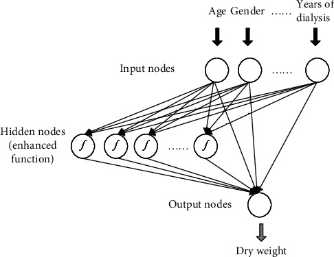
The baseline RVFL was proposed for regression or classification. The schematic diagram of RVFL is shown in Figure 1. The basic information of the patient is put into the RVFL neural network model for processing, and the predicted dry weight is the output.
Figure 1.
Schematic of our proposed method.
Suppose, there are N training samples with {xi, yi}, i = 1, 2, ⋯, N. The output value is yi ∈ R1×c and the input data is xi ∈ R1×d. d denotes the dimension of xi. As per Figure 1, RVFL randomly initializes all weights and deviations between the hidden layer and the input layer. These parameters are fixed during the training process and do not need to be tuned. There are connections between the output layer, input layer, and hidden layer. This part of the weight needs to be obtained by training RVFL. The output layer of RVFL is connected to both the input layer and the hidden layer, so as to ensure the nonlinear and linear relationships between the input and the output. The RVFL network with P hidden nodes are formulated as
| (1) |
where β denotes the output weight matrix; H is the concatenated matrix, which combines the output of the hidden layer and the input layer; and Y denotes the label matrix. H and β can be represented as
| (2) |
| (3) |
| (4) |
| (5) |
In Equation (4), aj and bj are the weights and bias of the hidden and input layers. C and P are numbers of output and hidden layer nodes. In general, the activation function is a Gaussian function: g(x) = e−x2. The activation function has a nonlinear approximation effect. To consider the potential linear relationship between the input data and the output value, RVFL adds a direct connection weight between the input layer and the output layer. Therefore, RVFL is a model that contains both linear and nonlinear approximations to improve prediction performance. For optimal β, the RVFL can be formulated as a regularized least-squares:
| (6) |
where λ is the parameter of regularization term. The solution of Equation (6) can be found by setting its gradient to 0:
| (7) |
where I denotes the identity matrix. However, the RVFL network did not consider the topological relationship between samples. For the output node, it must be connected to both the input and the hidden layer.
In order to further improve the robustness of RVFL, we propose Sparse Laplacian regularized RVFL neural network with L2,1-norm (SLapRVFL). The objective function is
| (8) |
where L ∈ RN×N denotes the Laplacian matrix. λ1 and λ2 are the coefficients of Laplacian regularization the and L21-norm term, respectively. Laplacian regularization is used to indicate the potential manifold between samples. It can better describe the topological association between samples to improve the generalization ability of the model. Since the third term of ‖β‖2,12 is not diversified, we convert Equation (8) to
| (9) |
where G ∈ R(d + P)×(d + P) denotes a diagonal matrix whose ith-diagonal element
| (10) |
We take the derivative of the formula Equation (10) as
| (11a) |
| (11b) |
| (11c) |
| (11d) |
We use the baseline RVFL solution with Equation (7) as the initial β0. In addition, the Laplacian matrix can be calculate as
| (12a) |
| (12b) |
where D is diagonal matrix, Dii = ∑j=1NSij. Similarity matrix S is built by Radial Basis Function (RBF):
| (13) |
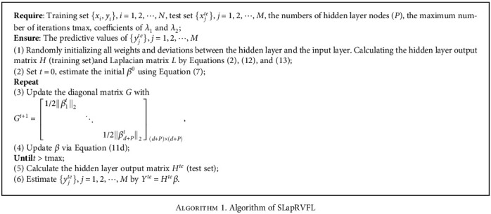
The process of SLapRVFL is list in Algorithm 1.
Algorithm 1.
Algorithm 1. Algorithm of SLapRVFL
3. Results
We test our model on the benchmark data set and obtain the optimal parameters of the predictor through cross-validation. The SLapRVFL network is compared to other machine learning-based models. In addition, the body composition monitor (BCM) device (Fresenius Medical Care, Baden Humboldt, Germany) is also compared with the SLapRVFL network.
3.1. Evaluation Measurements
The 10-fold cross-validation (10-CV) is employed to evaluate the robustness of methods. Root Mean Square Error (RMSE), R square, correlation coefficient (R), Bland–Altman analysis, and Empirical Cumulative Distribution Plot (ECDP) [44] are all used in our study. To evaluate the agreement of two different methods, the Bland–Altman analysis usually can obtain whether the two methods can be substituted for each other (equivalence). Evaluating the agreement of the two methods can answer the question, “Can these two methods replace each other?”
3.2. Selection of Optimal Parameters
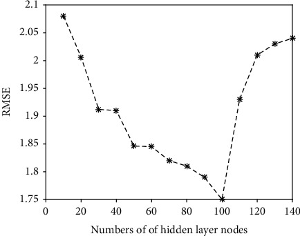
To get the optimal parameters of the predictive method, we obtain them through a grid search method. The parameters that need to be determined include the numbers of hidden layer nodes P, maximum iterations, and coefficients of λ1 and λ2. For the numbers of hidden layer nodes P, we fix the iterations, λ1 and λ2. Setting the maximum number as 50, λ1 = 1 and λ2 = 1. The value of P is from 10 to 140 with step of 10. The results are shown in Figure 2. From 10 to 100, the more neurons in the hidden layer, the lower the RMSE. Since then, RMSE has gradually increased. So, we get the lower RMSE under P = 100.
Figure 2.
The RMSE under different numbers of hidden layer nodes (SLapRVFL network).
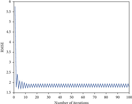
Next, P = 100, λ1 = 1, and λ2 = 1. We gradually increase the number of iterations from 1 to 100 (shown in Figure 3). After the number of iterations reaches 10, the RMSE value drops to a minimum and slightly oscillates within a certain value. In our study, maximum number of iterations is 10.
Figure 3.
The RMSE of iterations on the training set.
Then, we use the better number of hidden layer nodes and iterations to search for the best λ1 and λ2. The search range of parameters is from 2−5 to 20 (with step of 20.5). Figure 4 shows the results of different parameters. When λ1 and λ2 are 2−3 and 2−2.5, RMSE is the lowest.
Figure 4.
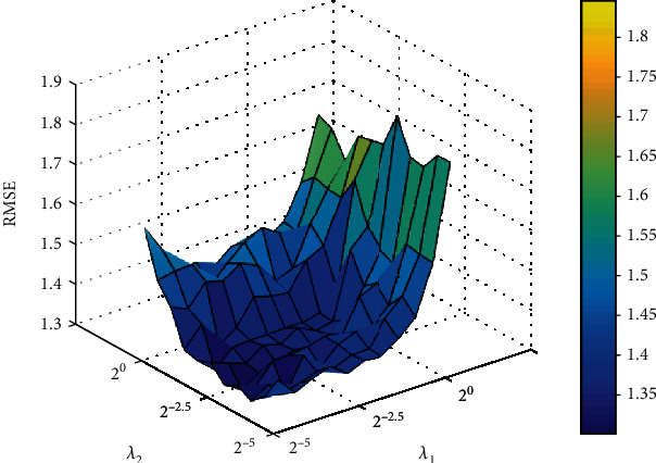
The RMSE under different λ1 and λ2.
3.3. Comparison to Other Predictive Models and BCM
To evaluate our model, SLapRVFL is compared with our previous work of Multiple Kernel Support Vector Regression (MKSVR) [39], Multikernel Ridge Regression (MKRR), Linear Regression (LR), Artificial Neural Network based on Back Propagation algorithm (ANN with BP), and BCM measuring instrument. Clinical dry weight is our reference standard (also the regression target value of the prediction model). The comparisons are listed in Table 2, which shows that SLapRVFL achieves best performance of RMSE (1.3136). Although the ECDP median value (peak) of MKSVR (0.0082) is more close to zero, Figure 5 shows that SLapRVFL has the least bias and much less tails than MKSVR (smaller width). The RMSE of BCM is 1.9694, which is larger than SLapRVFL.
Table 2.
Comparison on existing methods via 10-fold cross-validation.
| Method | R | R squared | RMSE | Empirical cumulative distribution plot | ||
|---|---|---|---|---|---|---|
| Highest value | Lowest value | Median value | ||||
| BCM∗ | 0.9473 | 0.9137 | 1.9694 | 3.2235 | -6.2776 | -0.9863 |
| LR∗ | 0.9403 | 0.9308 | 1.4335 | 4.2524 | -4.4014 | 0.1418 |
| ANN (BP)∗ | 0.9398 | 0.9295 | 1.4794 | 7.3661 | -4.7447 | 0.1324 |
| MKRR∗ | 0.9399 | 0.9289 | 1.5015 | 4.9227 | -4.2604 | 0.1104 |
| MKSVR∗ | 0.9412 | 0.9321 | 1.3817 | 4.3962 | -4.1273 | 0.0082 |
| RVFL | 0.9389 | 0.9300 | 1.3828 | 6.7004 | -4.3557 | 0.0704 |
| SLapRVFL (our method) | 0.9632 | 0.9501 | 1.3136 | 3.1940 | -3.5066 | 0.1014 |
∗The results are from previous work on MKSVR [39].
Figure 5.
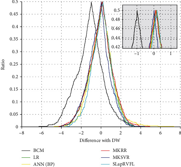
Folded empirical cumulative distribution plot between different methods.
3.4. Bland–Altman Analysis
Bland–Altman plot is a useful tool to evaluate the agreement between predictive methods and clinical DW. In Table 3 and Figure 6, SLapRVFL, MKSVR, LR, ANN (BP), MKRR, and BCM are analyzed via Bland-Altman difference plot. SLapRVFL achieves the smallest range of 95% confidence interval (-0.1133 to 0.2866) and standard deviation (2.2202). In addition, the number (ratio) of outside agreement interval for predictive models is all less than 24 (5%) predictive samples. These results of models are clinically acceptable. SLapRVFL achieves least number (20) of the outside agreement interval in Table 3. As shown in Figure 6, two red horizontal dotted lines (upper and lower) denote the upper and lower limits of the 95% agreement limit, respectively. The middle blue solid line is the average value of the difference (between measurement methods and clinical DW). While one measurement method and clinical method can be considered as a better agreement, they can be substituted for each other (equivalence). If 95% of the points of the data set are in the agreement range, the measurement method (predictive model) is clinically acceptable. The results of the evaluation show that SLapRVFL can help clinicians assess DW with low cost.
Table 3.
Bland–Altman plot analysis for different models.
| Model | Differences with DW (%) | Limits of agreement (%) | ||||
|---|---|---|---|---|---|---|
| Mean | SD | 95% confidence interval | Lower limit | Upper limit | Number (ratio) of outside agreement interval | |
| BCM∗ | -1.8232 | 2.7466 | -2.0706 to -1.5759 | -7.2066 | 3.5601 | 30/476 (6.30%) |
| LR∗ | 0.0002 | 2.4269 | -0.2184 to 0.2187 | -4.7566 | 4.7569 | 21/476 (4.41%) |
| ANN (BP)∗ | 0.1152 | 2.5139 | -0.1112 to 0.3416 | -4.8119 | 5.0424 | 22/476 (4.62%) |
| MKRR∗ | -0.0801 | 2.5007 | -0.3053 to 0.1451 | -4.9814 | 4.8212 | 23/476 (4.83%) |
| MKSVR∗ | -0.2638 | 2.3372 | -0.4743 to -0.05329 | -4.8446 | 4.3171 | 22/476 (4.62%) |
| SLapRVFL (our method) | 0.0867 | 2.2202 | -0.1133 to 0.2866 | -4.2650 | 4.4383 | 20/476 (4.20%) |
∗The results are from previous work on MKSVR [39].
Figure 6.
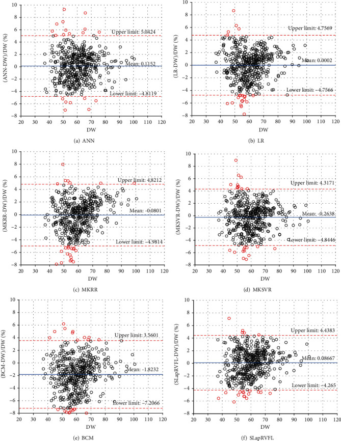
Bland–Altman plot analysis.
4. Discussion
Due to the limitations of clinical and BCM measurement (more time and cost), this study uses a machine learning method to assess the dry weight of hemodialysis patients. Based on the basic RVFL, we propose a sparse Laplace regularized RVFL network (SLapRVFL) model. SLapRVFL is compared not only with other machine learning methods (such as LR, MKRR, ANN with BP, and MKSVR) but also with BCM equipment (commonly used in hospitals). The RMSE and Bland–Altman analysis of the model are better than the BCM instrument. It is proven that the predictive model driven by data can provide reference for clinical dry weight assessment.
BCM requires the patient's information on weight (before hemodialysis) and height. It is a portable, inexpensive, and noninvasive technology that has been used to measure DW [45, 46]. For the Bland–Altman analysis, SLapRVFL achieves the least number (20) of outside agreement interval. However, BCM has 30/476 (6.30%) points (ratio) of the outside agreement interval. Obviously, our method has better agreement with the clinical method.
5. Conclusions
To further improve the robustness of RVFL, we introduce sparse Laplacian regular term with L2,1-norm. In the training process, the graph topology information and the sparse weight matrix (output) are employed to improve the robustness of the RVFL. In fact, our work provides a new idea for assessing patients' dry weight. Not only that, in the fields of biology [47–57], pharmacy [58], and medicine [12, 59, 60], machine learning methods have helped solve many analysis tasks. In future research, we will consider collecting more samples, introducing more patient personal information, and building a predictor based on a deep learning model to more accurately assess the dry weight of hemodialysis patients.
Acknowledgments
The authors give their thanks to the Hemodialysis Center of Wuxi People's Hospital and Northern Jiangsu People's Hospital for collecting the data in this study. This work is supported by a grant from the National Natural Science Foundation of China (NSFC 61902271, 61772362, and 61972280) and the Natural Science Research of Jiangsu Higher Education Institutions of China (19KJB520014).
Contributor Information
Wei Zhou, Email: 285403434@qq.com.
Yinghua Cai, Email: 179098331@qq.com.
Yijie Ding, Email: wuxi_dyj@163.com.
Data Availability
The data used to support the findings of this study are available from the corresponding author upon request.
Ethical Approval
This study had been approved by the ethics committee of the hospital (ethical approval Nos. KYLLKS201813 and 2018KY-001). The experimental protocol was established, according to the ethical guidelines of the Helsinki Declaration, and was approved by the Human Ethics Committee (Wuxi People's Hospital Ethics Committee and Northern Jiangsu People's Hospital Ethics Committee).
Consent
Written informed consent for publication was obtained from all participants.
Conflicts of Interest
The authors declare that they have no conflict of interest.
Authors' Contributions
Xiaoyi Guo and Wei Zhou are joint first authors.
References
- 1.Grassmann A., Uhlenbusch-Körwer I., Bonnie-Schorn E., Vienken J. Composition and management of hemodialysis fluids. Good Dialysis Practice. 2000;2:13–25. [Google Scholar]
- 2.Wabel P., Chamney P., Moissl U., Jirka T. Importance of whole-body bioimpedance spectroscopy for the management of fluid balance. Blood Purification. 2009;27(1):75–80. doi: 10.1159/000167013. [DOI] [PMC free article] [PubMed] [Google Scholar]
- 3.Alexiadis G., Panagoutsos S., Roumeliotis S., et al. Comparison of multiple fluid status assessment methods in patients on chronic hemodialysis. International Urology and Nephrology. 2016;49(3):1–8. doi: 10.1007/s11255-016-1473-y. [DOI] [PubMed] [Google Scholar]
- 4.Ohashi Y., Sakai K., Hase H., Joki N. Dry weight targeting: the art and science of conventional hemodialysis. Seminars in Dialysis. 2018;31 doi: 10.1111/sdi.12721. [DOI] [PubMed] [Google Scholar]
- 5.Asmat H., Iqbal R., Sharif F., Mahmood A., Abbas A., Kashif W. Validation of bioelectrical impedance analysis for assessing dry weight of dialysis patients in Pakistan. Saudi Journal of Kidney Diseases & Transplantation. 2017;28(2):p. 285. doi: 10.4103/1319-2442.202766. [DOI] [PubMed] [Google Scholar]
- 6.Jiang C., Patel S., Moses A., DeVita M. V., Michelis M. F. Use of lung ultrasonography to determine the accuracy of clinically estimated dry weight in chronic hemodialysis patients. International Urology and Nephrology. 2017;49(12):2223–2230. doi: 10.1007/s11255-017-1709-5. [DOI] [PubMed] [Google Scholar]
- 7.Susantitaphong P., Laowaloet S., Tiranathanagul K., et al. Reliability of blood pressure parameters for dry weight estimation in hemodialysis patients. Therapeutic Apheresis and Dialysis. 2013;17(1):9–15. doi: 10.1111/j.1744-9987.2012.01136.x. [DOI] [PubMed] [Google Scholar]
- 8.Liu G., Hu Y., Han Z., Jin S., Jiang Q. Genetic variant rs17185536 regulates SIM1 gene expression in human brain hypothalamus. Proceedings of the National Academy of Sciences. 2019;116(9):3347–3348. doi: 10.1073/pnas.1821550116. [DOI] [PMC free article] [PubMed] [Google Scholar]
- 9.Liu G., Jin S., Hu Y., Jiang Q. Disease status affects the association between rs4813620 and the expression of Alzheimer’s disease susceptibility gene TRIB3. Proceedings of the National Academy of Sciences. 2018;115(45):E10519–E10520. doi: 10.1073/pnas.1812975115. [DOI] [PMC free article] [PubMed] [Google Scholar]
- 10.Bi X. A., Liu Y., Xie Y., Hu X., Jiang Q. Morbigenous brain region and gene detection with a genetically evolved random neural network cluster approach in late mild cognitive impairment. Bioinformatics. 2020;36(8):2561–2568. doi: 10.1093/bioinformatics/btz967. [DOI] [PMC free article] [PubMed] [Google Scholar]
- 11.Chiu J. S., Chong C. F., Lin Y. F., Wu C. C., Wang Y. F., Li Y. C. Applying an artificial neural network to predict total body water in hemodialysis patients. American Journal of Nephrology. 2005;25(5):507–513. doi: 10.1159/000088279. [DOI] [PubMed] [Google Scholar]
- 12.Esteva A., Kuprel B., Novoa R. A., et al. Dermatologist-level classification of skin cancer with deep neural networks. Nature. 2017;542(7639):115–118. doi: 10.1038/nature21056. [DOI] [PMC free article] [PubMed] [Google Scholar]
- 13.Qu K., Guo F., Liu X., Lin Y., Zou Q. Application of machine learning in microbiology. Frontiers in Microbiology. 2019;10:p. 827. doi: 10.3389/fmicb.2019.00827. [DOI] [PMC free article] [PubMed] [Google Scholar]
- 14.Zhao Q., Yang Y., Ren G., Ge E., Fan C. Integrating bipartite network projection and KATZ measure to identify novel CircRNA-disease associations. IEEE Transactions on Nanobioscience. 2019;18(4):578–584. doi: 10.1109/TNB.2019.2922214. [DOI] [PubMed] [Google Scholar]
- 15.Jiang L., Xiao Y., Ding Y., Tang J., Guo F. FKL-Spa-LapRLS: an accurate method for identifying human microRNA-disease association. BMC Genomics. 2018;19(S10):p. 911. doi: 10.1186/s12864-018-5273-x. [DOI] [PMC free article] [PubMed] [Google Scholar]
- 16.Zeng X., Liu L., Lü L., Zou Q. Prediction of potential disease-associated microRNAs using structural perturbation method. Bioinformatics. 2018;34(14):2425–2432. doi: 10.1093/bioinformatics/bty112. [DOI] [PubMed] [Google Scholar]
- 17.Ding Y., Jiang L., Tang J., Guo F. Identification of human microRNA-disease association via hypergraph embedded bipartite local model. Computational Biology and Chemistry. 2020;89:p. 107369. doi: 10.1016/j.compbiolchem.2020.107369. [DOI] [PubMed] [Google Scholar]
- 18.Jia C., Zuo Y., Zou Q. O-GlcNAcPRED-II: an integrated classification algorithm for identifying O-GlcNAcylation sites based on fuzzy undersampling and a K-means PCA oversampling technique. Bioinformatics. 2018;34(12):2029–2036. doi: 10.1093/bioinformatics/bty039. [DOI] [PubMed] [Google Scholar]
- 19.Wei L., Luan S., Nagai L. A., Su R., Zou Q. Exploring sequence-based features for the improved prediction of DNA N4-methylcytosine sites in multiple species. Bioinformatics. 2018;35(8):1326–1333. doi: 10.1093/bioinformatics/bty824. [DOI] [PubMed] [Google Scholar]
- 20.Zou Q., Xing P., Wei L., Liu B. Gene2vec: gene subsequence embedding for prediction of mammalian N6-methyladenosine sites from mRNA. RNA. 2019;25(2):205–218. doi: 10.1261/rna.069112.118. [DOI] [PMC free article] [PubMed] [Google Scholar]
- 21.Dai C., Feng P., Cui L., Su R., Chen W., Wei L. Iterative feature representation algorithm to improve the predictive performance of N7-methylguanosine sites. Briefings in Bioinformatics. 2020 doi: 10.1093/bib/bbaa278. [DOI] [PubMed] [Google Scholar]
- 22.Liu B., Jiang S., Zou Q. HITS-PR-HHblits: protein remote homology detection by combining PageRank and hyperlink-induced topic search. Briefings in Bioinformatics. 2018;21(1):298–308. doi: 10.1093/bib/bby104. [DOI] [PubMed] [Google Scholar]
- 23.Wei L., Ding Y., Su R., Tang J., Zou Q. Prediction of human protein subcellular localization using deep learning. Journal of Parallel and Distributed Computing. 2018;117:212–217. doi: 10.1016/j.jpdc.2017.08.009. [DOI] [Google Scholar]
- 24.Ding Y., Tang J., Guo F. Protein crystallization identification via fuzzy model on linear neighborhood representation. IEEE/ACM Transactions on Computational Biology and Bioinformatics. 2019:p. 1. doi: 10.1109/TCBB.2019.2954826. [DOI] [PubMed] [Google Scholar]
- 25.Wang Y., Ding Y., Tang J., Dai Y., Guo F. CrystalM: a multi-view fusion approach for protein crystallization prediction. IEEE/ACM Transactions on Computational Biology and Bioinformatics. 2019:p. 1. doi: 10.1109/TCBB.2019.2912173. [DOI] [PubMed] [Google Scholar]
- 26.Wang H., Ding Y., Tang J., Guo F. Identification of membrane protein types via multivariate information fusion with Hilbert–Schmidt Independence criterion. Neurocomputing. 2019;383:257–269. [Google Scholar]
- 27.Shen Y., Ding Y., Tang J., Zou Q., Guo F. Critical evaluation of web-based prediction tools for human protein subcellular localization. Briefings in Bioinformatics. 2019;21(5):1628–1640. doi: 10.1093/bib/bbz106. [DOI] [PubMed] [Google Scholar]
- 28.Ding Y., Tang J., Guo F. Human protein subcellular localization identification via fuzzy model on kernelized neighborhood representation. Applied Soft Computing. 2020;96:p. 106596. doi: 10.1016/j.asoc.2020.106596. [DOI] [Google Scholar]
- 29.Su R., He L., Liu T., Liu X., Wei L. Protein subcellular localization based on deep image features and criterion learning strategy. Briefings in Bioinformatics. 2020 doi: 10.1093/bib/bbaa313. [DOI] [PubMed] [Google Scholar]
- 30.Ru X., Li L., Zou Q. Incorporating distance-based top-n-gram and random forest to identify electron transport proteins. Journal of Proteome Research. 2019;18(7):2931–2939. doi: 10.1021/acs.jproteome.9b00250. [DOI] [PubMed] [Google Scholar]
- 31.Liu J., Su R., Zhang J., Wei L. Classification and gene selection of triple-negative breast cancer subtype embedding gene connectivity matrix in deep neural network. Briefings in Bioinformatics. 2021 doi: 10.1093/bib/bbaa395. [DOI] [PubMed] [Google Scholar]
- 32.Wei L., He W., Malik A., Su R., Cui L., Manavalan B. Computational prediction and interpretation of cell-specific replication origin sites from multiple eukaryotes by exploiting stacking framework. Briefings in Bioinformatics. 2020 doi: 10.1093/bib/bbaa275. [DOI] [PubMed] [Google Scholar]
- 33.Su R., Liu T., Sun C., Jin Q., Jennane R., Wei L. Fusing convolutional neural network features with hand-crafted features for osteoporosis diagnoses. Neurocomputing. 2020;385:300–309. doi: 10.1016/j.neucom.2019.12.083. [DOI] [Google Scholar]
- 34.Ding Y., Tang J., Guo F. Identification of drug-side effect association via multiple information integration with centered kernel alignment. Neurocomputing. 2019;325:211–224. doi: 10.1016/j.neucom.2018.10.028. [DOI] [Google Scholar]
- 35.Ding Y., Tang J., Guo F. Identification of drug-side effect association via semisupervised model and multiple kernel learning. IEEE Journal of Biomedical and Health Informatics. 2019;23(6):2619–2632. doi: 10.1109/JBHI.2018.2883834. [DOI] [PubMed] [Google Scholar]
- 36.Ding Y., Tang J., Guo F. Identification of drug-target interactions via dual Laplacian regularized least squares with multiple kernel fusion. Knowledge-Based Systems. 2020;204:p. 106254. doi: 10.1016/j.knosys.2020.106254. [DOI] [Google Scholar]
- 37.Ding Y. J., Jijun T., Guo F. Identification of drug-target interactions via fuzzy bipartite local model. Neural Computing and Applications. 2020;32(14):10303–10319. doi: 10.1007/s00521-019-04569-z. [DOI] [Google Scholar]
- 38.Guo X., Zhou W., Yu Y., Ding Y., Tang J., Guo F. A novel triple matrix factorization method for detecting drug-side effect association based on kernel target alignment. BioMed Research International. 2020;2020:11. doi: 10.1155/2020/4675395. [DOI] [PMC free article] [PubMed] [Google Scholar]
- 39.Guo X., Zhou W., Shi B., et al. An efficient multiple kernel support vector regression model for assessing dry weight of hemodialysis patients. Current Bioinformatics. 2020;15 doi: 10.2174/1574893615999200614172536. [DOI] [Google Scholar]
- 40.Pao Y.-H., Park G.-H., Sobajic D. J. Learning and generalization characteristics of the random vector functional-link net. Neurocomputing. 1994;6(2):163–180. doi: 10.1016/0925-2312(94)90053-1. [DOI] [Google Scholar]
- 41.Passauer J., Petrov H., Schleser A., Leicht J., Pucalka K. Evaluation of clinical dry weight assessment in haemodialysis patients using bioimpedance spectroscopy: a cross-sectional study. Nephrology Dialysis Transplantation. 2009;25(2):545–551. doi: 10.1093/ndt/gfp517. [DOI] [PubMed] [Google Scholar]
- 42.Kraemer M., Rode C., Wizemann V. Detection limit of methods to assess fluid status changes in dialysis patients. Kidney International. 2006;69(9):1609–1620. doi: 10.1038/sj.ki.5000286. [DOI] [PubMed] [Google Scholar]
- 43.Jian Y., Li X., Cheng X., et al. Comparison of bioimpedance and clinical methods for dry weight prediction in maintenance hemodialysis patients. Blood Purification. 2014;37(3):214–220. doi: 10.1159/000362109. [DOI] [PubMed] [Google Scholar]
- 44.Krouwer J. S., Monti K. L. A simple, graphical method to evaluate laboratory assays. European Journal of Clinical Chemistry and Clinical Biochemistry. 1995;33(6):525–527. [PubMed] [Google Scholar]
- 45.Cha K., Chertow G. M., Gonzalez J., Lazarus J. M., Wilmore D. W. Multifrequency bioelectrical impedance estimates the distribution of body water. Journal of Applied Physiology. 1995;79(4):1316–1319. doi: 10.1152/jappl.1995.79.4.1316. [DOI] [PubMed] [Google Scholar]
- 46.Ho L. T., Kushner R. F., Schoeller D. A., Gudivaka R., Spiegel D. M. Bioimpedance analysis of total body water in hemodialysis patients. Kidney international. 1994;46(5):1438–1442. doi: 10.1038/ki.1994.416. [DOI] [PubMed] [Google Scholar]
- 47.Wang Y., Shi F., Cao L., et al. Morphological segmentation analysis and texture-based support vector machines classification on mice liver fibrosis microscopic images. Current Bioinformatics. 2019;14(4):282–294. doi: 10.2174/1574893614666190304125221. [DOI] [Google Scholar]
- 48.Fajila M. N. F. Gene subset selection for leukemia classification using microarray data. Current Bioinformatics. 2019;14(4):353–358. doi: 10.2174/1574893613666181031141717. [DOI] [Google Scholar]
- 49.Wei L., Liao M., Gao Y., Ji R., He Z., Zou Q. Improved and promising identification of human microRNAs by incorporating a high-quality negative set. IEEE/ACM Transactions on Computational Biology and Bioinformatics. 2014;11(1):192–201. doi: 10.1109/TCBB.2013.146. [DOI] [PubMed] [Google Scholar]
- 50.Wei L., Su R., Wang B., Li X., Zou Q., Gao X. Integration of deep feature representations and handcrafted features to improve the prediction of N6-methyladenosine sites. Neurocomputing. 2019;324:3–9. doi: 10.1016/j.neucom.2018.04.082. [DOI] [Google Scholar]
- 51.Wei L., Wan S., Guo J., Wong K. K. L. A novel hierarchical selective ensemble classifier with bioinformatics application. Artificial Intelligence in Medicine. 2017;83:82–90. doi: 10.1016/j.artmed.2017.02.005. [DOI] [PubMed] [Google Scholar]
- 52.Wei L., Xing P., Zeng J., Chen J. X., Su R., Guo F. Improved prediction of protein-protein interactions using novel negative samples, features, and an ensemble classifier. Artificial Intelligence in Medicine. 2017;83:67–74. doi: 10.1016/j.artmed.2017.03.001. [DOI] [PubMed] [Google Scholar]
- 53.Wei L., Zhou C., Chen H., Song J., Su R. ACPred-FL: a sequence-based predictor using effective feature representation to improve the prediction of anti-cancer peptides. Bioinformatics. 2018;34(23):4007–4016. doi: 10.1093/bioinformatics/bty451. [DOI] [PMC free article] [PubMed] [Google Scholar]
- 54.Yang C., Ding Y., Meng Q., Tang J., Guo F. Granular multiple kernel learning for identifying RNA-binding protein residues via integrating sequence and structure information. Neural Computing and Applications. 2021:1–13. doi: 10.1007/s00521-020-05573-4. [DOI] [Google Scholar]
- 55.Wang H., Tang J., Ding Y., Guo F. Exploring associations of non-coding RNAs in human diseases via three-matrix factorization with hypergraph-regular terms on center kernel alignment. Briefings in Bioinformatics. 2021 doi: 10.1093/bib/bbaa409. [DOI] [PubMed] [Google Scholar]
- 56.Wang H., Ding Y., Tang J., Zou Q., Guo F. Identify RNA-associated subcellular localizations based on multi-label learning using Chou’s 5-steps rule. BMC Genomics. 2021;22(1):p. 56. doi: 10.1186/s12864-020-07347-7. [DOI] [PMC free article] [PubMed] [Google Scholar]
- 57.Zou Y., Wu H., Guo X., et al. MK-FSVM-SVDD: a multiple kernel-based fuzzy SVM model for predicting DNA-binding proteins via support vector data description. Current Bioinformatics. 2020;15:p. 1. [Google Scholar]
- 58.Wang J., Wang H., Wang X., Chang H. Predicting drug-target interactions via FM-DNN learning. Current Bioinformatics. 2020;15(1):68–76. doi: 10.2174/1574893614666190227160538. [DOI] [Google Scholar]
- 59.Xiao Y., Wu J., Lin Z., Zhao X. A deep learning-based multi-model ensemble method for cancer prediction. Computer Methods and Programs in Biomedicine. 2017;153:1–9. doi: 10.1016/j.cmpb.2017.09.005. [DOI] [PubMed] [Google Scholar]
- 60.Huang Y., Yuan K., Tang M., et al. Melatonin inhibiting the survival of human gastric cancer cells under ER stress involving autophagy and Ras-Raf-MAPK signalling. Journal of Cellular and Molecular Medicine. 2020:1–13. doi: 10.1111/jcmm.16237. [DOI] [PMC free article] [PubMed] [Google Scholar]
Associated Data
This section collects any data citations, data availability statements, or supplementary materials included in this article.
Data Availability Statement
The data used to support the findings of this study are available from the corresponding author upon request.


