The value of temporal information when analyzing reaction coordinates

Abstract

Reaction coordinates chart pathways from reactants to products of chemical reactions. Determination of reaction coordinates from ensembles of molecular trajectories has thus been the focus of many studies. A widely used and insightful choice of a reaction coordinate is the committor function, defined as the probability that a trajectory will reach the product before the reactant. Here, we consider alternatives to the committor function that add useful mechanistic information, the mean first passage time, and the exit time to the product. We further derive a simple relationship between the functions of the committor, the mean first passage time, and the exit time. We illustrate the diversity of mechanisms predicted by alternative reaction coordinates with several toy problems and with a simple model of protein searching for a specific DNA motif.

Graphical Abstract

I. INRODUCTION

A reaction coordinate (RC) is a one-dimensional progress parameter which can be both, (i) the starting point for atomically detailed simulations of kinetics, and (ii) the final step of the calculation, providing an analysis of the mechanism as determined from an ensemble of reactive trajectories. This paper focuses on (ii). An RC describes a projection of the dynamics onto a one-dimensional degree of freedom. Another way to view a reaction coordinate is as providing a set of hypersurfaces separating the reactant and product and orthogonal to a one dimensional function that progress monotonically from the reactant to the product.

The hypersurfaces are (N-1) dimensional objects that are challenging to determine in the general case. However, a simplifying picture of the RC is obtained if the underlying energy landscape is a narrow trough leading from the reactant to the product. The reactive trajectories then form a narrow tube that is characterized by a central curve and hyperplanes orthonormal to it. A widely used definition for this curve is the steepest descent, or minimum energy path (MEP). A number of methods were introduced to determine MEPs between known reactants and products, such as the Locally Updated Planes (LUP),¹ Nudged Elastic Band (NEB),² the scalar force,³ string,⁴ and rock climbing.⁵ The MEP is computed at the limit of zero temperature and with no regard to the dynamics of the system. The ensemble of reactive trajectories deviates, in general, from the MEP, once noise or inertial effects are considered.

To provide a better description of the kinetics of the process, a reaction coordinate that captures the underlying dynamics of the system is desired. A reaction coordinate is interpreted as a one-dimensional curve or as a progressive set of non-crossing hypersurfaces leading from reactant to product. To determine the reaction coordinate as a curve, MaxFlux^6–8 approach, the temperature dependent RC,⁹ and the Dominant Reaction Pathway¹⁰ assume existence of a narrow tube confining typical reaction pathways and proceed to determine the shape of the tube under the assumption of overdamped dynamics. Another choice of a temperature-dependent RC is the minimum free energy path (MFEP). In this approach a subset of coarse variables is defined (e.g. a few distances, torsions, or angles) and the MFEP is determined in the reduced space while the rest of the degrees of freedom are thermally averaged out.^{11, 12}

All of the reaction coordinates mentioned above can be used in further investigations of the kinetics, for example, by exploiting the transition state theory and further computing dynamical corrections to it.^13,14 Despite the wide range of theoretical and computational approaches, these techniques retain the model of a narrow tube. They offer a simple-to-compute and insightful model; however, it is not always applicable, especially in the case of diffusion-controlled reactions and/or when the kinetics of interest is controlled by entropy rather that energy barriers, a common scenario in biochemical processes. Indeed, the distribution of the ensemble of reactive trajectories can be broad and not contained in a narrow tube. Examples include ligand diffusion from solution to the active site,¹⁵ or an initial folding event of chain collapse.¹⁶

It is thus desirable to define an RC that is not contingent on the property of all typical reactive trajectories following similar pathways and is applicable to systems that exhibit highly heterogenous pathways of reactive trajectories.

The committor function is an example of an RC that does not assume tube-like ensemble of reactive trajectories. It can be determined from an ensemble of trajectories as follows: We initiate trajectories from a phase space point. The probability that any of these trajectories will hit the product before the reactant state is the committor. The set of phase space points with the same probability or committor value form an iso-committor hyper surface. The committor function was first introduced as the splitting probability by Onsager in 1938.¹⁷ The committor as a reaction coordinate was further developed as part of the Transition Path Sampling algorithm and the Transition Path Theory^{18, 19}, and it is often considered to be the “perfect” reaction coordinate.

A typical use of the committor is not to predict reaction rates but to analyze reactive trajectories and to obtain insight into the reaction mechanism. The committor is not a tool to speed up the calculations or make them more efficient. Efficient calculation of the committor was, moreover, a challenge for quite some time. Computational approaches such as the maximum likelihood analysis,²⁰ neural networks,²¹ Transition Path Theory²² and Milestoning analysis²³ helped determine approximate committor functions based on limited trajectory data. The determination of the exact hyper surfaces is feasible only for a system with a small number of degrees of freedom (typically two). The committor as a reaction coordinate is nevertheless attractive since it captures some features of the dynamics.

Recently we showed that the iso-committor hypersurfaces can be estimated efficiently with the Milestoning theory.²³ The Milestoning theory requires only the transition probabilities between states and not the transition times to determine the hypersurfaces. The lack of time information in the definition of the RC is a drawback. Intuitively, we expect the most efficient and important pathway to be a fast one. In this paper, we discuss the mean first passage time (τ) and the exit time to the product (${\tau }_p^e$) as viable alternative definitions of RC’s that capture the temporal properties of transition paths explicitly. The use of τ as a reaction coordinate was first proposed by Parak et al.²⁴ The mean first passage time describes trajectories that may be trapped for a long time in the reactant state. It is of interest to use a measure with a focus on the transition domain between the reactants and the product. Such a measure is ${\tau }_p^e$.

The Milestoning formulation offers a clear view how time information is incorporated into the alternative reaction coordinates and explores the relations between the committor, mean first passage time, and the exit time to the product (${\tau }_p^e$). ${\tau }_p^e$ is also closely connected to the so-called transition path time (τ^TP), which is the time it takes to cross the transition domain to the product state. τ^TP is essentially ${\tau }_p^e$ measured from the boundary of the reactant until the trajectories hit for the first time the boundary to the product. The transition path time recently attracted considerable experimental attention,^{25, 26} making it an interesting target for theoretical investigations.^{27, 28} The Milestoning formulation enables efficient calculations of the committor, τ, and ${\tau }_p^e$ surfaces.

We illustrate the above reaction coordinates using Milestoning studies of several numerical examples: (i) a toy four state model, (ii) diffusion at the interface between two phases with different viscosities. (iii) transition pathways in a potential with three energy minima, and (iv) a simple model of targeting a specific DNA site by a DNA-binding protein. We find significant differences between different RCs and argue that the time-based reaction coordinates may provide additional insight into the reaction mechanisms.

II. METHODS

A. Definition of the committor, mean first passage time, and exit time

Consider a transition between two phase-space domains that we call a reactant (R) and a product (P) (Fig. 1). The committor function, C_(x,p), is the probability that a trajectory initiated at a phase space point (x, p) will hit P before R. The mean first passage time is commonly interpreted as the average time for the transition between the reactant and the product. Instead, we consider the mean first passage time to be the time to reach the product from a phase space point (x, p). Hence, in this definition, the mean first passage time depends on the starting point (x, p) and is independent on the definition of the reactant. We denote the mean first passage time by τ_(x,p) and formally it is the average time it takes a trajectory, initiated at (x, p), to hit P (R is not used in the calculation of τ_(x,p)). The mean exit time ${\tau }_{\left(x,p\right)}^e$ is the average time for a trajectory, initiated at (x, p), to escape the transition domain between R and P by terminating at the interface between the transition domain and either the reactant or the product. In the discussion below, we also define the directional mean exit times ${\tau }_{\left(x,p\right)\to P}^e$ and ${\tau }_{\left(x,p\right)\to R}^e$ to escape the transition domain into the product or reactant states, respectively. We use ${\tau }_{\left(x,p\right)\to P}^e$ as an alternative definition to the reaction coordinate (Figure 1).

Figure 1.

Reactant (R) and product (P) domains (gray) are separated by a transition domain (white). Also shown in the figure are trajectories with the exit times ${\tau }_{\left(x,p\right)\to P}^e$ and ${\tau }_{\left(x,p\right)\to R}^e$ of a phase space point (x, p), and a trajectory with the mean first passage time, τ_(R→P). The phae space point (x,p) is assumed to be in the transition domain. For clarity the figure shows individual trajectories, however, the MFPT and the exit times are defined for ensembles of trajectories. The MFPT is longer than the exit times since it includes a residence period in the reactant.

The exit time from the transition domain, ${\tau }_{\left(x,p\right)}^e$, is defined as the average of the first times the trajectories initiated at (x, p) reach the reactant or the product state. The times, ${\tau }_{\left(x,p\right)\to P}^e$ and ${\tau }_{\left(x,p\right)\to R}^{. e}$, are the average exit times conditional upon reaching P and R respectively. They are called “exit times” since they describe the time to depart from the transition domain.

The exit time to the product (reactant) is different from the mean first passage time to the product (reactant) since trajectories that contribute to the former are conditioned not to return to the reactant (product). Specifically, the average time τ_(x,p) is longer than ${\tau }_{\left(x,p\right)\to P}^e$ since the trajectories that contribute to the mean first passage time may involve long excursions back into the reactant (Fig. 1), while the trajectories contributing to ${\tau }_{\left(x,p\right)\to P}^e$ must stay in the transition domain separating R and P until they hit P.

B. Milestoning

Milestoning is a theory and an algorithm that constructs a kinetic model for long time processes. It was discussed extensively in the literature and review articles are available.^{29, 30} Here we summarize essential features of Milestoning for completeness. We consider detailed trajectories in the full phase space Γ with a focus on the transition from a reactant R to a product P.

In Milestoning the phase space is partitioned to cells or compartments in a coarse subspace Q. The coarse space typically consists of distances, angles and torsions that capture the progress of the process. The length of the vector Γ is in general larger than the length of Q. However, in the examples discussed in this paper, the lengths are the same. The coarse space is used to track the progress of a trajectory in the full space. Transition probabilities and lifetimes are estimated using short trajectories between cell boundaries, which we call milestones (Fig. 2). The use of short trajectories ensures a highly efficient calculations of the mean first passage time and other observables.²⁹

Figure 2.

A schematic drawing of a reaction in a Milestoning space. Every edge on the lattice is a milestone. The reactant, R, is the blue box at the lower left corner and the product is the red box at the upper right corner. Also shown a trajectory from a milestone of the reactant to a milestone of the product. The milestones form a mesh that can be used to analyze a complete trajectory from R to P (blue thick line), or to initiate a trajectory between the milestones (thin black line). Quantities of interest in the Milestoning theory are n_j the number of trajectories that pass in unit time milestone j, and K_ij, the probability that a trajectory initiated at milestone i will hit another milestone j for the first time. See text for more details.

The distribution of trajectories that are initiated at, or just crossed milestone i, is n_i (Γ_i), where Γ_i is a phase space point at milestone i. We ask what is the probability that these trajectories will cross another milestone j at a phase space point Γ_j at a later time? The transition probability from a point to a point in Milestoning is denoted by ${\overline{K}}_{ij}\left({\Gamma }_i,{\Gamma }_j\right)$. The crossing probability of milestone j given an initial distribution at milestone i is

$$n_j\left({\Gamma }_j\right)={\sum }_i\int d{\Gamma }_i\cdot n_i\left({\Gamma }_i\right)\cdot {\overline{K}}_{ij}\left({\Gamma }_i,{\Gamma }_j\right)$$ (1)

The summation over j is on all milestones from which an initiated trajectory can cross milestone i before any other milestone. The last formula is a fundamental Milestoning equation, and is a set of homogeneous and linear equations for the number of trajectories that just cross a milestone, n_i (Γ_i). It is exact for classical dynamics as long as the transition probability is defined. The last function is also called the first hitting point distribution to indicate that this is a distribution of trajectories that hit the milestone for the first time.³¹ To compute it efficiently, we first write this distribution as a product of the total number of trajectories crossing a milestone, n_0i, and a normalized distribution within the milestones f_i(Γ_i), such that ∫ f_i(Γ_i)dΓ_i = 1, i.e. n_i(Γ_i) = n_0i · f_i(Γ_i). Substituting the last expression in Eq. (1) and integrating both sides over Γ_i we have n_0j = Σ_i K_ij n_0i where we define $K_{ij}=\int d{\Gamma }_{i}d{\Gamma }_j\cdot f_i\left({\Gamma }_i\right) {\overline{K}}_{ij}\left({\Gamma }_i,{\Gamma }_j\right)$. Frequently we approximate the distribution in the milestone by a Boltzmann distribution f_i (Γ_i)~exp(−βH(Γ_i)) and we use these distributions to sample initial configurations for the trajectories at the milestone. If we sample n_0i trajectories at milestone i and of those trajectories n_0ij trajectories hit for the first time milestone j, we can estimate the transition probability as

$$K_{ij}\cong \frac{n_{0ij}}{n_{0i}}$$ (2)

We can improve our approximation for f_i (Γ_i) by using the termination points of the trajectories at the j milestone to determine a new set of initial distributions for the Milestoning trajectories.³² These iterations are the algorithm of exact Milestoning.³² Formally they are written as $f_j^{\left(n+1\right)}\left({\Gamma }_j\right)=\frac{1}{n_{j0}^{\left(n\right)}}{\sum }_i{n}_{i0}^{\left(n\right)}\int d{\Gamma }_i{\overline{K}}_{ij}\left({\Gamma }_i,{\Gamma }_j\right)f_i^{\left(n\right)}\left({\Gamma }_i\right)$, which is just a different way of writing Eq. (1). The superscript (n) denotes the iteration number. If the mean first passage time is finite, the iterations are guaranteed to converge.³³ That is, we have ${\text{lim}}_{n\to \infty }\left|f_i^{\left(n+1\right)}\left({\Gamma }_i\right)-f_i^{\left(n\right)}\left({\Gamma }_i\right)\right|<\epsilon$ where ε is a small positive number.

Alternatively, if a very long trajectory that goes back and forth between the reactant and product is available, K_ij can be estimated from the long trajectory, counting the times it crosses milestones. This is the procedure used in the example III.C. However, if the system is complex, the generation of such a trajectory can be prohibitively expensive. The method of Milestoning, which exploits the use of short trajectories between milestones, provides a more efficient approach to compute the matrix of transition probabilities, K_ij.

In addition to the transition probability between the milestones we also use the average life time of the milestone, which in the trajectory language is defined as

$$t_i=\left(1/n_i\right){\sum }_{l=1}^{n_i}{t}_i\left(l\right)$$ (3)

where t_i(l) is the time that it takes a trajectory l, initiated at milestone i, to pass for the first time any milestone different from i.

The functions K_ij and t_i are sufficient to determine the thermodynamics of the system and the first order kinetics (i.e. the mean first passage times τ and related functions). In the past, we showed that the transition network created by Milestoning can be used to determine pathways of maximum flux.⁸ We have also shown how iso-committor surfaces can be computed in the Milestoning framework.²³ In the present manuscript we show how these functions, in conjunction with the Milestoning theory, can be used to efficiently explore alternative definitions of the reaction coordinate.

C. Milestoning Algorithms to Calculate the Committor, τ and τ^e Functions

The calculation of the committor (C) and the mean first passage time (τ) functions with Milestoning was discussed in earlier studies. We briefly summarize them below and add equations for the calculations of τ^e. We also illustrate the close relationships between these functions.

Consider the committor value at milestone i - C_i. It is the probability that a trajectory initiated at milestone i will make it to the product before the reactant. Next, the trajectory continues in a single step from milestone i to a milestone j with a probability, $K_{ij}^{\left(C\right)}$. After this single step the overall commitment to reach the product remains, of course, the same. This relationship is summarized in the equation: $C_i={\sum }_j{K}_{ij}^{\left(C\right)}{C}_j$. Taking into account the boundary values of the committor vector, C₁ = 0 and C_P = 1, we obtain the matrix equation (Eq. (4))²³

$$\left(I-K^{\left(C\right)}\right)C=e_P$$ (4)

The committor function is represented by a vector, C, of length, M, equal to the number of milestones. The vector e_P is given by $e_P^T=\left(0,0,\dots ,0,1\right)$. The first element of the vector is the milestone of the reactant and the last element is the milestone of the product. The matrix K^(C) is defined as in Eq. (2) except for adjustments to account for entry events to the reactant and to the product states. The first and the last rows of this matrix are set to zero to ensure termination of the trajectories at the reactant and product milestones (i.e. $K_{1,j}^{\left(C\right)}=K_{P,j}^{\left(C\right)}=0\forall j$).

$$K^{(C)}=\left(\begin{array}{cccc}0& 0& 0& 0\\ \dots & \dots & \dots & \dots \\ \dots & \dots & \dots & \dots \\ 0& 0& 0& 0\end{array}\right)$$ (5)

where the “…” denote matrix elements from Eq. (1). The values of the committor at the reactant and the product states are determined from the conditions C₁ = 0 and C_P = 1. Eq. (4) describes inhomogeneous linear equations that can be solved using standard linear algebra tools.

In the applications discussed in this paper, the calculation is exact if the milestones are defined in full space and are made small enough such that the functions of interest are roughly constant at the length-scale of the milestone. Alternatively, the committor vector in Eq. (4) can be expressed in coarse space. In that case the equations are exact if the committor (and the kernel) are made functions of the coordinates within the milestone in addition to the milestone index (see section II.B).³²

An interesting feature of Eq. (4) is the lack of time scale in the equation for the committor function. The kernel K is a normalized sum of transitional events between two milestones that occur at any time, and hence is time-independent (Eq. 1). In this regard, computation of the committor function is similar to the calculations of the minimum energy and minimum free energy paths, which also lack temporal information. The trajectories that we run to compute the transition probabilities and the lifetimes of the milestones contain information about time scales that can be exploited to further characterize molecular mechanisms. For example, if we have competing pathways, their relative timescales may influence the choice of the reaction coordinate, as we illustrate in the first two examples in section III.A and III.B.

As the first choice of an RC containing time information, consider τ_(x,p) which is the time to reach the product state for the first time starting at a phase space point (x, p). It is the mean first passage time from a phase space point and not necessarily the reactant. In the Milestoning formulation, we introduce a vector τ whose elements are the mean first passage times at each milestone. Assume that τ_i is the average time to reach the product state P from state i. This time can be partitioned into two components: 1. The time to reach a nearby state j is t_ij and the mean first time to the product from state j. We then average over all the nearby states j. We write this relationship as ${\tau }_i={\sum }_j{K}_{ij}^{\left(\tau \right)}\left(t_{ij}+{\tau }_j\right)$. We define the lifetime of milestone i as $t_i={\sum }_j{K}_{ij}^{\left(\tau \right)}{t}_{ij}$ to obtain the matrix equation, Equation (6)³²

$$\left(I-K^{\left(\tau \right)}\right)\tau =t$$ (6)

where the elements of the vector t are the lifetimes of the milestones. The lifetime and the MFPT of the product state are zeroes. The kernel matrix K^(τ) is adjusted only in the last row compared to the expression in Eq. (2) $\left(K_{P,j}^{\left(\tau \right)}=0\forall j\right)$. We also have the condition t_P = 0. Thus, this matrix has the following structure:

$$K^{\left(\tau \right)}=\left(\begin{array}{cccc}\dots & \dots & \dots & \dots \\ \dots \mathrm{.}& \dots & \dots & \dots \\ \dots & \dots & \dots & \dots \\ 0& 0& 0& 0\end{array}\right)$$ (7)

Again, the ”…” indicates a corresponding matrix element from Eq. (2).

Another useful measure of the reaction dynamics is the mean exit time from the transition domain (τ^e). The exit time is interesting because it is related to the transition path time, τ^TP which can be measured in single-molecule experiments that probe barrier crossing dynamics.^{25, 26} The derivation of Eq. (8) is identical to the considerations given for Eq. (6) except that the boundaries of the reactant are made absorbing too. We therefore write the Milestoning equation for the vector of the exit time (τ^e)

$$\left(I-K^{\left(C\right)}\right){\tau }^e=t$$ (8)

The difference between Eq. (6) and Eq. (8) is at the milestones between the transition domain and the reactant. In Eq. (6) only the milestone of the product state is absorbing, while in Eq. (8) both boundaries, to the reactant and to the product state are absorbing. These conditions are built into the K matrices as illustrated in Eq. (5) and (7) and they are appropriate to describe trajectories that “live” only in the transition domain. Here, the lifetimes at the reactant and product milestones are set to zero (t₁ = t_p = 0). In contrast, trajectories that contribute to τ “live” in the transition and in the reactant domains.

The simplicity and the similarity of Eqs (4), (6) and (8) suggest the existence of a relationship between these different quantities. Indeed, let us assume that the mean first passage time for the reactant state, τ₁, is known. We can write an alternative equation to Eq. (6), that uses K^(C) instead of K^(τ)

$$\left(I-K^{\left(C\right)}\right)\tau =\left(\begin{array}{cccc}1& 0& 0& 0\\ \dots & \dots & \dots & \dots \\ \dots & \dots & \dots & \dots \\ 0& 0& 0& 1\end{array}\right)\left(\begin{array}{c}{\tau }_1\\ \dots \\ \dots \\ 0\end{array}\right)=\left(\begin{array}{c}{\tau }_1\\ \dots \\ \dots \\ 0\end{array}\right)$$ (9)

Subtracting Eq. (8) from Eq. (9) we have

$$\left(I-K^{\left(C\right)}\right)\left(\tau -{\tau }^e\right)=\left(\begin{array}{cc}\begin{array}{cc}1& 0\\ \dots & \dots \end{array}& \begin{array}{cc}0& 0\\ \dots & \dots \end{array}\\ \begin{array}{cc}\dots & \dots \\ 0& 0\end{array}& \begin{array}{cc}\dots & \dots \\ 0& 1\end{array}\end{array}\right)\left(\begin{array}{c}\begin{array}{c}{\tau }_1\\ \dots \end{array}\\ \begin{array}{c}\dots \\ 0\end{array}\end{array}\right)-\left(\begin{array}{c}\begin{array}{c}0\\ \dots \end{array}\\ \begin{array}{c}\dots \\ 0\end{array}\end{array}\right)=\left(\begin{array}{c}\begin{array}{c}{\tau }_1\\ 0\end{array}\\ \begin{array}{c}0\\ 0\end{array}\end{array}\right)$$ (10)

We can also write an equation for the committor value to end up at the reactant, (1 − C), where 1^t = (1,1,1,…).

$$\left(I-K^{\left(C\right)}\right)\left(1-C\right)=\left(\begin{array}{c}\begin{array}{c}1\\ \dots \end{array}\\ \begin{array}{c}\dots \\ 1\end{array}\end{array}\right)-\left(\begin{array}{c}\begin{array}{c}0\\ \dots \end{array}\\ \begin{array}{c}\dots \\ 1\end{array}\end{array}\right)=\left(\begin{array}{c}\begin{array}{c}1\\ 0\end{array}\\ \begin{array}{c}0\\ 0\end{array}\end{array}\right)$$ (11)

Equations (10) and (11) are inhomogeneous linear equations that have a unique solution. They are different by a multiplication of a scalar τ₁.

$$\left(I-K^{\left(C\right)}\right)\left(\tau -{\tau }^e\right)=\left(I-K^{\left(C\right)}\right)\left(1-C\right){\tau }_1$$ (12)

The uniqueness of the solution of the linear equation implies that

$$\tau -{\tau }^e=\left(1-C\right){\tau }_1\text{\hspace{0.17em}\hspace{0.17em}\hspace{0.17em}\hspace{0.17em}\hspace{0.17em}or\hspace{0.17em}\hspace{0.17em}\hspace{0.17em}\hspace{0.17em}\hspace{0.17em}}\tau ={\tau }^e+\left(1-C\right){\tau }_1$$ (13)

A physical interpretation of the above formula is straightforward. Consider a trajectory originating at a phase space point x,p (or at a milestone) in the transition domain. What is the mean first passage time, τ_(x,p), to reach the product? There are two sets of trajectories that contributes to this mean: (i) trajectories that proceed directly to the product state (red trajectory in Fig. 1), or (ii) trajectories that first hit the reactant state (blue trajectory piece in Fig. 1), but eventually arrive to the product state (black trajectory piece in Fig. 1). In the first case, the time it takes to arrive to P is, by definition, the exit time to the product, ${\tau }_{\left(x,p\to P\right)}^e$. In the second case, the temporal duration of the trajectory includes two pieces, the time ${\tau }_{\left(x,p\to R\right)}^e$ it takes to reach the reactant boundary and the first passage time, ${\tau }_1\equiv {\tau }_{\left(R\to P\right)}$ from the reactant boundary to the product. The probability of the first scenario is the committor C_(x,p), and the probability of the second is 1-C_(x,p). Thus, the mean first passage time can be written as ${\tau }_{\left(x,p\right)}=C_{\left(x,p\right)}{\tau }_{\left(x,p\to P\right)}^e+\left[1-C_{\left(x,p\right)}\right]\left[{\tau }_{\left(x,p\to R\right)}^e+{\tau }_1\right]$, or, after noticing that the total exit time can be written in terms of the exit times to the reactants and products, ${\tau }_{\left(x,p\right)}^e=C_{\left(x,p\right)}{\tau }_{\left(x,p\to P\right)}^e+\left[1-C_{\left(x,p\right)}\right]{\tau }_{\left(x,p\to R\right)}^e$, then ${\tau }_{\left(x,p\right)}={\tau }_{\left(x,p\right)}^e+\left[1-C_{\left(x,p\right)}\right]{\tau }_1$. The last equation is equivalent to Eq. (13) in the Milestoning formulation.

It is worth noting the connection of the exit times to the transition path times, τ^TP. The latter are the times that trajectories initiated at the boundary of the reactant take to reach first the boundary of the product without returning to the reactant state. If the initial point x is infinitely close to the reactant boundary, ∂R, then the exit time to the product ${\tau }_{\left(x,p\to P\right)}^e$ becomes the mean transition path time, ${\tau }^{TP}={\text{lim}}_{x,p\to \partial R}{\tau }_{\left(x,p\to P\right)}^e$.

The mean first passage time includes considerable time spent at the metastable state of the reactant. It is desirable to focus attention on the transition domain. We therefore also consider the exit time to the product as a reaction coordinate. The calculations of the exit times from a milestone i to the product within the Milestoning theory are somewhat more complex than the calculation of the mean first passage time. The expression in Eq. (14) is derived in³⁴

$${\tau }_{i\to P}^e=\frac{1}{C_i}{e}_i^T{\left(I-K^{\left(C\right)}\right)}^{-1}T{\left(I-K^{\left(C\right)}\right)}^{-1}{e}_P$$ (14)

where C_i is the committor value of the i-th milestone. Hence, $C_i=e_i^T{\left(I-K^{\left(C\right)}\right)}^{-1}{e}_P$, (see also Eq. (4)). $e_i^T$ is a vector of length M with one for the i-th element and zero elsewhere. The matrix of transition times, T, has elements - T_ij. They are average times of trajectories initiated at milestone i and terminated at j. Similar to Eq. (3), for n_i trajectories initiated at milestone i, we have $T_{ij}=\frac{1}{n_i}{\sum }_i^{n_i}{\delta }_{kj}{t}_{ik}\left(l\right)$, where δ_kj is the Kronecker’s delta function. We sum only the subset of trajectories terminated at j while the normalization remains the total number of trajectories initiated at milestone i.

An interesting simplification to Eq. (14) is obtained if the dynamics under consideration is captured by a Master equation. See for example sections III A, III B, and III D. We show in the Appendix that in this case T = T₀K^(C) where T₀ is a diagonal matrix with the milestones’ lifetimes, t_i, on the diagonal. Hence, it is not necessary to estimate transition times between all the milestones. Only the life times of individual milestones and the transition probabilities between the milestones are required. Accepting the result of the appendix we substitute T by T₀K^(C) in Eq. (14) to have after a few algebraic steps

$$\begin{gathered} {\tau }_{i\to P}^e=\frac{1}{C_i}{e}_i^T{\left(I-K^{\left(C\right)}\right)}^{-1}{T}_{\mathbf{0}}{K}^{\left(C\right)}{\left(I-K^{\left(C\right)}\right)}^{-1}{e}_P \\ =\frac{1}{C_i}{e}_i^T{\left(I-K^{\left(C\right)}\right)}^{-1}{T}_{\mathbf{0}}\left(K^{\left(C\right)}-I+I\right){\left(I-K^{\left(C\right)}\right)}^{-1}{e}_P \\ =-\frac{1}{C_i}{e}_i^T{\left(I-K^{\left(C\right)}\right)}^{-1}{T}_{\mathbf{0}}{e}_P+\frac{1}{C_i}{e}_i^T{\left(I-K^{\left(C\right)}\right)}^{-1}{T}_{\mathbf{0}}{\left(I-K^{\left(C\right)}\right)}^{-1}{e}_P \\ {\tau }_{i\to P}^e=\frac{1}{C_i}{e}_i^T{\left(I-K^{\left(C\right)}\right)}^{-1}{T}_{\mathbf{0}}{\left(I-K^{\left(C\right)}\right)}^{-1}{e}_P \end{gathered}$$ (15)

The last equation is obtained when we realize that T₀e_P is the zero vector. The multiplication by e_P extracts the life time of the product milestone which is zero.

III. RESULTS

A. Simple four-state system

A simple illustration of the differences between the reaction coordinates represented by the τ, ${\tau }_P^e$, and committor functions is provided by the toy model shown in Figure 3. For simplicity, we omit the starting phase space point (x, p) or initial state when writing these functions. There are 4 states to be considered and two plausible pathways between the reactant (state 1) and the product (state 4). The pathways are 1-2-4 and 1-3-4.

Figure 3.

A four-state system, with state 1 being the reactant and state 4 the product. States 2 and 3 represent two intermediates. There are two parallel pathways. The “better” pathway is determined by our choice of the reaction coordinate.

The matrix of transition probabilities which we choose for illustration is

$$K=\left(\begin{array}{cccc}0& 0.5& 0.5& 0\\ 0.9& 0& 0& 0.1\\ 0.9& 0& 0& 0.1\\ 0& 0.5& 0.5& 0\end{array}\right)$$ (16)

We impose the boundary conditions listed in the previous section to have for K^(C)

$$K^{\left(C\right)}=\left(\begin{array}{cccc}0& 0& 0& 0\\ 0.9& 0& 0& 0.1\\ 0.9& 0& 0& 0.1\\ 0& 0& 0& 0\end{array}\right)$$ (17)

The kernel matrix of Eq. (17) is sufficient to determine the committor vector that, not surprisingly, predicts equal contribution of each of the two pathways (i.e. the ones going through states 2 and 3):

$$C=\left(\begin{array}{c}0\\ 0.1\\ 0.1\\ 1\end{array}\right)$$ (18)

The matrix $K^{\left(\tau \right)}$ allows the trajectories to return to the reactant state before terminating at the product. It is therefore:

$$K^{\left(\tau \right)}=\left(\begin{array}{cccc}0& 0.5& 0.5& 0\\ 0.9& 0& 0& 0.1\\ 0.9& 0& 0& 0.1\\ 0& 0& 0& 0\end{array}\right)$$ (19)

For an illustration we choose a vector of diverse lifetimes, t = (100,100,0.1,0). The computed vector of mean first passage time to the product is τ = (1500.5, 1450.45, 1350.55, 0) illustrating a difference between the contributions from the two pathways (going through states 2 and 3) that were predicted to be the same by the committor function. Since the trajectory is allowed to dwell in the reactant state, however, the relative difference between the contributions from the two pathways is not large.

Finally, we compute the exit time to the product using eq. 15. We need

$${\left(I-K^{\left(C\right)}\right)}^{-1}=\left(\begin{array}{ccc}\begin{array}{c}1\\ 0.9\\ \begin{array}{c}0.9\\ 0\end{array}\end{array}& \begin{array}{c}0\\ 1\\ \begin{array}{c}0\\ 0\end{array}\end{array}& \begin{array}{cc}\begin{array}{c}0\\ 0\\ \begin{array}{c}1\\ 0\end{array}\end{array}& \begin{array}{c}0\\ 0.1\\ \begin{array}{c}0.1\\ 1\end{array}\end{array}\end{array}\end{array}\right)\&{\left(I-K^{\left(C\right)}\right)}^{-1}{T}_{\mathbf{0}}{\left(I-K^{\left(C\right)}\right)}^{-1}=\left(\begin{array}{ccc}\begin{array}{cc}\begin{array}{c}0\\ 90\\ \begin{array}{c}0.09\\ 0\end{array}\end{array}& \begin{array}{c}0\\ 100\\ \begin{array}{c}0\\ 0\end{array}\end{array}\end{array}& \begin{array}{c}0\\ 0\\ \begin{array}{c}0.1\\ 0\end{array}\end{array}& \begin{array}{c}0\\ 10\\ \begin{array}{c}0.01\\ 0\end{array}\end{array}\end{array}\right)$$ (20)

to have ${\tau }_P^e=\left(not\mathit{\text{ defined}},100,0.1,0\right)$. Note that the exit time to the product from the reactant state is not defined since trajectories initiated at the reactant terminate immediately and never make it to the product. Note also that the path with the shorter life time is strongly preferred by this reaction coordinate in contrast to the committor and mean first passage time for which the two pathways are almost equivalent. The reason for this is that pathways contributing to the mean first passage time include the option of returning to the reactant and then picking the faster pathway, and thus trajectories starting from states 2 and 3 may take similar average times to arrive to the product.

Physically, the different reaction coordinates described above address different questions. The committor function informs us about the yield of the reaction. We wait for a steady state condition and ask which path generates more products. The exit time examines the first runner, i.e., which pathway generates products faster. If the interest is in the yield then the committor is a good choice. If, however, we are interested in biological signaling, a small number of molecules that rapidly make it to the product state can initiate the signal and are therefore of considerable interest. In that case the exit time is more telling.

This toy problem clearly illustrates that variation in local lifetimes of the states and a difference in the question asked can lead to significant changes in path preferences and in alternate mechanisms.

B. Coordinate dependent migration

Consider a two-dimensional lattice with sites that can be of two types, A or B. In Figure 4 sites of type A are above the dashed line while type B are below. Transitions are allowed between nearby sites and are described by the Master equation $\frac{d{P}_i}{dt}={\sum }_j{k}_{ij}{P}_j-{\sum }_j{k}_{ji}{P}_i$ with rate coefficients k_ij that depend on the types of the sites. Specifically, k_ij = k^(A)=0.2. and k_ij =k^(B)=1 if the sites i and j are of the same type (A and B, respectively) and k_ij =k^(AB)=0.5(k^(A)+ k^(B)) if the sites are of different types. Each lattice point is a state. The theory developed in the Method section is applicable to any choice of states for which we can define a kernel and local life time. Therefore, the Milestoning formulation will be used to analyze this system as well.

Figure 4.

A simple lattice model of free migration through two phases in contact. The contact between the two phases is denoted by a black dashed line. The upper layer, called A in the text, has a rate coefficient k^(A) for migration between two adjacent sites, while the lower layer has a coefficient, k^(B). The transition rate between a pair of sites each at a different layer is k^(AB). The reactant is the set of lattice points enclosed in a black rectangular box on the left that is shaded by gray and denoted by R. The product is the set of points enclosed by the yellow rectangular box, denoted by P and shaded gray as well.

We model the migration along the X axis (Figure 5). The black box represents the reactant and the yellow box represents the product. The distance between the interfaces of the reactant and product states is 32 lattice spacings. The box size is 65×64.

Figure 5.

Migration through phases in contact. The contact between the two phases is at y=0 and is denoted by a black dashed line. The reactant includes the lattice sites within the black rectangular box on the left while the product includes the lattice points within the yellow rectangular box on the right. Contour plots of the three functions are shown, (a) committor, (b) mean first passage time, (c) exit time to the product.

The rate coefficients at the edges of the lattice are adjusted according to their number of neighbors to reduce surface effects. For example, consider a uniform fluid in which the transition probability from a site to any of the four neighboring sites is ¼. if a lattice site is at the edge and has only three neighbors, then the missing transition to the fourth neighbor is “compensated” by doubling the reversed transition probability. i.e. the transition probabilities in the latter case are ¼, ¼, and ½. The probability of ½ is for a transition in a direction normal to the edge and into the lattice.

So far, we formulate the problem using the Master Equation. To use the tools developed in the Method section we need to relate the rate coefficients of the Master equation to the transition kernel and the life times of the states. A relationship between the rate coefficients and the Milestoning parameters is given in reference³⁵ - k_ij = K_ij/t_i. Summing up over all the indices j we have ${\sum }_j{k}_{ij}=\frac{1}{t_i}{\sum }_j{K}_{ij}=\frac{1}{t_i}$. We determine the value of the local life time and the kernel as

$$K_{ij}=\frac{k_{ij}}{\sum _j{k}_{ij}}\text{\hspace{0.17em}\hspace{0.17em}and\hspace{0.17em}\hspace{0.17em}}{t}_i=\frac{1}{\sum _j{k}_{ij}}$$ (21)

In Fig. 5 we show contour plots of the committor, mean first passage time, and the exit time to the product. Since the calculation of the committor function depends only on K, it is not surprising that the iso-committor surfaces are orthogonal to the interface line, regardless of the disparity in the local transition times in the two phases. On the other hand, both the τ and ${\tau }_P^e$ depend on the local transition time and show a preference to move through the phase with a larger rate coefficient (and thus follow a path which is more time efficient).

C. A potential with three metastable states.

The third example is of dynamics on a two-dimensional potential energy surface with three minima that was studied by Huo and Straub⁷ using the MaxFlux approach, and by Elber and Shalloway⁹ using a temperature dependent reaction coordinate. This energy landscape includes two minima that are designated to be the reactant and product states (R and P) as well as an intermediate state IM. As Elber and Shalloway showed using a curve optimization, at low temperatures pathway I (Fig. 6), which proceeds via the intermediate, is more likely to be sampled. In contrast, at high temperatures the direct pathway II (Fig. 6) is preferred.

Figure 6.

An energy landscape with three metastable states (see text for more details on the potential energy, Eq. (22)). There are two pathways (I & II) from the reactant (R) to the product (P). The two energy barriers on pathway I are 1.07 each, and the height of the energy barrier on pathway II is 1.75.

Here we have modified the original potential to introduce a larger difference between the energy barriers along path I and path II and raise the energy of the local minimum IM (Fig. 6, and Eq. (22)). We also added an exponential term that prevents the system from escaping to infinity thus resulting in a diverging mean first passage time.

$$U\left(x,y\right)=3\cdot \text{exp}\left[-x^2-{\left(y-0.2\right)}^2\right]-3\cdot \text{exp}\left[-x^2-{\left(y-1.8\right)}^2\right]-5\cdot \text{exp}\left[-y^2-{\left(x-1.0\right)}^2\right]-5\cdot \text{exp}\left[-y^2-{\left(x+1.0\right)}^2\right]+{10}^{\left[x^2+{\left(y-0.5\right)}^2-9\right]}$$ (22)

The dynamics on this landscape is described by the overdamped Langevin equation

$$\left(\begin{array}{c}\dot{x}\\ \dot{y}\end{array}\right)=-\left(\begin{array}{c}\partial U/\partial x\\ \partial U/\partial y\end{array}\right)+\left(\begin{array}{c}{R}_x\\ R_y\end{array}\right),$$ (23)

where the components of the noise vector (R_x,R_y) are statistically independent, normally distributed random forces each having a zero mean (〈R_x〉 = 〈R_y〉 = 0) and satisfying the fluctuation-dissipation theorem (e.g., 〈R_x(0)R_x(t)〉 = 2k_BTδ(t)), where T is the temperature.

Eq. 23 was integrated using the Euler finite-difference scheme. For example, for the discrete-time evolution of the coordinate x we have

$$x_{k+1}=x_k-{\left(\frac{\partial U}{\partial x}\right)}_{x=x_k,y=y_k}\cdot \Delta t+{\eta }_{xk}\cdot \Delta t$$ (24)

$$y_{k+1}=y_k-{\left(\frac{\partial U}{\partial y}\right)}_{x=x_k,y=y_k}\cdot \Delta t+{\eta }_{yk}\cdot \Delta t,$$

where Δt is the time step, x_k = x(kΔt), and η_xk or η_yk is a random variable whose probability distribution is given by a gaussian with a zero mean, e.g., $P\left({\eta }_{xk}\right)=\frac{1}{\sqrt{2\pi {\sigma }^2}}\text{exp}\left(-\frac{{\eta }_{xk}^2}{2{\sigma }^2}\right),\sigma =\sqrt{\frac{2k_{B}T}{\Delta t}}$.

We analyze two long trajectories. The first was generated at T=0.25 with a step size of 0.005 for 1.92 × 10¹¹ steps. The second trajectory was of 1.6 × 10¹⁰ steps and at T=1. The trajectories are analyzed on a mesh of milestones (Fig. 7). The mesh is created in the range x ∈ [−3,3], y ∈ [−2.5,3.5] with a spacing of 0.25 in the x and y directions. Every edge in the mesh is a milestone. The trajectories are examined and crossing events of milestones are recorded and used to estimate the Milestoning functions K and t. The committor function, mean first passage time, and exit time to the product are computed according to Eqs. (4), (6), and (14) and are compared in Fig. 7.

Figure 7.

Reaction pathways in a two-dimensional system with three minima. The gray shaded bars on the left of the figures are the values of the potential energy contours (Eq. 22). The color bars are for the functions of interest on the grid. We show (a) the committor, (b) the mean first passage time and (c) the exit time to the product at the two temperatures. Left: T=0.25. Right: T=1. The reactant and product are marked by dotted squares. The difference between the mean first passage time and exit time to the product is significant as the exit time emphasizes the short transition.

Specifically, we plot contour maps for the committor function (Fig. 7a), the mean first passage time (Fig. 7b), and the exit time to the product (Fig. 7c). The data for the low-temperature case T=0.25 is shown on the left, and for the high-temperature case T=1 on the right. The committor landscape is qualitatively different from the landscapes of the mean first passage time and exit time to the product. Indeed, it is roughly symmetric with respect to reflection at x=0 and is insensitive to temperature. In contrast, the mean first passage time is symmetric only at low temperature. The exit time to the product emphasizes the pathways with the shortest times, regardless of the temperature and is asymmetric at low and high temperatures. It offers the opposite view to that offered by the committor function when the emphasis is on speed and not the volume of the reaction.

D. Protein Search for targets on DNA

Protein-DNA interactions play a significant role in many cellular functions such as gene expression, DNA repair and more.³⁶ Before the formation of a protein-DNA complex, the protein searches, diffusively, for specific binding sites on the long DNA molecule. In a pioneering and intriguing experiment Briggs and co-workers³⁷ measured the rate in which the Lac repressor protein finds its binding site on the DNA. The striking observation was a rate coefficient, k~10¹⁰M⁻¹ s⁻¹, which is two orders of magnitude faster than the one predicted assuming free diffusion in three dimensions (3D) (k~10⁸ M⁻¹ s⁻¹). It was also three orders of magnitude faster than the rate of protein-protein association (k~10⁷ M⁻¹ s⁻¹). These findings have led to the proposal that the observed fast search for the binding site is a combination of diffusion in 3D and diffusion along the DNA (1D).^38–40 Single molecule experiments probing the diffusion of different proteins on stretched DNA molecules confirm this mechanism.^{41, 42} A clear review of the simple arguments in favor of the proposed mechanism is by Mirny et al.⁴³ Of course, the above simplified model is leaving many questions unanswered. For example, what is the role of DNA conformations?⁴⁴; of the detailed structures of the protein and DNA?⁴⁵; of the ruggedness and stochasticity of the system (caused, e.g., by the DNA sequence)^{46, 47}? These questions and more are intensely investigated, and the list of the above references are only a partial account of this large field.

This system presents an interesting challenge: can a reaction coordinate differentiate between different search mechanisms (i.e., 3D search, 1D search along the DNA, or a combination of the two)? As an illustration we consider which of the choices we outlined above, the committor, the mean first passage time, and the exit time to the product are consistent with the established picture of a mixed 1D and 3D diffusion as a dominant mechanism. To facilitate and simplify the analysis we consider the diffusion in 1D and 2D (instead of 3D). We examine a simplified model in two dimensions and report the committor, the mean first passage time, and the exit time to the product as a way to characterize the search mechanism.

The system is modelled on a 2D square lattice (Fig. 8) of dimension (5L+1)×(5L+1), where the L is distance between the reactant and product. The rate coefficients at the edges are determined as in the second example (Fig. 4). The DNA is represented as one row of lattice points. The dynamics of the system is characterized by four rate coefficients:

Figure 8.

A 2D lattice model of the protein-DNA system. Aqueous solution is represented by blue lattice points. The DNA is modelled as the row of lattice points on the black oscillating curve. P (*) represents a target binding site at the DNA.

k_w is the rate coefficient for protein hopping between lattice points in aqueous solution.

k_D is the rate coefficient for protein translocation between DNA lattice points.

k_on is the binding rate coefficient of the protein to the target site at the DNA.

k_off is the dissociation rate coefficient from the target binding site at the DNA.

Since the target site is bonding, departure from the binding site is activated and is assumed to be significantly slower than diffusion and the forward rate. Hence, k_off ≪ k_on.

The sites i and j are considered milestones. We compute the Milestoning kernel, K_ij, and the milestone lifetimes, t_i, using Eq. (21), and each lattice node is a state. The different functions representing the reaction coordinate are computed with Eqs. (4), (6) and (14)

We place the product P (the site of the target on the DNA) at a center of a circle with a radius L. The reactant state R consists of all the lattice points lying on or outside this circle. The committor function, the mean first passage time and the exit time to the product are shown in Fig. 9.

Figure 9.

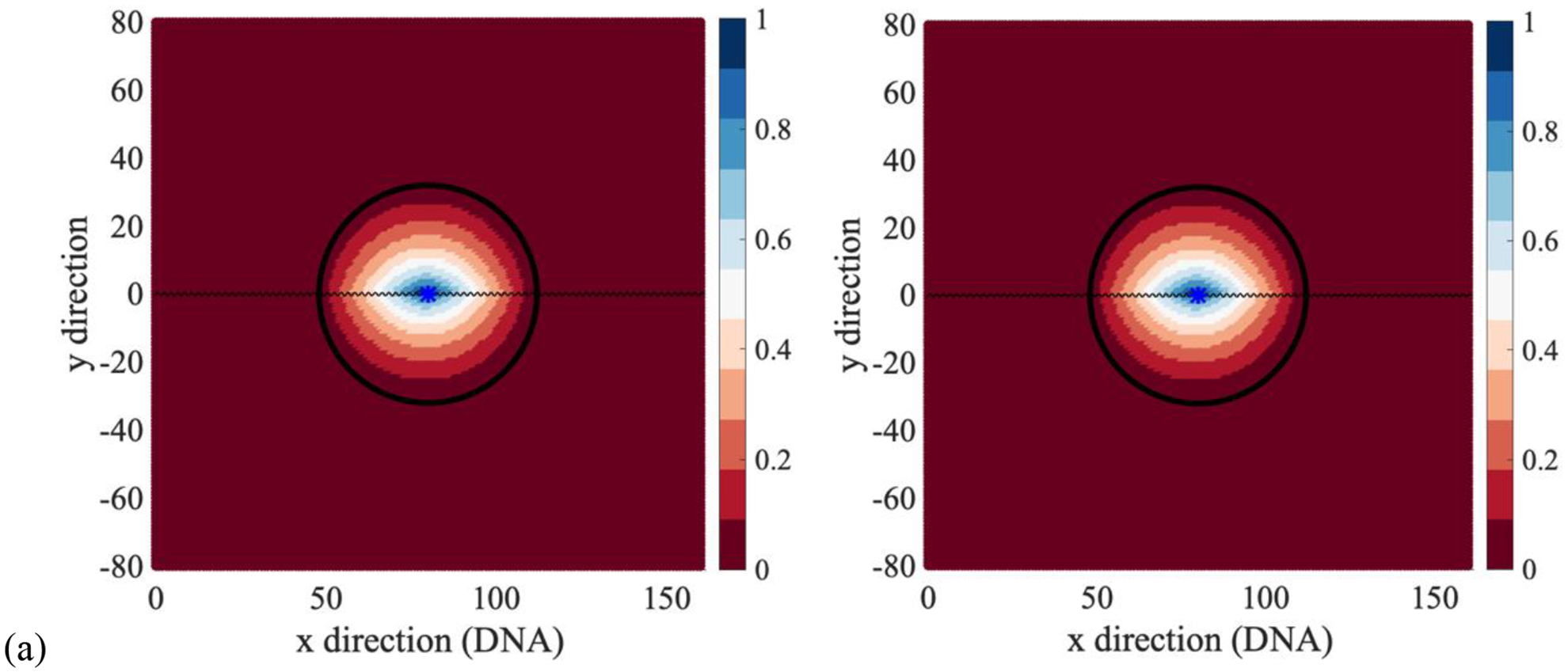
Reaction path calculations of a ligand search for a binding site on a stretched DNA molecule: (a) the committor, (b) the mean first passage time, (c) the exit time to the product. For the calculations of the committor (a) and the mean first passage time (b), the reactant R includes all the lattice points lying on or outside the circle of radius L centered at the product. The reactant lattice points are omitted in the exit time plots. The boundary between the reactant and the transition domain is a black dashed circle in the mean first passage time calculation. The product is presented by a *. The rate coefficients k_D=1 and k_off=0.01 were kept the same in all the calculations. In the figures on the left we set k_on = k_w = 10, and the right figures have k_on = k_w = 1. Hence, we vary the diffusion rates in aqueous solutions and we set the ligand binding rate equal to the rate of migration in solution.

Similar to the second example, the committor function does not change when we modify the diffusion rate in water (Fig. 9a) while the mean first passage time and ${\tau }_P^e$ change their qualitative behavior (Fig. 9b and 9c). The mean first passage time is significantly longer than the exit time to the product since the trajectories of the diffusing protein that contribute to the mean first passage time may recross the circle interfacing the reactant and the transition domain before arriving at the product; in contrast, the trajectories that contribute to the exit time to the product are always confined within the circle.

Figures 9b and 9c illustrate the impact of diffusion rates, or the rate of hopping between the lattice sites on the most efficient pathways. As we decrease the rate coefficients for transition between lattice points in aqueous solution the system is more likely to conduct an efficient search along the one-dimensional DNA. The combination of 1D and 3D diffusion are consistent with experimental observations and other theories that were discussed above.⁴³

E. THE TRANSITION STATE

One attractive feature of the committor function is that it provides a way to define a transition states as the hypersurface with the value of the committor equal 0.5.¹³ This transition state is intuitive and is hepful in the investigations of reaction mechanisms. The question we address in this section is: Can we find a corresponding definition of a transition state using the mean first passage time, or the exit times?

We define the transition function T^e (x, p) as

$${\text{T}}^e\left(x,p\right)=log\left[{\tau }_{\left(x,p\right)\to P}^e/{\tau }_{\left(x,p\right)\to R}^e\right]$$ (25)

The transition state is obtained for the set of points (x, p) such that T^e (x, p) = 0. That is, we consider the points in the transition domain that have the same exit times to both the reactant and the product states. Deviations from the transition state impact the balance between the two transition times and the value of T^e (x, p). In Figure 10 we show contour plots of the transition function for the second and third examples of this manuscript.

Figure 10.

Contour plots of the transition function T^e (x, p) for two of the examples provided in the manuscript. (A) Coordinate dependent migration (section III.B), (B) A potential with three metastable states (section III.C) with temperature of 0.25, (C) A potential with three metastable states (section III.C) with temperature of 1.0. The contour lines of T^e (x, p) = 0 are the transition states.

It is interetsing to note the similarity of the transition states as defined with the transition function equal to zero in Figure 10 and the committor function equal 0.5 in Figure 5a and 7a. Of course, the exit times include temporal information, missing from the committor, which can be exploited in other ways.

IV. DISCUSSION AND CONCLUSIONS

We have considered three functions, or reaction coordinates, that can capture and describe the progress of a molecular rearrangement, the committor, the mean first passage time and the exit time to the product. One of these functions, the committor, is often considered a “perfect” reaction coordinate. As we illustrate here, however, the committor does not include temporal information. From this perspective the committor is similar to the free energy, an analogy that is worth exploring. The free energy landscape is useful for modeling kinetics close to equilibrium and for identifying reaction bottlenecks. High free energy barriers, which the system must pass between the reactants and the products, are usually bottlenecks of reactions. The rate of transitions across the landscape, however, also depends on mobility (or, equivalently, diffusivity), which cannot be determined from the free energy. If the free energy barriers are high and the reactive trajectories are confined within a narrow tube then the diffusivity will not significantly impact the choice of the reaction coordinate. If, however, there are alternative reaction pathways with comparable barriers, or if the reaction is diffusion-controlled, then the mobility will likely influence the molecular mechanism, as illustrated here.

A similar argument applies to the committor. In the Milestoning language the committor depends only on K, the transition kernel between the milestones (Eq. 4) and not on the times of the local transitions, which are contained in the lifetime vector t. If the transition probabilities chart a unique bottleneck (a domain of low transition probability that must be traversed to reach the product) then the committor is a good measure of the reaction coordinate. If, however, there are multiple competing pathways and/or the transition times depend strongly on the milestones, the committor, as a way to identify the dominant reaction mechanism, can be misleading.

Moreover, as noted earlier, the committor function emphasizes the efficiency of product release. If we focus on early events and the onset of the reaction (e.g. in biological signaling) the fastest routes are the most significant. The identification of the fastest pathways is not addressed by the committor function.

The mean first passage time and exit time to the product (Eqs. (6) and (14)) supplement the committor by including time information (the mean first passage time was proposed as a reaction coordinate by Park et al.²⁴). The use of mean first passage time as a reaction coordinate has the advantage that it directly reports an experimental observable (specifically, the mean first passage time from the reactant to the product). The mean first passage time includes significant “incubation” time at the reactant. This is obviously a disadvantage, if we wish to focus on the transition domain, and we therefore also consider the exit time. Moreover, the exit time to the product is related to another experimental observable, the transition path time and it therefore offers a fresh view on the kinetics of the process. Several numerical examples reported here illustrate the differences between the above reaction coordinates and suggest that the committor maybe unsatisfactory when multiple competing pathways exist, the diffusivity is a significant function of the position, and when the interest is in early events of the reaction.

Modeling of reactions is greatly assisted by simulations and their analyses. The calculation of the mean first passage time, the committor, and the exit times is facilitated by the availability of enhanced sampling techniques for kinetics, such as Milestoning,²⁹ weighted ensemble,⁴⁸ and non-equilibrium umbrella sampling.⁴⁹ In particular the use of meshes in these methods makes it possible to compute the functions of the committor, mean first passage time, and the exit time on the grid. Analyzing trajectory data to depict molecular mechanisms is an important step providing both quantitative and qualitative insights. Given that different definitions of reaction coordinates are sub-optimal in different ways, in order to improve understanding of the transition it is then useful to examine alternative definitions of the reaction coordinate before settling on one mechanism and not the other.

Although different reaction coordinates may offer different qualitative views of the same process, they may be related mathematically. Here we show a formal connection between the committor, the mean first passage time, and the exit time from the domain separating the reactant from the product (Eq. (13)). This connection is particularly interesting given that the mean first passage time and the exit time are experimentally accessible, for example, via single-molecule measurements of biomolecular dynamics.

APPENDIX: The Master equation and the matrix of transition times.

Consider a system that is described by a Master equation

$$\frac{d{P}_i}{dt}=-{\sum }_j{k}_{ji}{P}_i+{\sum }_j{k}_{ij}{P}_j$$ (A.1)

In this system the time dependent transition probability from state i to state j is given by¹⁴

$$K_{ij}\left(t\right)=k_{ij}\cdot exp\left(-{\sum }_j{k}_{ij}\cdot t\right)$$ (A.2)

The probability of transition between a pair of milestones at any time (this is an element of the K matrix which is used in this paper) is given by

$$K_{ij}={\int }_0^{\infty }{K}_{ij}\left(t\right)dt=\frac{k_{ij}}{{\sum }_j{k}_{ij}}$$ (A.3)

The average transition time between milestone i and milestone j, t_ij, is

$$t_{ij}={\int }_0^{\infty }t\cdot K_{ij}\left(t\right)dt=\frac{k_{ij}}{{\left({\sum }_j{k}_{ij}\right)}^2}$$ (A.4)

Note however that the lifetime of a milestone is given by

$$t_i={\sum }_j{t}_{ij}=\frac{1}{{\sum }_j{k}_{ij}}$$ (A.5)

And we can therefore write

$$t_{ij}=K_{ij}\cdot t_i$$ (A.6)

which is the same as the matrix relationship given in section II: T = T₀K.

REFERENCES

- 1.Ulitsky A; Elber R, A new technique to calculate steepest descent paths in flexible polyatomic systems. J. Chem. Phys 1990, 92, 1510–1511. [Google Scholar]
- 2.Jonsson H; Mills G; Jacobsen KW, Nudged elastic band method for finding minimum energy paths of transitions In Classical and quantum dynamics in condensed phase simulations, Berne BJ; Ciccotti G; Coker DF, Eds. World Scientific: Singapore, 1998; pp 385–403. [Google Scholar]
- 3.Olender R; Elber R, Yet another look at the steepest descent path. J. Mol. Struct. : THEOCHEM 1997, 398, 63–71. [Google Scholar]
- 4.E WN; Ren WQ; Vanden-Eijnden E, String method for the study of rare events. Phys. Rev. B 2002, 66, 4. [DOI] [PubMed] [Google Scholar]
- 5.Templeton C; Chen SH; Fathizadeh A; Elber R, Rock climbing: A local-global algorithm to compute minimum energy and minimum free energy pathways. J. Chem. Phys 2017, 147, 10. [DOI] [PMC free article] [PubMed] [Google Scholar]
- 6.Berkowitz M; Morgan JD; McCammon JA; Northrup SH, Diffusion-controlled reactions - a variational formula for the optimum reaction coordinate. J. Chem. Phys 1983, 79, 5563–5565. [Google Scholar]
- 7.Huo SH; Straub JE, The MaxFlux algorithm for calculating variationally optimized reaction paths for conformational transitions in many body systems at finite temperature. J. Chem. Phys 1997, 107, 5000–5006. [Google Scholar]
- 8.Viswanath S; Kreuzer SM; Cardenas AE; Elber R, Analyzing milestoning networks for molecular kinetics: Definitions, algorithms, and examples. J. Chem. Phys 2013, 139, 174105. [DOI] [PMC free article] [PubMed] [Google Scholar]
- 9.Elber R; Shalloway D, Temperature dependent reaction coordinates. J. Chem. Phys 2000, 112, 5539–5545. [Google Scholar]
- 10.Faccioli P; Sega M; Pederiva F; Orland H, Dominant pathways in protein folding. Phys. Rev. Lett 2006, 97, 108101. [DOI] [PubMed] [Google Scholar]
- 11.Maragliano L; Fischer A; Vanden-Eijnden E; Ciccotti G, String method in collective variables: Minimum free energy paths and isocommittor surfaces. J. Chem. Phys 2006, 125, 024106. [DOI] [PubMed] [Google Scholar]
- 12.Ciccotti G; Kapral R; Vanden-Eijnden E, Blue moon sampling, vectorial reaction coordinates, and unbiased constrained dynamics. ChemPhysChem. 2005, 6, 1809–1814. [DOI] [PubMed] [Google Scholar]
- 13.Vanden-Eijnden E; Tal FA, Transition state theory: Variational formulation, dynamical corrections, and error estimates. J. Chem. Phys 2005, 123, 184103. [DOI] [PubMed] [Google Scholar]
- 14.Elber R; Makarov DE; Orland H, Molecular Dynamics in Condensed Phases: Theory, Simulations, and Analysis. John WIley and Sons: New Jersey, 2020. [Google Scholar]
- 15.Votapka LW; Amaro RE, Multiscale Estimation of Binding Kinetics Using Brownian Dynamics, Molecular Dynamics and Milestoning. PLoS Comput. Biol 2015, 11, e1004381. [DOI] [PMC free article] [PubMed] [Google Scholar]
- 16.Cardenas AE; Elber R, Kinetics of cytochrome C folding: Atomically detailed simulations. Proteins : Struct., Funct., Genet 2003, 51, 245–257. [DOI] [PubMed] [Google Scholar]
- 17.Onsager L, Initial recombination of ions. Phys. Rev 1938, 54, 554–557. [Google Scholar]
- 18.Peters B; Bolhuis PG; Mullen RG; Shea JE, Reaction coordinates, one-dimensional Smoluchowski equations, and a test for dynamical self-consistency. J. Chem. Phys 2013, 138, 054106. [DOI] [PubMed] [Google Scholar]
- 19.E WN; Vanden-Eijnden E, Transition-Path Theory and Path-Finding Algorithms for the Study of Rare Events In Annu. Rev. Phys. Chem, Vol 61, Leone SR; Cremer PS; Groves JT; Johnson MA; Richmond G, Eds. 2010; Vol. 61, pp 391–420. [DOI] [PubMed] [Google Scholar]
- 20.Peters B; Beckham GT; Trout BL, Extensions to the likelihood maximization approach for finding reaction coordinates. J. Chem. Phys 2007, 127, 034109. [DOI] [PubMed] [Google Scholar]
- 21.Ma A; Dinner AR, Automatic method for identifying reaction coordinates in complex systems. J. Phys. Chem. B 2005, 109, 6769–6779. [DOI] [PubMed] [Google Scholar]
- 22.Metzner P; Schutte C; Vanden-Eijnden E, Transition path theory for markov jump processes. Multiscale Model. Simul 2009, 7, 1192–1219. [Google Scholar]
- 23.Elber R; Bello-Rivas MJ; Ma P; Cardenas AE; Fathizadeh A, Calculating Iso-Committor Surfaces as Optimal Reaction Coordinates with Milestoning. Entropy 2017, 19, 219. [DOI] [PMC free article] [PubMed] [Google Scholar]
- 24.Park S; Sener MK; Lu DY; Schulten K, Reaction paths based on mean first-passage times. J. Chem. Phys 2003, 119, 1313–1319. [Google Scholar]
- 25.Chung HS; Eaton WA, Protein folding transition path times from single molecule FRET. Curr. Opin. Struct. Biol 2018, 48, 30–39. [DOI] [PMC free article] [PubMed] [Google Scholar]
- 26.Greenleaf WJ; Woodside MT; Block SM, High-resolution, single-molecule measurements of biomolecular motion. Annu. Rev. Biophys. Biomol. Struct 2007, 36, 171–190. [DOI] [PMC free article] [PubMed] [Google Scholar]
- 27.Cossio P; Hummer G; Szabo A, Transition paths in single-molecule force spectroscopy. J. Chem. Phys 2018, 148, 123309. [DOI] [PMC free article] [PubMed] [Google Scholar]
- 28.Berezhkovskii AM; Makarov DE, On the forward/backward symmetry of transition path time distributions in nonequilibrium systems. J. Chem. Phys 2019, 151, 065102. [Google Scholar]
- 29.Elber R, A new paradigm for atomically detailed simulations of kinetics in biophysical systems. Q. Rev. Biophys 2017, 50, e8. [DOI] [PubMed] [Google Scholar]
- 30.Kirmizialtin S; Elber R, Revisiting and Computing Reaction Coordinates with Directional Milestoning. J. Phys. Chem. A 2011, 115, 6137–6148. [DOI] [PMC free article] [PubMed] [Google Scholar]
- 31.Vanden Eijnden E; Venturoli M; Ciccotti G; Elber R, On the assumption underlying Milestoning. J. Chem. Phys 2008, 129, 174102. [DOI] [PMC free article] [PubMed] [Google Scholar]
- 32.Bello-Rivas JM; Elber R, Exact milestoning. J. Chem. Phys 2015, 142, 094102. [DOI] [PMC free article] [PubMed] [Google Scholar]
- 33.Aristoff D; Bello-Rivas JM; Elber R, A mathematical framework for exact milestoning. Multiscale Model. Simul 2016, 14, 301–322. [DOI] [PMC free article] [PubMed] [Google Scholar]
- 34.Hawk AT; Konda SSM; Makarov DE, Computation of transit times using the milestoning method with applications to polymer translocation. J. Chem. Phys 2013, 139, 064101. [DOI] [PubMed] [Google Scholar]
- 35.West AMA; Elber R; Shalloway D, Extending molecular dynamics time scales with milestoning: Example of complex kinetics in a solvated peptide. J. Chem. Phys 2007, 126, 145104. [DOI] [PubMed] [Google Scholar]
- 36.Stormo GD, Introduction to Protein-DNA Interatcions: Structure, Thermodynamics, and Bioinformatics. Cold Spring Harbor Laboratory Press: 2013. [Google Scholar]
- 37.Riggs AD; Bourgeois S; Cohn M, The lac-repressor-operator interaction. 3. Kinetic studies. J. Mol. Biol 1970, 53, 401–417. [DOI] [PubMed] [Google Scholar]
- 38.Richter PH; Eigen M, Diffusion controlled reaction-rates in spheroidal geometry - application to repressor-operator association and membrane-bound enzymes. Biophys. Chem 1974, 2, 255–263. [DOI] [PubMed] [Google Scholar]
- 39.Berg OG; Winter RB; Vonhippel PH, Diffusion-driven mechanisms of protein translocation on nucleic-acids .1. models and theory. Biochemistry 1981, 20, 6929–6948. [DOI] [PubMed] [Google Scholar]
- 40.Winter RB; Berg OG; Vonhippel PH, Diffusion-driven mechanisms of protein translocation on nucleic-acids .3. the escherichia-coli-lac repressor-operator interaction - kinetic measurements and conclusions. Biochemistry 1981, 20, 6961–6977. [DOI] [PubMed] [Google Scholar]
- 41.Blainey PC; van Oijent AM; Banerjee A; Verdine GL; Xie XS, A base-excision DNA-repair protein finds intrahelical lesion bases by fast sliding in contact with DNA. Proc. Natl. Acad. Sci. U. S. A 2006, 103, 5752–5757. [DOI] [PMC free article] [PubMed] [Google Scholar]
- 42.Wang YM; Austin RH; Cox EC, Single molecule measurements of repressor protein 1D diffusion on DNA. Phys.l Rev. Lett 2006, 97, 048302. [DOI] [PubMed] [Google Scholar]
- 43.Mirny L; Slutsky M; Wunderlich Z; Tafvizi A; Leith J; Kosmrlj A, How a protein searches for its site on DNA: the mechanism of facilitated diffusion. J. Phys. A: Math. Theor 2009, 42, 434013. [Google Scholar]
- 44.Hu T; Grosberg AY; Shklovskii BI, How proteins search for their specific sites on DNA: The role of DNA conformation. Biophys. J 2006, 90, 2731–2744. [DOI] [PMC free article] [PubMed] [Google Scholar]
- 45.Ando T; Skolnick J, Sliding of Proteins Non-specifically Bound to DNA: Brownian Dynamics Studies with Coarse-Grained Protein and DNA Models. PLoS Comput. Biol 2014, 10, e1003990. [DOI] [PMC free article] [PubMed] [Google Scholar]
- 46.Shin J; Kolomeisky AB, Molecular search with conformational change: One-dimensional discrete-state stochastic model. J. Chem. Phys 2018, 149, 174104. [DOI] [PubMed] [Google Scholar]
- 47.Leven I; Levy Y, Quantifying the two state facilitated diffusion model of protein-DNA interatcions. Nucleic Acids Res. 2019, 47, 5530–5538. [DOI] [PMC free article] [PubMed] [Google Scholar]
- 48.Adhikari U; Mostofian B; Copperman J; Subramanian SR; Petersen AA; Zuckerman DM, Computational Estimation of Microsecond to Second Atomistic Folding Times. J. Am. Chem. Soc 2019, 141, 6519–6526. [DOI] [PMC free article] [PubMed] [Google Scholar]
- 49.Dickson A; Maienschein-Cline M; Tovo-Dwyer A; Hammond JR; Dinner AR, Flow-Dependent Unfolding and Refolding of an RNA by Nonequilibrium Umbrella Sampling. J. Chem. Theory Comput 2011, 7, 2710–2720. [DOI] [PubMed] [Google Scholar]