Machine learning-based data analytic approaches for evaluating post-natal mouse respiratory physiological evolution

Abstract

Respiratory parameters change during post-natal development, but the nature of their changes have not been well-described. The advent of commercially available plethysmographic instruments provided improved repeatability of measurements and standardization of measured breathing in mice across laboratories. These technologies thus allowed for exploration of more precise respiratory pattern changes during the post-natal developmental epoch. Current methods to analyze respiratory behavior utilize plethysmography to acquire standing values of frequency, volume and flow at specific time points in murine maturation. These metrics have historically been independently analyzed as a function of time with no further analysis examining the interplay these variables have with each other and in the context of postnatal maturation or during blood gas homeostasis. We posit that machine learning workflows can provide deeper physiological understanding into the postnatal development of respiration. In this manuscript, we delineate a machine learning workflow based on the R-statistical programming language to examine how variation and relationships of frequency (f) and tidal volume (TV) change with respect to inspiratory and expiratory parameters. Our analytical workflows could successfully predict age and found that the variation and relationships between respiratory metrics are dynamically shifting with age and during hypercapnic breathing. Thus, our work demonstrates the utility of high dimensional analyses to provide reliable class label predictions using non-invasive respiratory metrics. These approaches may be useful in large-scale phenotyping across development and in disease.

1. Introduction

Unlike other parts of the brain where neural networks require a learned input to generate mature circuits, the autonomic nervous system requires connections to be generated and reinforced during development, so that the animal may properly interact with the ex utero environment following birth. Nevertheless, significant changes in brain circuitry have been reported during postnatal development. For instance, the post-natal developmental epoch shows significant “connectomic” changes in the area postrema (Gokozan et al., 2016) and pre-Bötzinger complex (Mei-Ling Liu et al., 2018), indicating that vital system homeostasis shows developmentally dynamic behavior during postnatal growth. Both prior and after birth, respiratory regulation evolves to refine breathing control under normoxic normocapnic conditions, as well as during physiological changes in blood gases such as that experienced when exogenous hypoxia or hypercapnia are administered (Jansen and Chernick, 1983). This evolution involves not only the postnatal development of discrete cellular populations involved with breathing, but also the integration of peripheral sensory input from the carotid bodies (Carroll and Kim, 2005) and the respiratory network distributed throughout the medulla and pons (Alheid et al., 2004). Failure to appropriately develop and integrate these aspects may lead to the dysregulation of breathing and underlie the pathophysiology in diseases such as Sudden Infant Death Syndrome (SIDS), Congenital Central Hypoventilation Syndrome and sleep apnea. Thus, the potential to isolate subtle but relevant changes in respiratory phenotype using high dimensionality datasets of autonomic functions with non-invasive techniques offers a potential avenue for screening human pathologies with autonomic dysfunction.

The regulation of breathing involves the coordination of self-oscillating brainstem networks. These include the pre-Bötzinger complex, the parafacial respiratory group and the post-inspiratory complex (Smith et al., 1991; Feldman and Del Negro, 2006; Anderson et al., 2016, and recently reviewed by (Del Negro et al., 2018)). Identification of neural circuits has been largely investigated through electrophysiological recordings of brain slice preparations, but genetic lineage tracing has increased our understanding of how these circuits develop (Gray, 2013; Rose et al., 2009a, b; Tupal et al., 2014; van der Heijden and Zoghbi, 2020; Wang et al., 2005). Although significant effort to characterize the neuron populations and firing behaviors of respiratory drivers exist, the post-natal developmental evolution of respiratory maturation continues to be a significant knowledge gap in autonomic developmental neuroscience.

Current methods to investigate post-natal developmental changes using in vivo experimental respiration paradigms typically perturb specific neuronal populations within the brainstem to characterize the effects produced on respiration. Optogenetic stimulation of Dbx1-interneuron populations in the pre-Bötzinger complex significantly modulates respiratory frequency (Vann et al., 2018). Similarly, Dosumu-Johnson et al., 2018 showed that acute disturbances in serotonergic Pet1-neuron activity directly inhibits apneic recovery positing that such cardiorespiratory decoupling may underlie a subset of SIDS etiologies. Furthermore, Phox2b-expressing neurons mediate many aspects of central chemosensation which is influenced via neuronal and astrocytic cell populations within the brain stem (Czeisler et al., 2019; Hawkins et al., 2017; Moreira et al., 2016; Sobrinho et al., 2017). The wide commercial availability of plethysmographic tools for neonatal mouse pup recordings permits the recording of mouse pup respiratory pattern evolution in vivo, making possible the ability to explore how integrated respiration occurs in live animals over the post-natal developmental period. Through these instruments, real time breathing can be quantified by placing animals into specialized chambers which evaluate air volume changes and other breathing parameters through standardized approaches (Chapin, 1954; Drorbaugh and Fenn, 1955; Mortola and Frappell, 2013; Lim et al., 2014). While the tool has been largely evaluated for reliability and characterization of raw breathing differences between age, past analytic tools were unable to evaluate the differences in plethysmography tracings in an integrated fashion that reflects the brainstem networks that underlie these paradigms and separate these differences from predicted changes in breathing as a function of developmental growth or body mass (Flandre et al., 2003; Onodera et al., 1997). However, more recently in the clinical realm, machine learning has arisen as a tool to predict lung and cardiac function based on measurements made from plethysmographic tools (Gawlitza et al., 2019; Pereira et al., 2019). Applying these similar methodologies, machine learning based pipelines can be used to not only evaluate raw read tracings to explore developmental changes of breathing over time, but more deeply evaluate the characteristics of breathing that shift.

Utilizing a R-based statistical workflow to analyze in vivo plethysmography data obtained from developing mice pups, we developed statistical models of breathing frequency (f) and tidal volume (TV). Additionally, we elucidated underlying changes in parameter variation within mice and discovered subtle relationships that would have been missed using status quo analytical workflows. We identified the principal respiratory parameters that change with time by training machine learning algorithms to determine the extent to which age could be accurately predicted based on (i) features of respiratory linear models and (ii) features describing breathing variation. These workflows represent objective methods to quantify changes in breathing and demonstrate that the features of breathing variation and the relationships these features have dynamically evolve during post-natal development.

2. Material and methods

2.1. Experimental animals and animal husbandry

Procedures utilizing mice were performed in accordance to The Ohio State University Institutional Animal Care and Use Committee guidelines (Protocol number: 2012A00000162-R1). Animals were utilized following The Ohio State University Institutional Animal Care and Use Committee guidelines. These secondary analyses of plethysmographic data were extracted from a previously published dataset (Alzate-Correa et al., 2020) obtained from our lab stock of C57/blc6 mice at ages: P1 (n = 9), P21 (n = 8 for baseline analysis, n = 8 for hypercapnia analysis), and P56 (n = 9 for baseline, n = 9 for hypercapnia).

2.2. Plethysmography analysis in mice

Respiration was analyzed in neonatal pups using a mouse pup whole-body plethysmography chamber (#987365, DSI) and QT preamplifier (#894002, DSI). P1 pups were placed in the chamber in the head-out configuration and acclimated for 1 min before respiration was recorded for 10 min. Breathing in adult mice was monitored using a whole-body plethysmographer (#992541, DSI) with the Buxco Finepointe 2-site controller (#993582, DSI). Finepointe software was used (v2.4.7.10175) to record the following respiratory parameters: respiratory frequency (f, breaths per minute), tidal volume (TV, mL), resting time between breaths (Tr, sec), inspiratory time (Ti, sec), expiratory time (Te, seconds), peak inspiratory flow (PIF, mL per sec) and peak expiratory flow (PEF, mL per sec). P21 and P56 animals also experienced chemoreflex analysis under plethysmography. Plethysmograph acclimatization occurred by filling the chamber with room air for 30 min a day for 3 consecutive days. On the day of recording each mouse underwent acclimatization to the chamber filled with room air for 5 min, followed by baseline recordings for 20 min. For chemoreflex analysis, responses to hypercapnia (7 % CO₂) were recorded for 10 min. Only data from the baseline and CO₂ phases were evaluated in this study. No hypercapnic breathing data is recorded for P1 mice as the hypercapnic chamber could not be used on mice from this age group.

2.3. Data processing and analysis

Full baseline and hypercapnic recordings were analyzed and raw respiratory data was first standardized by body mass and analyzed in R. These parameters were used to generate linear models of mice breathing frequency (f) and tidal volume (TV) as factors of both inspiratory and expiratory breathing. Pearson correlation coefficients were calculated and visualized using ggplot2 (Wickham, 2016) to identify potential relationships of f and TV to other breathing parameters including PIF, PEF, Ti, Te and Tr. Poincaré variation plots were created utilizing the above-mentioned data with custom code and the car package (Fox and Weisberg, 2011) and ggplot2 package in R. Utilizing the features generated from our linear models and Poincaré plots, data frames were built with each row representing individual animals and each column representing a feature. Data frames were then centered and scaled prior to analysis utilizing the ‘scale’ function in R’s base package. Principal component analysis (PCA) and linear discriminate analysis (LDA) were performed utilizing unique scripts and the MASS package (Venables and Ripley, 2002), and visualized using ggplot2 packages within R to identify data clustering. This was compared against kmeans cluster analysis found with the ‘kmeans’ function in R’s base package and visualized using the factoextra package (Kassambara and Mundt, 2020). Feature detection was done utilizing the Boruta package (Kursa and Rudnicki, 2010). Machine learning algorithms were implemented utilizing the caret (Kuhn, 2008; Kuhn et al., 2020), e1071 (Meyer et al., 2019), and randomForest (Liaw and Wiener, 2002) packages in R. Random forest algorithms were built by randomly subsetting 60 % of the data set as training and 40 % as test data within the randomForest package. Implemented formulas were based upon the non-rejected feature selection in Boruta. Similarly, gradient boosted algorithms were built with matching features and datasets within the caret package. Finally, support vector machines were built utilizing the ‘svm’ function in e1071. All code used to perform the analyses are located in the supplemental materials or can be found at https://github.com/WesleyWang913/Wang-et-al-2020-Code-Supplement.

3. Results

3.1. Summary of data analytical workflow procedures

The ML/AI toolbox has a diverse set of instruments that can be used in various settings, with no methodology being necessarily supreme to others. Our general approach to evaluating neurophysiology datapoints typically begins with strong data preservation procedures such as maintaining raw data on backup servers. We next use interactive data visualization to identify trends and explore relationships between variables and identify redundancies in measurements. We then typically employ clustering algorithms to identify clustering trends, and utilize class-label prediction tools to identify principal drivers of such clusters. We hope that this manuscript may serve as a rubric for others to apply such techniques to their own research.

3.2. Respiratory breathing feature relationships shift with age and breathing gas

As evidenced in Fig. 1 Panels A–C, P1 mice frequency and tidal volume are smaller, while respiration time is greater when compared with aged counterparts. However, at more advanced ages (P21 and P56) the differences lessen during normal breathing and in hypercapnic breathing. Nevertheless, when looking at the relationships of these parameters it can be seen that at P1 the relationship of f and TV to Ti varies from that of P21 and P56. Moreover, under hypercapnic breathing a consolidation of these parameters becomes visible when compared to their age matched baseline counterparts (Fig. 1, D&E).

Fig. 1. Standing breathing parameters cannot elucidate ages further in development.

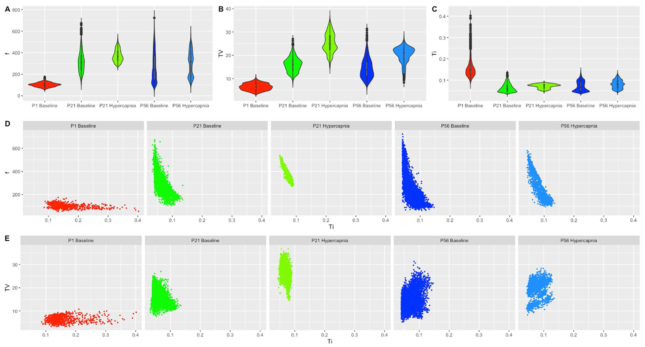
Violin plots of (A) breathing frequency (breaths/min), (B) tidal volume (mL/kg) (C) inspiratory time (sec) were generated in ggplot2 for P1 baseline breathing, P21 baseline breathing, P21 hypercapnic breathing, P56 baseline breathing and P56 hypercapnic breathing. Inspiratory time was then plotted as a relationship on the x-axis to either (D) breathing frequency on the y-axis or (E) tidal volume on the y-axis. All variables were plotted in the same x and y scale to appreciate data dispersion and shape. P1 hypercapnia was not included as mice could not be measured in the hypercapnic chamber.

Exploring how the relationships among various respiratory parameters changed during post-natal development and under challenged breathing states, we studied correlations between variables at baseline room air and at hypercapnic challenge (note that P1 studies lack hypercapnic chemoreflex data as breathing from P1 mice could not be measured in the hypercapnic breathing chamber available). At P1, f shows positive correlations with flow rates (PIF and PEF) and negative relationships with breathing times (Ti, Te and Tr). However, while the relationship of f to breathing times began to strengthen when developmental age increased, the relationship to flow rates initially strengthened at P21 and then weakened at P56. With respect of f to TV, P1 pup frequency showed no correlation to TV, a weakly positive correlation to TV at P21, and a weakly negative correlation at P56 (Fig. 2, A–C). Similarly to f, TV correlation with PIF and PEF was weakly positive at P1 and increased at P21, but at P56 PIF had weakened while PEF strengthened. In contrast, TV had a little correlation with breathing times at P1, weakly negative correlation at P21, and positive correlations at P56 (Fig. 2, A–C). Looking further at hypercapnia in comparison to age-matched baseline, while relationships of flow and breathing times to f were in the same positive or negative direction at baseline, animals experienced a prominent strengthening of these relationships under hypercapnia (Fig. 2, B–E). Flow and breathing times relationship to TV in contrast showed moderated strengthening in P21 mice and weakening in P56 mice (Fig. 2, B–E). With these distinct relationships, we posit that linear models for f and TV can be utilized to reveal how relationships between parameters change with age and breathing gas.

Fig. 2. Relationships of frequency (f) and Tidal Volume (TV) to parameters strengthens with age and stress.

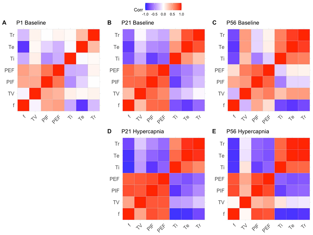
Correlation plots were generated utilizing the correlation plot function in ggplot in R. Groups are divided between ages P1, P21 and P56 and between baseline breathing (A–C) and hypercapnic breathing conditions (D–E). Red relationships represent directly proportional relationships, while blue relationships represent inversely proportional relationships. Parameters are presented as f (frequency), TV (tidal volume), PIF (peak inspiratory flow), PEF (peak expiratory flow), Ti (inspiration time), Te (expiration time) and Tr (relaxation time).

3.3. Respiratory physiology parameter variability varies with postnatal mouse ages

In addition to parameter correlation, we evaluated the extent to which respiratory parameter variability changed as a function of age and breathing gas. Although sample entropy and approximate entropy have been used to identify variability in physiological time series data (Delgado-Bonal and Marshak, 2019), their metrics are highly sensitive to the shorter biological time series datasets commonly utilized in respiratory plethysmography (Yentes et al., 2013). We therefore utilized a more traditional metric, the Poincaré plot, to visualize variability. Poincaré plots were generated to visualize the correlation between two consecutive data points in a time-series (i.e., x-axis: A_n versus y-axis: A_n+1) to measure respiratory variability (Mellen et al., 2003). Thus in the context of breathing, two consecutive breaths were evaluated such that instantaneous breathing was determined and each individual breath represents a data paint. To objectively quantify variability, we utilized two computational approaches. First, points furthest from the center (mean) were used to create a polygon; this polygon’s area quantitatively defines the deviation of the data using a convex hull operation in R. Next, a confidence ellipse containing one standard deviation of units from the mean was plotted to calculate ellipse area. These plots were all generated for each respiratory parameter in Figs. 3–9.

Fig. 3. Respiratory frequency (breaths/min) variation shows changes with age and breathing state.

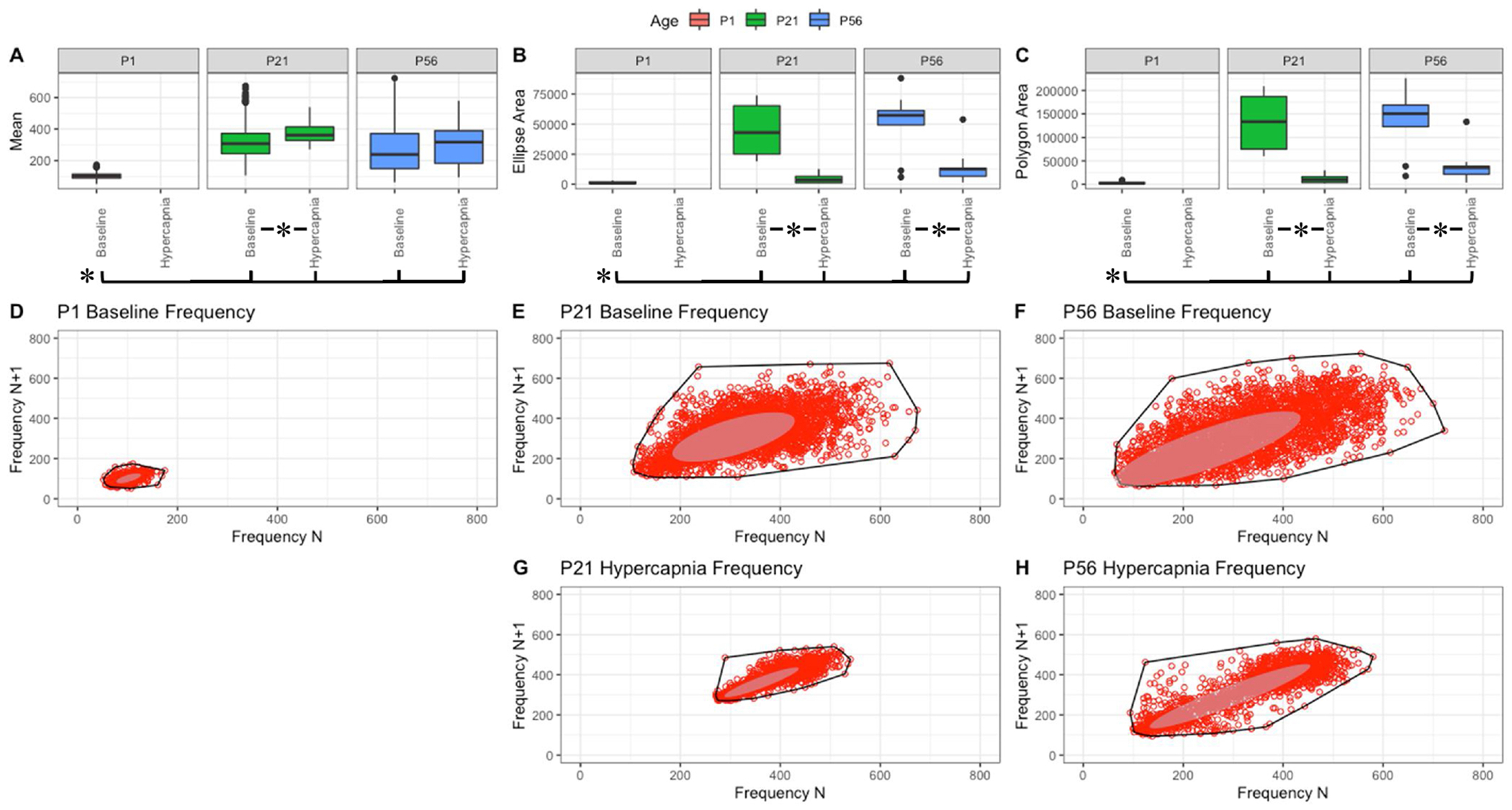
Parameter boxplots were generated to compare parameter mean (A), ellipse area (B) and polygon area (C) in P1, P21 and P56 in both baseline and hypercapnic states. P1 hypercapnia was omitted as previously mentioned in Fig. 1. Ellipse area was plotted as a confidence ellipse where center represents the mean and the outer diameter contains 1 standard deviation of the dataset. Polygon areas were generated utilizing the extreme points which form the outer margin of each plot. Poincaré plots were generated from baseline breathing states (D–F) and hypercapnic states (G–H) to visualize variation in frequency (f). T-tests were performed between age groups and breathing states for mean, polygon area and ellipse area. Bars and asterisks were utilized to represent significant variation between groups with p-values < 0.05.

Fig. 9. Respiratory relaxation time (sec) variation shows changes with age and breathing state.

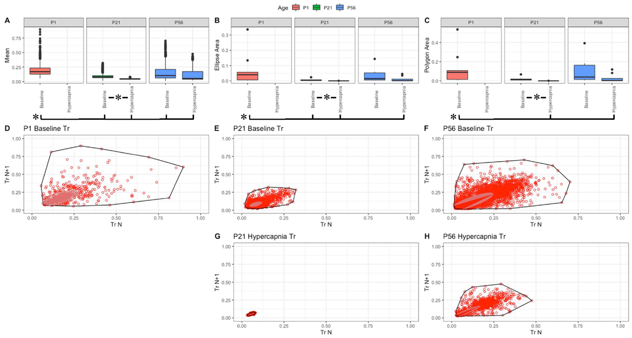
Parameter boxplots were generated to compare parameter mean (A), ellipse area (B) and polygon area (C) in P1, P21 and P56 in both baseline and hypercapnic states. P1 hypercapnia was omitted as previously mentioned in Fig. 1. Ellipse area was plotted as a confidence ellipse where center was the mean and the outer diameter contains 1 standard deviation of the dataset. Polygon areas were generated utilizing the extreme points which form the outer margin of each plot. Poincaré plots were generated from baseline breathing states (D–F) and hypercapnic states (G–H) to visualize variation in relaxation time (Tr). T-tests were performed between age groups and breathing states for mean, polygon area and ellipse area. Bars and asterisks were utilized to represent significant variation between groups with p-values < 0.05.

Within these figures, variation in f, TV, PIF and PEF changed with age as P1 parameters distinctly varied in both polygon and ellipse area (Figs. 3–6, B&C). Note that mean f is significantly smaller in P1 mice, and therefore their variance is somewhat constrained (Fig. 3, A). In the older animals, a broader variance was noted at baseline, and both showed significant reduction in variance as a response to hypercapnic challenge (Fig. 3, B&C). Compared to f, the decrease in variance in response to hypercapnic challenge was not as drastic in TV (compare Fig. 4, B&C to Fig. 3, B&C). Relative to P1, the variability parameters of the Poincaré plots to flow showed significantly more variation with increased post-natal age (Figs. 5 and 6). A different trend was noted with Ti, Te, and Tr. In baseline room air, P1 pups showed significantly more variability in Ti, Te, and Tr relative to older animals (Figs. 7–9, A–C). These finding thus suggest that respiratory parameter variation changes significantly with age as variability often increases with age and variability decreases under hypercapnic breathing states.

Fig. 6. Respiratory peak expiratoiy flow (mL/sec) variation shows changes with age and breathing state.

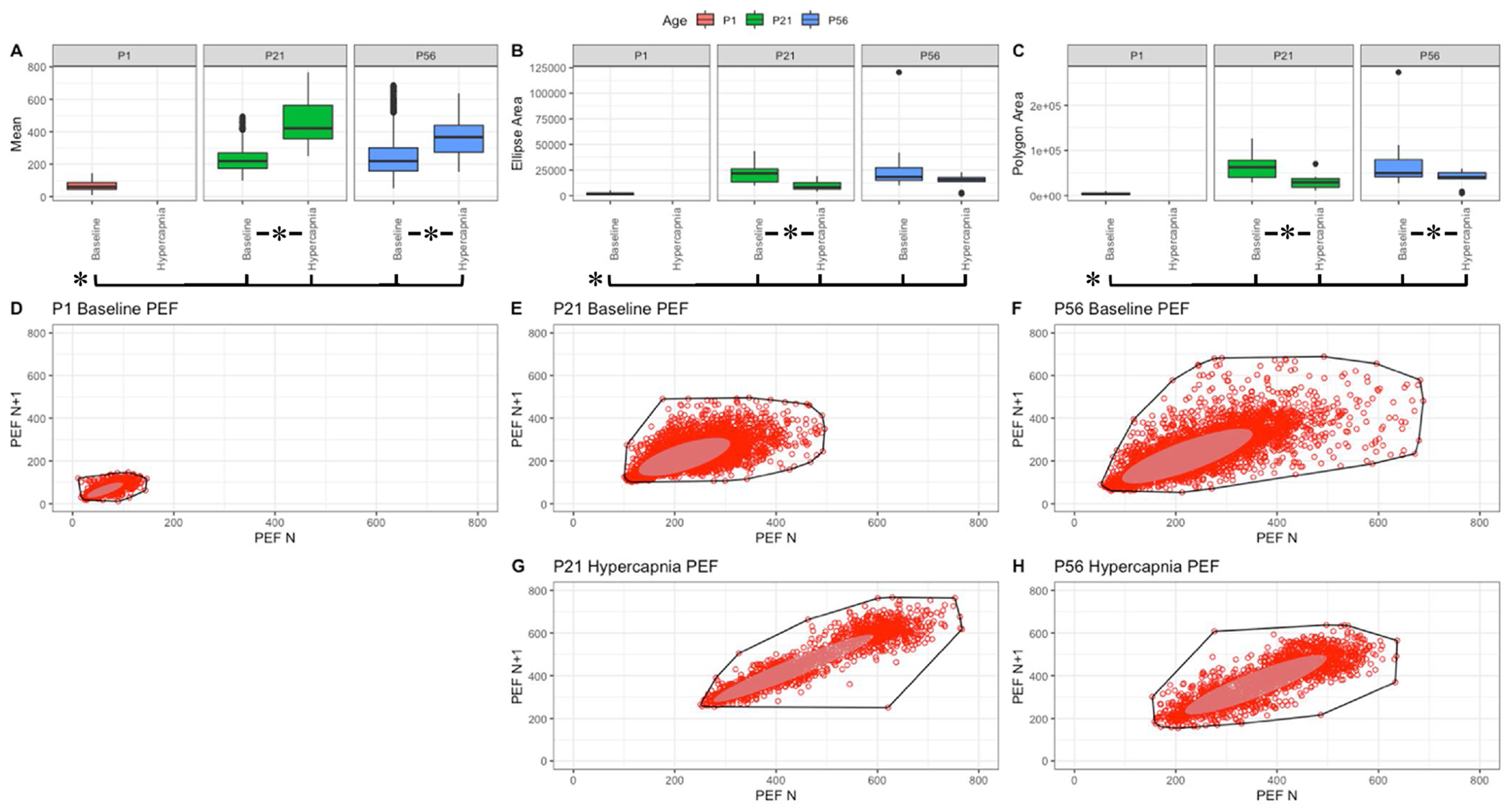
Parameter boxplots were generated to compare parameter mean (A), ellipse area (B) and polygon area (C) in P1, P21 and P56 in both baseline and hypercapnic states. P1 hypercapnia was omitted as previously mentioned in Fig. 1. Ellipse area was plotted as a confidence ellipse where center was the mean and the outer diameter contains 1 standard deviation of the dataset. Polygon areas were generated utilizing the extreme points which form the outer margin of each plot. Poincaré plots were generated from baseline breathing states (D–F) and hypercapnic states (G–H) to visualize variation in peak expiratory flow (PEF). T-tests were performed between age groups and breathing states for mean, polygon area and ellipse area. Bars and asterisks were utilized to represent significant variation between groups with p-values < 0.05.

Fig. 4. Respiratory tidal volume (mL/kg) variation shows changes with age and breathing state.

Parameter boxplots were generated to compare parameter mean (A), ellipse area (B) and polygon area (C) in PI, P21 and P56 in both baseline and hypercapnic states. P1 hypercapnia was omitted as previously mentioned in Fig. 1. Ellipse area was plotted as a confidence ellipse where center was the mean and the outer diameter contains 1 standard deviation of the dataset. Polygon areas were generated utilizing the extreme points which form the outer margin of each plot. Poincaré plots were generated from baseline breathing states (D–F) and hypercapnic states (G–H) to visualize variation in tidal volume (TV). T-tests were performed between age groups and breathing states for mean, polygon area and ellipse area. Bars and asterisks were utilized to represent significant variation between groups with p-values < 0.05.

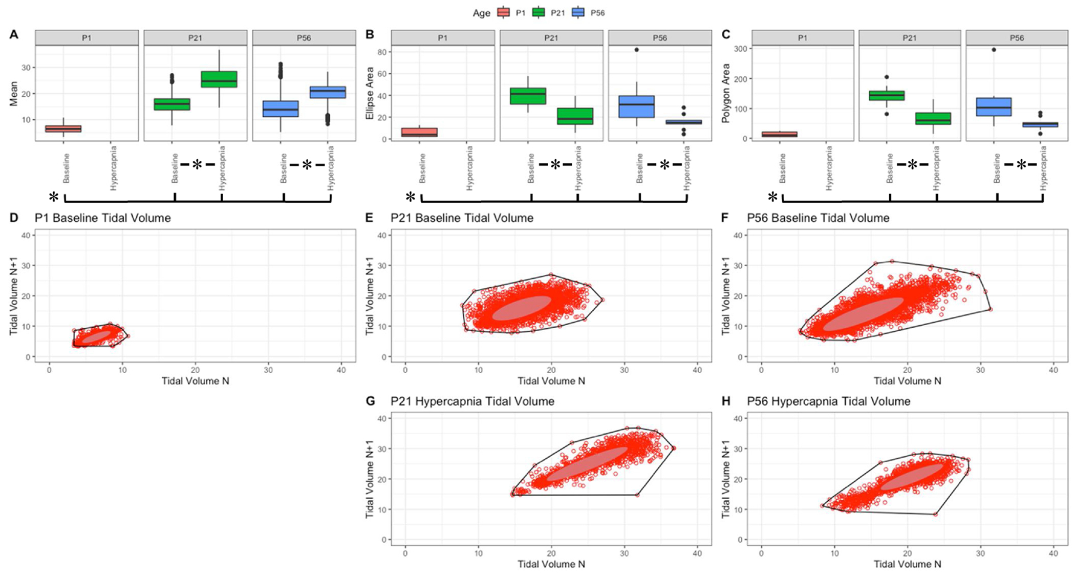
Fig. 5. Respiratory peak inspiratoiy flow (mL/sec) variation shows changes with age and breathing state.

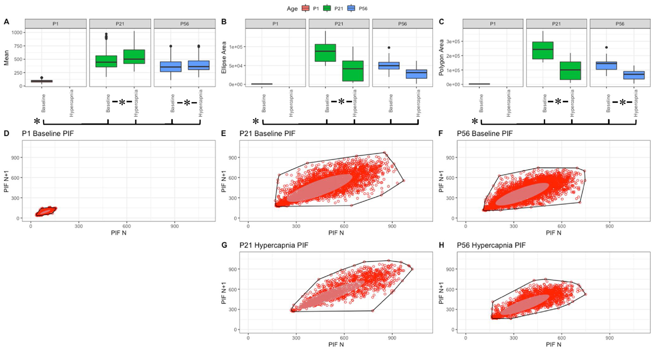
Parameter boxplots were generated to compare parameter mean (A), ellipse area (B) and polygon area (C) in P1, P21 and P56 in both baseline and hypercapnic states. P1 hypercapnia was omitted as previously mentioned in Fig. 1. Ellipse area was plotted as a confidence ellipse where center was the mean and the outer diameter contains 1 standard deviation of the dataset. Polygon areas were generated utilizing the extreme points which form the outer margin of each plot. Poincaré plots were generated from baseline breathing states (D–F) and hypercapnic states (G–H) to visualize variation in peak inspiratory flow (PIF). T-tests were performed between age groups and breathing states for mean, polygon area and ellipse area. Bars and asterisks were utilized to represent significant variation between groups with p-values < 0.05.

Fig. 7. Respiratory inspiratory time (sec) variation shows changes with age and breathing state.

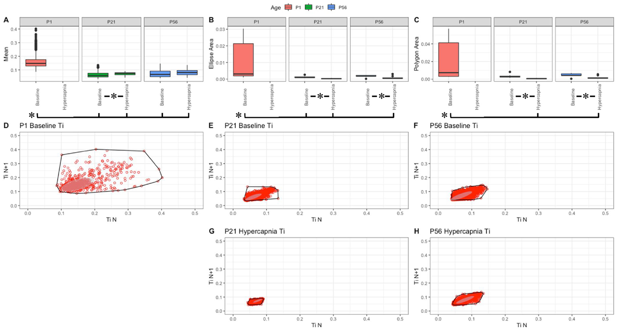
Parameter boxplots were generated to compare parameter mean (A), ellipse area (B) and polygon area (C) in P1, P21 and P56 in both baseline and hypercapnic states. P1 hypercapnia was omitted as previously mentioned in Fig. 1. Ellipse area was plotted as a confidence ellipse where center was the mean and the outer diameter contains 1 standard deviation of the dataset. Polygon areas were generated utilizing the extreme points which form the outer margin of each plot. Poincaré plots were generated from baseline breathing states (D–F) and hypercapnic states (G–H) to visualize variation in inspiratory time (Ti). T-tests were performed between age groups and breathing states for mean, polygon area and ellipse area. Bars and asterisks were utilized to represent significant variation between groups with p-values < 0.05.

3.4. Poincaré plot variation value is influenced by parameter means between ages

Mice with different biological ages show differences in raw ventilation due to body size variation during postnatal growth. Note that P1 mice were shown to have reduced means in f, TV, PIF and PEF and increased means in Ti, Te and Tr (Figs. 3–9, A). While variation was distinct amongst age it was important to address the limitations of the Poincaré plot. We achieved this by performing simple in silico simulations of Poincaré plots. Within R, functions were created that randomly generated 100 values that centered around a machine generated mean and standard deviation (SD) in order to create a data-set of variation which can be used to calculate polygon area and ellipse area. These methods were repeated for values of SD ranging from 1 to 100 and mean ranging 1–100. In turn, each simulation contained an arithmetic mean, SD, polygon area, and ellipse area.

We then performed a linear regression model in R to evaluate the relationships, and then plotted the relative influence of arithmetic mean and SD for both the polygon and ellipse area. Influence of these parameters were visualized utilizing a bubble plot where polygon area value correlated to the aesthetic size, y-axis denoted simulated standard deviation, and x-axis denoted simulated arithmetic mean (Fig. 10, A&B). Although the SD showed similar influence on polygon and ellipse area estimations, we observed that a small, yet significant influence of mean is contributed to the Poincaré scatter plot pattern based on results from the linear regression (Fig. 10, C, also note that the aesthetic area is highly increased in Fig. 10, A&B as values move in the positive y-axis direction). Thus, variation as a function of polygon and ellipse area required normalization against respiratory parameter means. We therefore derived a new metric we refer to as Respiratory Variation, being defined as corrected polygon or ellipse area– where total values of the polygon or ellipse were subtracted by the parameters means for each animal multiplied by the calculated coefficient of 82.358 and 36.543 for polygon and ellipse formulas respectively.

Fig. 10. Poincare plots are influenced by mean.

Bubble plots were created to visualize changes in mean and SD’s effects on area—represented as bubble size in the ellipse area plot (A) and polygon area plot (B). Custom R scripts were generated to calculate the relative influence both mean and SD play in affecting either the ellipse area or polygon area derived from the Poincaré plots (C).

$$\begin{gathered} {\text{Var}}_{\text{RP}}={\text{Area}}_{\text{P}}-\text{mean}\ast \text{82}.358 \\ {\text{Var}}_{\text{RE}}={\text{Area}}_{\text{E}}-\text{mean}\ast 36.543 \end{gathered}$$

These coefficients were derived from linear models of polygon and ellipse area to mean and standard deviation within R (Supplementary Materials). Using this formula, we obtained the variation score which was utilized as a feature in the subsequent machine learning workflows.

3.5. Variation and model fit of breathing parameters are drivers of differentiating age

Having identified changes in respiratory variation using the Poincaré plot method, we further explored the differences in respiratory parameters during postnatal development. To this end, we constructed a data table where animal age (P1, P21 and P56) represented the observation’s class label. Each observation’s parameters included the extracted coefficients linear models of frequency and tidal volume, the respective p-value and r-squared values of their linear regression models, and the Respiratory Variation metrics derived from the Poincaré analyses. These values were then center scaled to ease comparability amongst variables. To explore the general behavior of the data across all ages, we subsetted the data table to exclude the class labels resulting in a new data table holding only the numerical values indicated above. We then explored the data by visualizing the eigenvectors of the principal component analysis (PCA). Fig. 11 demonstrates our eigenvector plots: each eigenvector is plotted along PC1 and PC2, with its influence color coded. In all of the analyses plotted in Fig. 11, aspects of Respiratory Variation highly influenced the variance in the datasets.

Fig. 11. Variation, model coefficients and fit are drivers of age discrimination.

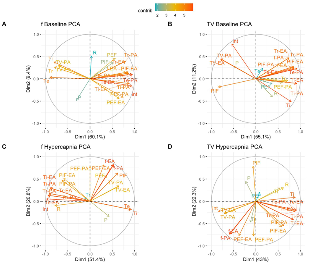
Linear model coefficients for frequency (f), tidal volume (TV), peak inspiratory flow (PIF), peak expiratory flow (PEF), inspiratory time (Ti), expiratory time (Te) and relaxation time (Tr), linear model p-value (P) and R-squared (R) values were extracted from individually modeled animals. Polygon area-derived respiratoiy variation for frequency (f-PA), tidal volume (TV-PA), peak inspiratory flow (PIF-PA), peak expiratory flow (PEF-PA), inspiratory time (Ti-PA), expiratory time (Te-PA) and relaxation time (Tr-PA) and ellipse area-derived respiratory variation for frequency (f-EA), tidal volume (TV-EA), peak inspiratory flow (PIF-EA), peak expiratory flow (PEF-EA), inspiratory time (Ti-EA), expiratory time (Te-EA) and relaxation time (Tr-EA) were additionally extracted and corrected utilizing a mean based correction factor in R. Principal component analysis (PCA) plots were utilized to highlight if specific factors may drive variation between P1, P21 and P56 mice in baseline breathing (A–B) and P21 and P56 mice in hypercapnia (C–D). P1 hypercapnia mice were omitted as mice could not be placed in the hypercapnic chamber.

After understanding and exploring the key drivers in the dataset, we next performed a supervised dimensionality reduction technique where the pup age were designated class labels for each observation and a linear discriminate analysis (LDA) was executed. In our LDA model plotted in Fig. 12 Panels A&B, baseline P1 mice visually clustered differently from adult P21 and P56 mice across the LD1 axis. Note that LD1 contributes to 98.25 % and 98.69 % for f and TV separation, respectively, and that LD2 represents 1.75 % and 1.31 % for f and TV separation, respectively. These data indicate that P1 mice are more different from P21 and P56 then P21 and P56 groups are to each other. Furthermore, hypercapnic P21 and P56 could be split along the LD1 axis (note that all data falls in the LD1 axis as only two age categories exist in hypercapnia) (Fig. 12, C&D). Thus, P1, P21, and P56 mice show significant differences in the relationships between respiratory parameters at baseline room air, and similar relationship differences were observed for P21 and P56 animals during hypercapnic challenge. In turn, LDA analyses appeared to strongly discriminate age as intuitive visual clustering was evident.

Fig. 12. Extracted parameters strongly drive the ability to discriminate age.

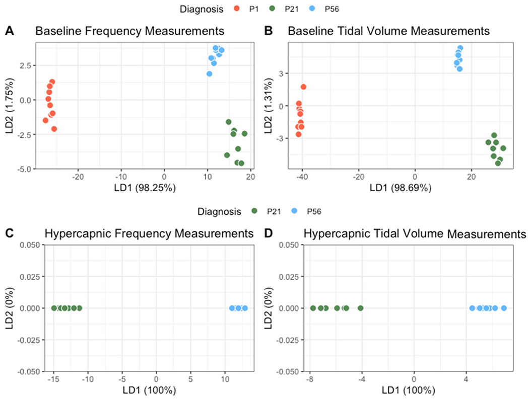
Linear discriminate analysis (LDA) plots were generated to visualize the ability to discriminate individual mice by age utilizing the extracted parameters previously described. Baseline breathing among P1, P21 and P56 (A–B) and hypercapnic breathing between P21 and P56 (C–D) are shown. All mice were clustered based upon features derived from model coefficients in relationship to frequency (A/C) or tidal volume (B/D), model fit (p-value) and variation of parameters.

To determine if such clustering could be identified in an unbiased fashion using a machine learning workflow, we utilized the kmeans cluster algorithm to identify clusters independent of the animal age label. Clusters were defined through the algorithm by identifying center points and segmenting surrounding points near the region as a cluster. Utilizing the gap statistic method to select the optimal number of clusters, it was found the optimal cluster count matched the three age categories (Fig. 13, E–H). As can be seen in Fig. 13 Panels A–D, kmeans derived clusters match age labeled clusters from the LDA plots from Fig. 12. These data suggest that by utilizing respiratory parameter relationships and variation, datasets can be stratified into distinct groups that reflect their age without providing the ground truth age, supporting the notion that machine learning algorithms can predict age.

Fig. 13. Animals cluster based on parameter relationships and respiratory variations.

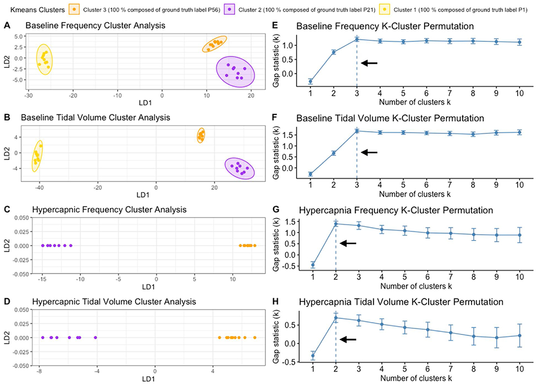
Kmeans cluster analysis was performed in R to create distinct clusters of animals independent of age labels to confirm if animals would cluster based on respiratory relationships and variation independent of age. Similar to LDA plots, baseline breathing among P1, P21 and P56 (A–B) and hypercapnic breathing between P21 and P56 (C–D) are shown with machine calculated clusters highlighted into 3/2 groups. Gap statistic analysis (E–H) was used to find the optimal number of clusters for each respective kmeans cluster analysis (A/E; B/F; C/G; D/H). Arrows indicate the optimal cluster number that was used for each plot.

Utilizing these analyzed parameters, we then defined these measures as features that can be utilized by machine learning algorithms to arrive at classification. Our next goal was to identify which features were most critical to classification. We therefore passed the features through the Boruta algorithm package within R which scrambles feature data sets at random to create a shadow feature against their non-randomized features. Features were then tested of their contribution in differentiating age against their shadow feature with features in red failing to outperform their randomized shadow features, features in yellow representing indeterminate scores, and features in green outperforming their randomized shadow feature. Features that failed to outperform their shadow feature were removed in the final features utilized in our machine learning algorithms. In baseline Boruta tests of frequency and tidal volume models, parameter variation of f, TV, PIF, PEF and Ti were valuable for age differentiation. Additionally, Te and Ti coefficients were valuable in frequency and tidal volume models respectively (Fig. 14, A&B). In contrast in hypercapnic models, parameter variation of f, TV and PEF were valuable in both frequency and tidal volume models while r-squared of the model and coefficients of PIF and Tr were valuable to frequency and tidal volume models respectively (Fig. 14, C&D).

Fig. 14. Boruta plots indicate variation and model fit are strong drivers in baseline breathing and variation is a primary driver in hypercapnia.

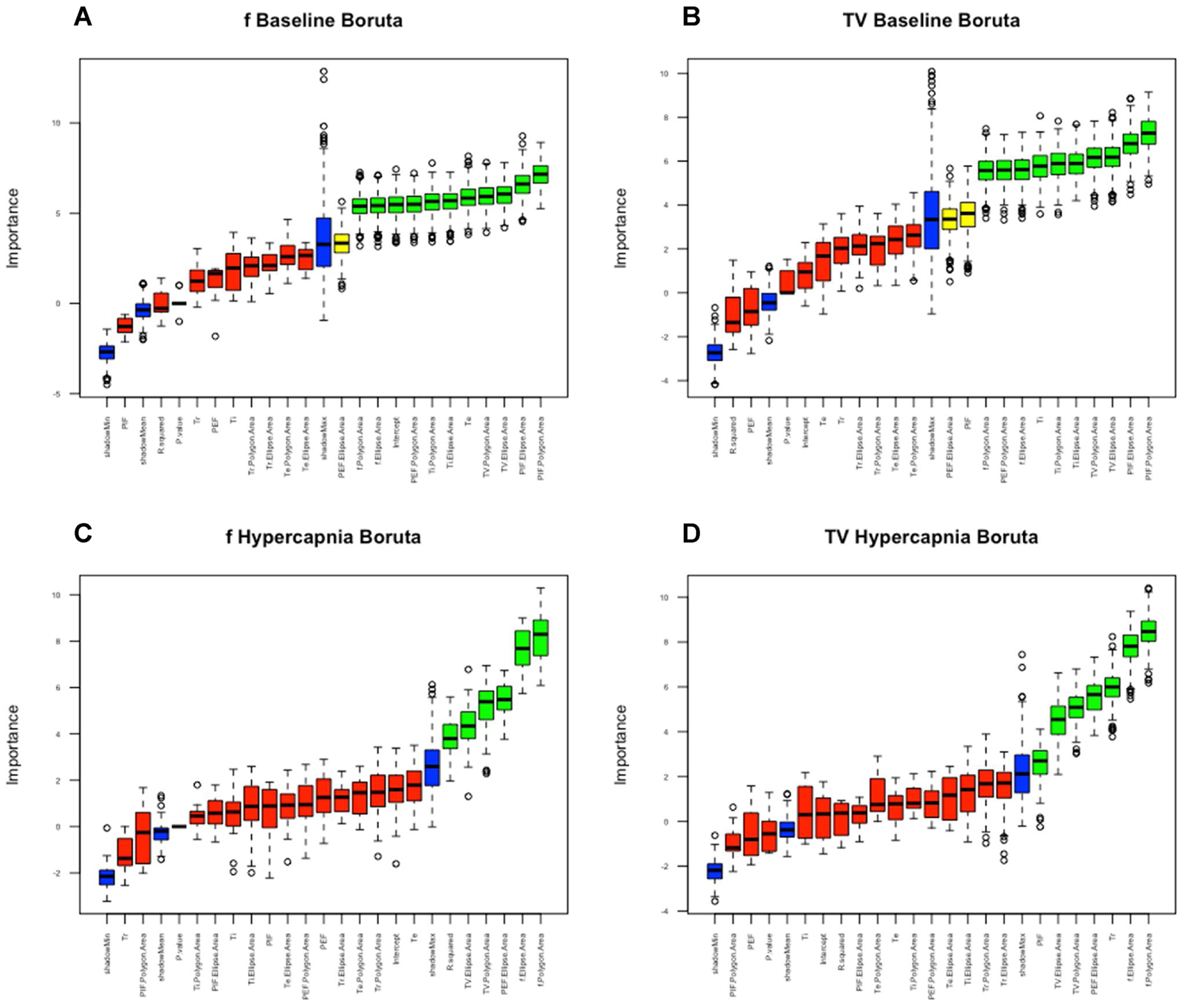
Boruta in R was utilized to identify which features were drivers for machine learning algorithms for models derived from f (A/C) and TV (B/D) and between baseline (A/B) and hypercapnic data (C/D). Features were compared against a shadow feature in blue that represents random reassortment of features. Red represents features which could not outperform their randomized counterpart. Green represents features which significantly outperformed their randomized features and yellow represents features which were indeterminate. Red features were removed in our decision models for machine learning algorithms.

3.6. Machine models with increased importance to parameter variation had highest performance

Utilizing the non-rejected features from the Boruta analysis, machine learning algorithms were trained with 60 % of the dataset in order to predict age on the remaining 40 % non-exposed test set. The selected machine learning algorithms were random forest, gradient boosted method and support vector machine. To measure performance of machine learning algorithms, developed machines were tested with confusion matrices to measure overall accuracy of predicted age labels against ground truth age labels (defined as accuracy). All models were trained independent of each other and were only challenged to predict age labels. Amongst the algorithms, support vector machines performed with accuracy scores of 91.67 %, 81.82 %, 87.5 % and 88.89 % within confusion matrices generated from baseline frequency models, baseline tidal volume models, hypercapnic frequency models and hypercapnic tidal volume models respectively. Random forest performed well with accuracy scores of 75 %, 90.91 %, 87.5 % and 100 %. Finally, gradient boosted method algorithms had confusion matrix accuracy scores of 66.67 %, 72.73 %, 87.5 % and 77.78 % (Fig. 15, A&B). To further analyze model performance, area under the curve (AUC) of receiver operating characteristics curves were calculated for each model to define the diagnostic ability of our classifiers. This was achieved by plotting the true positive rate against the false positive rate of each model’s predictions and calculating the area below the plotted line in R (with stronger diagnostic capability approaching 1). Support vector machines achieved AUCs of 0.833, 0.889, 0.9 and 0.9 for baseline frequency models, baseline tidal volume models, hypercapnic frequency models and hypercapnic tidal volume models respectively. Random forest models achieved AUCs of 0.875, 0.944, 0.9 and 1. Finally, gradient boosted machines had AUCs of 0.771, 0.833, 0.9 and 0.772 (Fig. 15, C&D). Algorithms were further evaluated based upon confusion matrix accuracy and AUC to identify key drivers that may have led to higher scores. Both support vector and random forest utilized a balanced mix of different parameter variations as strong drivers in predicting age. In contrast, gradient boosted heavily decided predictions by selecting a single specific feature to drive decision making (Fig. 15, E–H). This demonstrated that significant differences between the relationships of respiratory parameters could provide accurate prediction of mouse pup age. By interrogating the key drivers used by each learning algorithm, it was seen that respiratory variation of parameters was a strong driver of age differentiation.

Fig. 15. Machine learning accuracy is driven by equal distribution of features.

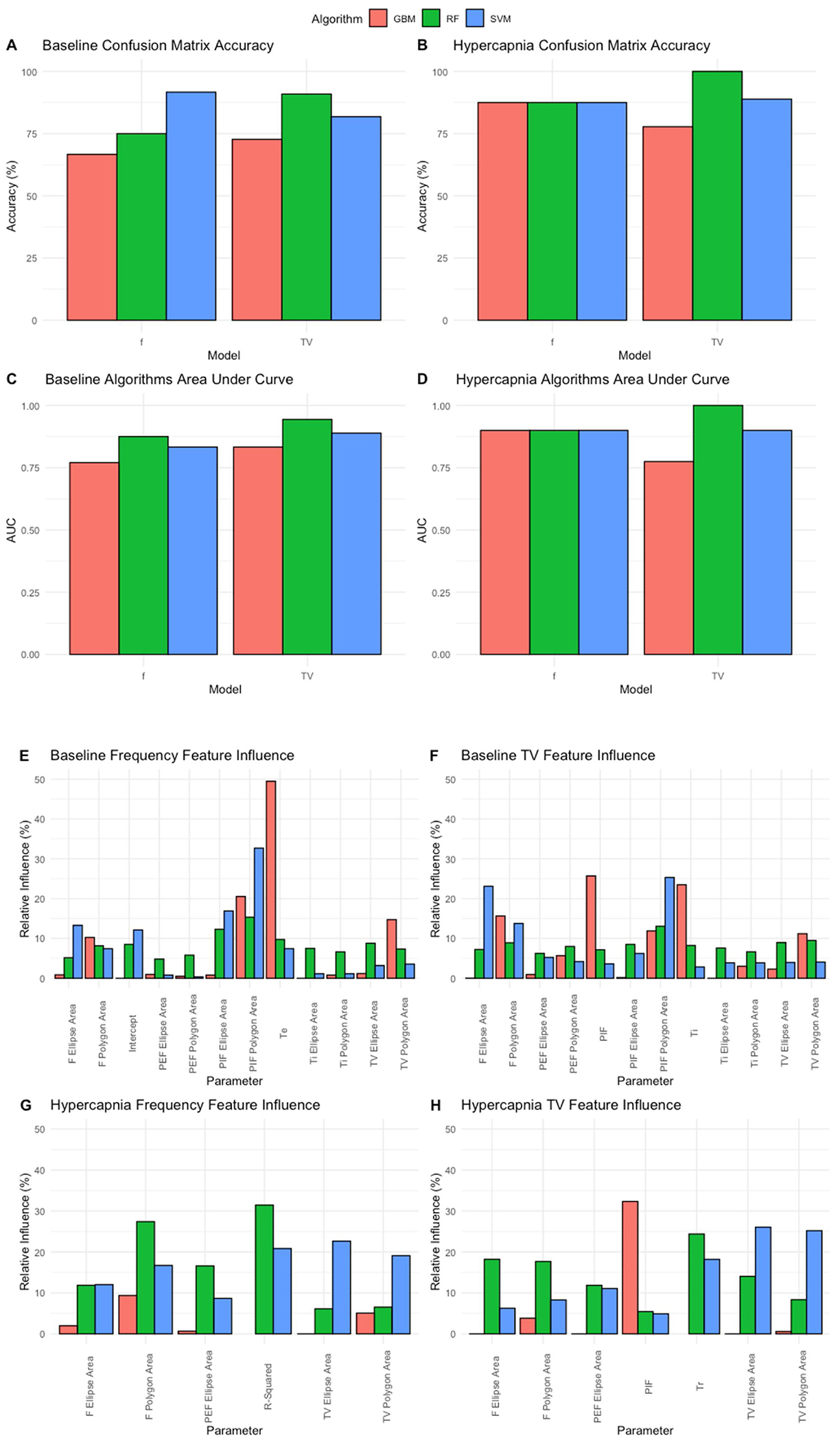
Machine learning algorithms were trained with 60 % of the data set and tested with the remaining 40 %. Accuracy was measured from confusion matrices for the following models gradient boosted method (red), random forest (green) and support vector (blue). Accuracies were compared among models and between frequency and tidal volume derived analysis from baseline (A) and hypercapnic breathing (B). Algorithms were further evaluated for classification ability utilizing area under the curve (AUC) values calculated within R for baseline (C) and hypercapnia models (D). Relative influence for model decisions were plotted for baseline frequency (E), baseline tidal volume (F), hypercapnic frequency (G) and hypercapnic tidal volume (H).

4. Discussion

Our understanding of the mechanisms by which neural circuits regulate breathing has been significantly aided by utilization of brainstem-spinal cord en bloc preparations, where the respiratory rhythm generator has been shown to maintain its bursting electrical activity for several hours ex vivo in fetal and newborn rodents (Di Pasquale et al., 1992; Greer et al., 1992; Hilaire et al., 1997; Viemari et al., 2003). The advent of commercially available plethysmograph systems has permitted the standardized evaluation of respiratory physiology in small rodents. Although a functional respiratory circuit is required for ex utero survival, several lines of evidence suggest that the respiratory system undergoes significant maturation. For instance, plethysmographic recordings of newborn pups (P3-P9, as well as E18 pup delivered by cesarean section) demonstrated significant changes in plethysmograph wave forms (Viemari et al., 2003). In these studies, single respiratory parameters (frequency, tidal volume, minute ventilation) were evaluated as a function of age and gas challenge, yet the relationships between respiratory parameters were not measured. Nevertheless, the findings of Viemari, et al. showed changes in variability of phrenic nerve bursts when comparing E16, P2, and P6 animals in accordance to the observations reported in our study.

It has been postulated that the serotonergic and catecholaminergic neurotransmitter systems are key contributors to this developmental maturation. For instance, pontine-derived projections, presumably through A5-dependent projections to the ventral lateral medulla, show different extents of inhibition in early preparations (~P0/1) relative to late preparations (~P3-P5) rats (Hilaire et al., 2004), and the number of A5 neurons in the rat pup reportedly decreases with advanced post-natal age (Ito et al., 2002). Biochemical evidence indicates that several neurotransmitters, including noradrenaline and serotonin, increase with advanced post-natal age at rates independent of total brain weight (Ide et al., 2005). Similarly, serotonergic neurons have been shown to play an essential role in the development and control of breathing (Hilaire et al., 2010). Serotonin has been shown to be critical for the formation of the premotor phrenic network (Bras et al., 2008), and perturbation of the serotonin system modulates the developing respiratory network (Zanella et al., 2008a, b). In summary, several evidences provided by previous pharmacologic, neurochemical, and physiological studies support the idea that the brainstem’s respiratory networks change as a function of post-natal age. However, appreciation of differences in ventilation at later post-natal ages has not been well appreciated due to the inherent noise of respiratory plethysmography systems. In our approaches, ML-based interpretation of these respiratory data was able to perceive differences between P21 and P56 animals, a feat not possible with conventional data analysis approaches.

To acknowledge however, in comparing respiratory parameters between a head-out plethysmography and whole body plethysmography approach, as respiratory activity has been shown to shift as a function of temperature, changes in pup body temperature during the duration of recording may underlie certain aspects of variability (Rubini and Bosco, 2013). In addition, while chambers were heated to lower the likelihood of this event, humidification, rarefaction and compression of the breathing environment is known to affect breathing parameters in similar experiments (Ray et al., 2011). Additionally, as P1 mice were restrained in the head out plethysmography configuration, potential stress may add to breathing variability in the group. However, the methodology was still successful in identifying difference in more mature P21 and P56 aged mice that underwent the same unrestrained whole-body plethysmography recording. Moreover, integration of chamber parameters to machine learning pipelines in future experiments may present methods by which to normalize for the differences in chamber environment as similar to the methods used to normalize for weight influence on breathing parameters in our manuscript.

In turn, while plethysmographic analyses show more noise in their data relative to en bloc or slice electrophysiological preparations, plethysmographic studies have the advantage that they represent a recording from an integrated system. Thus, the use of plethysmographic analyses permits the inclusion of multiple systemic parameters in study design but has the drawback that plethysmographic recordings represent large datasets with multiple variables extracted. Our data demonstrated that the key discriminating features of respiration that separate animals based on post-natal age are measures of respiratory variability, a finding in accordance with several other published reports (Patrone et al., 2018). The present data confirm the utility of machine-learning based workflows for the analysis of post-natal developmental maturation of the respiratory pattern. We posit that such approaches are time-efficient, less prone to bias compared to manual selection of plethysmograph tracings, and that interrogation of these models can generate novel hypotheses for investigators and should be adopted in developmental biology research.

5. Approaches to implement machine learning based workflows in developmental biology research

Developmental biology is now a so-called “big data” field. Although developmental biologists have embraced machine learning for large datasets such as microarray and RNAseq analyses, utilization of these similar approaches to other aspects of developmental biology has proceeded at a much slower pace. In the present workflow, we utilized a combination of supervised and unsupervised techniques to identify which respiratory parameters changed most significantly during postnatal development. Main component analysis, although often used as a dimensionality reduction tool in transcriptional assays, can be utilized to study the variance associated in any numerical dataset (Jolliffe and Cadima, 2016; Lu et al., 2011), and has been deployed in such diverse fields ranging from human clinical studies (Zhang and Castelló, 2017) to protein biophysics (David and Jacobs, 2014). In our workflow, we used PCA as a first step in analyzing the dataset to identify which features contributed most to the variance in the dataset. Using PCA for feature selection has been widely used in other bioinformatics pipelines (Hira and Gillies, 2015). We then utilized a linear discriminate analysis, a supervised dimensionality reduction technique that in some circumstances outperforms PCA in cluster separation (Lee et al., 2005). Using the LDA model, we found significant group separation could be observed. After that, we determined across all of the features the optimal cluster number by performing the gap statistic test for the kmeans cluster algorithm. Such analyses are used to study optimal cluster count by comparing change in within-cluster dispersion against a reference null distribution in an unsupervised manner (Tibshirani et al., 2001). By adding this step, we could objectively demonstrate that our data derives from three groups, thereby proving through distinct and independent tests that the three age groups can be distinguished based on these features.

A final step in our workflow included the construction of a class label prediction algorithm. Our work demonstrates that algorithmic reliable class label predictions can be made using respiratory metrics. These approaches also identify the most influential features to our analyses. The approaches used were modified for our purposes from other studies in the scientific literature (Degenhardt et al., 2019; Fortino et al., 2014; Kursa, 2014), which underscore the ease at which the machine learning “toolbox” can be implemented across disciplines and experimental paradigms. We show that mouse age could be identified using a spectrum of techniques (including support vector machines, random forest, and gradient boosted machines) that examining breathing metrics. These techniques allowed us to identify which features were most important in the classification. From these analyses, we can conclude that the polygon and ellipse areas of the tidal volume and the peak inspiratory flow derived from the Poincaré plots showed the highest importance in classification. As these features indicate changes in respiratory variability, we can conclude that this variability represents the most important feature that changes with age that was detected in our plethysmographic analyses.

Rapid phenotyping of transgenic mouse with developmental pathologies represents an area of high urgency by government funding agencies. For instance, in the United States, the National Institutes of Health has issued multiple rounds of mouse phenotyping pipeline program announcements (eg., PA-13–231, PA-7–005). Plethysmographic analysis was amongst the techniques advised by Solberg and colleagues advocating high throughput phenotyping of mouse phenotypes (Solberg et al., 2006). In summary, our study demonstrates the feasibility of incorporating machine learning tools into developmental biology phenotyping pipelines, which increase rigor and objectivity while decreasing the time needed for analysis and permitting evaluation of high dimensionality data across experimental measurements. Thus, integrating modern high throughput tools to assess physiological metrics such as breathing creates an avenue to effectively analyze data, generate novel hypotheses, and improve experimental rigor.

Fig. 8. Respiratory expiratory time (sec) variation shows changes with age and breathing state.

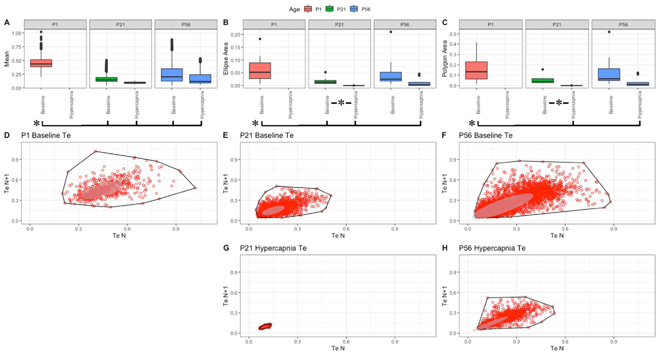
Parameter boxplots were generated to compare parameter mean (A), ellipse area (B) and polygon area (C) in P1, P21 and P56 in both baseline and hypercapnic states. P1 hypercapnia was omitted as previously mentioned in Fig. 1. Ellipse area was plotted as a confidence ellipse where center was the mean and the outer diameter contains 1 standard deviation of the dataset. Polygon areas were generated utilizing the extreme points which form the outer margin of each plot. Poincaré plots were generated from baseline breathing states (D–F) and hypercapnic states (G–H) to visualize variation in expiratoiy time (Te). T-tests were performed between age groups and breathing states for mean, polygon area and ellipse area. Bars and asterisks were utilized to represent significant variation between groups with p-values < 0.05.

Abbreviations:

f

frequency

TV

tidal volume

References

- Alheid GF, Milsom WK, McCrimmon DR, 2004. Pontine influences on breathing: an overview. Respiratory Physiology & Neurobiology. Pontine Influences in Breathing 143, 105–114. 10.1016/j.resp.2004.06.016. [DOI] [PubMed] [Google Scholar]
- Alzate-Correa D, Mei-Ling Liu J, Jones M, Silva TM, Alves MJ, Burke E, Zuñiga J, Kaya B, Zaza G, Aslan MT, Blackburn J, Shimada MY, Fernandes-Junior SA, Baer LA, Stanford KI, Kempton A, Smith S, Szujewski CC, Silbaugh A, Viemari J-C, Takakura AC, Garcia AJ, Moreira TS, Czeisler CM, Otero JJ, 2020. Neonatal apneic phenotype in a murine congenital central hypoventilation syndrome model is induced through non-cell autonomous developmental mechanisms. Brain Pathol. 10.1111/bpa.12877. [DOI] [PMC free article] [PubMed] [Google Scholar]
- Anderson TM, Garcia AJ, Baertsch NA, Pollak J, Bloom JC, Wei AD, Rai KG, Ramirez J-M, 2016. A novel excitatory network for the control of breathing. Nature 536, 76–80. 10.1038/nature18944. [DOI] [PMC free article] [PubMed] [Google Scholar]
- Bras H, Gaytán SP, Portalier P, Zanella S, Pásaro R, Coulon P, Hilaire G, 2008. Prenatal activation of 5-HT2A receptor induces expression of 5-HT1B receptor in phrenic motoneurons and alters the organization of their premotor network in newborn mice. Eur. J. Neurosci 28, 1097–1107. 10.1111/j.1460-9568.2008.06407.x. [DOI] [PubMed] [Google Scholar]
- Carroll JL, Kim I, 2005. Postnatal development of carotid body glomus cell O2 sensitivity. Respiratory Physiology & Neurobiology. Development of Respiratory Control 149, 201–215. 10.1016/j.resp.2005.04.009. [DOI] [PubMed] [Google Scholar]
- Chapin JL, 1954. Ventilatory response of the unrestrained and unanesthetized hamster to CO2. Am. J. Physiol 179, 146–148. 10.1152/ajplegacy.1954.179.1.146. [DOI] [PubMed] [Google Scholar]
- Czeisler CM, Silva TM, Fair SR, Liu J, Tupal S, Kaya B, Cowgill A, Mahajan S, Silva PE, Wang Y, Blissett AR, Göksel M, Borniger JC, Zhang N, Fernandes-Junior SA, Catacutan F, Alves MJ, Nelson RJ, Sundaresean V, Rekling J, Takakura AC, Moreira TS, Otero JJ, 2019. The role of PHOX2B-derived astrocytes in chemosensory control of breathing and sleep homeostasis. J. Physiol. (Lond.) 597, 2225–2251. 10.1113/JP277082. [DOI] [PMC free article] [PubMed] [Google Scholar]
- David CC, Jacobs DJ, 2014. Principal component analysis: a method for determining the essential dynamics of proteins. Methods Mol. Biol 1084, 193–226. 10.1007/978-1-62703-658-0_11. [DOI] [PMC free article] [PubMed] [Google Scholar]
- Degenhardt F, Seifert S, Szymczak S, 2019. Evaluation of variable selection methods for random forests and omics data sets. Brief. Bioinformatics 20, 492–503. 10.1093/bib/bbx124. [DOI] [PMC free article] [PubMed] [Google Scholar]
- Del Negro CA, Funk GD, Feldman JL, 2018. Breathing matters. Nat. Rev. Neurosci 19, 351–367. 10.1038/s41583-018-0003-6. [DOI] [PMC free article] [PubMed] [Google Scholar]
- Delgado-Bonal A, Marshak A, 2019. Approximate entropy and sample entropy: a comprehensive tutorial. Entropy 21, 541 10.3390/e21060541. [DOI] [PMC free article] [PubMed] [Google Scholar]
- Di Pasquale E, Monteau R, Hilaire G, 1992. In vitro study of central respiratory-like activity of the fetal rat. Exp. Brain Res 89, 459–464. 10.1007/BF00228263. [DOI] [PubMed] [Google Scholar]
- Dosumu-Johnson RT, Cocoran AE, Chang Y, Nattie E, Dymecki SM, 2018. Acute perturbation of Pet1-neuron activity in neonatal mice impairs cardiorespiratory homeostatic recovery. Elife 7 10.7554/eLife.37857. [DOI] [PMC free article] [PubMed] [Google Scholar]
- Drorbaugh JE, Fenn WO, 1955. A barometric method for measuring ventilation in newborn infants. Pediatrics 16, 81–87. [PubMed] [Google Scholar]
- Feldman JL, Del Negro CA, 2006. Looking for inspiration: new perspectives on respiratory rhythm. Nat. Rev. Neurosci 7, 232 10.1038/nrn1871. [DOI] [PMC free article] [PubMed] [Google Scholar]
- Flandre TD, Leroy PL, Desmecht DJ-M, 2003. Effect of somatic growth, strain, and sex on double-chamber plethysmographic respiratory function values in healthy mice. J. Appl. Physiol 94, 1129–1136. 10.1152/japplphysiol.00561.2002. [DOI] [PubMed] [Google Scholar]
- Fortino V, Kinaret P, Fyhrquist N, Alenius H, Greco D, 2014. A robust and accurate method for feature selection and prioritization from multi-class OMICs data. PLoS One 9, e107801 10.1371/journal.pone.0107801. [DOI] [PMC free article] [PubMed] [Google Scholar]
- Fox J, Weisberg S, 2011. An R Companion to Applied Regression. SAGE Publications. [Google Scholar]
- Gawlitza J, Sturm T, Spohrer K, Henzler T, Akin I, Schönberg S, Borggrefe M, Haubenreisser H, Trinkmann F, 2019. Predicting pulmonary function testing from quantified computed tomography using machine learning algorithms in patients with COPD. Diagnostics (Basel) 9 10.3390/diagnostics9010033. [DOI] [PMC free article] [PubMed] [Google Scholar]
- Gokozan HN, Baig F, Corcoran S, Catacutan FP, Gygli PE, Takakura AC, Moreira TS, Czeisler C, Otero JJ, 2016. Area postrema undergoes dynamic postnatal changes in mice and humans. J. Comp. Neurol 524, 1259–1269. 10.1002/cne.23903. [DOI] [PMC free article] [PubMed] [Google Scholar]
- Gray PA, 2013. Transcription factors define the neuroanatomical organization of the medullary reticular formation. Front. Neuroanat 7 10.3389/fnana.2013.00007. [DOI] [PMC free article] [PubMed] [Google Scholar]
- Greer JJ, Smith JC, Feldman JL, 1992. Respiratory and locomotor patterns generated in the fetal rat brain stem-spinal cord in vitro. J. Neurophysiol 67, 996–999. 10.1152/jn.1992.67.4.996. [DOI] [PubMed] [Google Scholar]
- Hawkins VE, Takakura AC, Trinh A, Malheiros-Lima MR, Cleary CM, Wenker IC, Dubreuil T, Rodriguez EM, Nelson MT, Moreira TS, Mulkey DK, 2017. Purinergic regulation of vascular tone in the retrotrapezoid nucleus is specialized to support the drive to breathe. Elife 6 10.7554/eLife.25232. [DOI] [PMC free article] [PubMed] [Google Scholar]
- Hilaire G, Bou C, Monteau R, 1997. Rostral ventrolateral medulla and respiratory rhythmogenesis in mice. Neurosci. Lett 224, 13–16. 10.1016/s0304-3940(97)13458-9. [DOI] [PubMed] [Google Scholar]
- Hilaire G, Viemari J-C, Coulon P, Simonneau M, Bévengut M, 2004. Modulation of the respiratory rhythm generator by the pontine noradrenergic A5 and A6 groups in rodents. Respir. Physiol. Neurobiol. 143, 187–197. 10.1016/j.resp.2004.04.016. [DOI] [PubMed] [Google Scholar]
- Hilaire G, Voituron N, Menuet C, Ichiyama RM, Subramanian HH, Dutschmann M, 2010. The role of serotonin in respiratory function and dysfunction. Respir. Physiol. Neurobiol 174, 76–88. 10.1016/j.resp.2010.08.017. [DOI] [PMC free article] [PubMed] [Google Scholar]
- Hira ZM, Gillies DF, 2015. A review of feature selection and feature extraction methods applied on microarray data. Adv. Bioinformatics 2015, 198363 10.1155/2015/198363. [DOI] [PMC free article] [PubMed] [Google Scholar]
- Ide S, Itoh M, Goto Y, 2005. Defect in normal developmental increase of the brain biogenic amine concentrations in the mecp2-null mouse. Neurosci. Lett 386, 14–17. 10.1016/j.neulet.2005.05.056. [DOI] [PubMed] [Google Scholar]
- Ito Y, Oyamada Y, Hakuno H, Yamaguchi K, 2002. Morphological analysis of developmental changes in pontine noradrenergic neuronal groups in the neonatal rat. Brain Res. 925, 107–109. 10.1016/s0006-8993(01)03256-5. [DOI] [PubMed] [Google Scholar]
- Jansen AH, Chernick V, 1983. Development of respiratory control. Physiol. Rev 63, 437–483. 10.1152/physrev.1983.63.2.437. [DOI] [PubMed] [Google Scholar]
- Jolliffe IT, Cadima J, 2016. Principal component analysis: a review and recent developments. Philosophical Transactions of the Royal Society A: Mathematical. Physical and Engineering Sciences 374, 20150202 10.1098/rsta.2015.0202. [DOI] [PMC free article] [PubMed] [Google Scholar]
- Kassambara A, Mundt F, 2020. factoextra: Extract and Visualize the Results of Multivariate Data Analyses. [Google Scholar]
- Kuhn M, 2008. Building predictive models in r using the caret package. J. Stat. Softw 28, 1–26. 10.18637/jss.v028.i05.27774042 [DOI] [Google Scholar]
- Kuhn M, Wing J, Weston S, Williams A, Keefer C, Engelhardt A, Cooper T, Mayer Z, Kenkel B, R Core Team, Benesty M, Lescarbeau R, Ziem A, Scrucca L, Tang Y, Candan C, Hunt T, 2020. caret: Classification and Regression Training. [Google Scholar]
- Kursa MB, 2014. Robustness of Random Forest-based gene selection methods. BMC Bioinformatics 15, 8 10.1186/1471-2105-15-8. [DOI] [PMC free article] [PubMed] [Google Scholar]
- Kursa MB, Rudnicki WR, 2010. Feature selection with the boruta package. J. Stat. Softw 36, 1–13. 10.18637/jss.v036.i11. [DOI] [Google Scholar]
- Lee J, Park KL, Song MH, Lee KJ, 2005. Arrhythmia classification with reduced features by linear discriminant analysis. In: 2005 IEEE Engineering in Medicine and Biology 27th Annual Conference. Presented at the 2005 IEEE Engineering in Medicine and Biology 27th Annual Conference, pp. 1142–1144. 10.1109/IEMBS.2005.1616623. [DOI] [PubMed] [Google Scholar]
- Liaw A, Wiener M, 2002. Classification and Regression by randomForest, 2, 5.. [Google Scholar]
- Lim R, Zavou MJ, Milton P-L, Chan ST, Tan JL, Dickinson H, Murphy SV, Jenkin G, Wallace EM, 2014. Measuring respiratory function in mice using unrestrained whole-body plethysmography. J. Vis. Exp 10.3791/51755. [DOI] [PMC free article] [PubMed] [Google Scholar]
- Lu J, Kerns RT, Peddada SD, Bushel PR, 2011. Principal component analysis-based filtering improves detection for Affymetrix gene expression arrays. Nucleic Acids Res. 39, e86 10.1093/nar/gkr241. [DOI] [PMC free article] [PubMed] [Google Scholar]
- Mei-Ling Liu J, Fair SR, Kaya B, Zuniga JN, Mostafa HR, Alves MJ, Stephens JA, Jones M, Aslan MT, Czeisler C, Otero JJ, 2018. Development of a novel FIJI-Based method to investigate neuronal circuitry in neonatal mice. Dev. Neurobiol 78, 1146–1167. 10.1002/dneu.22636. [DOI] [PMC free article] [PubMed] [Google Scholar]
- Mellen NM, Janczewski WA, Bocchiaro CM, Feldman JL, 2003. Opioid-induced quantal slowing reveals dual networks for respiratory rhythm generation. Neuron 37, 821–826. [DOI] [PMC free article] [PubMed] [Google Scholar]
- Meyer D, Dimitriadou E, Hornik K, Weingessel A, Leisch F, 2019. C++-code), C.-C. C. (libsvm, C++-code), C.-C.L (libsvm, 2019. e1071: Misc Functions of the Department of Statistics. Probability Theory Group (Formerly: E1071), TU Wien. [Google Scholar]
- Moreira TS, Takakura AC, Czeisler C, Otero JJ, 2016. Respiratory and autonomic dysfunction in congenital central hypoventilation syndrome. J. Neurophysiol 116, 742–752. 10.1152/jn.00026 [DOI] [PMC free article] [PubMed] [Google Scholar]
- Mortola JP, Frappell PB, 2013. Measurements of air ventilation in small vertebrates. Respir. Physiol. Neurobiol 186, 197–205. 10.1016/j.resp.2013.02.001. [DOI] [PubMed] [Google Scholar]
- Onodera M, Kuwaki T, Kumada M, Masuda Y, 1997. Determination of ventilatory volume in mice by whole body plethysmography. Jpn. J. Physiol 47, 317–326. 10.2170/jjphysiol.47.317. [DOI] [PubMed] [Google Scholar]
- Patrone LGA, Biancardi V, Marques DA, Bícego KC, Gargaglioni LH, 2018. Brainstem catecholaminergic neurones and breathing control during postnatal development in male and female rats. J. Physiol. (Lond.) 596, 3299–3325. 10.1113/JP275731. [DOI] [PMC free article] [PubMed] [Google Scholar]
- Pereira T, Ding C, Gadhoumi K, Tran N, Colorado RA, Meisel K, Hu X, 2019. Deep learning approaches for plethysmography signal quality assessment in the presence of atrial fibrillation. Physiol. Meas 40, 125002 10.1088/1361-6579/ab5b84. [DOI] [PMC free article] [PubMed] [Google Scholar]
- Ray R, Corcoran A, Brust R, Kim JC, Richerson GB, Nattie E, Dymecki SM, 2011. Impaired respiratory and body temperature control upon acute serotonergic neuron inhibition. Science 333, 637–642. 10.1126/science.1205295. [DOI] [PMC free article] [PubMed] [Google Scholar]
- Rose MF, Ahmad KA, Thaller C, Zoghbi HY, 2009a. Excitatory neurons of the proprioceptive, interoceptive, and arousal hindbrain networks share a developmental requirement for Math1. Proc. Natl. Acad. Sci. U.S.A 106, 22462–22467. 10.1073/pnas.0911579106. [DOI] [PMC free article] [PubMed] [Google Scholar]
- Rose MF, Ren J, Ahmad KA, Chao H-T, Klisch TJ, Flora A, Greer JJ, Zoghbi HY, 2009b. Math1 is essential for the development of hindbrain neurons critical for perinatal breathing. Neuron 64, 341–354. 10.1016/j.neuron.2009.10.023. [DOI] [PMC free article] [PubMed] [Google Scholar]
- Rubini A, Bosco G, 2013. The effect of body temperature on the dynamic respiratory system compliance–breathing frequency relationship in the rat. J. Biol. Phys 39, 411–418. 10.1007/s10867-013-9298-8. [DOI] [PMC free article] [PubMed] [Google Scholar]
- Smith JC, Ellenberger HH, Ballanyi K, Richter DW, Feldman JL, 1991. Pre-Bötzinger complex: a brainstem region that may generate respiratory rhythm in mammals. Science 254, 726–729. 10.1126/science.1683005. [DOI] [PMC free article] [PubMed] [Google Scholar]
- Sobrinho CR, Gocalves CM, Takakura AC, Mulkey DK, Moreira TS, 2017. Fluorocitrate-mediated depolarization of astrocytes in the retrotrapezoid nucleus stimulates breathing. J. Neurophysiol 118, 1690–1697. 10.1152/jn.00032.2017. [DOI] [PMC free article] [PubMed] [Google Scholar]
- Solberg LC, Valdar W, Gauguier D, Nunez G, Taylor A, Burnett S, Arboledas-Hita C, Hernandez-Pliego P, Davidson S, Burns P, Bhattacharya S, Hough T, Higgs D, Klenerman P, Cookson WO, Zhang Y, Deacon RM, Rawlins JNP, Mott R, Flint J, 2006. A protocol for high-throughput phenotyping, suitable for quantitative trait analysis in mice. Mamm. Genome 17, 129–146. 10.1007/s00335-005-0112-1. [DOI] [PubMed] [Google Scholar]
- Tibshirani R, Walther G, Hastie T, 2001. Estimating the number of clusters in a data set via the gap statistic. J. R. Stat. Soc. B 63, 411–423. 10.1111/1467-9868.00293. [DOI] [Google Scholar]
- Tupal S, Huang W-H, Picardo MCD, Ling G-Y, Del Negro CA, Zoghbi HY, Gray PA, 2014. Atoh1-dependent rhombic lip neurons are required for temporal delay between independent respiratory oscillators in embryonic mice. eLife 3 10.7554/eLife.02265. [DOI] [PMC free article] [PubMed] [Google Scholar]
- van der Heijden ME, Zoghbi HY, 2020. Development of the brainstem respiratory circuit. Wiley Interdiscip. Rev. Dev. Biol 9, e366 10.1002/wdev.366. [DOI] [PubMed] [Google Scholar]
- Vann NC, Pham FD, Dorst KE, Del Negro CA, 2018. Dbx1 pre-bötzinger complex interneurons comprise the core inspiratory oscillator for breathing in unanesthetized adult mice. eNeuro 5 10.1523/ENEURO.0130-18.2018. [DOI] [PMC free article] [PubMed] [Google Scholar]
- Venables WN, Ripley BD, 2002. Modern applied statistics with S Statistics and Computing, Statistics, Computing Venables, W.N.: Statistics w.S-PLUS, 4th ed. Springer-Verlag, New York, 10.1007/978-0-387-21706-2. [DOI] [Google Scholar]
- Viemari J-C, Burnet H, Bévengut M, Hilaire G, 2003. Perinatal maturation of the mouse respiratory rhythm-generator: in vivo and in vitro studies. Eur. J. Neurosci 17, 1233–1244. 10.1046/j.1460-9568.2003.02561.x. [DOI] [PubMed] [Google Scholar]
- Wang VY, Rose MF, Zoghbi HY, 2005. Math1 expression redefines the rhombic lip derivatives and reveals novel lineages within the brainstem and cerebellum. Neuron 48, 31–43. 10.1016/j.neuron.2005.08.024. [DOI] [PubMed] [Google Scholar]
- Wickham H, 2016. ggplot2: Elegant Graphics for Data Analysis, 2nd ed. Use R! Springer International Publishing; 10.1007/978-3-319-24277-4. [DOI] [Google Scholar]
- Yentes JM, Hunt N, Schmid KK, Kaipust JP, McGrath D, Stergiou N, 2013. The appropriate use of approximate entropy and sample entropy with short data sets. Ann. Biomed. Eng 41, 349–365. 10.1007/s10439-012-0668-3. [DOI] [PMC free article] [PubMed] [Google Scholar]
- Zanella S, Barthelemy M, Muscatelli F, Hilaire G, 2008a. Necdin gene, respiratory disturbances and Prader-Willi syndrome. Adv. Exp. Med. Biol 605, 159–164. 10.1007/978-0-387-73693-8_28. [DOI] [PubMed] [Google Scholar]
- Zanella S, Watrin F, Mebarek S, Marly F, Roussel M, Gire C, Diene G, Tauber M, Muscatelli F, Hilaire G, 2008b. Necdin plays a role in the serotonergic modulation of the mouse respiratory network: implication for Prader-Willi syndrome. J. Neurosci 28, 1745–1755. 10.1523/JNEUROSCI.4334-07.2008. [DOI] [PMC free article] [PubMed] [Google Scholar]
- Zhang Z, Castelló A, 2017. Principal components analysis in clinical studies. Ann. Transl. Med 5 10.21037/atm.2017.07.12. [DOI] [PMC free article] [PubMed] [Google Scholar]
Associated Data
This section collects any data citations, data availability statements, or supplementary materials included in this article.