Abstract
Background:
A Susceptible–Exposed–Infected–Removed (SEIR) model was developed to forecast the spread of the novel coronavirus (SARS-CoV-2) in the United States and the implications of re-opening and hospital resource utilization. The model relies on the specification of various parameters that characterize the virus and the population being modeled. However, several of these parameters can be expected to vary significantly between states. Therefore, a genetic algorithm was developed that adjusts these population-dependent parameters to fit the SEIR model to data for any given state.
Methods:
Publicly available data was collected from each state in terms of the number of positive COVID-19 cases and the number of COVID-19-caused deaths and used as inputs into a SEIR model to predict the spread of COVID infections in a given population. A genetic algorithm was designed where the genes are the state-dependent parameters from the model. The algorithm operates by determining the fitness of a given set of genes, applying selection, using selected agents to reproduce with cross-over, applying random mutation, and simulating several generations.
Findings and Conclusions:
Use of the genetic algorithm produces exceptionally good agreement between the model and available data. Deviations in the parameters were examined to see if the trends were reasonable.
Keywords: SARS-CoV-2, COVID-19, SEIR model, Genetic algorithm
1. Introduction
The COVID-19 pandemic in the US has been modeled for several states using a SEIR model adapted from Tang et al. [10], [11] with modifications. The SEIR model is described in greater detail by Yarsky in another paper [13] and in the interest of brevity the model is only summarized herein. In developing this model, there are several parameters that are state-dependent and will vary between states in the US. Reliable prediction of the course of the pandemic in any given state is predicated on determining reasonable values for the state-dependent parameters.
In the current work a genetic algorithm (see Mitchell et al. [7] and Qadrouh et al. [9]) is used to tune the state-dependent parameters such that the model produces good agreement with data for each state. The data in this case are the day-by-day tally of positive cases and the number of COVID-19 deaths, which are available fromwww.covidtracking.com [12]. An area of future work will be to study these parameter values in the light of other available data to determine if the suggested parameter values are reasonable and might be useful in forecasting.
2. Methods
The pandemic is modeled with a Susceptible–Exposed–Infected–Removed (SEIR) model. The basic elements are shown in Eqs. (1)–(5). The model tracks the evolution of different subpopulations, here S, E, I and R refer to the standard subpopulations and another population (A) is added to track asymptomatic individuals. In addition, a testing rate (shown in Eq. (6)) is modeled and the total number of positive cases is tracked according to Eq. (7). A novel element of the current work is to use the SEIR results to predict the rate at which diagnostic tests are performed and yield positive results (T’) and this testing rate is then used to compute a number of cases (C) for comparison to tabulated data on the number of cases in each state.
| (1) |
| (2) |
| (3) |
| (4) |
| (5) |
| (6) |
| (7) |
The model includes many parameters, some of which are virus-dependent (i.e., : pre-symptomatic transmission effectiveness 5%, : infection rate 0.2 days−1, : probability of developing symptoms 75%, : death rate 6.9 × 10⁻⁴ days−1, : recovery rate 0.14 days−1, : time between diagnostic test and result 3 days, and : diagnostic test false negative rate 5%). These parameter values were selected based on the available literature [13] and for additional detailed discussion the reader is referred to Yarsky [13]. However, some parameters will vary from state-to-state, most importantly the contact rate (c) but also, to a lesser extent, the transmission probability (), death rate (), the diagnostic test eligibility () and the test result period ().
Mitigation measures can be simulated in the SEIR model. Social distancing orders have the effect of reducing the contact rate (c). Mask wearing guidelines have the effect of reducing the transmission probability (). However, in addition to these effects from mitigation measures, there are differences in these parameters from state to state due to factors such as population density.
The contact rate will depend on the relative proportion of urban areas (where the routine contact rate is high) to rural areas in addition to impact of the social distancing measures in that state. The transmission probability may be sensitive to the weather [2], [6]. Furthermore, the death rate will be sensitivity to the number of people in the population with preexisting conditions that can increase the likelihood of a COVID-19 fatal outcome (e.g., diabetes) [8]. Finally, a state may have more easily assessable diagnostic testing and available lab capacity to process more tests compared to others. Therefore, the test eligibility and test result period may vary from state-to-state.
For a genetic algorithm to operate, several elements must be in place. For this discussion, the SEIR models a given state and predicts the cases (C) and deaths (D). It should be noted that the value of C gives the cumulative number of positive diagnostic test results for comparison to the tabulated data. The objective of the algorithm is to tune certain state-dependent parameters to achieve better agreement between the model and data. Each set of parameters for the SEIR model and the results of the run for that set will be referred to as an agent. Each agent has its input set of state-dependent parameters, which is the genome for that agent. For the genetic algorithm to tune these parameters, the agents must be judged based on their “fitness”, which measures how well the agent matches the available data.
Based on the fitness, some agents will be selected to reproduce and spawn new agents for the next generation. The new agents will have genomes that are subject to cross-over and random mutation based on the parent agent’s genome.
Successive generations are simulated until an agent produces results within an acceptable fitness threshold, or the total number of maximum generations are simulated.
Genetic algorithms have been used in various ways to improve modeling related to the novel coronavirus [1], [4]. The work of Ghosh et al. [4] is similar but that work appears to focus on case data as opposed to casualty data whereas the current work utilizes both case and casualty data in a novel fitness function. Carcione et al. [3] explain why SEIR model tuning should be performed using the casualty data because there are issues with using case and hospitalization data, and while Carcione was focused on modeling the pandemic in Italy, the observations are also applicable to the current work. The current work attempts to address some of the issues with using case data by including a case number equation and to improve the accuracy by utilizing the casualty data.
2.1. Genome
The genome is comprised by a list of the state-dependent parameters: normal contact rate, socially distant contact rate, transmission probability, death rate, test eligibility, mask wearing transmission reduction factor, and test period. Most of these are discussed in the introduction. The socially distant contact rate is the contact rate once a state has fully implemented all the available social distancing measures (e.g., school closures, business closures, stay-at-home order, etc.). The mask wearing transmission reduction factor characterizes the reduction in the transmission probability due to a significant portion of the population wearing face coverings in response to mask-wearing guidelines. It will vary from state-to-state depending on the proportion of people within that state that comply with the guidelines. Each parameter in the genome has an associated value which will be referred to as the gene. The value stored in the genome is the same value as used in the model. When a new genome is created from reproduction (i.e., a child’s genome), the child agent will run a SEIR model with parameters given by the genes in the child agent’s genome.
The genome includes the following genes in the following order: (1) normal contact rate, (2) socially distant contact rate (i.e., the contact rate when all social distancing measures are implemented), (3) the transmission probability, (4) the death rate, (5) test eligibility fraction, (6) the mask wearing transmission probability reduction factor, and (7) the test period.
2.2. Fitness
The fitness in the current work is calculated by taking the SEIR results and comparing to the available data in terms of cases and deaths. The fitness is a figure of merit that judges how well the SEIR model fits the available data. Since there are two data sets (cases and deaths) it is not appropriate to just use the root-mean-square difference as this would not necessarily properly take into account the vast difference in the number of cases compared to the number of deaths. Additionally, there might be large discrepancies in the data early in the outbreak due to two potential sources of bias: (1) cases predicted by the model are expected to be low because the SEIR model predicts cases based on diagnostic testing; however early in the outbreak cases were identified based on hospital diagnosis due to the presence of COVID-19 symptoms, so called presumptive cases, and (2) before testing confirmed the prevalence of COVID-19 many deaths may have been mischaracterized as non-COVID-19 deaths, meaning that the model will likely over-predict deaths early in the outbreak. Given these sources of bias, the fitness figure of merit was designed to more heavily weight the more recent data compared to the data from early in the outbreak.
The fitness is calculated according to Eq. (8). In this equation C(t) and D(t) are the cases and deaths at a given time (t). The subscripts d and m denote the data and the model result, respectively. The term T refers to the final day for which data is available.
| (8) |
The fitness function is similar to the root-mean-square (RMS) difference between the model and data in terms of cases and deaths. The differences are still squared, but are weighted with the ln(t), which slowly increases the importance of later data. The figures for cases and deaths are then divided by the total number of cases and deaths at the latest time (to normalize them). A factor of two is applied to the cases figure to increase the relative weight of the cases compared to the deaths. The normalization accounts for their being many more cases than deaths, but the factor of two restores some heavier weight to the cases-based figure.
One will notice that a model that produces very good agreement with the data will produce a low value for the fitness. This is an important note in the specific application of the genetic algorithm in this case. The selection element will select agents that have a low fitness score.
2.3. Selection
At the end of each generation, the agents in that generation are ranked according to their fitness. In the current work, a smaller fitness value means better agreement between the model and the data. A fixed percentage of the agents are selected for reproduction. In the current work, 20 percent are selected based on the suggestion of Mitchell et al. [7]. A genetic algorithm might weight the selection process using fitness, but instead just a list of the most fit agents were selected at a ratio of 20 percent which appears to yield enough diversity to allow exploration of the parameter space while still culling bad parameter sets. The current work uses 30 agents in each generation, so 6 agents are selected for reproduction after each generation. A number closer to 100 might give more robust performance of the algorithm, but a smaller number of agents reduces the computational expense, so there is a trade-off. Testing the algorithm indicated that 30 agents were sufficient to produce reliably good results.
2.4. Reproduction
The reproduction process selects two agents at random from the selected agents. These are selected randomly so there is the possibility for asexual reproduction (both parents happen to be the same agent). No special weight is given to higher fitness individuals once selection takes place; this preserves genetic diversity early in the process. Once two parent agents are selected, two children agents are produced. To create the child agents, child genomes are computed. For each pairing a cross-over factor is randomly selected, and the child genomes are calculated as follows in Eq. (9) where x is the cross-over factor and each gene in the genome is calculated in the same manner. Note, the cross-over is the same for every gene in genome for the pairing between two parents.
| (9.1) |
| (9.2) |
The next generation includes the selected agents from the previous generation, this ensures that the most fit agents continue to vie for selection in future generations, and then children are added through random pairings until the number of agents for the next generation is the same. In the current work, 30 agents are simulated in each generation, so the 6 selected agents from the previous generation are randomly paired to create 24 children for the subsequent generation.
2.5. Mutation
In addition to cross-over, after the children agents are spawned, there is a chance for random mutation. For all agents in the next generation — before any simulations are run, there is a fixed chance that a mutation will occur (in the current work 10 percent). A mutation rate that is too high hinders selection from increasing the allele frequency for favorable (i.e., more fit) genes; but a mutation rate that is too low stifles the genetic algorithm in that it will become more prone to finding localized optima rather than exploring a sufficient swath of parameter phase-space to garner a high likelihood for finding a truly optimum solution. Ten percent was selected in the current work as a decent balance between these competing effects. If a mutation occurs, a random agent is selected and a random gene within that agent’s genome is selected. That gene is then mutated by multiplying by a factor. The factor is randomly selected over a range from 0.75 to 1.25 in the current work. The mutation variability, much like the mutation rate should be selected to be large to ensure that the algorithm explores a wide variety of the parameter phase-space, but small enough that it does not preclude selection from favoring certain allele frequencies. The value of 25 percent was selected rather arbitrarily, but as shown in the results, the performance of the generic algorithm is acceptable with a manageable, tractable number of agents and generations.
2.6. Coarse-search acceleration
To accelerate the solution using the genetic algorithm, a “coarse-search” is done for the normal and socially distant contact rates upfront. These two values control the value of c during the simulation and are the most important because of their first order effect on the infection rate. It must be noted that the contact rate only appears in Eqs. (1), (2) as a product with the transmission probability. Therefore, as the contact rate is tuned, this compensates any error in the transmission probability because it is the product that affects the progression of the outbreak.
The coarse-search sweeps through a variety of discrete contact rate pairs. The discrete values are selected based on relatively large steps between a minimum and a maximum value; hence being called “coarse”. Several contact rate pairs are established and these are fed into SEIR models with all other genes set to default values. Runs are made for each pair and the fitness of each pair is used to sort the pairs into a “best-guess” pair. This is meant to establish a good initial guess for the contact rates before initializing the genetic algorithm search. Since the steps between the discrete pairs are relatively coarse this can be done at a small computational expense. Values between 1 and roughly 30–100 have been used here with a step size of 5 in the normal contact rate and a step size of 1 in the socially-distant contact rate.
2.7. Slicing and punctuated equilibria
The basic genetic algorithm operates over 50 generations, but is implemented to operate iteratively over sub-slices of the genome. In the first set of 50 generations, the algorithm operates only on three of the genes (normal contact rate, socially distant contact rate, and transmission probability). Fifty generations are run for this first slice. After completing those 50 generations, the slice is increased so the number of genes in the genome increases to include one more gene (the virus death rate). The process repeats and each slice includes one additional gene until every single gene is in the genome for the final run of the genetic algorithm. Each slice is subject to the genetic algorithm for 50 generations. This iterative approach with genome slicing simulates a kind of punctuated equilibrium [5] in the optimization process.
After each slice goes through the genetic algorithm, the most fit agent starts the next slice with one additional gene. But, to populate the first generation, agents are created by taking the initial agent and spawning 29 additional agents where every single gene is forced to randomly mutate. This has the effect of creating a new species after each slice is analyzed (by adding another gene to the genome) and then the genetic diversity is forced to increase at the start of the process for each slice. This can lead to a burst in the change in fitness for each slice — which is very much like punctuated equilibrium.
3. Results and discussion
The genetic algorithm was used to fit the SEIR model to five American states (Georgia, Michigan, New York, Pennsylvania, and Virginia). The genetic algorithm results are provided in Table 1. In the predecessor work (see Yarsky [13]), the SEIR model tends to under-predict the number of cases and over-predict the number of casualties early in the outbreak, this tendency was attributed to potential biases in the data themselves and the model can be expected to be biased in this manner. Briefly, the model only considers cases that are identified from a diagnostic test, but state-by-state case data include cases that were identified without such testing, especially early in the outbreak. However, when compared to the results produced with the genetic algorithm, the agreement between the model and data is greatly improved at later times even though similar biases are observed in the earliest phase of the outbreak.
Table 1.
Genetic algorithm results.
| DC | GA | MI | NY | PA | VA | |
|---|---|---|---|---|---|---|
| c initial [day −1] | 1.1E−06 | 8.6E−08 | 2.3E−07 | 9.1E−08 | 1.2E−07 | 1.1E−07 |
| c social distancing [day −1] | 5.3E−07 | 1.5E−08 | 1.8E−08 | 1.5E−08 | 2.3E−08 | 5.4E−08 |
| c social distancing + mask wearing [day −1] | 1.6E−07 | 4.8E−09 | 5.9E−09 | 5.2E−09 | 7.1E−09 | 1.6E−08 |
| [day −1] | 1.3E−03 | 7.7E−04 | 1.2E−03 | 8.6E−04 | 8.4E−04 | 9.9E−04 |
| 18% | 13% | 10% | 10% | 11% | 20% | |
| [days] | 3 | 3 | 3 | 3 | 3 | 3 |
| Cases relative RMS difference | 2.5% | 4.0% | 5.1% | 3.0% | 2.6% | 1.7% |
| Deaths relative RMS difference | 4.0% | 2.5% | 9.9% | 2.9% | 9.8% | 1.8% |
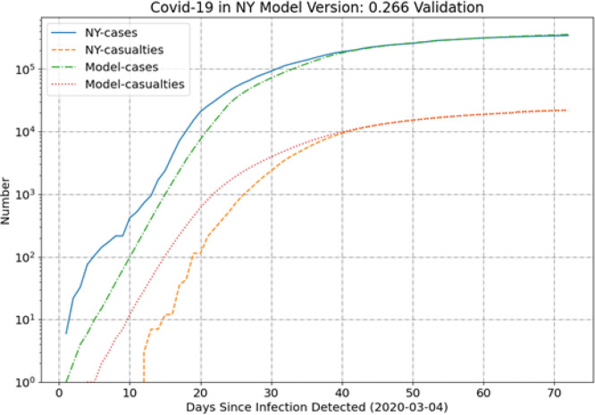
New York (NY) has the largest outbreak in the US at the drafting of this paper and Fig. 1 illustrates the model comparison to the data for this state. To compare the data and the SEIR results on a consistent basis the -axis reflects the number of days since the infection is detected, day 1 is thus labeled as the day when the number of cases (C) increases from 0 to 1. This state illustrates the general trend of under-predicting cases and over-predicting casualties during the first month. The model and data come into excellent agreement over the most recent 30 days. This is expected, however, since the fitness function more heavily weights the more recent data by design.
Fig. 1.
NY results.
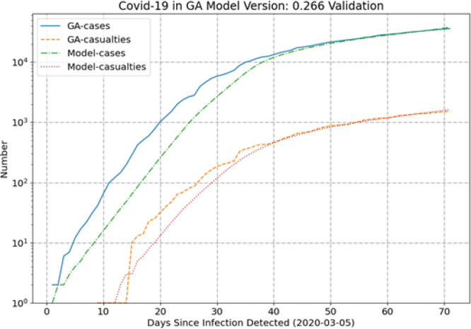
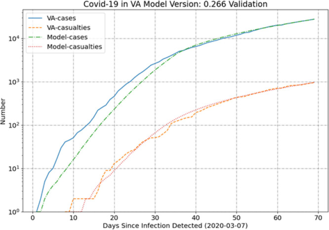
Georgia (GA) is notable in that the model tends to under-predict the casualties early, as shown in Fig. 2. Much like NY, however, the model and data come into very good agreement for the most recent 30 days. Virginia (VA) also deviates from the trend in the casualties, but instead of a clear bias the casualties are well predicted over the whole simulation period (see Fig. 3).
Fig. 2.
GA results.
Fig. 3.
VA results.
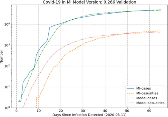
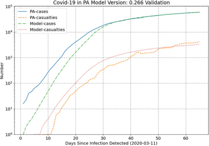
Results are also provided for Michigan (MI) and Pennsylvania (PA) in Fig. 4 and Fig. 5, respectively. The MI results are interesting in that this represents the current case with the poorest agreement between model and data. As can be seen in Table 1, the relative root-mean-square (RMS) differences between cases and casualties are highest for MI and then somewhat smaller for PA. These two states show larger deviations than the balance of states analyzed as part of the current work.
Fig. 4.
MI results.
Fig. 5.
PA results.
The MI data are an outlier compared to the data for the other states because of the unusual shift in the case trend around 15 days. There is a sharp change in the slope of the case trend and the SEIR model does not capture this rapid change in the trend well. As a result, it appears that the model will begin to start significantly under-predicting cases and casualties in the future. An area of future work would be to change the fitness function to even more heavily weight the more recent data, by perhaps using a (ln(t)) [11] weighting or something similar. This would likely improve the long-term predictive efficacy of the MI SEIR model at the expense of creating greater divergence in the earlier results.
The PA results in Fig. 5 show better agreement between model and data than MI, but the results for the casualties are interesting. It appears that the model can capture the trend of the casualties with the longer-term slope of the curve being in excellent agreement, but the SEIR model under-predicts the data by an approximately constant factor in the most recent two weeks. The PA data do include some quirks that may introduce deviations from expected values. Most significantly, there is a decrease in the deaths between 40 and 50 days. It is not clear why the data show this decrease, perhaps it was a recategorization of COVID-19 deaths as non-COVID-19 deaths, but it is not clear. Some irregularities like this in the data may explain the larger variation in the PA casualty data around the average trend (which is in good agreement with the model result).
While this initial study using the genetic algorithm indicates promise that the SEIR model predictions can be improved, there remains more work that must be done to verify the performance of the algorithm. A multitude of parameter combinations may provide results that seem reasonable when comparing to the data in an integral sense, but the individual parameters may be unreasonable. Therefore there is the potential for the proposed technique to produce results that may yield unrealistic predictions. As an area of future work, one might simulate multiple agents to determine a range of different parameter values that produce acceptable results when compared to the data. These parameter ranges must be compared from state-to-state to ensure that deviations are reasonable when considered with other data. As an example, cell phone mobility data may be useful in establishing if differences in contact rate are reasonable. Similar surrogate data could be used for the other parameters as well. Another avenue for independent model validation would be to examine the subpopulation results (i.e., the E and I results) and compare the model predictions with serological survey data to see if the model results are reasonable if such data exists for a given state.
The current work has focused on comparison of the SEIR model to data from early in the pandemic and an area of future work would be to expand the comparisons using data from later in 2020. However, the calculation of the number of cases currently includes an inherent assumption that diagnostic testing is rationed based on symptom severity. Many states have taken steps during 2020 to greatly expand their citizens’ access to diagnostic testing, which would limit the applicability of the current model to accurately calculate the number of cases later in the pandemic. Therefore, future work must also address the testing accessibility before the genetic algorithm can be used to adjust model parameters for data from much later in the pandemic.
4. Conclusions
The current work has demonstrated the use of a genetic algorithm to fit SEIR models of US states to available data. The current results are promising even though there are some cases (e.g., MI) where the comparison is not favorable, but some more investigation of the underlying data or refinements to the fitness function may improve the results. One potential avenue for improvement is to include hospitalization data in the fitness function to supplement the case and casualty data. In general, the SEIR model tends to under-predict cases and over-predict deaths early in the outbreak, but these biases can be expected based on assumptions in the model and biases in the underlying data sets. The fitness function proposed and utilized in the current work includes a weighting to focus the selection on more recent data. The results over many states indicate consistent good agreement between the model and data using the current implementation. However, the results require further scrutiny before they can be used for reliable predictions. An area of future work is to study state-by-state variations in the parameters and determine if these variations are reasonable based on surrogate data, such as mobility data in the case of the contact rate.
The current genetic algorithm utilizes two enhancements to improve the calculation performance: (1) an acceleration technique that uses a coarse-search of the contact rate to start the genetic algorithm with a better initial guess of the contact rates, and (2) a slicing method of the genome to evolve the model parameters in stages — the slicing method allows the genetic algorithm to spawn new species and thereby mimic punctuated equilibria during the process, which can lead to bursts of improvement in the fitness.
Declaration of Competing Interest
The authors declare that they have no known competing financial interests or personal relationships that could have appeared to influence the work reported in this paper.
References
- 1.Ardabili . 2020. COVID-19 outbreak prediction with machine learning. https://www.medrxiv.org/content/10.1101/2020.04.17.20070094v1. (Accessed 20 October 2020) [Google Scholar]
- 2.Bukhari Qasim, Jameel Yusuf. 2020. Will coronavirus pandemic diminish by summer? Available at SSRN 3556998. [Google Scholar]
- 3.Carcione J.M., Santos J.E., Bagaini C., Ba J. A simulation of a COVID-19 epidemic based on a deterministic SEIR model. Front. Public Health. 2020;8:230. doi: 10.3389/fpubh.2020.00230. [DOI] [PMC free article] [PubMed] [Google Scholar]
- 4.Ghosh S., Bhattacharya S. A data-driven understanding of COVID-19 dynamics using sequential genetic algorithm based probabilistic cellular automata. Appl. Soft Comput. J. 2020;96:1–12. doi: 10.1016/j.asoc.2020.106692. [DOI] [PMC free article] [PubMed] [Google Scholar]
- 5.Gould Stephen Jay, Eldredge Niles. Punctuated equilibria: an alternative to phyletic gradualism. Essent. Read. Evol. Biol. 1972:82–115. [Google Scholar]
- 6.Lipsitch M. 2020. Will COVID-19 go away on its own in warmer weather? Center for Communicable Disease Dynamics (CCDD) at the Harvard T.H. Chan School of Public Health. https://ccdd.hsph.harvard.edu/will-covid-19-go-away-on-its-own-in-warmer-weather/. (Accessed 5 March 2020) [Google Scholar]
- 7.Melanie Mitchell, James P. Crutchfield, Rajarshi Das, Evolving cellular automata with genetic algorithms: A review of recent work, in: Proceedings of the First International Conference on Evolutionary Computation and its Applications, EvCA’96, Vol. 8, 1996.
- 8.Preliminary estimates of the prevalence of selected underlying health conditions among patients with coronavirus disease 2019 — United States, February 12–March 28, 2020. MMWR Morb. Mortal. Wkly. Rep. 2020;69:382–386. doi: 10.15585/mmwr.mm6913e2. [DOI] [PMC free article] [PubMed] [Google Scholar]
- 9.Qadrouh A.N., Carcione J.M., Alajmi M., Alyousif J. A tutorial on machine learning with geophysical applications. Boll. Geofis. Teor. Appl. 2019;60(3):375–402. [Google Scholar]
- 10.Tang Biao, Bragazzi Nicola Luigi, Li Qian, Tang Sanyi, Xiao Yanni, Wu Jianhong. An updated estimation of the risk of transmission of the novel coronavirus (2019-nCov) Infect. Dis. Modell. 2019;5:248–255. doi: 10.1016/j.idm.2020.02.001. [DOI] [PMC free article] [PubMed] [Google Scholar]
- 11.Tang Biao, Wang Xia, Li Qian, Bragazzi Nicola Luigi, Tang Sanyi, Xiao Yanni, Wu Jianhong. Estimation of the transmission risk of the 2019-nCoV and its implication for public health interventions. J. Clin. Med. 2019;9(2):462. doi: 10.3390/jcm9020462. [DOI] [PMC free article] [PubMed] [Google Scholar]
- 12.2020. The COVID Tracking Project. www.covidtracking.com. (Accessed 15 May 2020) [Google Scholar]
- 13.Yarsky P. A simple COVID-19 model applied to American states to simulate mitigation and containment strategies. J. Glob. Health Rep. 2020;4 [Google Scholar]


